Affine Invisibility and Weak Identification in Correlation-Based Transformation Selection

1. Introduction

Parametric transformations are widely used to reduce skewness, stabilize variance, improve approximate normality, or linearize relationships between variables. Classical examples include logarithmic and power transformations, the Box–Cox family, and related transformation classes [1,2,3]. In exploratory analysis and model building, transformation parameters may also be selected by maximizing Pearson correlation, the coefficient of determination, or another criterion based on linear association [4,5]. A direct example is the Box–Cox linearity plot, which selects the transformation parameter by maximizing the correlation between a response and a transformed predictor [6]. Correlation maximization also underlies probability-plot correlation coefficient methods [7]; in a Box–Cox flood-frequency application, Lye [8] proposed selecting $\lambda$ by maximizing the corresponding probability-plot correlation. This paper studies the identification properties of such correlation-based selection. The question is not whether correlation maximization should replace likelihood-based estimation when a well-specified likelihood is available. Rather, we ask how informative Pearson correlation is as a functional for distinguishing among transformation parameters. Distinct parameter values may produce nearly identical correlation values, so a maximizing parameter need not be strongly identified by the criterion.

The mechanism is geometric and follows from the local invariance of Pearson correlation under additive shifts and positive rescalings. Let

$$U_{\theta }=T_{\theta }\left(X\right),V_{\eta }=S_{\eta }\left(Y\right),$$

and consider a parameter-space direction inducing the functional tangent ${\dot{T}}_{\theta ,a}\left(X\right)$. If

$${\dot{T}}_{\theta ,a}\left(X\right)={\alpha }_a+{\beta }_a{U}_{\theta }+R_a,R_a\perp span\{1,U_{\theta }\},$$

then the affine component is locally invisible to Pearson correlation and the directional derivative depends only on the residual component:

$$D_a\rho (\theta ,\eta )={\displaystyle \frac{Cov(R_a,V_{\eta })}{{\sigma }_{U_{\theta }}{\sigma }_{V_{\eta }}}}.$$

We refer to this property as affine invisibility. It provides a direct mechanism for weak local discrimination: if admissible perturbations are nearly affine in the current transformed scale, or if their non-affine residuals have little alignment with the other transformed variable, the correlation criterion has little first-order ability to discriminate among nearby parameter values. When such low visibility persists over a nontrivial parameter region, it can contribute to weak identification in the criterion-specific sense developed below.

The general result is then examined through log-polynomial directions. Their role is motivated by the Box–Cox family, whose expansion around the logarithmic case is

$${\displaystyle \frac{x^{\lambda }-1}{\lambda }}=logx+{\displaystyle \frac{\lambda }{2}}{(logx)}^2+{\displaystyle \frac{{\lambda }^2}{6}}{(logx)}^3+{\displaystyle \frac{{\lambda }^3}{24}}{(logx)}^4+\dots .$$

Thus, the Box–Cox path generates successive powers of $logx$ as its natural local functional directions. This representation allows the general geometric result to be studied componentwise and along the full Box–Cox path, without treating the Box–Cox family as an isolated special case.

The paper makes three contributions. First, it derives the directional sensitivity of Pearson correlation for general smooth transformation paths. Second, it identifies the non-affine residual of the induced functional tangent as the only component contributing to first-order correlation sensitivity. Third, it develops complementary local-visibility and near-optimality diagnostics, illustrating the former for log-polynomial directions and along the Box–Cox path, where scale-free visibility is maximal at the logarithmic case $\lambda =0$ and decreases as $\left|\lambda \right|$ increases over the range considered. Together, these diagnostics distinguish local insensitivity from global flatness of the correlation objective and provide a practical way to assess whether a correlation-selected transformation parameter is strongly or weakly identified.

The remainder of the paper develops the general correlation-based framework, derives the affine-invisibility result, discusses its implications for weak identification, specializes the analysis to log-polynomial and Box–Cox transformations, and presents analytical illustrations.

2. Correlation-Based Transformation Selection

Let X and Y be real-valued random variables defined on a common probability space $(\Omega ,\mathcal{F},P)$, and let

$$U_{\theta }=T_{\theta }\left(X\right),V_{\eta }=S_{\eta }\left(Y\right),$$

where $\theta \in \Theta \subseteq {\mathbb{R}}^p$ and $\eta \in \mathcal{E}\subseteq {\mathbb{R}}^q$. Throughout the paper, transformed variables and functional perturbations are regarded as elements of the common Hilbert space $L^2\left(P\right)$. Functions depending only on X or only on Y may be identified with the corresponding closed subspaces of $L^2\left(P\right)$. The inner product is

$${\langle A,B\rangle }_{L^2\left(P\right)}=\mathbb{E}\left(AB\right).$$

For centered elements, the $L^2$ inner product coincides with covariance. Orthogonality and projection are understood with respect to this $L^2$ geometry. We assume that the transformed variables have finite, non-zero variances over the parameter region under study. A correlation-based transformation rule selects parameters by maximizing

$$(\widehat{\theta },\widehat{\eta })\in arg\underset{\theta \in \Theta ,\eta \in \mathcal{E}}{max}{\rho }^2(\theta ,\eta ),$$

(1)

where

$$\rho (\theta ,\eta )=Corr\{T_{\theta }\left(X\right),S_{\eta }\left(Y\right)\}.$$

(2)

Empirically, $\rho$ is replaced by sample correlation and the criterion is evaluated over a parameter grid or by numerical optimization.

The criterion is attractive when transformations are chosen to improve a linear representation of dependence [2,5], but it uses only a standardized measure of linear association. It is therefore not equivalent to likelihood-based estimation and need not identify transformation parameters sharply. A high maximizing correlation may coexist with many alternative parameter values producing nearly the same objective value.

For $\epsilon >0$, define the near-optimal set

$${\mathcal{N}}_{\epsilon }=\left\{(\theta ,\eta )\in \Theta \times \mathcal{E}:{\rho }_{max}^2-{\rho }^2(\theta ,\eta )\le \epsilon \right\},$$

(3)

with

$${\rho }_{max}^2=\underset{\theta \in \Theta ,\eta \in \mathcal{E}}{sup}{\rho }^2(\theta ,\eta ).$$

A broad or elongated ${\mathcal{N}}_{\epsilon }$ indicates that the criterion provides weak discrimination among competing transformation parameters. Accordingly, we use the following criterion-specific notion.

Definition 1

(Weak identification under correlation-based selection). A transformation parameter is weakly identified by the correlation criterion when substantially different parameter values yield nearly indistinguishable values of ${\rho }^2(\theta ,\eta )$, producing broad near-optimal regions of the objective surface.

This notion concerns identification by the correlation criterion itself, not intrinsic identification in a fully specified statistical model. It is therefore distinct from the formal weak-identification asymptotics developed, for example, for instrumental-variable and generalized-method-of-moments settings [9,10]. Here the term refers specifically to weak discrimination among transformation parameters by the correlation objective. The next section shows that such weak discrimination has a simple local geometric source: Pearson correlation is insensitive to the affine component of an induced functional perturbation, so only its non-affine residual can affect the criterion to first order.

3. Affine Invisibility of Pearson Correlation

Let

$$U_{\theta }=T_{\theta }\left(X\right),V_{\eta }=S_{\eta }\left(Y\right),\rho (\theta ,\eta )=Corr(U_{\theta },V_{\eta }),$$

and consider a perturbation of $T_{\theta }$, with $S_{\eta }$ fixed. For a parameter-space direction $a\in {\mathbb{R}}^p$, define the induced functional tangent

$${\dot{T}}_{\theta ,a}\left(X\right)={\left.{\displaystyle \frac{d}{dt}}{T}_{\theta +ta}\left(X\right)\right|}_{t=0},$$

assuming existence in $L^2\left(P\right)$.

Project this tangent onto the subspace generated by the constant function and the current transformed variable. Thus,

$${\dot{T}}_{\theta ,a}\left(X\right)={\alpha }_{\theta ,a}+{\beta }_{\theta ,a}{U}_{\theta }+R_{\theta ,a}\left(X\right),$$

(4)

where

$$\mathbb{E}\left\{R_{\theta ,a}\left(X\right)\right\}=0,Cov\{R_{\theta ,a}\left(X\right),U_{\theta }\}=0.$$

The first two terms form the affine component of the perturbation; the residual $R_{\theta ,a}$ is its component orthogonal to $span\{1,U_{\theta }\}$.

It is useful to make explicit the functional-analytic structure behind this decomposition. For fixed $V_{\eta }$, define the Pearson-correlation functional

$${\mathcal{R}}_{V_{\eta }}\left(U\right)=Corr(U,V_{\eta }),$$

on the subset of $L^2\left(P\right)$ consisting of non-degenerate U. This functional is not linear, because its normalization depends on ${\sigma }_U$. However, at a fixed $U_{\theta }$, its derivative is a linear functional of the perturbation direction $H\in L^2\left(P\right)$, defined by

$$D{\mathcal{R}}_{V_{\eta }}\left(U_{\theta }\right)\left[H\right]={\left.{\displaystyle \frac{d}{dt}}Corr(U_{\theta }+tH,V_{\eta })\right|}_{t=0}.$$

A direct calculation gives

$$D{\mathcal{R}}_{V_{\eta }}\left(U_{\theta }\right)\left[H\right]={\displaystyle \frac{Cov(H,V_{\eta })}{{\sigma }_{U_{\theta }}{\sigma }_{V_{\eta }}}}-\rho (\theta ,\eta ){\displaystyle \frac{Cov(H,U_{\theta })}{{\sigma }_{U_{\theta }}^2}}.$$

(5)

Thus the directional derivative induced by the parameter-space direction a can be written as the composition

$$D_a\rho (\theta ,\eta )=D{\mathcal{R}}_{V_{\eta }}\left(U_{\theta }\right)\left[{\dot{T}}_{\theta ,a}\left(X\right)\right].$$

Moreover, every affine perturbation $H=\alpha +\beta U_{\theta }$ belongs to the kernel of this derivative:

$$D{\mathcal{R}}_{V_{\eta }}\left(U_{\theta }\right)\left[H\right]=0.$$

Equivalently,

$$span\{1,U_{\theta }\}\subseteq kerD{\mathcal{R}}_{V_{\eta }}\left(U_{\theta }\right).$$

The proposition below expresses the same fact through the orthogonal residual of the induced functional tangent.

Proposition 1

(Affine invisibility of Pearson correlation). Assume that $U_{\theta }$ and $V_{\eta }$ have finite, non-zero variances and that differentiation under the expectation sign is justified. Then

$$D_a\rho (\theta ,\eta )={\displaystyle \frac{Cov\{R_{\theta ,a}\left(X\right),V_{\eta }\}}{{\sigma }_{U_{\theta }}{\sigma }_{V_{\eta }}}},$$

(6)

where ${\sigma }_{U_{\theta }}^2=Var\left(U_{\theta }\right)$ and ${\sigma }_{V_{\eta }}^2=Var\left(V_{\eta }\right)$. Consequently,

$$D_a{\rho }^2(\theta ,\eta )=2\rho (\theta ,\eta ){\displaystyle \frac{Cov\{R_{\theta ,a}\left(X\right),V_{\eta }\}}{{\sigma }_{U_{\theta }}{\sigma }_{V_{\eta }}}}.$$

(7)

Proof. 

Write $U=U_{\theta }$, $V=V_{\eta }$, and $\dot{U}={\dot{T}}_{\theta ,a}\left(X\right)$. Differentiation of $\rho =Cov(U,V)/\left({\sigma }_U{\sigma }_V\right)$ with respect to the perturbation of U gives

$$D_a\rho ={\displaystyle \frac{Cov(\dot{U},V)}{{\sigma }_U{\sigma }_V}}-\rho {\displaystyle \frac{Cov(\dot{U},U)}{{\sigma }_U^2}}.$$

Using (4) and the orthogonality of $R_{\theta ,a}$,

$$Cov(\dot{U},V)={\beta }_{\theta ,a}Cov(U,V)+Cov(R_{\theta ,a},V),Cov(\dot{U},U)={\beta }_{\theta ,a}{\sigma }_U^2.$$

The terms involving ${\beta }_{\theta ,a}$ cancel, yielding (6); the expression for ${\rho }^2$ follows from the chain rule. □

Equation (6) is the key structural result: the affine part of an induced perturbation is locally invisible to Pearson correlation. In particular, if ${\dot{T}}_{\theta ,a}\left(X\right)={\alpha }_{\theta ,a}+{\beta }_{\theta ,a}{U}_{\theta }$, then $R_{\theta ,a}=0$ and hence $D_a\rho (\theta ,\eta )=0$.

The same argument applies when the second transformation is perturbed. If $b\in {\mathbb{R}}^q$ and

$${\dot{S}}_{\eta ,b}\left(Y\right)={\gamma }_{\eta ,b}+{\delta }_{\eta ,b}{V}_{\eta }+Q_{\eta ,b}\left(Y\right),Q_{\eta ,b}\perp span\{1,V_{\eta }\},$$

then

$$D_b\rho (\theta ,\eta )={\displaystyle \frac{Cov\{U_{\theta },Q_{\eta ,b}\left(Y\right)\}}{{\sigma }_{U_{\theta }}{\sigma }_{V_{\eta }}}}.$$

(8)

Thus affine invisibility is intrinsic to Pearson correlation and does not depend on which variable is transformed.

Corollary 1

(A sharpened local sensitivity bound). Under the assumptions of Proposition 1,

$$|D_a\rho (\theta ,\eta )|\le \sqrt{1-{\rho }^2(\theta ,\eta )}{\displaystyle \frac{\parallel R_{\theta ,a}{\left(X\right)\parallel }_2}{{\sigma }_{U_{\theta }}}},$$

(9)

and therefore

$$|D_a{\rho }^2(\theta ,\eta )|\le 2|\rho (\theta ,\eta )|\sqrt{1-{\rho }^2(\theta ,\eta )}{\displaystyle \frac{\parallel R_{\theta ,a}{\left(X\right)\parallel }_2}{{\sigma }_{U_{\theta }}}}\le {\displaystyle \frac{\parallel R_{\theta ,a}{\left(X\right)\parallel }_2}{{\sigma }_{U_{\theta }}}}.$$

(10)

Proof. 

Let $U=U_{\theta }$, $V=V_{\eta }$, and define the component of the centered response orthogonal to the centered transformed predictor by

$$V^{\perp }=V-\mathbb{E}V-{\displaystyle \frac{Cov(U,V)}{Var\left(U\right)}}\left(U-\mathbb{E}U\right).$$

Because $R_{\theta ,a}$ is centered and orthogonal to U,

$$Cov(R_{\theta ,a},V)=Cov(R_{\theta ,a},V^{\perp }).$$

Moreover,

$$\parallel V^{\perp }{\parallel }_2={\sigma }_V\sqrt{1-{\rho }^2(\theta ,\eta )}.$$

Applying Cauchy–Schwarz in (6) gives (9). The first inequality in (10) follows from the chain rule, and the second uses $2r\sqrt{1-r^2}\le 1$ for $0\le r\le 1$. □

The corollary quantifies the local discrimination mechanism: if the residual component $R_{\theta ,a}$ is small in $L^2\left(P\right)$, the correlation criterion can vary only weakly in direction a, even when the transformation itself changes appreciably. First-order insensitivity at a single parameter value is not, by itself, evidence of weak identification: at any differentiable interior maximum, all first-order directional derivatives vanish. What matters for weak discrimination over a parameter region is whether low visibility persists away from a single stationary point. The next section makes this distinction explicit and gives a pathwise bound linking persistent local invisibility to global variation of the criterion.

4. Weak Identification in Parametric Transformation Families

The affine invisibility result yields a direct local mechanism for weak discrimination. Let

$$C(\theta ,\eta )={\rho }^2(\theta ,\eta )={Corr}^2\{T_{\theta }\left(X\right),S_{\eta }\left(Y\right)\}.$$

For a perturbation of $\theta$ in a unit direction a, with $\eta$ fixed, Proposition 1 gives

$$D_{a}C(\theta ,\eta )=2\rho (\theta ,\eta ){\displaystyle \frac{Cov\{R_{\theta ,a}\left(X\right),V_{\eta }\}}{{\sigma }_{U_{\theta }}{\sigma }_{V_{\eta }}}}.$$

(11)

Hence the squared-correlation criterion is locally insensitive in direction a whenever the non-affine residual $R_{\theta ,a}$ is small, or when it is nearly orthogonal to $V_{\eta }$. The first mechanism concerns the geometry of the transformation path; the second concerns its alignment with the transformed response.

A useful direction-specific diagnostic is

$${\mathcal{V}}_{\theta }\left(a\right)={\displaystyle \frac{\parallel R_{\theta ,a}{\left(X\right)\parallel }_2}{{\sigma }_{U_{\theta }}}}.$$

(12)

By Corollary 1,

$$|D_{a}C(\theta ,\eta )|\le 2|\rho (\theta ,\eta )|\sqrt{1-{\rho }^2(\theta ,\eta )}{\mathcal{V}}_{\theta }\left(a\right)\le {\mathcal{V}}_{\theta }\left(a\right).$$

(13)

Thus ${\mathcal{V}}_{\theta }\left(a\right)=0$ corresponds to a purely affine tangent and therefore complete first-order invisibility, while small values indicate weak local visibility of the corresponding parameter-space direction. The same construction applies symmetrically to perturbations of the second transformation.

Corollary 2

(Pathwise discrimination bound). Let $t\mapsto \theta \left(t\right)$, $t\in [t_0,t_1]$, be a continuously differentiable parameter path, with η fixed, and suppose the assumptions of Proposition 1 hold along the path. Then

$$\left|C\{\theta \left(t_1\right),\eta \}-C\{\theta \left(t_0\right),\eta \}\right|\le {\int }_{t_0}^{t_1}{\mathcal{V}}_{\theta \left(t\right)}\left(\dot{\theta }\left(t\right)\right)dt.$$

(14)

Proof. 

By the chain rule and (13),

$$\left|{\displaystyle \frac{d}{dt}}C\{\theta \left(t\right),\eta \}\right|\le {\mathcal{V}}_{\theta \left(t\right)}\left(\dot{\theta }\left(t\right)\right).$$

Integration over $[t_0,t_1]$ gives (14). □

Corollary 2 provides the desired bridge from local geometry to discrimination over a finite parameter region. Let $a\left(t\right)=\dot{\theta }\left(t\right)/\parallel \dot{\theta }\left(t\right)\parallel$ whenever $\dot{\theta }\left(t\right)\ne 0$, and suppose that, for some $\delta \ge 0$,

$${\mathcal{V}}_{\theta \left(t\right)}\left(a\left(t\right)\right)\le \delta$$

at every point where the unit tangent is defined. By homogeneity of ${\mathcal{V}}_{\theta }$ in the direction argument, the change in C between $t_0$ and any $t\in [t_0,t_1]$ is at most $\delta L\left(t\right)$, where $L\left(t\right)={\int }_{t_0}^t\parallel \dot{\theta }\left(s\right)\parallel ds$ is the Euclidean length of that path segment. More specifically, if the starting point satisfies ${\rho }_{max}^2-C\{\theta \left(t_0\right),\eta \}\le {\epsilon }_0$ for some ${\epsilon }_0\ge 0$, then

$${\rho }_{max}^2-C\{\theta \left(t\right),\eta \}\le {\epsilon }_0+\delta L\left(t\right),t\in [t_0,t_1].$$

(15)

Hence $(\theta \left(t\right),\eta )\in {\mathcal{N}}_{\epsilon }$ for every $\epsilon >0$ such that $\epsilon \ge {\epsilon }_0+\delta L\left(t\right)$. In particular, the whole path belongs to ${\mathcal{N}}_{\epsilon }$ whenever $\epsilon \ge {\epsilon }_0+\delta L\left(t_1\right)$. This explicitly links persistent low visibility along a path starting near the global maximum to an extended near-optimal region.

For comparisons across tangent directions with different magnitudes, it is useful to remove the scale of the tangent itself. Whenever ${\dot{T}}_{\theta ,a}\left(X\right)$ is non-constant, define the scale-free local visibility

$${\tilde{\mathcal{V}}}_{\theta }\left(a\right)={\displaystyle \frac{\parallel R_{\theta ,a}{\left(X\right)\parallel }_2}{\parallel {\dot{T}}_{\theta ,a}\left(X\right)-\mathbb{E}\left[{\dot{T}}_{\theta ,a}\left(X\right)\right]{\parallel }_2}}.$$

(16)

Because $R_{\theta ,a}$ is an orthogonal projection residual, $0\le {\tilde{\mathcal{V}}}_{\theta }\left(a\right)\le 1$. This normalized quantity measures the fraction of the $L^2$-norm of the centered tangent that remains outside its best affine approximation in the current transformed scale, and is invariant to non-zero rescaling of the tangent direction. It is related to ${\mathcal{V}}_{\theta }\left(a\right)$ by

$${\mathcal{V}}_{\theta }\left(a\right)={\tilde{\mathcal{V}}}_{\theta }\left(a\right){\displaystyle \frac{\parallel {\dot{T}}_{\theta ,a}\left(X\right)-\mathbb{E}\left[{\dot{T}}_{\theta ,a}\left(X\right)\right]{\parallel }_2}{{\sigma }_{U_{\theta }}}}.$$

Two transformation parameters can yield nearly identical values of $C(\theta ,\eta )$ while producing structurally different nonlinear mappings, so correlation-based equivalence is weaker than transformation equivalence. A parameter weakly identified by correlation may also be better identified by a likelihood criterion, which can exploit distributional shape, Jacobian terms, tail behaviour, and other information discarded by Pearson correlation.

5. Log-Polynomial Transformations and the Box–Cox Path

We now specialize the general affine-invisibility framework to log-polynomial transformations, which provide a natural representation of the Box–Cox family around the logarithmic scale. For $x>0$, let $z=logx$ and consider

$$T_a\left(x\right)={\displaystyle \sum _{k=0}^p}{a}_k{(logx)}^k,a\in {\mathbb{R}}^{p+1}.$$

(17)

For a coefficient-space direction $u={(u_0,\dots ,u_p)}^{\top }$, the path $a\left(t\right)=a+tu$ induces the functional tangent

$${\dot{T}}_{a,u}\left(x\right)={\displaystyle \sum _{k=0}^p}{u}_k{(logx)}^k.$$

In particular, the coordinate directions are themselves tangent directions, since

$${\displaystyle \frac{\partial T_a\left(x\right)}{\partial a_k}}={(logx)}^k.$$

Thus the log-polynomial family is genuinely multiparametric: at a fixed parameter value a, its tangent space is generated by the coordinate directions

$$1,logx,{(logx)}^2,\dots ,{(logx)}^p,$$

and a general parameter-space direction produces a linear combination of them. At the logarithmic baseline, the directions associated with the constant and linear terms are affine in $U=logX$ and are therefore invisible to correlation to first order; this is why the analytical illustration below focuses on the directions $k\ge 2$.

The Box–Cox family,

$$g_{\lambda }\left(x\right)=\left\{\begin{array}{cc}{\displaystyle \frac{x^{\lambda }-1}{\lambda }},\hfill & \lambda \ne 0,\hfill \\ logx,\hfill & \lambda =0,\hfill \end{array}\right.$$

(18)

is naturally embedded in this representation. Since $x^{\lambda }=exp\{\lambda logx\}$,

$$g_{\lambda }\left(x\right)=logx+{\displaystyle \frac{\lambda }{2}}{(logx)}^2+{\displaystyle \frac{{\lambda }^2}{6}}{(logx)}^3+{\displaystyle \frac{{\lambda }^3}{24}}{(logx)}^4+O\left({\lambda }^4\right),$$

(19)

and, more generally,

$$g_{\lambda }\left(x\right)={\displaystyle \sum _{r=1}^{\infty }}{\displaystyle \frac{{\lambda }^{r-1}}{r!}}{(logx)}^r.$$

(20)

Thus the Box–Cox family is a one-dimensional path in the log-polynomial function space: the powers of $logx$ are not independent Box–Cox parameter directions, but enter in the particular combination imposed by $\lambda$. Near $\lambda =0$, the first-order departure from the logarithmic transformation is in the direction ${(logx)}^2/2$; higher-order terms enter with progressively smaller Taylor coefficients, although their effective contribution remains distribution-dependent through the magnitude of $|logX|$.

At the logarithmic case,

$${\left.{\displaystyle \frac{\partial g_{\lambda }\left(x\right)}{\partial \lambda }}\right|}_{\lambda =0}={\displaystyle \frac{1}{2}}{(logx)}^2.$$

(21)

Therefore the first-order sensitivity of a correlation criterion to the Box–Cox parameter at $\lambda =0$ is determined by the residual of ${(logX)}^2/2$ after projection onto $span\{1,logX\}$.

For $\lambda \ne 0$,

$${\displaystyle \frac{\partial g_{\lambda }\left(x\right)}{\partial \lambda }}={\displaystyle \frac{\lambda x^{\lambda }logx-x^{\lambda }+1}{{\lambda }^2}}.$$

(22)

Accordingly, the local sensitivity of

$$Corr\{g_{{\lambda }_X}\left(X\right),g_{{\lambda }_Y}\left(Y\right)\}$$

with respect to ${\lambda }_X$ depends only on the residual component of $\partial g_{{\lambda }_X}\left(X\right)/\partial {\lambda }_X$ after projection onto $span\{1,g_{{\lambda }_X}\left(X\right)\}$, with the analogous statement holding for ${\lambda }_Y$. Hence affine invisibility provides a direct local mechanism that can contribute to weak identification of Box–Cox parameters under correlation-based selection; it is not a peculiarity of the Box–Cox formula itself.

6. Analytical Illustrations

We illustrate the scale-free local-visibility diagnostic introduced in (16). The benchmark design is

$$Z=logX\sim N(0,1),X=exp\left(Z\right).$$

This benchmark is sufficient for studying the geometry of transformation tangents because local visibility depends only on the marginal distribution of X and the transformation path. By contrast, near-optimal regions also depend on the joint law of X and Y, the transformation applied to Y, and the parameter grid. We therefore keep near-optimality as the global diagnostic defined in Section 2, while the present analytical section focuses on the marginally defined visibility measure.

6.1. Log-Polynomial Directions

At the logarithmic baseline

$$a_0=(0,1,0,\dots ,0),T_{a_0}\left(X\right)=logX=:U,$$

consider the coordinate tangent directions

$${\varphi }_k\left(X\right)={\left.{\displaystyle \frac{\partial T_a\left(X\right)}{\partial a_k}}\right|}_{a=a_0}={(logX)}^k,k=2,\dots ,6.$$

Thus the quantities below measure the visibility of individual coordinate tangent directions at the logarithmic baseline; they are not visibility measures for the whole log-polynomial family away from that baseline. Writing

$${\varphi }_k\left(X\right)={\alpha }_k+{\beta }_{k}U+{\mathcal{R}}_k\left(X\right),{\mathcal{R}}_k\perp span\{1,U\},$$

we use the scale-free normalized local visibility from (16),

$${\nu }_k={\displaystyle \frac{\parallel {\mathcal{R}}_k{\left(X\right)\parallel }_2}{\parallel {\varphi }_k\left(X\right)-\mathbb{E}{\varphi }_k{\left(X\right)\parallel }_2}}=\sqrt{1-Corr{({\varphi }_k\left(X\right),U)}^2}.$$

Under $Z\sim N(0,1)$, these quantities can be evaluated exactly from Gaussian moments. For even k, symmetry gives $Corr(Z^k,Z)=0$, hence ${\nu }_k=1$. For odd k,

$${\nu }_k^2=1-{\displaystyle \frac{{\left\{\mathbb{E}\left(Z^{k+1}\right)\right\}}^2}{\mathbb{E}\left(Z^2\right)\mathbb{E}\left(Z^{2k}\right)}},$$

because $\mathbb{E}\left(Z^k\right)=0$. Table 1 reports the exact population values for $k=2,\dots ,6$.

Visibility is therefore strongly direction-dependent. In this benchmark, at the logarithmic baseline, the even-degree coordinate directions are fully non-affine relative to the logarithmic scale, whereas the degree-three direction is substantially less visible. These values are distribution-dependent and should not be regarded as universal constants.

6.2. The Box–Cox Path

Along the Box–Cox path, the single tangent $\partial g_{\lambda }\left(X\right)/\partial \lambda$ changes its representation in log-polynomial powers with $\lambda$. Its local visibility is therefore evaluated relative to the current transformed variable $g_{\lambda }\left(X\right)$. The scale-free normalized visibility is

$${\nu }_{\mathrm{BC}}\left(\lambda \right)={\displaystyle \frac{{∥\left(I-{\Pi }_{span\{1,g_{\lambda }\left(X\right)\}}\right){\displaystyle \frac{\partial g_{\lambda }\left(X\right)}{\partial \lambda }}∥}_2}{{∥{\displaystyle \frac{\partial g_{\lambda }\left(X\right)}{\partial \lambda }}-\mathbb{E}\left[{\displaystyle \frac{\partial g_{\lambda }\left(X\right)}{\partial \lambda }}\right]∥}_2}}.$$

Under the benchmark $Z=logX\sim N(0,1)$, this profile can also be computed exactly. For $\lambda \ne 0$, write the Box–Cox transform and its tangent, up to irrelevant affine rescaling, as

$$A_{\lambda }=e^{\lambda Z},B_{\lambda }=e^{\lambda Z}(\lambda Z-1).$$

Indeed,

$$g_{\lambda }\left(X\right)={\displaystyle \frac{e^{\lambda Z}-1}{\lambda }}={\displaystyle \frac{A_{\lambda }-1}{\lambda }},$$

while

$${\displaystyle \frac{\partial g_{\lambda }\left(X\right)}{\partial \lambda }}={\displaystyle \frac{\lambda e^{\lambda Z}Z-e^{\lambda Z}+1}{{\lambda }^2}}={\displaystyle \frac{B_{\lambda }+1}{{\lambda }^2}}.$$

Thus $g_{\lambda }\left(X\right)$ and its tangent differ from $A_{\lambda }$ and $B_{\lambda }$, respectively, only by affine transformations, which do not affect squared correlation. Hence

$${\nu }_{\mathrm{BC}}\left(\lambda \right)=\sqrt{1-{Corr}^2(A_{\lambda },B_{\lambda })}.$$

Let $t={\lambda }^2$. The required moments follow from the Gaussian moment-generating function:

$$\begin{array}{cc}\hfill Var\left(A_{\lambda }\right)& =e^{2t}-e^t,\hfill \\ \hfill Cov(A_{\lambda },B_{\lambda })& =(2t-1)e^{2t}-(t-1)e^t,\hfill \\ \hfill Var\left(B_{\lambda }\right)& =(4t^2-3t+1)e^{2t}-{(t-1)}^2{e}^t.\hfill \end{array}$$

Hence the visibility profile is an exact even function of $\lambda$. At $\lambda =0$, continuity gives $g_0\left(X\right)=Z$ and $\partial g_{\lambda }{\left(X\right)/\partial \lambda |}_{\lambda =0}=Z^2/2$, so that ${\nu }_{\mathrm{BC}}\left(0\right)=1$.

For the Box–Cox family, scale-free local visibility is maximal at $\lambda =0$, corresponding to the logarithmic transformation, and decreases as $\left|\lambda \right|$ increases over the range considered. Thus, the Box–Cox tangent becomes progressively more aligned with its best affine approximation in the current transformed scale. This provides a concrete illustration of how the geometric composition of a transformation tangent can vary along a parametric path.

Table 2. Exact scale-free local visibility along the Box–Cox path under $logX\sim N(0,1)$.

$\left|\mathit{\lambda }\right|$	${\mathit{\nu }}_{\mathbf{BC}}\left(\mathit{\lambda }\right)$
0.0	1.000000
0.5	0.695443
1.0	0.457178
1.5	0.339629
2.0	0.264683

Table 2. Exact scale-free local visibility along the Box–Cox path under $logX\sim N(0,1)$.

$\left|\mathit{\lambda }\right|$	${\mathit{\nu }}_{\mathbf{BC}}\left(\mathit{\lambda }\right)$
0.0	1.000000
0.5	0.695443
1.0	0.457178
1.5	0.339629
2.0	0.264683

Figure 1. Exact scale-free local visibility of the Box–Cox tangent under $logX\sim N(0,1)$. The profile is symmetric about $\lambda =0$, reaches its maximum value 1 at the logarithmic case, and decreases as $\left|\lambda \right|$ increases over the interval $[-2,2]$.

Figure 1. Exact scale-free local visibility of the Box–Cox tangent under $logX\sim N(0,1)$. The profile is symmetric about $\lambda =0$, reaches its maximum value 1 at the logarithmic case, and decreases as $\left|\lambda \right|$ increases over the interval $[-2,2]$.

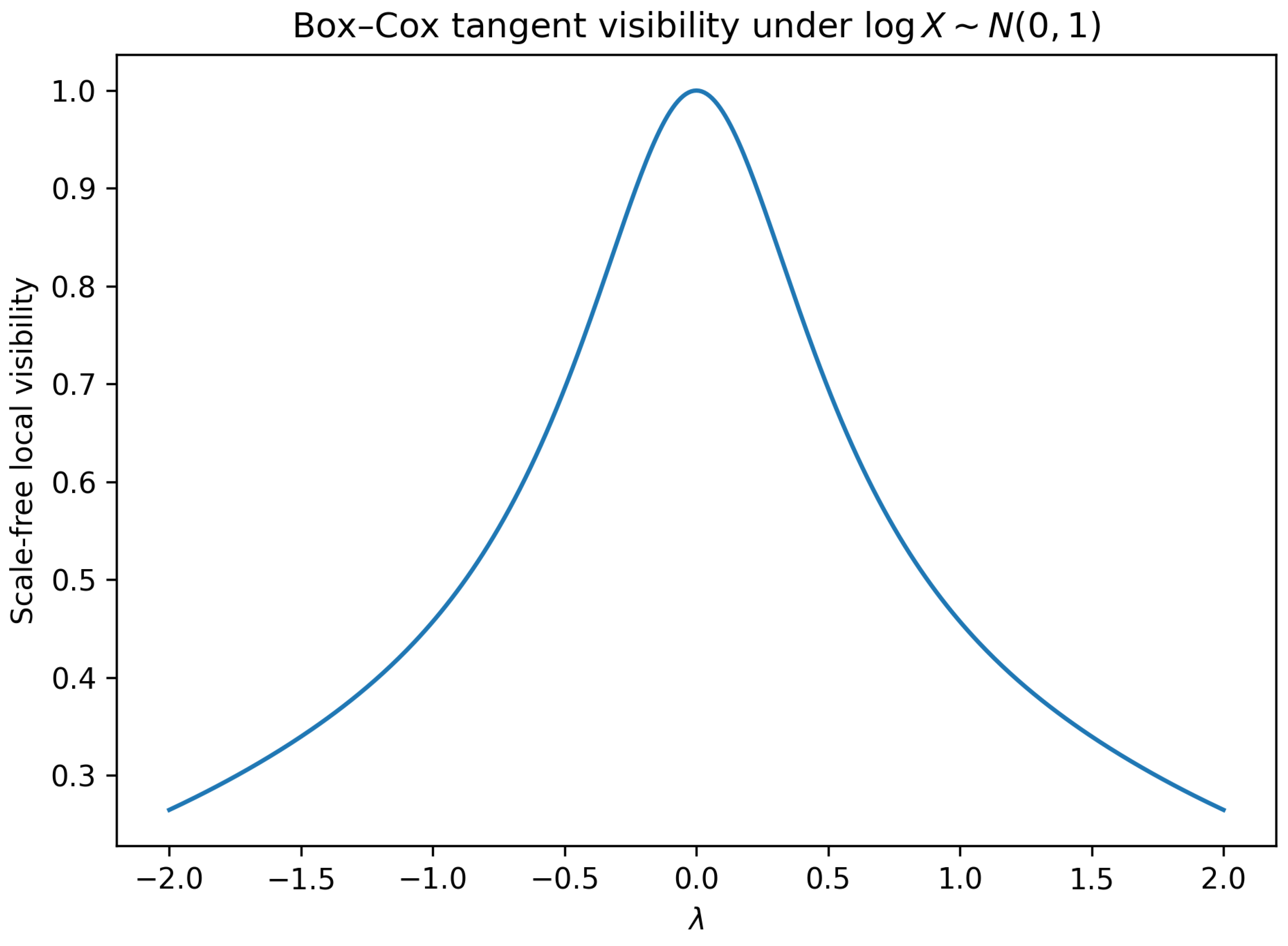
The profile is symmetric by construction because the closed-form expression depends on $\lambda$ only through $t={\lambda }^2$. Over $[-2,2]$, the scale-free visibility decreases from 1 at $\lambda =0$ to approximately $0.2647$ at $\left|\lambda \right|=2$. Thus, at $\left|\lambda \right|=2$, the residual norm is approximately $26.5\%$ of the norm of the centered tangent. Equivalently, since ${\nu }_{\mathrm{BC}}{\left(2\right)}^2\approx 0.0701$, about $7\%$ of the centered tangent variance remains outside its best affine approximation in the current Box–Cox scale.

Taken together, the analytical results show that local visibility depends strongly on both the functional direction and the position along the transformation path. These are local geometric properties of the criterion and do not, by themselves, imply global weak identification. Global weak identification depends on the geometry of the full correlation surface, in particular on the extent of its near-optimal region, and should therefore be assessed under a fully specified joint model or empirical design.

7. Discussion and Conclusions

The results clarify a structural limitation of correlation-based transformation selection. A high maximizing correlation value does not by itself imply sharp identification of the maximizing transformation parameter. The local sensitivity of Pearson correlation depends only on the component of the induced functional tangent that remains after projection onto $span\{1,U_{\theta }\}$. Affine components are invisible to the criterion, so transformations that differ substantially as functions may still be difficult to distinguish through standardized linear association alone.

This distinction is relevant in practice because correlation-based equivalence is weaker than transformation equivalence. Competing transformations may yield similar correlations while producing different marginal shapes, inverse-scale interpretations, or tail behaviour. Correlation maximization can therefore be a useful exploratory device, but selected parameters should be interpreted together with diagnostics of criterion stability, such as local visibility and near-optimal regions.

The analysis is general, but log-polynomial directions provide a natural local representation for the Box–Cox family through its expansion in powers of $logx$. The analytical illustrations show that visibility can vary markedly across these directions and along the Box–Cox path. Under the benchmark design, visibility is maximal at the logarithmic case and decreases substantially as $\left|\lambda \right|$ increases. This local information should not be conflated with global flatness of the objective: local sensitivity and global discrimination, as summarized for example by near-optimal regions, are complementary aspects of identification.

The paper does not propose correlation maximization as a substitute for likelihood-based inference. A correctly specified likelihood generally uses more information than Pearson correlation and may identify transformation parameters more strongly. The contribution here is instead to characterize what a correlation-based criterion can detect: to first order, it responds only to the non-affine component of transformation perturbations. This provides a geometric explanation for weak local discrimination whenever admissible parameter directions are nearly affine in the current transformed scale, and the pathwise bound shows how persistent low visibility can translate into weak discrimination over finite parameter regions.

Future work may extend the same projection-based framework to other location–scale invariant criteria, multivariate transformation families, and finite-sample versions of the visibility diagnostics.

References

- Box, G.E.P.; Cox, D.R. An Analysis of Transformations. J. R. Stat. Soc. Ser. B (Methodological) 1964, 26, 211–243. [Google Scholar] [CrossRef]
- Tukey, J.W. Exploratory Data Analysis; Addison-Wesley: Reading, MA, 1977. [Google Scholar]
- Yeo, I.K.; Johnson, R.A. A New Family of Power Transformations to Improve Normality or Symmetry. Biometrika 2000, 87, 954–959. [Google Scholar] [CrossRef]
- Rényi, A. On Measures of Dependence. Acta Math. Acad. Sci. Hung. 1959, 10, 441–451. [Google Scholar] [CrossRef]
- Breiman, L.; Friedman, J.H. Estimating Optimal Transformations for Multiple Regression and Correlation. J. Am. Stat. Assoc. 1985, 80, 580–598. [Google Scholar] [CrossRef]
- NIST/SEMATECH. Box–Cox Linearity Plot. E-Handb. Stat. Methods. Accessed. (accessed on 18 September 2026). [CrossRef]
- Filliben, J.J. The Probability Plot Correlation Coefficient Test for Normality. Technometrics 1975, 17, 111–117. [Google Scholar] [CrossRef]
- Lye, L.M. A Technique for Selecting the Box–Cox Transformation in Flood Frequency Analysis. Can. J. Civ. Eng. 1993, 20, 760–766. [Google Scholar] [CrossRef]
- Stock, J.H.; Wright, J.H.; Yogo, M. A Survey of Weak Instruments and Weak Identification in Generalized Method of Moments. J. Bus. Econ. Stat. 2002, 20, 518–529. [Google Scholar] [CrossRef]
- Andrews, D.W.K.; Cheng, X. Estimation and Inference With Weak, Semi-Strong, and Strong Identification. Econometrica 2012, 80, 2153–2211. [Google Scholar] [CrossRef]