

Submitted:
04 October 2026
Posted:
09 October 2026
You are already at the latest version
Abstract
The finite context window of a foundation model is the central scarce resource of an LLM agent harness: every token admitted costs money and latency and, beyond a point, degrades the answer. We argue that agent memory is an investment problem. What is written determines the retrieval problem the agent will later face, and the distribution of future retrievals determines what is worth writing. We formalize this as the joint optimization of a write policy (what is stored, at which resolution, with which shortcuts) and a read policy (what is loaded for a query) in one numeraire, with context tokens priced by a shadow price λ. We claim no novelty for the ingredients (value of information, submodular selection, rate–distortion, MDL, predictive information); The contribution is the coupling and what it implies: (i) a depth law in which optimal graph-traversal depth depends on token price, branching, signal decay and scorer quality; (ii) a write criterion measured against query-time re-derivation, with an explicit externality of writes on retrieval depth; (iii) a lower bound on the information content of any predictively sufficient memory; and (iv) thresholds for resolution levels, shortcuts, a cached core, query planning, refresh and indexing. Results are stated as propositions under explicit assumptions, design rules, and eight testable hypotheses. None is yet empirically validated.
Keywords:
agent memory
; context engineering
; information bottleneck
; knowledge graphs
; LLM agents
; predictive information
; retrieval-augmented generation
; token economics
; value of information
1. Introduction
An LLM agent is, architecturally, a harness around a function with a bounded input. The harness decides what the model sees, and the model can only reason over what lands in its context window. Even with windows of one million tokens, filling them indiscriminately is neither cheap nor effective: models recall less reliably as input grows [14], and position effects make the marginal value of a token depend on where it sits [13]. Practitioners summarize the goal as finding the smallest possible set of high-signal tokens that makes the desired outcome most likely [1]. This is a principle, not a theory.
Consider an agent whose persistent memory is a knowledge graph with attached evidence. When a query Q arrives, three questions arise. What is the optimal strategy to retrieve from the graph? What is the optimal strategy to build the graph? And what structure should the graph have so that retrieval is cheap? These are usually treated as separate engineering problems.
Thesis. Agent memory is an investment problem. Writing is an upfront expense that changes the future cost of access: a fact that is stored may save a later derivation, a summary makes later reads cheaper but lossy, a shortcut makes a recurring pattern cheap, and a fact that is stored adds branching that makes every later traversal more expensive. Conversely, the distribution of future queries determines which of these investments pay off. Write policy and read policy therefore cannot be optimized separately; they are two halves of one optimization over future information value.
Contributions. (1) We formulate write and read as a single bilevel problem in one numeraire, with a shadow price on context tokens (Section 3). (2) On the read side we derive local optimality conditions, a corrected statement of why the useful context size is bounded independently of the window, a depth law, and a value-of-information stopping rule with an explicit planner (Sections 5.1–5.3). (3) On the write side we derive an admission criterion measured against query-time re-derivation, quantify the externality a write imposes on retrieval depth, and prove a lower bound on the information content of a predictively sufficient memory (Sections 5.4–5.5). (4) For structure we derive rules for resolution levels, lazily built summaries, shortcuts, a cached core, refresh, and indexing versus lazy construction (Sections 5.6–5.8). (5) We state eight testable hypotheses (Section 6) and the limits of the theory (Section 7).
Status of claims. We separate three kinds of statements. Propositions are mathematical results that hold under the stated assumptions. Design rules are operational consequences of propositions, with the assumptions they inherit. Hypotheses are empirical predictions that have not been tested.
2. Related Work
Context engineering and token economics. Anthropic’s guidance on context engineering names the objective but offers no formalism [1]. A recent survey frames agent inference as cost minimization subject to a quality threshold, with shadow prices for tokens, and treats the context window as a rival resource [2]. It notes in a footnote that tokens differ in utility and information density, but its production function treats tokens as a homogeneous input. Our theory begins where that heterogeneity matters.
Agent memory systems. Temporal knowledge graphs [8], virtual-memory paging [9], extraction-and-consolidation pipelines [10], dynamically organized notes [27], hippocampus-inspired graph retrieval with personalized PageRank [28], and graph-indexed retrieval with multi-level search [29,7] are write-side or structure-side designs governed by heuristics. Hierarchical summary trees [30] build resolution levels. LongMemEval [31] evaluates extraction, multi-session and temporal reasoning, knowledge updates and abstention, but not cost. Notably, single-step graph retrieval has been reported to be 10–20 times cheaper than iterative LLM-driven retrieval [28], which already hints that the cost of retrieval lies in LLM calls, not in graph operations (Section 5.2).
Budgeted selection and learned retrieval. Greedy evidence selection by information gain per token [3], budgeted context construction with diversity constraints [4], prompt compression [32], and learned or adaptive retrieval policies [33,34] are read-side methods over flat chunks or fixed indexes.
Graph depth. Empirical studies report that retrieval performance peaks near depth three [5] and flow-based pruning applies per-hop decay with early stopping [6]. These are tuned heuristics without a dependence of the optimum on price, branching or scorer quality, and without a link to how the graph was built.
Classical theory. Table 1 lists the ingredients we draw on and what each leaves open.
Gap and claim. We claim no novelty for any single ingredient. The contribution is the coupling, and four things the synthesis yields that the ingredients do not: a price-dependent depth law (Eq. 3); a write criterion measured against query-time re-derivation, with an explicit externality of writes on retrieval depth (Eqs. 4, 6); a lower bound tying memory information content to predictive structure (Prop. 6); and one numeraire that prices every admission, placement, planning and refresh decision.
3. Problem Statement
3.1. The Scarcity
Context tokens are scarce in three senses. First, they have a price: money and latency per token. Second, their value is non-monotone: irrelevant tokens can reduce answer quality [13,14], so marginal value can be negative. Third, prices are tiered: tokens in a cached prefix cost a fraction of fresh tokens. A secondary scarcity is the write budget: tokens spent extracting, summarizing and maintaining the graph. Operations inside the graph store (joins, traversals, vector lookups) are a third, usually minor, cost, treated in Section 5.2.
3.2. Model
Definition 1 (Knowledge graph with evidence). A graph G stores a set of items (nodes, edges, evidence passages). Each item i is available at resolutions (e.g., gist, summary, full text, full text with detailed evidence) with token costs .
Definition 2 (Context and value). For a query with correct decision variable A, a context C is a set of (item, resolution) pairs with total token cost . Its value is : a relevant gain R (for log-loss utility, ) minus a distraction penalty that increases with the number of irrelevant tokens.
Definition 3 (Prices and numeraire). We express all costs in one utility numeraire. is the price of one fresh read token, of a cached prefix token, and of one write token (writes may use cheaper or batched models, so in general). Treating these as proportional is a modeling assumption, not a fact; the results below hold for any fixed ratios. At an optimum, equals the marginal value of a fresh read token.
Definition 4 (Policies). A write policy maps an observation stream to a graph G (including resolutions, shortcuts and a cached core). A read policy maps to a context C.
Objective. Let N be the number of queries the graph will serve and the tokens spent writing and maintaining it. The joint problem is
Because shapes the graph that sees, this is a bilevel problem: .
Assumptions. (A1) Queries are drawn i.i.d. from over the graph’s lifetime. (A2) R is monotone submodular and additive across traversal shells; is separable and increasing. (A3) Uniform contraction: the decision-relevant value available in the shell at distance h from the query’s entry points is at most with (Section 5.2). (A4) Predictive sufficiency: for results involving predictive information, the world is stationary and the stored graph is a sufficient statistic of the observation stream for the query-relevant future (Section 5.5).
4. The Pipeline
The theory addresses six stages of one pipeline (Figure 1).
5. Theory
5.1. Read: Selection
Proposition 1 (marginal-value conditions). Let and . (a) If V is additive over items with item values , the optimal context is . (b) In general, any local maximum C of F under single additions and removals satisfies
Proof. (a) maximizes term by term. (b) is the condition that no single addition or removal improves F. □
Part (b) is a necessary condition for local optimality, not a characterization of the global optimum, and it does not say that included items earn exactly . It does justify a best-first read policy: repeatedly add the item maximizing and stop when the ratio falls below . This is the marginal value theorem of optimal foraging [20]: leave a patch when the marginal rate of gain drops below the average rate.
Remark (approximation under a hard budget). If R is monotone submodular and the context is limited to a budget B, ratio-greedy combined with the best single item achieves a approximation [16], and partial enumeration achieves [17,15]. The distraction penalty makes V non-monotone, so these guarantees apply to the relevant-gain part only.
Proposition 2 (useful context size is bounded independently of the window). Let and . Let . (i) G is non-decreasing and constant for . (ii) Every maximizer of F satisfies . (iii) Let be the value of a policy that fills a budget B in decreasing order of relevant gain, ignoring distraction. If marginal relevant gain diminishes while marginal distraction cost is non-decreasing, then rises and then falls.
Proof. (i) The feasible sets are nested. (ii) From we get . (iii) The derivative of is marginal gain minus marginal distraction cost, which changes sign once. □
The optimal policy’s value never decreases with the window size W (it merely saturates), but a policy that fills the window does degrade. The practical content is that the optimal context has a finite size however large W is. Enlarging W beyond cannot help an optimal policy and can only hurt a filling one.
5.2. Read: Depth
Traversal depth is where the three-hop folklore lives. We derive its dependence on the economics.
Lemma 1 (signal decay; sufficient condition for A3). Suppose evidence about Q reaches node along a Markov chain whose hop channels have strong-data-processing contraction coefficients at most [25]. Then .
The data processing inequality alone gives only monotone decay [23]; geometric decay needs a uniform contraction coefficient, and graph traversal is not automatically such a chain (multiple paths between nodes can restore information). (A3) is therefore an assumption about the graph’s semantics, for instance chains of relations that lose specificity at each step, and is best treated as an effective parameter to be estimated.
Let the shell at distance h contain candidates of average token cost . Loading it without discrimination costs and yields value .
Proposition 3 (depth law). Under (A2) and (A3), shell h is worth loading iff , giving the optimal depth
Proof. Setting gives . Since , the ratio decreases in h, so all shells up to qualify. □
Example. With , , : . A depth-three optimum [5] is one point on a curve, not a constant.
Corollaries. (a) Cheaper tokens (smaller ) deepen the optimum, logarithmically. (b) Higher branching b reduces it. (c) A scorer that discriminates within a shell replaces b by an effective branching , so better rerankers deepen the optimum. (d) Materializing a recurring k-hop pattern as one edge (Section 5.6) removes hops from the effective depth. (e) Branching externality. Differentiating (3),
In the example, a 10% rise in average branching costs about hops. Every write that adds edges taxes all later traversals; Section 5.4 uses this.
Remark (non-token costs). Let be the cost, in the units of , of examining one node: a database lookup, a join step, an embedding comparison. With best-first expansion each loaded node entails at most about b examinations, so (3) holds with replaced by . Non-token costs are negligible iff .
Two orders of magnitude settle which case applies. A node of a hundred tokens at a few dollars per million input tokens costs a few hundredths of a cent, whereas a lookup or join step inside a database costs microseconds, many orders of magnitude less. Examination is not negligible when each examination is an LLM call (agentic scoring), because then (tokens of that call). The same holds for latency: a hop executed inside the database is nearly free, while a hop that needs an LLM decision costs a sequential round trip of seconds. The consistency of this picture with the reported 10–20 times cost gap between single-step graph retrieval and iterative LLM-driven retrieval [28] is suggestive but not a test.
Design rule D1. Execute graph hops inside the store and reserve LLM calls for decisions. The choice of store (relational with recursive queries, or a native graph database) matters through , latency tails at large fan-out, and the ability to express shortcuts, multi-resolution reads and temporal filters; it does not change the token economics.
5.3. Read: The Epistemic Layer and Planning
Relevance is not the right criterion; decision-sensitivity is. A cheap planner drafts the decision and its alternatives and identifies which unknowns the decision depends on.
Proposition 4 (myopic value-of-information stopping). Define
Fetching item i is single-step optimal iff , and myopic retrieval stops when no item satisfies this [18].
Value of information is classical; the point here is to use it as the retrieval criterion inside a persistent-memory system and to price it with the same that governs storage. Two cautions apply. First, the rule is myopic: VOI is not submodular, and complementary facts (a key and its lock) can each have zero VOI and a positive joint VOI, so myopic stopping can stop too early. Second, a known absence (“we checked; nothing exists”) has high VOI per token, so the graph should store confidence and absences explicitly.
Dependency analysis. Complementarity is exactly what dependency analysis finds. The planner builds a dependency graph of the query: which facts the decision depends on, and which fact identities depend on earlier fetched values. This is a backward slice from the decision [35], related to data provenance [36] and to query planning in databases [37]. Its structure determines the retrieval schedule. Independent branches can be fetched in parallel and evaluated as bundles (curing myopia). A chain of dependent lookups forces sequential rounds, so the dependency depth of the query, not only the traversal depth of the graph, sets the number of round trips. Shortcuts (Section 5.6) shorten graph paths; cached plan templates shorten dependency chains.
The same structure appears in epistemic foraging, where agents choose actions by expected information gain [38,39]. Decision-sensitivity differs from generic information gain in that information that cannot change the action has value zero.
Design rule D2 (plan only when it pays). Running the planner costs and is worthwhile iff its expected saving in retrieval cost and decision loss exceeds that cost. For recurring query types the plan is a reusable asset: caching a plan template for pattern r pays off under the same threshold as a shortcut (Proposition 8), with the cost of producing it.
5.4. Write: Admission
Retrieval is query-conditioned; writing is not. The write policy must decide, before the query is known, what to keep.
Proposition 5 (admission criterion). A candidate fact f should be written iff its expected lifetime read value, relative to the best query-time alternative, exceeds its write and maintenance cost:
where is computed with the best alternative available when f is absent (re-deriving it, calling a tool, asking the user), and , are the write and lifetime maintenance tokens.
By itself (6) is close to a tautology: expected benefit must exceed cost. Its content lies in how is computed, which gives three operational consequences.
Design rule D3 (write less). (a) Re-derivation. A fact that is cheap to re-derive at query time is not worth storing, however often it is asked. A fact that is expensive or impossible to re-derive, or whose loss is costly (high stakes, rarely queried), is worth storing even when rare. (b) Branching externality. A fact that adds to the average branching changes read value by roughly through Equation (4), so (6) can be violated by a fact that is individually useful but raises branching. (c) Redundancy. If for the query-relevant future Y, then and (6) rejects f. Storing everything is optimal only if every fact passes (6). This distinguishes the rule from storing everything, storing recent items, summarizing everything, and storing by embedding similarity.
5.5. Write: How Large Must Memory Be?
Proposition 6 (information lower bound, under A4). Let split the entropy of the observation stream into extensive and subextensive parts. The predictive information, the mutual information between past and future, equals [12]. Let be a memory state that is predictively sufficient, for the future Y. Then
If sufficiency is only required for query-relevant answer variables , the bound becomes , which is at most .
Proof. for discrete , and sufficiency gives equality with . □
For a world describable by K independent parameters, , and for nonparametric worlds it grows as with [12]. Two-part codes attain for regular parametric families [19], so in such worlds the bound is tight to leading order. Statistical complexity likewise bounds excess entropy from above in computational mechanics [40]; (7) is the same inequality in our setting.
Three qualifications keep this honest. (i) The result is about the description length of a sufficient memory, not the number of nodes: in a finite-parameter world the growth is in the precision of stored quantities, while the node count can stay constant. (ii) It is a lower bound; it does not say that any practical write policy attains it. (iii) It holds under (A4), which excludes non-stationarity (Section 5.7) and requires a sufficiency assumption that real graphs may not meet. Connecting this bound to admission, D3(c) shows that under (A4) criterion (6) never admits redundant facts, which pushes the admitted store toward a minimal sufficient statistic; we state this as a design consequence, not a theorem. Equation (7) defines value by predictive compression of the stream; Equation (6) defines it by future queries. They agree only when the query distribution is supported on the world’s predictive structure, which is the content of (A4).
5.6. Structure: Resolution, Summary Levels, Shortcuts, Cache
Proposition 7 (resolution choice, separable distortion). If the value lost at resolution ℓ is attributable to item i alone, with distortion relative to full evidence, the optimal resolution is
This is a rate–distortion tradeoff [24] with as the slope. With interacting facts the distortion becomes and (8) is only a heuristic. Resolution rises with relevance and falls with ; evidence-level resolution belongs to contested or high-stakes claims.
Design rule D4 (build summary levels lazily). Writing a summary level for item i costs about (read the item, write the summary). It saves on each retrieval at which the summary suffices. With lifetime retrievals, a sufficiency fraction , and expected content changes (each forcing a re-summary), the summary pays iff
When and , this is roughly : a leaf pays back its summary after one or two sufficient retrievals if its content is stable. Because is unknown at write time, the rule is implemented on read: generate the level when the observed retrieval count crosses the threshold in (9). Levels should be spaced roughly geometrically in token size (for example gist, summary, full, a factor of five to ten apart); this is a heuristic that follows from power-law distortion curves, not a theorem, and it implies few levels in practice. Internal summaries of subtrees or clusters serve a different purpose [30,7]: they give scent for deciding whether to descend, reducing the examined set from the branching fan-out to roughly summaries for n leaves at fan-out F (a saving on the examination cost of Section 5.2, not on the token side).
Proposition 8 (shortcut threshold). Suppose query patterns are Zipf-distributed over a fixed universe, with and stable normalizer H [22], and materializing pattern r as a one-hop edge saves tokens per query at a build and maintenance cost of tokens. The shortcut is worth building iff , i.e. for ranks
so the number of worthwhile shortcuts scales as . If the pattern universe itself grows with N, H is not constant and the exponent changes.
Proposition 9 (cached core). Place fact f in the cached prefix iff its inclusion probability across queries satisfies
where is its distraction cost when not needed.
Proof. A core item costs per query; fetching on demand costs . Compare. □
Example. With this reduces to . If cached tokens cost a tenth of fresh tokens, a fact used in more than roughly ten percent of queries belongs in the core. A cache-write surcharge raises the effective q in proportion to how often the prefix is rebuilt.
5.7. Time: Maintenance and Staleness
Facts change, and (A4) holds only for the stable part of the world. Let fact f have hazard rate , query rate , staleness stakes (the cost of answering from an outdated fact), and verification cost c. Assume a stationary hazard and a fixed query rate. The expected staleness probability averaged over a refresh interval T is , which is approximately for .
Proposition 10 (refresh interval, small hazard). For , re-verification every T minimizes , giving
Volatile, heavily queried, high-stakes facts are refreshed most often. For large the exact expression above must be minimized numerically. Bi-temporal validity windows [8] keep the changed state recoverable without discarding history.
5.8. Coupling: Why Write and Read Are One Problem
Indexing versus lazy construction. Let be the up-front cost of an index and the per-query token saving it provides over building context lazily at query time. Index iff
Below , lazy read-time construction (agentic search) is cheaper; above it, write-time indexing wins. With partial indexing, (10) determines which head patterns to index first.
Remark (joint versus separate). For any write policy , including one optimized without reference to retrieval (e.g., maximal stream compression), , since the joint optimum ranges over a superset. This is immediate and not the substantive claim. What is substantive is how large the gap is and where it comes from: the read-side parameters in (3) and (4) depend on the write policy. Summarization changes , shortcuts change the effective depth, fact admission changes b (Equation 4), and plan templates change the dependency depth. These are externalities of writing on reading, and they are the quantities Hypothesis 7 asks to measure.
A practical solution alternates: solve the read problem for the current graph, estimate per candidate fact, summary and shortcut from the query log, update the graph, and repeat. We make no convergence claim.
6. Hypotheses
The theory yields the following testable hypotheses; none is yet tested.
- 1.
- Depth is a function, not a constant. Optimal traversal depth follows (3): it grows with the log of the value-to-price ratio, falls with branching, and rises with scorer quality. A fixed depth of three is optimal only in a narrow parameter range.
- 2.
- Local marginal-value conditions. At a locally optimal context, the inequalities (2) hold: marginal gain per token of included items is at least and of excluded items at most .
- 3.
- Window size versus accuracy. A policy that stops by marginal value reaches a plateau as the window grows (Proposition 2), while a policy that fills the window peaks and then degrades; the peak lies near , independently of the window size.
- 4.
- Information growth in precision. For a predictively sufficient store in a finite-parameter domain, the stored information grows like in precision while node count saturates; in open-ended domains it grows as a power , . Fitting the growth curve diagnoses the regime. Raw logging grows linearly.
- 5.
- Shortcut scaling. The number of worthwhile shortcuts scales as with the Zipf exponent s of the query distribution (Equation 10).
- 6.
- Indexing threshold. Below queries, lazy construction dominates; above it, indexing does (Equation 13).
- 7.
- Write externality. Jointly optimized write–read policies beat independently tuned ones at equal total cost, and the measured sensitivity of optimal depth to branching approaches (Equation 4); the gap widens as queries concentrate (larger s).
- 8.
- Operational cost split. (a) With graph hops executed inside the store, the non-token cost share of a query is a small fraction of its token cost; it exceeds half only when each examination invokes an LLM. (b) Lazily built summaries break even after about retrievals, as in (9).
7. What This Theory Does Not Claim
- –
- It does not claim that knowledge graphs are always the best memory structure.
- –
- It does not claim that predictive information equals useful memory; Proposition 6 is a lower bound under a sufficiency assumption.
- –
- It does not claim that three-hop retrieval is universally wrong; it claims the optimum depends on measurable parameters.
- –
- It does not claim that the utility function of an LLM reader is known, or that , , and are easy to estimate.
- –
- It does not claim that the optimum is directly computable in production; the alternating procedure has no convergence guarantee.
- –
- It treats and the price ratios q and as given. A single numeraire is a modeling choice.
- –
- Its closed forms rest on stylized assumptions (geometric signal decay, submodular value, Zipf queries, stationary hazards) and should be read as derived consequences of those assumptions, not as laws.
References
- Rajasekaran, P.; Dixon, E.; Ryan, C.; Hadfield, J. Effective Context Engineering for AI Agents. Anthropic Engineering Blog, 2025. [Google Scholar]
- Chen, Y.; Chen, J.; He, C.; et al. Token Economics for LLM Agents: A Dual-View Study from Computing and Economics. arXiv 2026, arXiv:2605.09104. [Google Scholar]
- Enhancing Retrieval-Augmented Generation with Two-Stage Retrieval: FlashRank Reranking and Query Expansion. arXiv 2026, arXiv:2601.03258.
- Structure and Diversity Aware Context Bubble Construction for Enterprise Retrieval Augmented Systems. arXiv 2026, arXiv:2601.10681.
- Towards Open-World Retrieval-Augmented Generation on Knowledge Graph: A Multi-Agent Collaboration Framework. arXiv 2025, arXiv:2509.01238.
- Chen, B.; et al. PathRAG: Pruning Graph-based Retrieval Augmented Generation with Relational Paths. arXiv 2025, arXiv:2502.14902. [Google Scholar]
- Edge, D.; et al. From Local to Global: A Graph RAG Approach to Query-Focused Summarization. arXiv 2024, arXiv:2404.16130. [Google Scholar]
- Rasmussen, P.; Paliychuk, P.; Beauvais, T.; et al. Zep: A Temporal Knowledge Graph Architecture for Agent Memory. arXiv 2025, arXiv:2501.13956. [Google Scholar]
- Packer, C.; et al. MemGPT: Towards LLMs as Operating Systems. arXiv 2023, arXiv:2310.08560. [Google Scholar]
- Chhikara, P.; et al. Mem0: Building Production-Ready AI Agents with Scalable Long-Term Memory. arXiv 2025, arXiv:2504.19413. [Google Scholar]
- Tishby, N.; Pereira, F.C.; Bialek, W. The information bottleneck method. Proc. 37th Annual Allerton Conference on Communication, Control and Computing, 1999. [Google Scholar]
- Bialek, W.; Nemenman, I.; Tishby, N. Predictability, complexity, and learning. Neural Comput. 2001, 13(11), 2409–2463. [Google Scholar] [CrossRef]
- Liu, N.F.; et al. Lost in the Middle: How Language Models Use Long Contexts. Trans. ACL 2024, 12, 157–173. [Google Scholar] [CrossRef]
- Hong, K.; Troynikov, A.; Huber, J. Context Rot: How Increasing Input Tokens Impacts LLM Performance. Chroma Technical Report, 2025. [Google Scholar]
- Nemhauser, G.L.; Wolsey, L.A.; Fisher, M.L. An analysis of approximations for maximizing submodular set functions I. Math. Program. 1978, 14, 265–294. [Google Scholar] [CrossRef]
- Khuller, S.; Moss, A.; Naor, J. The budgeted maximum coverage problem. Inf. Process. Lett. 1999, 70(1), 39–45. [Google Scholar] [CrossRef]
- Sviridenko, M. A note on maximizing a submodular set function subject to a knapsack constraint. Oper. Res. Lett. 2004, 32(1), 41–43. [Google Scholar] [CrossRef]
- Howard, R.A. Information value theory. IEEE Trans. Syst. Sci. Cybern. 1966, 2(1), 22–26. [Google Scholar] [CrossRef]
- Rissanen, J. Modeling by shortest data description. Automatica 1978, 14(5), 465–471. [Google Scholar] [CrossRef]
- Charnov, E.L. Optimal foraging, the marginal value theorem. Theor. Popul. Biol. 1976, 9(2), 129–136. [Google Scholar] [CrossRef]
- Simon, H.A. Designing organizations for an information-rich world. In Computers, Communications, and the Public Interest; Greenberger, M., Ed.; Johns Hopkins Press, 1971; pp. 37–72. [Google Scholar]
- Zipf, G.K. Human Behavior and the Principle of Least Effort; Addison-Wesley, 1949. [Google Scholar]
- Cover, T.M.; Thomas, J.A. Elements of Information Theory, 2nd edn; Wiley, 2006. [Google Scholar]
- Shannon, C.E. Coding theorems for a discrete source with a fidelity criterion. IRE Nat. Conv. Rec. 1959, 4, 142–163. [Google Scholar]
- Ahlswede, R.; Gács, P. Spreading of sets in product spaces and hypercontraction of the Markov operator. Ann. Probab. 1976, 4(6), 925–939. [Google Scholar] [CrossRef]
- Bergmann, F.W. Functional Consciousness: A Proxy Metric Using Self-models (2026). In Artificial General Intelligence. AGI 2026. Lecture Notes in Computer Science(); Iklé, M., Franz, A., Kemendo, A., Lowy, H., Eds.; Springer: Cham; vol 16854. [CrossRef]
- Xu, W.; et al. A-MEM: Agentic Memory for LLM Agents. arXiv 2025, arXiv:2502.12110. [Google Scholar]
- Gutiérrez, B.J.; Shu, Y.; Gu, Y.; Yasunaga, M.; Su, Y. HippoRAG: Neurobiologically Inspired Long-Term Memory for Large Language Models. NeurIPS 2024, arXiv:2405.14831. [Google Scholar] [CrossRef]
- Guo, Z.; et al. LightRAG: Simple and Fast Retrieval-Augmented Generation. arXiv 2024, arXiv:2410.05779. [Google Scholar]
- Sarthi, P.; et al. RAPTOR: Recursive Abstractive Processing for Tree-Organized Retrieval. ICLR 2024, arXiv:2401.18059. [Google Scholar] [CrossRef]
- Wu, D.; et al. LongMemEval: Benchmarking Chat Assistants on Long-Term Interactive Memory. arXiv 2024, arXiv:2410.10813. [Google Scholar]
- Jiang, H.; et al. LLMLingua: Compressing Prompts for Accelerated Inference of Large Language Models; EMNLP, 2023. [Google Scholar]
- Asai, A.; et al. Self-RAG: Learning to Retrieve, Generate, and Critique through Self-Reflection. ICLR 2024, arXiv:2310.11511. [Google Scholar] [CrossRef]
- Jeong, S.; et al. Adaptive-RAG: Learning to Adapt Retrieval-Augmented Large Language Models through Question Complexity. NAACL 2024, arXiv:2403.14403. [Google Scholar] [CrossRef]
- Weiser, M. Program slicing. In Proc. 5th Int. Conf. on Software Engineering; IEEE, 1981; pp. 439–449. [Google Scholar]
- Buneman, P.; Khanna, S.; Tan, W.-C. Why and where: a characterization of data provenance. In ICDT 2001; Springer, 2001; Volume LNCS 1973, pp. 316–330. [Google Scholar]
- Selinger, P.G.; Astrahan, M.M.; Chamberlin, D.D.; Lorie, R.A.; Price, T.G. Access path selection in a relational database management system. In SIGMOD 1979; ACM, 1979; pp. 23–34. [Google Scholar]
- Pirolli, P.; Card, S. Information foraging. Psychol. Rev. 1999, 106(4), 643–675. [Google Scholar] [CrossRef]
- Friston, K.; et al. Active inference and epistemic value. Cogn. Neurosci. 2015, 6(4), 187–214. [Google Scholar] [CrossRef]
- Shalizi, C.R.; Crutchfield, J.P. Computational mechanics: pattern and prediction, structure and simplicity. J. Stat. Phys. 2001, 104, 817–879. [Google Scholar] [CrossRef]
Figure 1.
The write–read pipeline. One numeraire prices every admission, stopping, planning and placement decision.
Figure 1.
The write–read pipeline. One numeraire prices every admission, stopping, planning and placement decision.
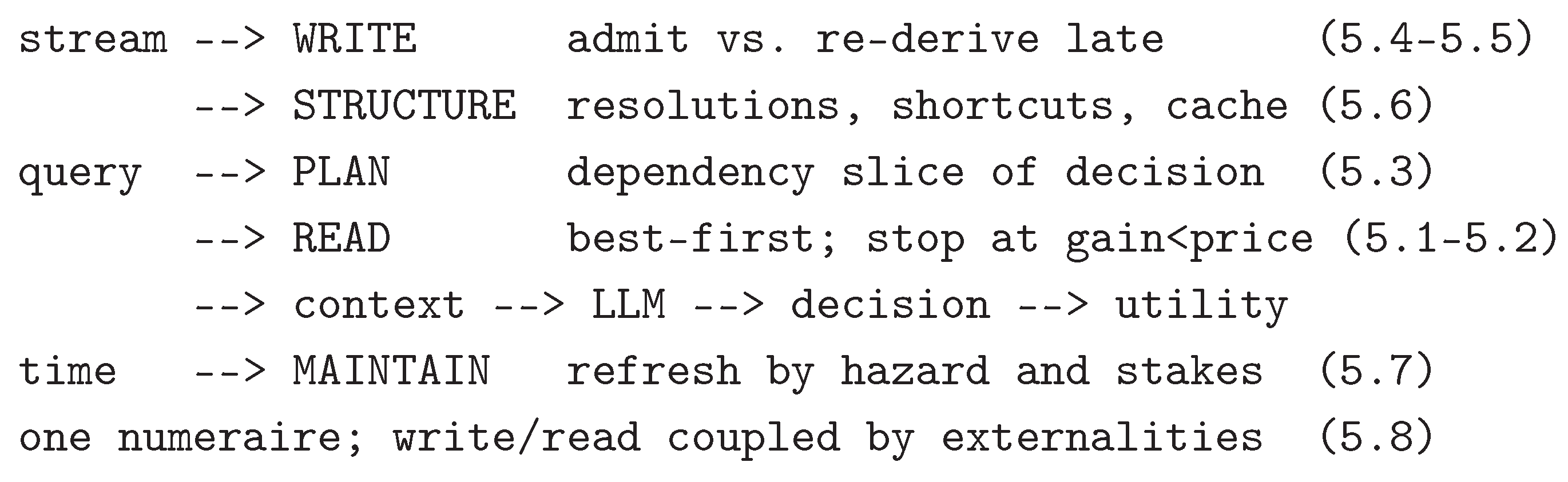

Table 1.
Ingredients and open questions.
| Theory | What it answers | What it leaves open |
|---|---|---|
| Value of information [18] | Is acquiring this fact worth its cost? | Persistent memory construction |
| Submodular selection [15–17] | Best set under a budget | How the candidate graph was built |
| Rate–distortion [24] | Fidelity versus size | Query-conditioned, graph-structured memory |
| MDL [19] | Compact model of the data | Value to future queries |
| Predictive information [12] | Learnable structure of a process | LLM context cost |
| Caching, inventory [2] | Repeated-access cost | Semantic, versioned memory |
| Graph-RAG [7,28,29] | Retrieval over structure | Principled write–read economics |
Disclaimer/Publisher’s Note: The statements, opinions and data contained in all publications are solely those of the individual author(s) and contributor(s) and not of MDPI and/or the editor(s). MDPI and/or the editor(s) disclaim responsibility for any injury to people or property resulting from any ideas, methods, instructions or products referred to in the content. |
© 2026 by the authors. Licensee MDPI, Basel, Switzerland. This article is an open access article distributed under the terms and conditions of the Creative Commons Attribution (CC BY) license (http://creativecommons.org/licenses/by/4.0/).
Copyright: This open access article is published under a Creative Commons CC BY 4.0 license, which permit the free download, distribution, and reuse, provided that the author and preprint are cited in any reuse.