

Submitted:
06 October 2026
Posted:
08 October 2026
You are already at the latest version
Abstract
Digital-twin research on additive-manufacturing (AM) fleets needs experi-ments in which the physical process, the communication channel and thetwin’s synchronisation state can be manipulated and measured indepen-dently; existing tools cover only fragments. SimTwin is an open-sourcePython simulator that couples a lumped-parameter thermal plant withproportional–integral heater control, a per-device job and health state ma-chine, an explicit message-level transport with latency, jitter, loss, dupli-cation, outage and staleness-based discarding, and a twin registry writtenonly by delivered messages. Faults are injected as mechanisms acting onthe plant, not as scripted telemetry labels, so fault signatures emerge fromthe dynamics, and seeding gives byte-identical telemetry. Seven experimentsreport scalability to 1 000 printers, throughput to 70 363 msg s−1, twin stale-ness rising from 0.99 s to 6.99 s with loss, 10 of 11 fault families separable atCohen’s |d| ≥ 1.45, and QoS 1 holding 95th-percentile staleness at 1.2 s on areal broker where QoS 0 lets it grow 12.6-fold.
Keywords:
digital twin
; additive manufacturing
; fused deposition modeling
; fleet simulation
; fault injection
; industrial IoT
; MQTT
; age of information
; reproducibility
1. Introduction
§2 positions the work, §4 gives the model and §3 the implementation, §4.8 the reproducibility contract, §6 the seven experiments, and §8–§9 what they mean, and what they do not.
Fused deposition modelling (FDM/FFF) fleets are becoming a networked, instrumented production setting: tens to hundreds of machines report telemetry over MQTT or OPC UA to a supervisory layer that maintains a digital twin of each machine (Grieves and Vickers, 2016; Tao et al., 2019; Barricelli et al., 2019; Fuller et al., 2020). The digital-twin literature is explicit that the value of a twin depends on the fidelity of the model, the freshness of its state, and the fidelity of the observed data (Tao et al., 2017; International Organization for Standardization, 2021,2), and that synchronisation is itself an engineering problem with a cost (Tan and Matta, 2023).
Research on this setting needs an experiment platform in which three things can be varied and measured independently: the physical process, the communication channel, and the twin’s synchronisation state. The tools that exist each cover one axis and assume the others away. Discrete-event factory simulators model queues and stations, not nozzle thermodynamics. Thermal and process models of a single extruder (Faria et al., 2020) model the physics in detail, for one machine, over an ideal channel. Networked-control-system studies model delay, dropout and scheduling (Walsh et al., 2002; Zhang et al., 2001) over an abstract plant. Age-of-information (AoI) work quantifies freshness of a source (Kaul et al., 2012; Yates et al., 2021) but has no process to be fresh about. AM fault-detection datasets are dominated by images and single-machine instrumented runs (Szydlo et al., 2021); predictive-maintenance benchmarks use machine-tool signals without a fleet, a network, or a twin.
This paper contributes SimTwin, a simulator built to close that gap, and the reproducible evidence base that comes with it.
Contributions
- 1.
- A layered architecture with a hard information barrier. Device state, twin-reported state, desired state, configuration and connectivity are separate objects. The twin registry is written only by messages the transport delivered, so twin staleness, synchronisation delay and resynchronisation counts are consequences of the channel model rather than annotations.
- 2.
- Mechanism-level fault injection. Eleven faults across five families are expressed as parameter transformations of the plant and observation models (Table 1). Fault signatures are emergent, which is what makes a separability study meaningful.
- 3.
- Explicit delivery semantics. Latency with a lognormal tail, independent loss, duplication, per-device disconnection with exponential reconnect backoff and replay queues, broker-wide outage, and staleness-based discarding, all applied in the transport, never in the device model.
- 4.
- Determinism by construction. A SeedPlan spawns independent named NumPy streams, so a run is a pure function of its configuration and seed. We verify this by hashing telemetry.
- 5.
- Seven experiments with published artifacts covering scalability, telemetry frequency, network impairment, fault separability, outage/recovery, reproducibility and broker fidelity, plus a dataset package with provenance metadata.
- 6.
- A fully verified bibliography: every journal, volume, issue, page range and DOI in this paper was resolved against the Crossref REST API; five candidate sources that could not be resolved were dropped (Section 8).
SimTwin is deliberately not a high-fidelity FDM physics simulator. It is a cyber-physical / industrial-IoT research testbed: the physics is the simplest lumped model that produces the qualitative behaviour the twin has to track, at a cost that lets a thousand-machine, hour-long scenario run on a laptop in under a minute.
2. Related Work
2.1. Digital Twins in Manufacturing
Grieves’ twin formulation separates the physical asset, its virtual model and the connections between them (Grieves and Vickers, 2016,1). Tao et al. formalise a five-layer architecture and the requirement for bidirectional coupling (Tao et al., 2019,1), and survey twin-driven smart-manufacturing system design (Liu et al., 2023). Standardisation has caught up: ISO 23247 defines a digital-twin framework for manufacturing (International Organization for Standardization, 2021) and ISO/IEC 30173 defines digital-twin representations of physical systems (International Organization for Standardization, 2023). Surveys map the enabling-technology landscape (Barricelli et al., 2019; Fuller et al., 2020), the maturity models used to classify twins (Uhlenkamp et al., 2022), and the methodologies by which twins are built (Aznar Lapuente et al., 2026). Reference architectures for synchronised twin factories are demonstrated in (Cho and Noh, 2024), and simulation-based twins for discrete material-flow systems in (Schwede and Fischer, 2024). The synchronisation problem—how far a twin may diverge from its physical twin, how that divergence is formulated, and what it costs to close the gap — is treated explicitly by Tan and Matta (2023). SimTwin is built to make that divergence measurable: it exposes per-twin age of information, synchronisation-delay percentiles, staleness and offline areas, and resynchronisation counts as first-class outputs.
2.2. AM/FDM Digital Twins and Process Simulation
Twin–AM integration is an active review area (Jyeniskhan et al., 2024). Machine-level twins have been demonstrated for FDM failure detection (Henson et al., 2021), for performance monitoring and anomaly detection in industry (Alhazmi et al., 2024), as a real-time twin ecosystem for AM (Pantelidakis et al., 2022), and as open-source reference implementations (Robles et al., 2023; Infante et al., 2025; Larsen et al., 2024). FIBR3DEmul is the closest physical analogue to SimTwin’s process layer: a multi-axis extrusion-deposition simulator for FDM (Faria et al., 2020). It targets bead geometry and material deposition for one machine; SimTwin targets fleet-level telemetry, connectivity and twin state, and uses a deliberately coarser deposition model (Section 4.3). Energy and resource accounting for AM is well established (Baumers et al., 2017; Wippermann et al., 2020); the SimTwin power model is an additive subsystem model in that tradition, calibrated to the order of magnitude of desktop FDM machines rather than fitted to a specific machine.
2.3. IIoT Transport, MQTT and Networked Control
MQTT (OASIS Standard, 2014,1) and OPC UA (Cavalieri and Cutuli, 2010) dominate IIoT messaging; publish/subscribe protocols for industrial settings are compared by Nast et al. (2022). Broker performance under load has been measured repeatedly (Mishra and Kertesz, 2020; Mishra et al., 2021; Silva et al., 2021), including CoAP/MQTT comparisons (Seoane et al., 2021), security-aware comparisons (Lakshminarayana et al., 2024), and MQTT-specific intrusion datasets (Alatram et al., 2023). MQTT in a twin data pipeline is demonstrated by Human et al. (2021), and the standards landscape for twin-enabled IoT by Jacoby and Usländer (2020). Networked control has a long literature on the control consequences of sampling, delay and dropout (Walsh et al., 2002; Zhang et al., 2001). Age-of-information gives the queueing-theoretic language for freshness (Kaul et al., 2012; Yates et al., 2021). SimTwin adopts the AoI view for the twin side and the dropout/delay view for the channel side, and puts both on top of a plant that produces the data.
2.4. Fault Detection, Anomaly Detection and Simulation Reporting
Model-based fault detection and diagnosis is the classical framework for residual generation from a physical model (Isermann, 2005). Data-driven anomaly detection supplies the statistics used to score fault separability here: local outlier factor (Breunig et al., 2000; Blázquez-García et al., 2021), isolation forests (Liu et al., 2008), one-class SVMs (Schölkopf et al., 2001), and deep approaches on AM process signals (Zamanzadeh Darban et al., 2024). Synthetic data is an established substitute for failure data that fleets do not generate in sufficient quantity (Nieminen et al., 2026); the published faulted-fleet dataset in Section 7 is offered in that spirit. Reporting guidelines for simulation-based research motivate the explicit treatment of seeds, environment capture and artifact publication in Section 7 (Rahmandad and Sterman, 2012).
2.5. Position of SimTwin
No prior open-source tool that we could verify combines (a) a per-device physical plant, (b) a finite-state job and health machine, (c) message-level network impairment with delivery semantics, (d) a twin registry whose state is derived only from delivered messages, and (e) mechanism-level fault injection with a published separability baseline. That combination, not the fidelity of any one layer, is the contribution.
3. System Architecture
The architecture realises the model of §4 as four cooperating parts: a vectorised plant, a twin registry, a transport, and a fault injector.
SimTwin is a Python 3 package (simtwin) organised as nine modules. The fleet engine (fleet/engine.py) is the integrator; everything else is a model it composes.
- config.py — thirteen dataclass configuration groups (experiment, fleet, simulation, thermal, power, material, job, health, network, twin, fault, storage, MQTT) with a validate() pass that rejects physically inconsistent parameter combinations before a run starts.
- printer/thermal.py — three coupled first-order thermal nodes (nozzle, bed, chamber) with PI heater control (Section 4.2).
- printer/process.py — additive subsystem power model, road-geometry deposition model, stochastic job generator (Section 4.3).
- printer/states.py — the device finite-state machine (Section 4.4).
- faults/catalogue.py, faults/injector.py — the fault catalogue and the scheduler that turns it into per-device parameter fields (Section 4.5).
- communication/message.py, communication/transport.py — the message model and the delivery-semantics pipeline (Section 4.6).
- twin/registry.py — the twin registry and synchronisation accounting (Section 4.7).
- storage/writers.py — CSV, JSONL and Parquet writers with environment and configuration provenance.
- metrics/quality.py — resource sampling and the separability statistics (Cohen’s d, Mann–Whitney AUC).
- utilities/seeds.py, utilities/environment.py — deterministic stream spawning and runtime environment capture.
The engine is vectorised: the fleet is a set of NumPy state arrays of length n, and one simulated timestep advances all devices with array operations. This is what makes a 1 000-machine, hour-long scenario a 51-second job (Section 6.1).
4. Model
4.1. Time Base
Time advances in steps of seconds (default 1 s). Telemetry is published every milliseconds (default 1 000 ms), and the transport is stepped every step, so delivery latencies finer than are represented by a continuous delivery-time distribution while the device state is sampled at the step grid. Configuration validation enforces ; experiments that need sub-second telemetry lower so that every interval is an integer multiple of the step (Section 6.2).
4.2. Thermal Plant
Each device has three lumped thermal nodes (nozzle, bed, chamber) with capacitance [J/K] and conductance to the ambient sink [W/K]:
where with duty , is a parasitic heat load, couples dissipation from the hot nodes into the chamber, and is an Ornstein–Uhlenbeck process with correlation time and stationary standard deviation —coloured, not white, process noise. Heaters are controlled by a saturating proportional–integral law on the measured temperature,
where is the sensor reading, so sensor bias and sensor noise enter the control loop exactly as they do on a real machine. Discretising (1) with step gives the update used by the engine, and (2) is integrated as a running sum per heater. The open-loop time constants at the defaults of Table 2 are s, s and s, and the full-power steady-state rises over ambient are K, K and K, which are the orders that make the setpoints 210/60/45 °C attainable with duty cycles in the interior of . The chamber heater is disabled by default: an open-frame desktop machine has no chamber heater, and the chamber warms by coupling.
4.3. Process, Power, Material and Jobs
Total electrical draw is an additive subsystem model,
with W standby, hot-end and part fans, a motion term scaling with normalised speed, and an extruder term; (3) is the quantity accumulated as energy use and compared against the nameplate rating in E4. Deposited volume follows the road geometry, for line width w, layer height h and print speed v; mass follows from filament density, and material use integrates over the print. Jobs are drawn from a generator with duration s, layer count , part volume mm3 and speed mm/s, with 5 % relative jitter on realised duration. Health accumulates wear at health-points per operating second, multiplied by the active fault’s wear multiplier; preventive maintenance is scheduled below a health of 0.35 and restores 0.92.
4.4. Device State Machine
Each device runs a finite-state machine over OFFLINE, IDLE, PREHEAT, PRINTING, PAUSED, COOLDOWN, FAILED and MAINTENANCE. Preheat completes when all enabled nodes are within 3K of setpoint for at least 20 s, and aborts as FAILED after 900 s. A terminal fault moves PRINTING → FAILED → MAINTENANCE, with repair time . The state machine is evaluated on the device side; the twin’s reported_state is a copy that arrives in a message.
4.5. Fault Mechanisms
This is the part of the simulator that E4 (§6.4) exercises directly. Faults are not telemetry labels. Each fault is a set of coefficients applied to the plant and observation models, ramped linearly from nominal to full severity over the fault’s ramp-in and back over its ramp-out, with severity drawn from the fault’s severity range. Table 1 lists the catalogue. Two faults are marked observational: they change only what the twin can observe, not the plant, which is what lets the evaluation distinguish a physical fault from a sensing fault. Faults are scheduled by a Poisson process at a configured rate per machine-hour, with per-family weights, and each injection is logged as an event with device, time, severity and duration.
4.6. Transport and Delivery Semantics
Every publication carries a generation timestamp, a kind (TELEMETRY, HEALTH, ALERTS, STATE, COMMAND, CONFIGURATION, LWT), a QoS level and a device id. The transport pipeline applies, in order:
- 1.
- Connectivity. Per-device disconnection episodes with mean interval and mean duration , with exponential reconnect backoff s at the k-th failed attempt; and broker-wide outage episodes.
- 2.
- Latency. plus a lognormal tail component with shape , so the bulk of the distribution is tight and the tail is heavy.
- 3.
- Loss. Independent per-message Bernoulli loss with probability p (QoS 0 semantics).
- 4.
- Duplication. With probability a QoS message is delivered twice (at-least-once semantics).
- 5.
- Replay. While a device is disconnected, its messages enter a bounded FIFO replay queue (limit ). Messages older than s at delivery are dropped as stale. Delivered replayed messages are flagged replayed.
All of this happens in the transport. The device model never learns that a message was lost, which is the point: a fault in the plant and a fault in the channel are separately attributable.
4.7. Twin Registry and Synchronisation Metrics
Each twin holds the reported state, the desired state, the confirmed configuration, the connectivity state, health, fault code, current job, progress, temperatures, power and material use, and the bookkeeping fields t_last_accepted, updates_accepted and resync_count. The only write path is apply(msg), called on delivery. From this we define, at simulated time t:
with s and s by default. Synchronisation delay is per accepted message, reported as mean and 95th/99th percentiles. Equation (4) defines the staleness whose percentiles are reported throughout §6; (5) defines the three-state classification whose counts give the stale and offline areas of (6), tabulated as twin_stale_area_s and twin_offline_area_s and reported per device so that they are comparable across fleet sizes. A resynchronisation is counted for each replayed telemetry message delivered after a disconnection, i.e. a reconnect recovery. Because the registry is write-only through delivery, all of these are measurements of the channel, not of the model’s self-report.
4.8. Determinism
A run is a pure function of (SimConfig, seed). SeedPlan derives independent numpy.random.Generator streams from a single SeedSequence for the job generator, thermal process noise, sensor noise, power noise, the fault scheduler, fault severities, connectivity, latency, loss, duplication and repair times. Spawning streams (rather than consuming one shared stream) means that adding a new stochastic source does not perturb the draws of the existing ones, which is what makes a scalability sweep and a fault sweep comparable across code changes.
5. Implementation and Artifacts
The package is pure Python with NumPy at the core; pandas, pyarrow, psutil, matplotlib, scipy, scikit-learn and paho-mqtt are used by the experiment, analysis and adapter layers. Storage writers emit CSV, JSONL and Parquet, and every run writes a metadata.json carrying the full resolved configuration, the seed, the fault summary, the artifact manifest, the metrics, and a captured environment record (OS, machine, CPU count, total memory, Python implementation and version, and the pinned versions of every dependency). An optional MQTT adapter (MqttTransport, MqttConfig, paho-mqtt 2.1.0) publishes the same Message objects on the same topics through a real broker, using separate publisher and subscriber clients so that messages genuinely leave the process and return, and registering a retained MQTT Last Will on the lwt topic so the registry learns of ungraceful disconnects without polling. The adapter is selected by a single configuration flag (mqtt.enabled); the fleet engine never branches on the transport type, and the adapter reports the same counter names as the in-process transport, so every metric and table works over either. Because the simulated clock runs hundreds of times faster than the wall clock, an asynchronous transport always has a backlog at the end of a run; the transport interface therefore includes an explicit flush that drains it at the final simulated time, so the tail of a run is attributed to latency rather than to loss. E7 (Section 6.7) exercises this adapter against Mosquitto 2.1.2. The unit-test suite contains 41 tests covering the thermal plant, the state machine, the fault injector, the transport, the MQTT adapter, the twin registry, determinism, storage round-trips and the metrics; the four MQTT tests skip themselves when no broker is listening.
6. Evaluation
Seven experiments, each stated as a question with a falsifiable expectation: §6.1 and §6.2 establish that the simulator is a credible instrument; §6.3 through §6.6 are the studies the instrument exists to make cheap; §6.7 checks the instrument against the real protocol. All experiments ran on a single Apple M3 Pro laptop (11 logical CPUs, 18 GiB RAM, Darwin 25.6.0, arm64), CPython 3.13.0, NumPy 2.5.3. No experiment uses more than one process. Table 2 gives the baseline parameters.
6.1. E1 — Scalability
Throughput peaks at device-steps s−1 around and falls to at ; the real-time factor (simulated seconds per wall-clock second) is 8 691 at and 88.6 at . The transition from a regime dominated by per-step fixed cost to one dominated by per-device array work is the expected signature of a vectorised engine, with the throughput decline beyond consistent with cache and memory pressure: peak resident set grows from 101 MB at to 3 289 MB at , i.e. MB per device, on a machine with 18 GiB. Delivery ratio is flat at 99.97 % across the sweep, confirming that the transport is not the scalability bottleneck at these sizes; the residual 0.03 % is the initial step, before any telemetry has been generated.
6.2. E2 — Telemetry Frequency
, duration 1 800 s, s (chosen so that every interval in the sweep is an integer multiple of the step), , 500, 1000, 5000, 10000, 30000, ms. Table 4 and Figure 2.
Delivered throughput spans 686 to 70 363 msg s−1, a factor of 102.5 across a 240-fold range of sampling periods; the shortfall from the ideal scaling at the finest settings is the 0.03 % initial-step loss plus queueing at the sink. Wall-clock time grows only from 4.37 s to 10.23 s over the same 240-fold range, i.e. a factor of 2.3: message generation and delivery is not the dominant cost of the simulation, the per-step plant update is. Peak RSS, by contrast, scales with the number of stored messages (703 MB at 60 s to 1 144 MB at 250 ms), which is the practical constraint on high-rate telemetry in long runs, and the reason the writers stream to Parquet.
6.3. E3 — Network Impairment
, duration 3 600 s. Sweep 1 varies loss . Sweep 2 varies the mean interval between per-device disconnection episodes, s with mean episode duration 60 s. Table 5 and Figure 3.
Loss. Delivery ratio tracks the ideal to within 0.05 percentage points at every setting, which is the correctness check for the loss model: 99.97 % at down to 70.05 % at . Mean transport latency is flat at 17.1 ms, as expected for independent per-message loss. The informative signal is freshness: 95th-percentile twin staleness grows from 0.99 s at to 6.99 s at , a slope of s per unit loss in the small-loss limit—each lost telemetry sample pushes the twin’s age of information out by one sampling period, which is the AoI result for a lossy periodic source (Kaul et al., 2012) reproduced by construction. The binary stale/offline counters stay at zero because the configured s is not crossed by loss alone at these rates; Section 6.5 shows the regime where they are.
Outages. Delivery ratio barely moves (99.97 % → 99.33 %) because replay recovers the buffered messages, while the twin-side cost explodes: mean synchronisation delay rises from 17 ms to 28 471 ms, offline area from 200 to 152 798 device·s, and resynchronisations from 0 to 324 942. This is the central twin-synchronisation finding of the paper: delivery and freshness are different quantities, and a replay mechanism protects the first while doing nothing for the second. A supervisory application that reads the twin and sees “99.3 % of messages arrived” would conclude the link is healthy; an application that reads twin staleness sees a fleet that is on average 179 s out of date.
6.4. E4 — Fault Injection and Separability
, duration 14 400 s (4 h), Poisson fault scheduling at 6 faults per machine-hour over the full catalogue, against a fault-free baseline at a different seed. 1 462 faults were injected across 11 types. For each fault type we compare telemetry samples recorded while the device was PRINTING with that fault active, against the fault-free PRINTING baseline, on seven channels: nozzle, bed and chamber temperature, power, print speed, cumulative material use, and health. We report Cohen’s d per channel and the Mann–Whitney AUC. Table 6 and Figure 4.
Every fault family separates from healthy printing on at least one channel with , which is “large” by Cohen’s conventions, and the separating channel is the mechanistically correct one. Bed-heater failure separates on power () because the controller saturates duty against a heater that no longer delivers heat. Motor overheating () and power anomaly () separate on power; nozzle-heater failure separates on nozzle temperature () with a compensating power rise; abnormal cooling separates on nozzle temperature (). The observational faults separate on health rather than on temperature mean, which is the signature of a sensing fault: the plant is untouched, so bed and chamber means barely move () while the wear accumulator, driven by fault severity, moves the health channel ( for sensor noise, for sensor drift).
The mean AUC across all seven channels sits at 0.42–0.50, i.e. near chance. That is not a failure of the model; it is the expected consequence of averaging a rank statistic over channels that a given fault does not touch, and it is the reason we report per-channel effect sizes. A detector that pools all channels will find nothing; a detector that looks at the mechanistically relevant channel finds a large, consistent separation. We read this as a concrete argument for mechanism-grounded feature selection in AM fault detection, and for publishing per-channel effect sizes rather than pooled scores.
6.5. E5 — Outage and Recovery
, duration 3 600 s, per-device disconnection episodes with mean interval 300 s and mean duration 60 s, with exponential reconnect backoff and replay queues. 235 disconnection and 218 reconnection events were recorded, producing 45 131 resynchronisations and 40 414 device·s of offline area. Median (over fleet samples) worst-twin staleness was 234 s with a maximum of 302 s, and mean synchronisation delay 27 982 ms with a maximum of 299 014 ms—the latter is the replay-queue age limit interacting with the backoff. Delivery ratio was 98.84 %.
The recovery behaviour is the interesting part. Because a reconnecting device sends a retained full-state snapshot before resuming telemetry, the twin converges to the device within one accepted message after each reconnection: the offline area is finite and the staleness distribution has a ceiling set by the episode duration plus backoff, not by the number of episodes. Without the snapshot, replay of a -message queue at 1 Hz would take longer than the run. This is the twin-side analogue of the last-will-and-testament plus retained-message pattern in MQTT 5 (OASIS Standard, 2019), and it is measurable here because the registry distinguishes delivered from generated. Table 7 gives the episode counts and the twin-side aggregates.
6.6. E6 — Reproducibility
Two runs at seed 2027 and one run at seed 2028, identical in every other respect. The two seed-2027 runs produce telemetry with identical SHA-256 digests (9e797bd1…965455); the seed-2028 run produces a different digest (995f11e1…b9a4cbd). Table 8. This is a strong form of reproducibility: bit-level identity of the artifact, not agreement of summary statistics to within a tolerance.
6.7. E7 — Broker Fidelity
Everything reported so far is produced by the in-process transport, so a natural question is whether that transport is an abstraction over a real one or a simulation of one. E7 answers this by running the same 20-device fleet, the same topic scheme, the same Message objects and the same QoS settings through a real Mosquitto 2.1.2 broker on loopback, using the adapter of Section 5. Table 9.
Three things are worth reading off the table. First, QoS 1 keeps the twin fresh and QoS 0 does not: at QoS 1 the mean observed delivery latency is 3.8 ms and twin staleness stays close to its telemetry-period floor at 1.2 s, while at QoS 0 the mean latency is 51,594 ms and p95 staleness rises to 15.1 s, a 12.6-fold degradation. The mechanism is back-pressure: QoS 1 blocks the publisher on PUBACK, which throttles the producer to the broker’s service rate, whereas QoS 0 is fire-and-forget, so a producer running hundreds of times faster than real time fills the client outbox and the twin observes a queue it cannot drain. This is the same phenomenon that E3 isolates parametrically, reproduced on real infrastructure.
Second, the broker path is lossless at both QoS levels, including at a configured loss of 0.30, because the underlying transport is TCP: the configured loss is an additive impairment the in-process model applies, not a property of the broker. The two transports therefore answer different questions — the in-process transport answers “what does a given impairment budget do to twin freshness?” and the broker transport answers “what does this broker actually do?” E3 and E7 should be read together, not averaged.
Third, the broker path is slower but not prohibitive: the QoS 1 broker run sustains an RTF of 156 against 445 for the in-process transport, i.e. a real broker round trip costs roughly two thirds of the headroom at this fleet size. Running a 1000-device study over a broker is feasible; running the full E1 sweep over a broker is not, which is why the scalability results use the in-process transport.
7. Dataset Package and Reproducibility
Each run directory contains telemetry.csv, telemetry.parquet, events.csv, twins.parquet (where written) and metadata.json. The metadata records the resolved configuration, the seed, the fault summary, the artifact manifest with per-file row counts, the run metrics, and the captured environment: OS release, machine and processor, logical CPU count, total memory, Python implementation and version, and the pinned versions of all ten dependencies (NumPy 2.5.3, pandas 3.0.6, pyarrow 25.0.1, psutil 7.2.2, matplotlib 3.11.2, scipy 1.18.1, scikit-learn 1.9.1, PyYAML 6.0.3, paho-mqtt 2.1.0, pytest 9.1.1). Per-experiment summary.csv files aggregate the sweeps, and results/bibliography_verification.{json,csv} records the Crossref resolution of every bibliography entry.
Reporting guidelines for simulation-based research (Rahmandad and Sterman, 2012) motivate three specific choices: an explicit warmup window excluded from analysis (60 s), a single seed per sweep point with the seed recorded in every summary row, and publication of the generating code alongside the data, so that a reader can regenerate any figure from the repository root with experiments/run_all.py followed by experiments/make_figures.py.
8. Threats to Validity and Limitations
Model fidelity. The thermal plant is a three-node lumped model with constant coefficients. It reproduces the qualitative behaviour a twin must track—setpoint tracking, first-order rise, saturating duty, the effect of a parasitic heat load—and it is calibrated to the order of magnitude of desktop FDM hardware, not fitted to any specific machine. It does not model melt-pool dynamics, layer-to-layer heat accumulation with temperature-dependent conductivity, convection that varies with part geometry, filament moisture, or crystallinity. Claims about bead geometry, residual stress, warping, or part strength are out of scope, and SimTwin should not be used for them. The deposition model is a road-geometry volume integral; it has no path planner.
Network fidelity. The transport models delivery semantics (latency, jitter, loss, duplication, disconnection, outage, replay, staleness) as independent stochastic mechanisms. It does not model bandwidth, contention, TCP congestion windows, TLS handshake cost, broker CPU, queueing at the broker, or the network stack of a real device. The reported msg/s figures are therefore the simulator’s own generation and delivery cost, not a broker’s capacity; broker capacity is measured against real brokers elsewhere (Mishra et al., 2021; Silva et al., 2021). The MQTT adapter lets a user replace the in-process bus with a real broker, and E7 exercises it, but only at : a broker round trip costs roughly two thirds of the simulator’s headroom (RTF 150 against 449), so the 1 000-device sweep in E1 could not be run over a broker in reasonable time. The scalability and fault results are therefore properties of the in-process transport, and E7 is the only result measured against real infrastructure.
Fault realism. Faults are parameter mechanisms with severity ranges drawn from engineering judgement, not from failure-mode data fitted to a fleet. The separability result shows that the injected mechanisms produce signatures that are large and mechanistically coherent; it does not show that real FDM faults have those magnitudes. The 11-fault catalogue is a starting point, not a taxonomy of FDM failure. One catalogue fault (print_interruption) is terminal and short-lived, so it produced fewer than 30 qualifying PRINTING samples and is absent from Table 6; its effect is on job outcomes, not on telemetry distributions.
Statistics. Each sweep point is a single seeded run, not a set of replicates, so the sweeps carry no confidence intervals. The determinism result (E6) makes this a deliberate, reproducible choice rather than an accident, and the separability statistics in E4 are computed over – samples per fault, which is ample for the rank-based statistics used. Effect sizes, not hypothesis tests, are the reported quantity.
Timing variance. The simulated physics is exactly reproducible; the wall-clock columns are not. They are single measurements on a general purpose laptop, and re-running the same configuration on the same machine moves them by ten to twenty per cent with background load — the E1 point has been observed at both 70 611 and 88 643 device-steps s−1, and the E7 QoS 0 staleness figure at both 13.2 s and 15.1 s, on identical configurations and seeds. The reported figures are from the final full-suite run, whose generating code, configuration and seeds are all published. Scalability trends — the peak near , the linear RSS growth, the monotone staleness response — are stable across runs; the absolute constants are indicative, not certified, and any comparison against them should be made on the same hardware under comparable load.
Scope of the evidence. The largest fleet is 1 000 devices for one simulated hour. We do not claim behaviour at devices, over multi-day horizons, or under the memory pressure that a long high-rate telemetry run on a smaller machine would produce.
Bibliography. Every entry in this paper was resolved against the Crossref REST API. Five candidate sources—a networked-control survey, a predictive-maintenance dataset paper, and three AM-energy papers—could not be resolved to the works described at any DOI we could verify, and were dropped rather than cited with an unverifiable identifier. Several further entries had a resolvable DOI but a year, first author or journal attribution that Crossref contradicted, and were corrected to the resolved record (Grieves and Vickers, 2016; Liu et al., 2023; Baumers et al., 2017). The machine-readable audit is published with the artifacts.
9. Conclusions
The three findings of §6—that delivery and freshness diverge, that fault signal is per-channel, and that determinism is a property of the composition rather than of any one module—are the reason this simulator is worth building on.
We presented SimTwin, an open-source, deterministic, mechanism-level simulator of networked FDM/FFF fleets that couples a physical plant, a job and health state machine, a message-level transport with explicit delivery semantics, and a twin registry whose state is derived only from delivered messages. The evaluation establishes that the tool runs at useful scale on commodity hardware, that its channel model reproduces the analytic loss and age-of-information behaviour it is meant to represent, that delivery and freshness are measurably different quantities under outage, and that injected fault mechanisms produce large, mechanistically coherent, per-channel separability from healthy operation. The artifact—source, tests, experiment scripts, per-run metadata, summary tables, figures and a Crossref-verified bibliography—is published as a package, and every figure in this paper can be regenerated from the repository root by two commands.
Future work follows directly from the limitations: fitting the thermal and fault parameters against instrumented machines; coupling the transport to a real broker and measuring the delta; adding replicates and reporting confidence intervals; extending the fault catalogue from failure-mode data; and using the twin synchronisation metrics as an explicit objective in a scheduling or edge-offloading study.
Author Contributions
N.S.: Conceptualization, Methodology, Software, Validation, Formal analysis, Investigation, Writing—original draft, Writing—review & editing, Visualization. A.K.: Conceptualization, Software, Validation, Investigation, Writing—review & editing, Resources.
Funding
This research did not receive any specific grant from funding agencies in the public, commercial, or not-for-profit sectors.
Data Availability Statement
The SimTwin package, the experiment scripts (experiments/run_all.py, experiments/make_figures.py), the unit-test suite, the per-run artifacts, the summary tables, the figures and the bibliography verification audit are published together in the project repository. Running pythonexperiments/run_all.py regenerates every result, and pythonexperiments/make_figures.py regenerates every figure and every table in this paper. The simulator source, the experiment drivers, the per-experiment result tables, the dataset manifest and the bibliography-verification records are released at https://github.com/Okami29/simtwin (tag v0.1.1) and archived with a persistent identifier on Zenodo. Every figure and table in this paper is generated from that archived artefact by the scripts in experiments/, and all runs are seeded, so every number reported here can be regenerated from the deposited configurations.
Acknowledgments
Machine-assisted tooling was used for literature retrieval, Crossref verification scripting, code scaffolding and drafting support. All scientific decisions, model design, experiment design, interpretation and the final bibliography audit are the authors’ responsibility, and every citation was verified against Crossref as described in Section 8.
Conflicts of Interest
N.S. is co-founder and Chief Technology Officer of G3D LLC, a 3D-printer and additive-manufacturing company, and founder of Versec LLC, an automation and technology-development studio. A.K. is affiliated with G3D LLC. G3D manufactures the class of FDM/FFF equipment that SimTwin models, so the authors have a professional interest in the adoption of the tool and a financial interest in a company that may benefit from it. Against this: SimTwin models generic FDM/FFF kinematics and thermodynamics and depends on no proprietary G3D hardware, design data or trade secret; the simulator, experiment drivers and all result tables are released under the MIT licence; every figure and table in this paper is regenerated from the deposited artefacts; and no qualitative conclusion reported here changes if the G3D-derived parameter defaults are replaced by the generic defaults documented in the configuration files. The authors declare no other competing financial interest.
References
- Grieves, M., and J. Vickers. 2016. Digital Twin: Mitigating Unpredictable, Undesirable Emergent Behavior in Complex Systems. In Transdisciplinary Perspectives on Complex Systems. Springer International Publishing: pp. 85–113. [Google Scholar] [CrossRef]
- Tao, F., H. Zhang, A. Liu, and A.Y.C. Nee. 2019. Digital Twin in Industry: State-of-the-Art. IEEE Trans. Ind. Inform. 15: 2405–2415. [Google Scholar] [CrossRef]
- Barricelli, B.R., E. Casiraghi, and D. Fogli. 2019. A Survey on Digital Twin: Definitions, Characteristics, Applications, and Design Implications. IEEE Access 7: 167653–167671. [Google Scholar] [CrossRef]
- Fuller, A., Z. Fan, C. Day, and C. Barlow. 2020. Digital Twin: Enabling Technologies, Challenges and Open Research. IEEE Access 8: 108952–108971. [Google Scholar] [CrossRef]
- Tao, F., J. Cheng, Q. Qi, M. Zhang, H. Zhang, and F. Sui. 2017. Digital twin-driven product design, manufacturing and service with big data. Int. J. Adv. Manuf. Technol. 94: 3563–3576. [Google Scholar] [CrossRef]
- International Organization for Standardization. 2021. ISO 23247-1:2021. Automation Systems and Integration — Digital Twin Framework for Manufacturing: Part 1, Overview and General Principles Standard. no DOI assigned.
- International Organization for Standardization. 2023. ISO/IEC 30173:2023. Information Technology — Digital Twin — Concepts and Terminology Standard. no DOI assigned.
- Tan, B., and A. Matta. 2023. The digital twin synchronization problem: Framework, formulations, and analysis. IISE Trans. 56: 652–665. [Google Scholar] [CrossRef]
- Faria, C., J. Fonseca, and E. Bicho. 2020. FIBR3DEmul—an open-access simulation solution for 3D printing processes of FDM machines with 3+ actuated axes. Int. J. Adv. Manuf. Technol. 106: 3609–3623. [Google Scholar] [CrossRef]
- Walsh, G., H. Ye, and L. Bushnell. 2002. Stability analysis of networked control systems. IEEE Trans. Control Syst. Technol. 10: 438–446. [Google Scholar] [CrossRef]
- Zhang, W., M.S. Branicky, and S.M. Phillips. 2001. Stability of networked control systems. IEEE Control Syst. Mag. 21: 84–99. [Google Scholar] [CrossRef]
- Kaul, S., R. Yates, and M. Gruteser. 2012. Real-time status: How often should one update? In Proceedings of the 2012 Proceedings IEEE INFOCOM. IEEE: pp. 2731–2735. [Google Scholar] [CrossRef]
- Yates, R.D., Y. Sun, D.R. Brown, S.K. Kaul, E. Modiano, and S. Ulukus. 2021. Age of Information: An Introduction and Survey. IEEE J. Sel. Areas Commun. 39: 1183–1210. [Google Scholar] [CrossRef]
- Szydlo, T., J. Sendorek, M. Windak, and R. Brzoza-Woch. 2021. Dataset for Anomalies Detection in 3D Printing. In Lecture Notes in Computer Science. Springer International Publishing: pp. 647–653. [Google Scholar] [CrossRef]
- Grieves, M., and J. Vickers. 2014. Digital Twin: Manufacturing Excellence through Virtual Factory Replication. In White paper. White paper; no DOI assigned. Melbourne, FL, USA: Florida Institute of Technology. [Google Scholar]
- Liu, S., P. Zheng, and J. Bao. 2023. Digital Twin-based manufacturing system: a survey based on a novel reference model. J. Intell. Manuf. 35: 2517–2546. [Google Scholar] [CrossRef]
- Uhlenkamp, J.F., J.B. Hauge, E. Broda, M. Lutjen, M. Freitag, and K.D. Thoben. 2022. Digital Twins: A Maturity Model for Their Classification and Evaluation. IEEE Access 10: 69605–69635. [Google Scholar] [CrossRef]
- Aznar Lapuente, G., P. Morella Avinzano, M.P. Lamban Castillo, and D. Seneviratne. 2026. Methodologies in digital twin for manufacturing industry: A systematic literature review. Future Gener. Comput. Syst. 174: 107997. [Google Scholar] [CrossRef]
- Cho, Y., and S.D. Noh. 2024. Design and Implementation of Digital Twin Factory Synchronized in Real-Time Using MQTT. Machines 12: 759. [Google Scholar] [CrossRef]
- Schwede, C., and D. Fischer. 2024. Learning Simulation-Based Digital Twins for Discrete Material Flow Systems: A Review. In Proceedings of the 2024 Winter Simulation Conference (WSC). IEEE: pp. 3070–3081. [Google Scholar] [CrossRef]
- Jyeniskhan, N., K. Shomenov, M.H. Ali, and E. Shehab. 2024. Exploring the integration of digital twin and additive manufacturing technologies. Int. J. Lightweight Mater. Manuf. 7: 860–881. [Google Scholar] [CrossRef]
- Henson, C.M., N.I. Decker, and Q. Huang. 2021. A digital twin strategy for major failure detection in fused deposition modeling processes. Procedia Manuf. 53: 359–367. [Google Scholar] [CrossRef]
- Alhazmi, T., F. Azzedin, and M. Hammoudeh. MQTT Based Data Distribution Framework for Digital Twin Networks. Proceedings of the Proceedings of the 8th International Conference on Future Networks & Distributed Systems, 2024; ACM, pp. 1008–1013. [Google Scholar] [CrossRef]
- Pantelidakis, M., K. Mykoniatis, J. Liu, and G. Harris. 2022. A digital twin ecosystem for additive manufacturing using a real-time development platform. Int. J. Adv. Manuf. Technol. 120: 6547–6563. [Google Scholar] [CrossRef] [PubMed]
- Robles, J., C. Martín, and M. Díaz. 2023. OpenTwins: An open-source framework for the development of next-gen compositional digital twins. Comput. Ind. 152: 104007. [Google Scholar] [CrossRef]
- Infante, S., J. Robles, C. Martín, B. Rubio, and M. Díaz. 2025. Distributed digital twins on the open-source OpenTwins framework. Adv. Eng. Inform. 64: 102970. [Google Scholar] [CrossRef]
- Larsen, L., T. Fraunholz, T. Köhler, D. Rall, V. Langner, D. Görick, and A. Schuster. 2024. RECAST: An Open-Source Digital Twin Framework for Industrial Production Environments. In Lecture Notes in Mechanical Engineering. Springer Nature Switzerland: pp. 160–171. [Google Scholar] [CrossRef]
- Baumers, M., J.R. Duflou, W. Flanagan, T.G. Gutowski, K. Kellens, and R. Lifset. 2017. Charting the Environmental Dimensions of Additive Manufacturing and 3D Printing. J. Ind. Ecol. 21. [Google Scholar] [CrossRef]
- Wippermann, A., T.G. Gutowski, B. Denkena, M.A. Dittrich, and Y. Wessarges. 2020. Electrical energy and material efficiency analysis of machining, additive and hybrid manufacturing. J. Clean. Prod. 251: 119731. [Google Scholar] [CrossRef]
- OASIS Standard. 29 October 2014, 2014. MQTT Version 3.1.1. OASIS Standard, Industry specification; no DOI assigned.
- OASIS Standard. 3 December 2019, 2019. MQTT Version 5.0. OASIS Standard, Industry specification; no DOI assigned.
- Cavalieri, S., and G. Cutuli. 2010. Performance evaluation of OPC UA. In Proceedings of the 2010 IEEE 15th Conference on Emerging Technologies & Factory Automation (ETFA 2010). IEEE: pp. 1–8. [Google Scholar] [CrossRef]
- Nast, M., H. Raddatz, B. Rother, F. Golatowski, and D. Timmermann. A Survey and Comparison of Publish/Subscribe Protocols for the Industrial Internet of Things (IIoT). Proceedings of the Proceedings of the 12th International Conference on the Internet of Things, 2022; ACM, pp. 193–200. [Google Scholar] [CrossRef]
- Mishra, B., and A. Kertesz. 2020. The Use of MQTT in M2M and IoT Systems: A Survey. IEEE Access 8: 201071–201086. [Google Scholar] [CrossRef]
- Mishra, B., B. Mishra, and A. Kertesz. 2021. Stress-Testing MQTT Brokers: A Comparative Analysis of Performance Measurements. Energies 14: 5817. [Google Scholar] [CrossRef]
- Silva, D., L.I. Carvalho, J. Soares, and R.C. Sofia. 2021. A Performance Analysis of Internet of Things Networking Protocols: Evaluating MQTT, CoAP, OPC UA. Appl. Sci. 11: 4879. [Google Scholar] [CrossRef]
- Seoane, V., C. Garcia-Rubio, F. Almenares, and C. Campo. 2021. Performance evaluation of CoAP and MQTT with security support for IoT environments. Comput. Netw. 197: 108338. [Google Scholar] [CrossRef]
- Lakshminarayana, S., A. Praseed, and P.S. Thilagam. 2024. Securing the IoT Application Layer From an MQTT Protocol Perspective: Challenges and Research Prospects. IEEE Commun. Surv. Tutor. 26: 2510–2546. [Google Scholar] [CrossRef]
- Alatram, A., L.F. Sikos, M. Johnstone, P. Szewczyk, and J.J. Kang. 2023. DoS/DDoS-MQTT-IoT: A dataset for evaluating intrusions in IoT networks using the MQTT protocol. Comput. Netw. 231: 109809. [Google Scholar] [CrossRef]
- Human, C., A.H. Basson, and K. Kruger. 2021. Digital Twin Data Pipeline Using MQTT in SLADTA. In Studies in Computational Intelligence. Springer International Publishing: pp. 111–122. [Google Scholar] [CrossRef]
- Jacoby, M., and T. Usländer. 2020. Digital Twin and Internet of Things—Current Standards Landscape. Appl. Sci. 10: 6519. [Google Scholar] [CrossRef]
- Isermann, R. 2005. Model-based fault-detection and diagnosis – status and applications. Annu. Rev. Control 29: 71–85. [Google Scholar] [CrossRef]
- Breunig, M.M., H.P. Kriegel, R.T. Ng, and J. Sander. LOF. Proceedings of the Proceedings of the 2000 ACM SIGMOD international conference on Management of data, 2000; ACM, pp. 93–104. [Google Scholar] [CrossRef]
- Blázquez-García, A., A. Conde, U. Mori, and J.A. Lozano. 2021. A Review on Outlier/Anomaly Detection in Time Series Data. ACM Comput. Surv. 54: 1–33. [Google Scholar] [CrossRef]
- Liu, F.T., K.M. Ting, and Z.H. Zhou. 2008. Isolation Forest. In Proceedings of the 2008 Eighth IEEE International Conference on Data Mining. IEEE: pp. 413–422. [Google Scholar] [CrossRef]
- Schölkopf, B., J.C. Platt, J. Shawe-Taylor, A.J. Smola, and R.C. Williamson. 2001. Estimating the Support of a High-Dimensional Distribution. Neural Comput. 13: 1443–1471. [Google Scholar] [CrossRef] [PubMed]
- Zamanzadeh Darban, Z., G.I. Webb, S. Pan, C. Aggarwal, and M. Salehi. 2024. Deep Learning for Time Series Anomaly Detection: A Survey. ACM Comput. Surv. 57: 1–42. [Google Scholar] [CrossRef]
- Nieminen, W., H. Gebreweld, A. Liuha, M. Nissinen, M. Verdugo, A. Mikkola, and A. Kutvonen. 2026. Synthetic Data for Predictive Maintenance: A Systematic Review and Framework for Industry 4.0 Applications. J. Intell. Manuf. [Google Scholar] [CrossRef]
- Rahmandad, H., and J.D. Sterman. 2012. Reporting guidelines for simulation-based research in social sciences. Syst. Dyn. Rev. 28: 396–411. [Google Scholar] [CrossRef]
Figure 1.
E1 scalability on a single 11-core laptop. (a) Device-steps/s and telemetry msg/s both peak near and decline gently at ; (b) wall-clock time grows linearly in n (dotted reference: device-steps); (c) peak resident set grows linearly at MB per device (dotted reference: ). All axes logarithmic.
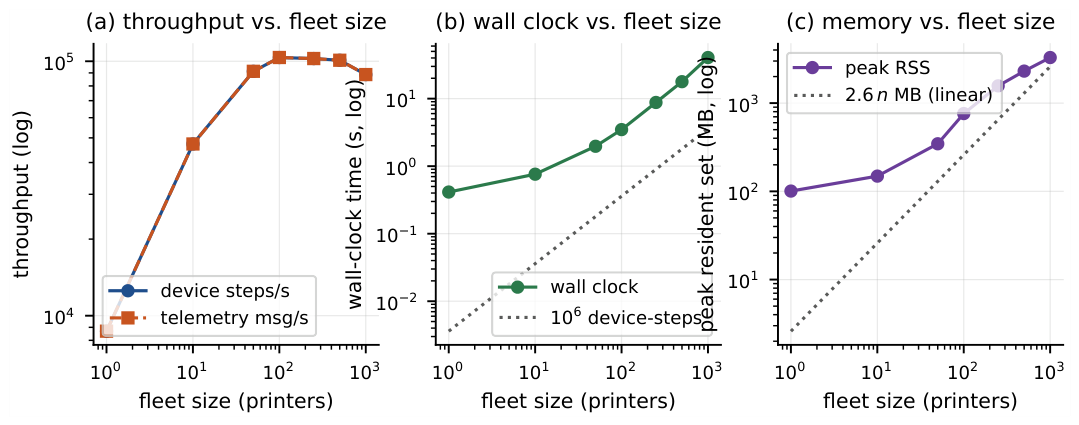
Figure 2.
E2 telemetry frequency. (a) Delivered and generated message rates track over 2.4 orders of magnitude; (b) the wall-clock cost of the same sweep changes by only a factor of 2.4, so the plant update, not the messaging, dominates.
Figure 2.
E2 telemetry frequency. (a) Delivered and generated message rates track over 2.4 orders of magnitude; (b) the wall-clock cost of the same sweep changes by only a factor of 2.4, so the plant update, not the messaging, dominates.
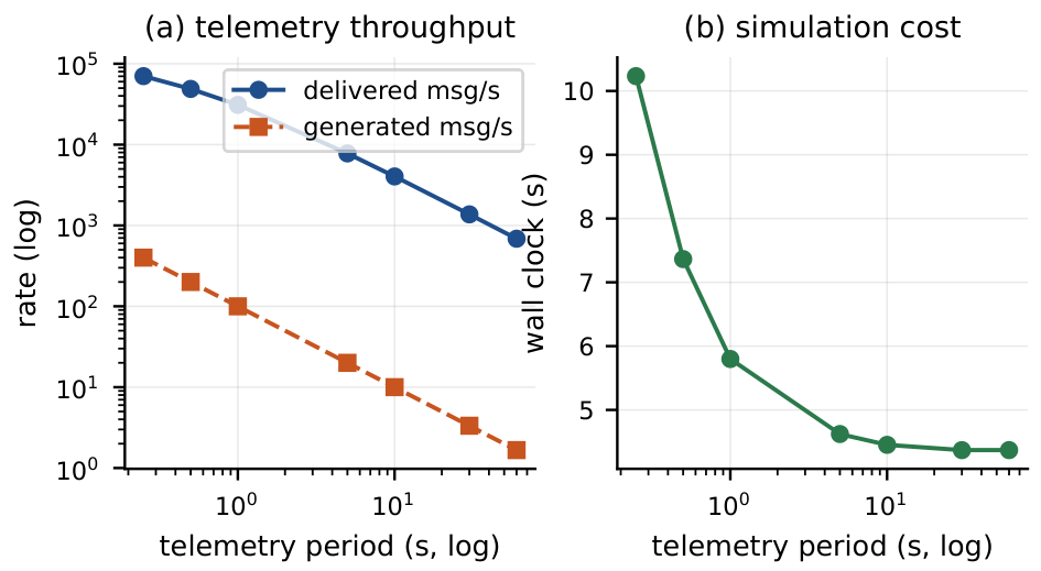
Figure 3.
E3 network impairment. (a) Delivery ratio follows the ideal while 95th-percentile twin staleness grows linearly in loss; (b) increasing outage frequency leaves delivery near-perfect while offline area and resynchronisation counts grow by five orders of magnitude.
Figure 3.
E3 network impairment. (a) Delivery ratio follows the ideal while 95th-percentile twin staleness grows linearly in loss; (b) increasing outage frequency leaves delivery near-perfect while offline area and resynchronisation counts grow by five orders of magnitude.
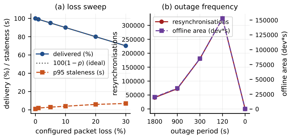
Figure 4.
E4 fault separability. Per-channel Cohen’s d between faulted and healthy printing telemetry, ordered by largest absolute effect. The structure is mechanistic: thermal-actuator faults move temperature and power, power-domain faults move power, and observational faults move health while leaving temperature means near-unchanged.
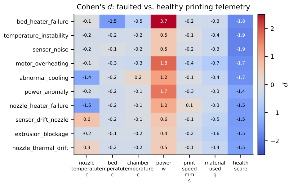

Table 1.
Fault catalogue. Coefficients are the values reached at full severity. Term. marks a fault that aborts the active job; Obs. marks a fault that changes only the observation model.
Table 1.
Fault catalogue. Coefficients are the values reached at full severity. Term. marks a fault that aborts the active job; Obs. marks a fault that changes only the observation model.
| Fault | Family | Mechanism at full severity | Term. | Obs. | Wear |
| nozzle_heater_failure | thermal | nozzle heater efficiency | 3.0 | ||
| bed_heater_failure | thermal | bed heater efficiency | 2.0 | ||
| temperature_instability | thermal | nozzle proportional gain (sustained limit cycle) | 1.5 | ||
| nozzle_thermal_drift | thermal | W parasitic nozzle heat load | 2.0 | ||
| abnormal_cooling | thermal | nozzle conductance | 1.5 | ||
| extrusion_blockage | extrusion | deposition , extruder power | 4.0 | ||
| motor_overheating | mechanical | motion power | 3.0 | ||
| power_anomaly | electrical | total power | 2.0 | ||
| sensor_drift_nozzle | observat. | K additive nozzle bias | ✓ | 1.0 | |
| sensor_noise | observat. | nozzle/bed noise std. | ✓ | 1.0 | |
| print_interruption | mechanical | unrecoverable controller fault | ✓ | 5.0 |
Table 2.
Baseline configuration shared by all experiments unless a subsection states otherwise.
| Group | Parameter | Value |
| simulation | step ; ; warmup | 1 s; 1 000 ms; 60 s |
| thermal | setpoints (nozzle/bed/chamber) | 210 / 60 / 45 °C |
| [J/K] (nozzle/bed/chamber) | 16 / 1200 / 2700 | |
| [W/K] (nozzle/bed/chamber) | 0.08 / 3.0 / 1.5 | |
| [W] (nozzle/bed/chamber) | 40 / 250 / 150 | |
| chamber coupling ; chamber heater | 0.35; disabled | |
| ; | 4.0 duty per error; 30 s | |
| process noise , ; sensor noise | 0.15 K, 20 s; 0.25 K | |
| power | standby; fans; motion; extruder | 8 W; 3+5 W; W; 8 W |
| material | filament ⌀; layer; line; density | 1.75 mm; 0.2 mm; 0.45 mm; 1.24 g cm−3 |
| health | wear rate; fault multiplier; repair; maint. | s−1; ×25; 1800 s; 0.35 |
| network | ; ; | 12 ms; 6 ms; 0.35 |
| twin | ; | 10 s; 60 s |
| transport | replay queue limit; max message age | messages; 300 s |
Table 3.
E1 scalability. Fleet size swept over three orders of magnitude at 3 600 s simulated duration, s, on one core group of an 11-core laptop. RTF is the real-time factor.
Table 3.
E1 scalability. Fleet size swept over three orders of magnitude at 3 600 s simulated duration, s, on one core group of an 11-core laptop. RTF is the real-time factor.
| Fleet n | Wall (s) | RTF | Device-steps s−1 | Telemetry (msg s−1) | Peak RSS (MB) | Generated | Delivery (%) |
| 1 | 0.4142 | 8691 | 8691 | 8691 | 100.8 | 3600 | 99.97 |
| 10 | 0.7609 | 4731 | 4.731e+04 | 4.731e+04 | 148.9 | 3.6e+04 | 99.97 |
| 50 | 1.971 | 1826 | 9.13e+04 | 9.13e+04 | 346.4 | 1.8e+05 | 99.97 |
| 100 | 3.48 | 1035 | 1.035e+05 | 1.035e+05 | 762 | 3.6e+05 | 99.97 |
| 250 | 8.78 | 410 | 1.025e+05 | 1.025e+05 | 1570 | 9e+05 | 99.97 |
| 500 | 17.83 | 201.9 | 1.009e+05 | 1.009e+05 | 2308 | 1.8e+06 | 99.97 |
| 1000 | 40.61 | 88.64 | 8.864e+04 | 8.864e+04 | 3289 | 3.6e+06 | 99.97 |
Table 4.
E2 telemetry frequency. , 1 800 s simulated, s.
| Period (ms) | Generated | Delivered | Telemetry (msg s−1) | Wall (s) | Peak RSS (MB) | Sync delay mean (ms) | Sync delay p95 (ms) |
| 250 | 7.2e+05 | 7.2e+05 | 7.036e+04 | 10.23 | 1144 | 17.09 | 25.77 |
| 500 | 3.6e+05 | 3.6e+05 | 4.888e+04 | 7.365 | 1443 | 17.09 | 25.78 |
| 1000 | 1.8e+05 | 1.8e+05 | 3.104e+04 | 5.799 | 1454 | 17.1 | 25.81 |
| 5000 | 3.6e+04 | 3.6e+04 | 7788 | 4.622 | 900.9 | 17.12 | 25.87 |
| 1e+04 | 1.8e+04 | 1.8e+04 | 4042 | 4.453 | 772.9 | 17.15 | 25.98 |
| 3e+04 | 6000 | 6000 | 1373 | 4.37 | 735.6 | 17.15 | 26.04 |
| 6e+04 | 3000 | 3000 | 686.4 | 4.371 | 703.1 | 17.1 | 25.45 |
Table 5.
E3 network impairment. Loss sweep (p varied) and outage sweep (mean interval between per-device disconnection episodes varied, mean episode duration 60 s). , 3 600 s.
Table 5.
E3 network impairment. Loss sweep (p varied) and outage sweep (mean interval between per-device disconnection episodes varied, mean episode duration 60 s). , 3 600 s.
| Scenario | Loss p | Outage period (s) | Generated | Delivered | Delivery (%) | Latency mean (ms) | Latency max (ms) | p95 staleness (s) | Offline area (dev s) | Resyncs |
| loss | 0 | 0 | 720000 | 719800 | 99.97 | 17.09 | 91.51 | 0.988 | 200 | 0 |
| loss | 0.01 | 0 | 720000 | 712663 | 98.98 | 17.09 | 91.51 | 1.988 | 203 | 0 |
| loss | 0.05 | 0 | 720000 | 684046 | 95.01 | 17.09 | 91.51 | 2.988 | 214 | 0 |
| loss | 0.1 | 0 | 720000 | 647915 | 89.99 | 17.09 | 91.51 | 3.987 | 220 | 0 |
| loss | 0.2 | 0 | 720000 | 575987 | 80 | 17.08 | 84.08 | 5.981 | 250 | 0 |
| loss | 0.3 | 0 | 720000 | 504368 | 70.05 | 17.08 | 84.08 | 6.987 | 274 | 0 |
| outage | 0 | 0 | 720000 | 719800 | 99.97 | 17.08 | 92.13 | 0.988 | 200 | 0 |
| outage | 0 | 1800 | 720000 | 719059 | 99.87 | 3647 | 1.88e+05 | 172 | 2.012e+04 | 40899 |
| outage | 0 | 900 | 720000 | 718714 | 99.82 | 6424 | 1.83e+05 | 175 | 3.5e+04 | 72598 |
| outage | 0 | 300 | 720000 | 716866 | 99.56 | 1.567e+04 | 1.88e+05 | 177 | 8.504e+04 | 180413 |
| outage | 0 | 120 | 720000 | 715172 | 99.33 | 2.847e+04 | 2.99e+05 | 179 | 1.528e+05 | 324942 |
Table 6.
E4 fault separability. Per-channel Cohen’s d between telemetry recorded while the fault was active during PRINTING and the fault-free PRINTING baseline. Positive d means the fault raises the channel.
Table 6.
E4 fault separability. Per-channel Cohen’s d between telemetry recorded while the fault was active during PRINTING and the fault-free PRINTING baseline. Positive d means the fault raises the channel.
| Fault | Samples | Max | (W) | (mm/s) | (g) | health | ||
| bed_heater_failure | 58941 | 3.68 | -0.06 | -1.53 | 3.68 | -0.21 | -0.27 | -1.76 |
| temperature_instability | 60025 | 1.85 | -0.18 | -0.21 | 0.53 | -0.05 | -0.36 | -1.85 |
| sensor_noise | 48584 | 1.85 | -0.16 | -0.06 | 0.54 | -0.15 | -0.32 | -1.85 |
| motor_overheating | 50587 | 1.80 | -0.13 | -0.26 | 1.80 | -0.44 | -0.72 | -1.73 |
| abnormal_cooling | 45099 | 1.69 | -1.35 | -0.15 | 1.15 | -0.06 | -0.44 | -1.69 |
| power_anomaly | 44926 | 1.65 | -0.20 | -0.24 | 1.65 | -0.26 | -0.26 | -1.40 |
| nozzle_heater_failure | 44207 | 1.54 | -1.47 | -0.25 | 1.00 | 0.14 | -0.28 | -1.54 |
| sensor_drift_nozzle | 68701 | 1.52 | 0.63 | -0.23 | 0.55 | -0.13 | -0.45 | -1.52 |
| extrusion_blockage | 54696 | 1.49 | -0.17 | -0.15 | 0.43 | -0.24 | -0.55 | -1.49 |
| nozzle_thermal_drift | 47213 | 1.45 | 0.33 | -0.20 | 0.46 | -0.09 | -0.41 | -1.45 |
Table 7.
E5 outage and recovery. , 3 600 s, mean disconnection interval 300 s, mean duration 60 s.
| Fleet n | Simulated (s) | Delivery (%) | Latency mean (ms) | Latency max (ms) | p50 staleness (s) | Max staleness (s) | Stale area (dev s) | Offline area (dev s) | Resyncs | Seed |
| 50 | 3600 | 98.84 | 2.798e+04 | 2.99e+05 | 234 | 302 | 5860 | 4.041e+04 | 4.513e+04 | 505 |
| 50 | 3600 | 98.84 | 2.798e+04 | 2.99e+05 | 234 | 302 | 5860 | 4.041e+04 | 4.513e+04 | 505 |
Table 8.
E6 reproducibility. SHA-256 of the telemetry artifact. Two runs at the same seed are byte-identical; changing the seed changes the artifact.
Table 8.
E6 reproducibility. SHA-256 of the telemetry artifact. Two runs at the same seed are byte-identical; changing the seed changes the artifact.
| Run | Telemetry SHA-256 |
| seed 2027 run 1 | 9e797bd1f050c6ff…03965455 |
| seed 2027 run 2 | 9e797bd1f050c6ff…03965455 |
| seed 2028 run 1 | 995f11e1b52ff1b7…7b9a4cbd |
| Same seed identical | True |
| Different seed differs | True |
Table 9.
E7 broker fidelity. The same 20-device fleet, the same topics and the same message objects, run through a real Mosquitto 2.1.2 broker on loopback and through the in-process transport. QoS 1 blocks on PUBACK, which applies back-pressure and keeps the twin fresh; QoS 0 is fire-and-forget, so the simulated clock outruns the broker and staleness grows by an order of magnitude. The broker path is lossless over TCP at both QoS levels: the configured loss is an additive impairment the in-process model applies, not a property of the broker.
| Transport | QoS | Cfg. loss | Gen. | Deliv. | Deliv. (%) | Lat. mean (ms) | Lat. max (ms) | Stale p95 (s) | Stale max (s) |
| Broker | 0 | 0.00 | 2400 | 2400 | 100.00 | 51,594.5 | 101,950.0 | 15.10 | 18.05 |
| Broker | 0 | 0.30 | 2400 | 2400 | 100.00 | 48,892.5 | 93,950.0 | 11.65 | 15.65 |
| Broker | 1 | 0.00 | 2400 | 2400 | 100.00 | 3.8 | 1,000.0 | 1.20 | 1.95 |
| Broker | 1 | 0.30 | 2400 | 2400 | 100.00 | 2.1 | 1,000.0 | 0.95 | 1.95 |
| In-process | 0 | 0.00 | 2400 | 2400 | 100.00 | 0.0 | 0.0 | 0.90 | 0.95 |
| In-process | 0 | 0.30 | 2400 | 1703 | 70.96 | 0.0 | 0.0 | 4.95 | 7.95 |
| In-process | 1 | 0.00 | 2400 | 2400 | 100.00 | 0.0 | 0.0 | 0.90 | 0.95 |
| In-process | 1 | 0.30 | 2400 | 1703 | 70.96 | 0.0 | 0.0 | 4.95 | 7.95 |
Disclaimer/Publisher’s Note: The statements, opinions and data contained in all publications are solely those of the individual author(s) and contributor(s) and not of MDPI and/or the editor(s). MDPI and/or the editor(s) disclaim responsibility for any injury to people or property resulting from any ideas, methods, instructions or products referred to in the content. |
© 2026 by the authors. Licensee MDPI, Basel, Switzerland. This article is an open access article distributed under the terms and conditions of the Creative Commons Attribution (CC BY) license (http://creativecommons.org/licenses/by/4.0/).
Copyright: This open access article is published under a Creative Commons CC BY 4.0 license, which permit the free download, distribution, and reuse, provided that the author and preprint are cited in any reuse.