
Submitted:
06 October 2026
Posted:
08 October 2026
You are already at the latest version
Abstract
Autonomous vehicles (AVs) must recognize weather and lighting conditions that affect perception and driving decisions. Classification accuracy alone, however, does not reveal which visual evidence a model uses. We apply explainable artificial intelligence (XAI) to condition recognition on 31,420 CARLA images spanning 21 weather–time classes. ResNet18 and ResNet50 are compared with global color baselines, and Grad-CAM and Integrated Gradients (IG) explain predictions from a designated ResNet18 model. Across three training seeds, the neural models achieve internal joint accuracies of 99.547 ± 0.123% and 99.710 ± 0.117%, respectively (mean ± sample standard deviation), with detected structural-similarity groups kept within partitions. Analysis of 210 correct and all 18 incorrect predictions reveals masking sensitivity to replacement choices and prediction correctness. After full parameter randomization, signed IG correlations approach zero while positive-grid correlations remain around 0.4, showing that different attribution representations can yield different assessments. These findings demonstrate how explanatory analysis complements accuracy in evaluating AV perception models, while independent-route generalization remains unverified. Future work will extend the analysis from simulation to real driving images using the Adverse Conditions Dataset with Correspondences (ACDC), with compatible tasks for comparing explanations across domains. This simulation-to-real extension aims to inform the development of explanation-aware AV benchmarks that evaluate predictive performance alongside explanation robustness.
Keywords:
autonomous driving
; explainable artificial intelligence
; weather recognition
; lighting recognition
; CARLA
; visual attribution
; simulation to real
1. Introduction
Weather and illumination alter the appearance of driving scenes and the evidence available to perception systems. Recognizing these conditions can characterize an autonomous vehicle’s operating environment. Automotive-camera and synthetic-data studies have established weather and light-level classification as explicit perception tasks (Dhananjaya et al. 2021; Minhas et al. 2022). Yet a correct label does not identify whether a model relies on road surfaces, sky, objects, or global appearance.
Explainable artificial intelligence offers tools for examining these dependencies, with applications ranging from driving attention to textual explanations (Atakishiyev et al. 2024; Kim and Canny 2017; Kim et al. 2018). For condition recognition, the interpretation is task-specific: brightness can support a time-of-day prediction, and reflections can indicate wet surfaces. A plausible heatmap therefore needs evaluation against learned parameters and controlled changes to the input (Adebayo et al. 2018; Hedström et al. 2023).
We study 31,420 publicly distributed CARLA images covering 21 weather–time classes. A full collection audit supports an internal partition of detected similarity groups and a separate original-folder condition holdout. Two convolutional configurations and linear and nonlinear global-color baselines characterize predictive performance; Grad-CAM and Integrated Gradients connect individual predictions to spatial attribution. We ask how errors vary across classes and repeated training runs, how masking and parameter randomization qualify attribution, and what folder holdout establishes when verified route identities are unavailable.
Building on existing explainable weather-classification research (Jiang et al. 2025), the contribution is a reproducible empirical evaluation linking classification, data separation, and explanation checks. It retains numerical failures, distinguishes signed maps from positive-region rankings, and tests sensitivity to reference and replacement choices. These controls support a benchmark reporting recommendation: evaluate parameter sensitivity at both the signed-map level and the exact representation used downstream, and report replacement-dependent masking effects. They also define the additional evidence needed for independent-scene and real-driving evaluation.
2. Related Work
2.1. Explainability and Weather Recognition
Explainability in autonomous driving depends on the prediction task and intended audience (Atakishiyev et al. 2024). Visual attention, region ablation, and textual explanations have been investigated for driving-control predictions (Cultrera et al. 2020; Kim and Canny 2017; Kim et al. 2018). Their relevance to weather recognition lies in the evaluation of visual evidence, although explaining a preset label differs from explaining a driving action. Automotive weather and light-level classification has been studied with ResNet-18 and active learning (Dhananjaya et al. 2021); synthetic-weather classifiers have also been evaluated on real driving images (Minhas et al. 2022). PF-ConvNeXt emphasizes architecture design for adverse-weather recognition (Wang et al. 2026), while explainable weather and time-of-day classification has already been reported (Jiang et al. 2025). Thus, applying an explanation method to weather classification is insufficient by itself to establish novelty. Our emphasis is an empirical comparison linking classwise errors, global-appearance baselines, and controlled tests of attributed evidence. Keeping the prediction task and test membership fixed permits direct comparisons of the evaluated configurations. Annotation efficiency, architecture design, transfer, and explanation quality nevertheless remain different objectives; success on one does not establish the others.
2.2. Attribution and Evaluation Controls
Grad-CAM constructs class-specific localization maps from convolutional features and output gradients (Selvaraju et al. 2017), whereas Integrated Gradients (IG) attributes an output difference relative to a reference input (Sundararajan et al. 2017). Randomized masking provides a complementary black-box perspective (Petsiuk et al. 2018). These methods answer different questions and depend on their feature layers, reference images, or masking distributions. Parameter-randomization checks examine dependence on learned weights (Adebayo et al. 2018); removal-and-retraining evaluation addresses distribution-shift confounds in feature removal (Hooker et al. 2019). Quantus organizes multiple criteria and highlights sensitivity to evaluation choices (Hedström et al. 2023). In weather recognition, reference brightness and replacement values require particular care because illumination is itself task-relevant. Numerical completeness, masking response, and parameter dependence therefore remain separate diagnostics. Signed attributions and positive-region rankings are retained as distinct representations, rather than treated as interchangeable evidence of explanation validity.
2.3. Simulation and Transfer Scope
CARLA provides controllable simulated driving scenes (Dosovitskiy et al. 2017), and SHIFT supports studies of discrete and continuous domain changes (Sun et al. 2022). ACDC supplies real adverse-condition images, corresponding normal-condition views, and semantic annotations (Sakaridis et al. 2021). Synthetic-data segmentation studies motivate examining adverse conditions but do not establish transfer for our classification task (Kerim et al. 2022; Shapiro et al. 2025). DriveLM and DriveBench offer adjacent perspectives on intermediate information and visual-evidence reliability (Sima et al. 2024; Xie et al. 2025). The present simulation study can inform explanation-aware AV benchmark design; real-image evaluation requires compatible labels and a separate protocol. Folder-condition holdout and attribution checks examine complementary variations within the supplied collection, without substituting for verified independent-route evaluation.
3. Materials and Methods
3.1. Data and Prediction Task
The supplied CARLA collection contains 34,420 images across 23 presets and three original folders: 0_cars, 1_cars, and 2_cars. The publisher identifies Town041; the package contains no route manifest or map configuration for independent verification. The primary task uses 31,420 images from seven weather presets (Clear, Cloudy, Wet, WetCloudy, SoftRain, MidRain, HardRain) and three periods (Noon, Sunset, Night), giving 21 joint classes. The remaining 3,000 Default and DustStorm images are supplementary. Targets are preset labels, not physical weather measurements or driving actions. All PNGs decode as opaque RGBA; conversion to RGB and bilinear resizing to preserve the frame but distort aspect ratio. File and cached RGB hashes identify no exact duplicates. Figure 1 shows training examples, without assuming matched scenes across cells.
3.2. Grouped Evaluation Protocols
All images, including supplementary presets, enter the similarity graph. A 64-bit perceptual hash thresholds the upper-left orthonormal DCT coefficients of a grayscale thumbnail by their median, including DC. Hamming distance at most four or identical cached RGB connects images; transitive components remain indivisible, without a color-distance gate. Identical primary-task inputs with conflicting labels would be excluded; none were found. Allocation balances class and original folder with seed 20261004, yielding 21,994 training, 4,713 validation, and 4,713 test images. All classes occur in every split, with no component overlap. The partition was frozen before model fitting. This heuristic does not verify independent routes or scenes.
For condition holdout, every component containing a 2_cars image, including supplementary images, is protected. The 10,420 primary-task 2_cars images form the test set; purging 5,837 protected-component images from other folders leaves 12,888 training and 2,275 validation images. Eight deterministic grouped allocations, using seed 20261004, are compared only by a predefined class-by-folder balance objective. ResNet-18 is trained afresh with the same three seeds and optimization; full-folder checkpoints are ineligible. Training size, retained distribution, and test population change together, preventing causal attribution to vehicle count.

Table 1.
Evaluation populations. All partitions contain 21 classes. Removed images are primary-task development candidates excluded by the protected-component rule; the 3,000 supplementary images participate in grouping only.
Table 1.
Evaluation populations. All partitions contain 21 classes. Removed images are primary-task development candidates excluded by the protected-component rule; the 3,000 supplementary images participate in grouping only.
| Protocol | Train | Validation | Test | Removed | Training seeds |
|---|---|---|---|---|---|
| Internal | 21,994 | 4,713 | 4,713 | 0 | 42, 43, 44 |
| Original-folder holdout | 12,888 | 2,275 | 10,420 | 5,837 | 42, 43, 44 |
3.3. Models, Selection, and Metrics
ResNet-18 and ResNet-50 (He et al. 2016) use seeds 42–44 and Torchvision ImageNet-1K V1 and V2 initialization, respectively; architecture comparisons therefore cannot isolate depth. The initial seed-42 ResNet-18 run is retained. All parameters, including a new 21-output head, are fine-tuned for ten epochs with batch size 64, unweighted cross-entropy, AdamW, learning rate , weight decay , and cosine annealing. Training uses only horizontal flips (probability 0.5) and ImageNet normalization: RGB values in use means and standard deviations . Brightness transformations are omitted because they may alter the target meaning. Validation joint macro-F1 selects the earliest maximizing epoch. Training/validation use mixed precision; final testing and explanations use FP32 with TF32 disabled.
Both appearance baselines use 92 statistics: mean, standard deviation, five quantiles (10, 25, 50, 75, 90%), and a normalized 16-bin histogram for RGB and encoded-RGB luma. Luma coefficients are , without a physical irradiance interpretation. Logistic regression uses training-fitted standardization, L-BFGS (at most 2,000 iterations), and . ExtraTrees (Geurts et al. 2006) uses 300 unbootstrapped trees, unrestricted depth, maximum-feature choices , and minimum leaf sizes . Both use seed 42, validation macro-F1 selection, and training-only fits, without validation refitting or test-based tuning.
Metrics include joint accuracy, macro precision/recall/F1, confusion matrices, and weather/time scores obtained by summing joint probabilities before argmax. Neural summaries use mean and sample SD across seeds, not population confidence intervals. The additional nonlinear baseline and repeated runs are follow-up analyses on an already inspected internal test, not independent confirmation.
3.4. Fixed Attribution Panel and Integration
An exploratory extension after the initial run fixes seed-42 ResNet-18 and 228 cases: ten correct predictions per class (210) plus all 18 errors, selected without replacement with seed 20261005. One fixed case per class supplies 21 randomization cases. Source and selection hashes prevent silent changes; this outcome-stratified panel is neither preregistered nor population-random. Every diagnostic fixes the original predicted class , where is its logit.
Grad-CAM (Selvaraju et al. 2017) uses the final residual block. IG (Sundararajan et al. 2017) retains signed RGB contributions for black and training-channel-mean references, neither assumed neutral. Gauss–Legendre integration increases from 256 to 512 and 1024 nodes until
Residuals and failures remain recorded. Scalar completeness establishes neither spatial stability nor faithfulness.
3.5. Masking and Parameter Checks
All methods rank a common grid. IG sums signed channels, clips negative pixels, then averages cells; this differs from absolute attribution. Grad-CAM supplies nonnegative scores. Masks remove 5, 10, 15, or 25 of 49 cells using black or training-mean fill. Ten seeded random permutations provide matched-area controls, reused across methods/fills with nested prefixes. Targeted-minus-random logit decreases, including negative values, average random trials within images and then weight images equally within correct/incorrect strata. Logit and probability changes are saved. These descriptive panel summaries do not provide population confidence intervals.
Separate model copies reset the classifier or all parameters and batch-normalization state (Adebayo et al. 2018). Spearman correlations compare signed IG maps, absolute maps, positive grids, and Grad-CAM’s nonnegative maps/grids; constant-map correlations stay undefined with valid denominators. Signed-map correlations use the RGB channel sum; positive grids additionally clip negative pixels and average each cell. The full panel remains primary. A common sensitivity subset requires both trained IG references to pass (227 cases: 210 correct, 17 errors); randomization additionally requires both references under both resets (19 cases). All methods share the relevant indices, and archived retention counts disclose selection changes. Masking can shift distributions (Hooker et al. 2019); these diagnostics establish neither physical causality nor semantic ground truth. ACDC transfer remains future work.
4. Results
4.1. Classification across Models and Evaluation Protocols
Table 2 retains all eleven fitted models. On the same 4,713 internal-test images, ResNet-18 and ResNet-50 attain % and % joint accuracy across three seeds. These standard deviations measure training variability on a shared test set. The logistic and Extra Trees baselines achieve % and %, respectively. The nonlinear baseline gains 3.565 percentage points while using the same global features, confirming that appearance statistics already discriminate many preset labels.
The saved trajectories in Figure 2 make checkpoint selection traceable. Internal ResNet-18 runs select epochs 9, 8, and 9, while ResNet-50 selects 9, 10, and 10; all three holdout runs select epoch 10. Training loss and validation F1 are shown together because the selected checkpoint follows validation performance rather than the minimum training loss. The three rows keep different development populations separate, and the figure does not compare their validation values as if they came from one sample.
Figure 3 combines the classwise pattern with the seed-level accuracy comparison. SoftRainNight and WetCloudyNight are the two lowest-F1 classes for all four model families. For SoftRainNight, mean neural F1 is 0.9569 for ResNet-18 and 0.9739 for ResNet-50, compared with 0.2849 and 0.3750 for the two baselines. The designated seed-42 ResNet-18 makes 18 errors: 11 SoftRainNight images become WetCloudyNight, six WetCloudyNight images become SoftRainNight, and one MidRainNight image becomes SoftRainNight.
The separately initialized holdout models achieve % joint accuracy, with 92, 71, and 85 errors. Every observed joint error preserves the true time category, and marginal time accuracy is 100%. The result extends the comparison to an unseen original folder, while the changed training size and test population prevent attributing the score difference solely to vehicle count.
4.2. Numerical Completeness of Integrated Gradients
Table 3 summarizes all reference computations and final integration budgets. At the prescribed limit, one of 456 trained-model computations and two of 84 randomized-model computations miss the tolerance. All three use the black reference: trained index 18926 and classifier-reset indices 12571 and 25816. They remain in the full-panel analyses. The common masking subset retains 227 cases (210 correct and 17 incorrect), while the stricter randomization intersection retains 19 images.
4.3. Masking Area, Replacement, and Prediction Outcome
The same region ranking is evaluated across four areas and two fills. Figure 4 shows the paired excess target-logit decrease over matched random masking, and Table 4 retains the corresponding means and casewise dispersion. These contrasts are calculated within images before averaging separately over correct predictions and errors. A positive value favors the attribution ranking relative to that random comparator; a negative value is retained as observed.
At 10/49 area, Grad-CAM produces mean excess decreases of 2.032 with black fill and 1.315 with mean fill for correct predictions; the corresponding error means are 1.502 and 2.079. For IG-black errors, changing the fill moves the mean from 2.045 to . Figure 5 pairs the two fills image by image: the contrast changes sign in 1/18 errors for Grad-CAM, 13/18 for IG-black, and 9/18 for IG-mean. Thus, the choice of replacement can alter both the magnitude and direction of a ranking-based diagnostic.
Figure 6 provides spatial context using one correct WetCloudyNight prediction and one WetCloudyNight-to-SoftRainNight error. The RGB view, coarse positive Grad-CAM map, and signed IG references offer complementary representations of the fixed prediction target. Their visual plausibility is considered alongside the quantitative controls rather than treated as explanatory ground truth.
4.4. Parameter Dependence and Common-Subset Sensitivity
Figure 7 compares representations for the 21 fixed randomization cases. With all parameters reset, signed-IG mean correlations are 0.002 and , while positive-grid correlations remain 0.419 and 0.401. Classifier-only reset yields positive-grid means of 0.834 and 0.789. The signed and positive-grid views therefore give different accounts of parameter sensitivity; the latter is the representation that determines the masking ranking.
Table 5 repeats the central comparison on the same 19 numerically passing images for every method and reset. Full-reset positive-grid IG means remain 0.442 and 0.387, while signed means remain near zero. For masking, excluding the single failing error leaves all correct-case means unchanged. The IG-black/mean-fill error mean remains negative ( to ), whereas the near-zero IG-mean/mean-fill mean changes sign (0.056 to ). This distinction preserves the broad representation finding while identifying a weak masking contrast that is sensitive to numerical filtering.
5. Discussion
5.1. Global Appearance and Rendering Confounders
The 92-feature Extra Trees baseline reaches 85.19% joint accuracy, and both global-statistic baselines exceed 99.7% time-of-day accuracy (Table 2). Global appearance therefore carries substantial predictive information. This does not identify the cues required by the CNNs or establish shortcut learning; illumination is relevant to the time-of-day target. Reliance on renderer-specific features remains a hypothesis. Direct resizing from to also distorts geometry, with an unmeasured effect on predictions and attribution.
Separating these explanations requires matched retraining with square resizing versus aspect-ratio-preserving padding, holding splits, seeds and optimization fixed; padding itself introduces a boundary cue. Independent annotations of sky, road, vehicles and weather evidence would permit area-controlled attribution comparisons. The current illustrative heatmaps have no semantic ground truth and cannot establish whether highlighted regions reflect weather evidence or rendering artifacts. Further CARLA captures should vary illumination, weather and rendering settings separately at fixed camera poses. These proposed controls, rather than visual overlap alone, would test model dependence on the competing cues.
5.2. Representation-Specific Sanity Checks
The representation used for evaluation changes the account of parameter sensitivity. After full randomization, signed-IG correlations average 0.002 and , while positive-grid means remain 0.419 and 0.401 (Figure 7). The common numerical subset gives grid means of 0.442 and 0.387 (Table 5). A low signed-map correlation therefore cannot validate the positive-region ranking used for masking. Clipping and pooling jointly change the representation; without intermediate ablations, these results cannot isolate either operation as the cause of the discrepancy.
Benchmark Reporting Recommendation
Explanation-aware AV benchmarks should apply parameter-randomization checks to both the signed attribution map and the exact representation used for downstream ranking or evaluation, following the rationale of Adebayo et al. (2018). Reports should specify channel reduction, clipping, pooling, normalization and grid resolution; hold inputs, original prediction targets and references fixed; and disclose defined-case counts and numerical-failure sensitivity. Neither a visually plausible binned heatmap nor near-zero signed correlation alone establishes faithfulness. Likewise, scalar IG completeness certifies neither pixelwise convergence nor semantic validity. This is a reporting recommendation supported by the present diagnostic, not a universal acceptance threshold.
5.3. Perturbation-Induced Distribution Shift
At 10/49 image area, changing black fill to training-channel means reverses IG-black’s casewise excess logit decrease over random masking in 13/18 errors (Figure 5). The reference, ranking and prediction target stay fixed; these are changes in the diagnostic contrast, not necessarily in the predicted class. Black fill removes evidence while also introducing a possible low-light cue. That task-specific confound is plausible but has not been isolated as the cause of the sign reversals.
Hooker et al. (2019) address perturbation-induced distribution mismatch in ROAR by retraining after consistent feature removal from training and test images. Retraining evaluates a new model rather than the original predictor. Our fixed-model masking does not implement this control. Matched-area random masks alone cannot remove all replacement effects. Blur and inpainting should be evaluated alongside constant fills under fixed masks, with operator-specific random controls and brightness checks. Neither is neutral: blur removes texture, while inpainting introduces reconstruction priors. These unperformed controls would qualify sensitivity; the current effects describe specified input perturbations, not physical weather interventions.
5.4. Limits and Priorities for External Validation
The extension follows inspection of the initial test results and remains exploratory. Three seeds measure training variability on fixed images, not uncertainty over new scenes. Different ImageNet initialization recipes prevent isolating network depth. XAI covers one designated model, an error-enriched panel and 21 randomization cases. Its descriptive findings cannot establish explanation quality across all trained models.
The pHash components and original-folder holdout control detected overlap without verifying independent routes. Holdout training size and test population also change, precluding a causal vehicle-count interpretation. The first external-validation priority is a documented cross-town protocol, for example training on newly captured Town01–Town03 scenes and testing on new Town04 captures with known route and capture-run identities. Paired weather renderings must stay together; town, route and capture groups should be separated before fitting. Classification and the same representation and replacement diagnostics should be repeated across towns and models. This requires additional captures beyond the supplied collection.
A subsequent simulation-to-real evaluation should use a compatible task on ACDC (Sakaridis et al. 2021)2. Its fog, night, rain and snow categories cannot directly replace the 21 CARLA labels. Shared targets require explicit alignment or matching source generation; adverse and corresponding normal views must remain grouped. Direct transfer, adaptation and real-data baselines should be reported separately. Neither cross-town testing nor ACDC transfer has been completed.
6. Conclusions
This study connects repeated condition classification with auditable data partitions and attribution diagnostics. High accuracy coexists with sensitivity to attribution representation and masking replacement. Future explanation-aware AV benchmarks should test both signed and operational attribution representations and report perturbation sensitivity alongside predictive performance. Global-appearance baselines motivate controlled feature tests, while documented cross-town evaluation and compatible real driving data are needed to assess whether these findings extend beyond the present simulation collection.
Author Contributions
To be confirmed with the human authors after individual roles are recorded.
Funding
Funding information to be confirmed.
Data Availability Statement
The source image collections are identified in the data section. Code, split manifests, model checkpoints, predictions, and derived explanations are retained in the local project. A public repository and artifact release have not yet been established.
Conflicts of Interest
To be confirmed by the authors.
References
- Adebayo, Julius, Justin Gilmer, Michael Muelly, Ian Goodfellow, Moritz Hardt, and Been Kim. 2018. Sanity checks for saliency maps. In S. Bengio, H. Wallach, H. Larochelle, K. Grauman, N. Cesa-Bianchi, and R. Garnett (Eds.), Advances in Neural Information Processing Systems, Volume 31. Curran Associates, Inc.
- Atakishiyev, Shahin, Mohammad Salameh, Hengshuai Yao, and Randy Goebel. 2024. Explainable artificial intelligence for autonomous driving: A comprehensive overview and field guide for future research directions. IEEE Access 12, 101603–101625. [CrossRef]
- Cultrera, Luca, Lorenzo Seidenari, Federico Becattini, Pietro Pala, and Alberto Del Bimbo. 2020, June. Explaining autonomous driving by learning end-to-end visual attention. In Proceedings of the IEEE/CVF Conference on Computer Vision and Pattern Recognition (CVPR) Workshops.
- Dhananjaya, Mahesh M, Varun Ravi Kumar, and Senthil Yogamani. 2021. Weather and light level classification for autonomous driving: Dataset, baseline and active learning. In 2021 IEEE International Intelligent Transportation Systems Conference (ITSC). [CrossRef]
- Dosovitskiy, Alexey, German Ros, Felipe Codevilla, Antonio Lopez, and Vladlen Koltun. 2017, 13–15 Nov. CARLA: An open urban driving simulator. In S. Levine, V. Vanhoucke, and K. Goldberg (Eds.), Proceedings of the 1st Annual Conference on Robot Learning, Volume 78 of Proceedings of Machine Learning Research, pp. 1–16. PMLR.
- Geurts, Pierre, Damien Ernst, and Louis Wehenkel. 2006. Extremely randomized trees. Machine Learning 63, 3–42. [CrossRef]
- He, Kaiming, Xiangyu Zhang, Shaoqing Ren, and Jian Sun. 2016, June. Deep residual learning for image recognition. In Proceedings of the IEEE Conference on Computer Vision and Pattern Recognition (CVPR), pp. 770–778.
- Hedström, Anna, Leander Weber, Daniel Krakowczyk, Dilyara Bareeva, Franz Motzkus, Wojciech Samek, Sebastian Lapuschkin, and Marina M.-C. Höhne. 2023. Quantus: An explainable ai toolkit for responsible evaluation of neural network explanations and beyond. Journal of Machine Learning Research 24(34), 1–11.
- Hooker, Sara, Dumitru Erhan, Pieter-Jan Kindermans, and Been Kim. 2019. A benchmark for interpretability methods in deep neural networks. In H. Wallach, H. Larochelle, A. Beygelzimer, F. d’Alché-Buc, E. Fox, and R. Garnett (Eds.), Advances in Neural Information Processing Systems, Volume 32. Curran Associates, Inc.
- Jiang, Xiangbin, Hamada Rizk, Hirozumi Yamaguchi, Yuki Kariyazono, and Kenji Iwahashi. 2025. Explainable weather and time of day classification for autonomous driving. In 2025 IEEE Annual Congress on Artificial Intelligence of Things (AIoT), pp. 433–440. [CrossRef]
- Kerim, Abdulrahman, Felipe C Chamone, Washington L. S. Ramos, Leandro Soriano Marcolino, Erickson R. Nascimento, and Richard Jiang. 2022. Semantic segmentation under adverse conditions: A weather and nighttime-aware synthetic data-based approach. In 33rd British Machine Vision Conference 2022, BMVC 2022, London, UK, November 21-24, 2022. BMVA Press.
- Kim, Jinkyu and John Canny. 2017, Oct. Interpretable learning for self-driving cars by visualizing causal attention. In Proceedings of the IEEE International Conference on Computer Vision (ICCV).
- Kim, Jinkyu, Anna Rohrbach, Trevor Darrell, John Canny, and Zeynep Akata. 2018, September. Textual explanations for self-driving vehicles. In Proceedings of the European Conference on Computer Vision (ECCV).
- Minhas, Saad, Zeba Khanam, Shoaib Ehsan, Klaus McDonald-Maier, and Aura Hernández-Sabaté. 2022. Weather classification by utilizing synthetic data. Sensors 22(9), 3193. [CrossRef]
- Petsiuk, Vitali, Abir Das, and Kate Saenko. 2018. RISE: Randomized input sampling for explanation of black-box models. In British Machine Vision Conference.
- Sakaridis, Christos, Dengxin Dai, and Luc Van Gool. 2021, October. ACDC: The adverse conditions dataset with correspondences for semantic driving scene understanding. In Proceedings of the IEEE/CVF International Conference on Computer Vision (ICCV), pp. 10765–10775.
- Selvaraju, Ramprasaath R., Michael Cogswell, Abhishek Das, Ramakrishna Vedantam, Devi Parikh, and Dhruv Batra. 2017, Oct. Grad-cam: Visual explanations from deep networks via gradient-based localization. In Proceedings of the IEEE International Conference on Computer Vision (ICCV).
- Shapiro, Yoel, Yahia Showgan, and Koustav Mullick. 2025. Bridging clear and adverse driving conditions. [CrossRef]
- Sima, Chonghao, Katrin Renz, Kashyap Chitta, Li Chen, Hanxue Zhang, Chengen Xie, Jens Beißwenger, Ping Luo, Andreas Geiger, and Hongyang Li. 2024. Drivelm: Driving with graph visual question answering. In ECCV.
- Sun, Tao, Mattia Segu, Janis Postels, Yuxuan Wang, Luc Van Gool, Bernt Schiele, Federico Tombari, and Fisher Yu. 2022, June. SHIFT: A synthetic driving dataset for continuous multi-task domain adaptation. In Proceedings of the IEEE/CVF Conference on Computer Vision and Pattern Recognition (CVPR), pp. 21371–21382.
- Sundararajan, Mukund, Ankur Taly, and Qiqi Yan. 2017, 06–11 Aug. Axiomatic attribution for deep networks. In D. Precup and Y. W. Teh (Eds.), Proceedings of the 34th International Conference on Machine Learning, Volume 70 of Proceedings of Machine Learning Research, pp. 3319–3328. PMLR.
- Wang, Quanxiang, Zhaofa Zhou, and Zhili Zhang. 2026. PF-ConvNeXt: An adverse weather recognition network for autonomous driving scenes. Electronics 15(5), 920. [CrossRef]
- Xie, Shaoyuan, Lingdong Kong, Yuhao Dong, Chonghao Sima, Wenwei Zhang, Qi Alfred Chen, Ziwei Liu, and Liang Pan. 2025, October. Are vlms ready for autonomous driving– an empirical study from the reliability, data and metric perspectives. In Proceedings of the IEEE/CVF International Conference on Computer Vision (ICCV), pp. 6585–6597.
| 1 | |
| 2 | Supplied ACDC mirror: https://www.kaggle.com/datasets/minhducnguyen9705/autonomous-car-adverse-weather-dataset. |
Figure 1.
The 21 weather–illumination classes at model-input resolution. Each cell is a deterministic internal-training example; different conditions are not scene-paired. Full frames are resized to .
Figure 1.
The 21 weather–illumination classes at model-input resolution. Each cell is a deterministic internal-training example; different conditions are not scene-paired. Full frames are resized to .
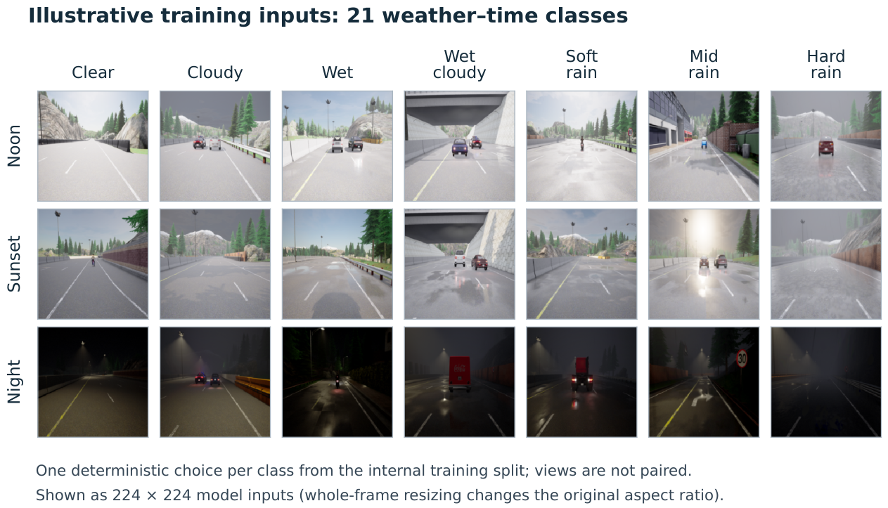
Figure 2.
Recorded training loss and validation macro-F1 for the nine neural runs. Colors identify seeds, and stars mark validation-selected checkpoints. Loss axes are logarithmic, F1 axes begin at 0.80, and lines connect actual epochs without smoothing. The holdout row uses a separate development set.
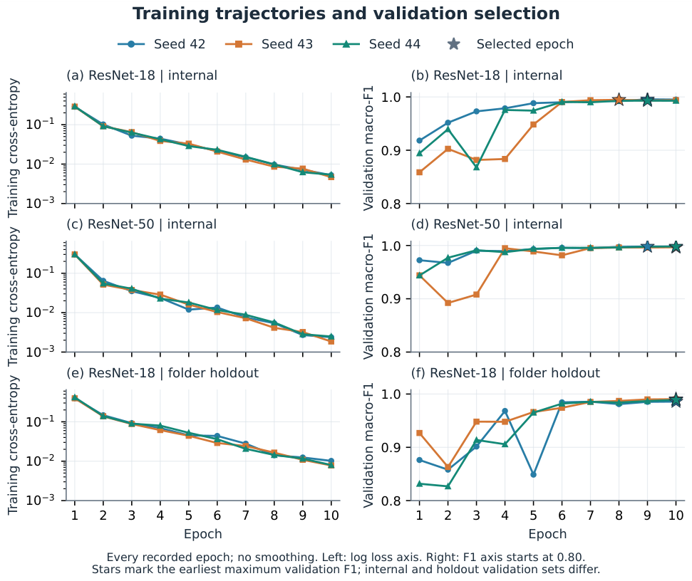
Figure 3.
Classwise F1 and seed-level accuracy. Heatmap cells average three per-run class scores for neural models and retain one fit for each baseline; cells round to two decimals on the same 0–1 color scale. LR, ET, R18, and R50 denote logistic regression, Extra Trees, ResNet-18, and ResNet-50. The accuracy panel distinguishes the internal test () from the original-folder holdout (); its axis is magnified and the populations differ.
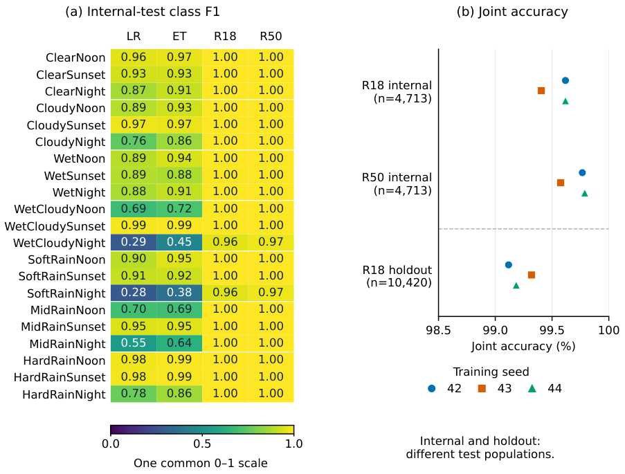
Figure 4.
Paired excess target-logit decrease over ten matched-area random masks. The four areas remove 5, 10, 15, and 25 of 49 cells. Panels separate outcomes and replacement values; lines connect observed means without smoothing. All 210 correct cases and 18 errors remain included.
Figure 4.
Paired excess target-logit decrease over ten matched-area random masks. The four areas remove 5, 10, 15, and 25 of 49 cells. Panels separate outcomes and replacement values; lines connect observed means without smoothing. All 210 correct cases and 18 errors remain included.
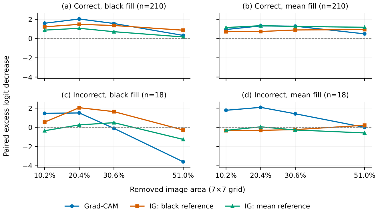
Figure 5.
Casewise black-fill versus mean-fill excess decrease at 10/49 area. The same 228 cases appear in every method panel. Markers distinguish correct predictions and errors; zero lines and the equality diagonal show sign and fill sensitivity.
Figure 5.
Casewise black-fill versus mean-fill excess decrease at 10/49 area. The same 228 cases appear in every method panel. Markers distinguish correct predictions and errors; zero lines and the equality diagonal show sign and fill sensitivity.
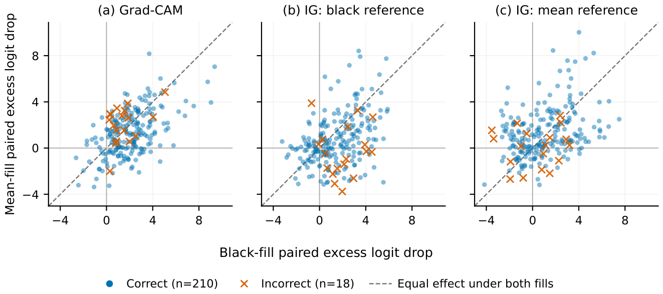
Figure 6.
Fixed illustrative cases 8684 (correct) and 20466 (error), retained from the expanded panel. Both IG references share a full-range symmetric-log scale within each row, linear within 1% of the row maximum absolute attribution; scales vary between rows. Grad-CAM is scaled per case. These examples are illustrative, not representative.
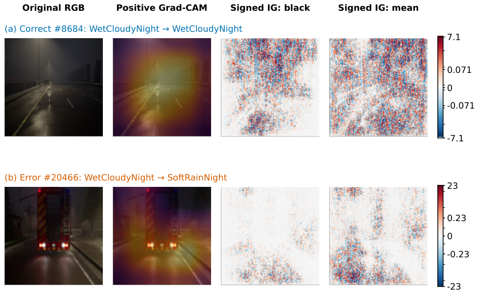
Figure 7.
Trained-versus-randomized Spearman correlations. Heatmaps retain means and defined/total counts; lower panels show individual IG cases and distributions (median, interquartile range, and 1.5-IQR whiskers). Signed pixels, absolute pixels, and positive grids are separate representations. Undefined constant-map correlations remain missing, and numerical failures remain in this full-panel view.
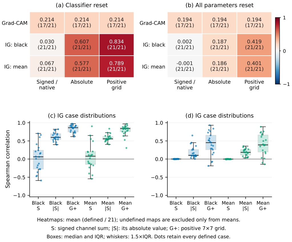
Table 2.
Run-level classification. I and H refer to Table 1. Ep. denotes the validation-selected epoch; P, R, and F1 are joint macro averages. Acc., W, and T are joint, weather, and time-of-day accuracy in percent. Statistical models have no training epoch.
Table 2.
Run-level classification. I and H refer to Table 1. Ep. denotes the validation-selected epoch; P, R, and F1 are joint macro averages. Acc., W, and T are joint, weather, and time-of-day accuracy in percent. Statistical models have no training epoch.
| Model / seed | Split | Ep. | Errors | Acc. | P | R | F1 | W | T |
|---|---|---|---|---|---|---|---|---|---|
| Logistic / 42 | I | – | 866 | 81.63 | 0.810 | 0.816 | 0.810 | 81.75 | 99.77 |
| Extra Trees / 42 | I | – | 698 | 85.19 | 0.848 | 0.852 | 0.848 | 85.25 | 99.89 |
| ResNet-18 / 42 | I | 9 | 18 | 99.62 | 0.996 | 0.996 | 0.996 | 99.62 | 100.00 |
| ResNet-18 / 43 | I | 8 | 28 | 99.41 | 0.994 | 0.994 | 0.994 | 99.41 | 100.00 |
| ResNet-18 / 44 | I | 9 | 18 | 99.62 | 0.996 | 0.996 | 0.996 | 99.62 | 100.00 |
| ResNet-50 / 42 | I | 9 | 11 | 99.77 | 0.998 | 0.998 | 0.998 | 99.79 | 99.98 |
| ResNet-50 / 43 | I | 10 | 20 | 99.58 | 0.996 | 0.996 | 0.996 | 99.58 | 100.00 |
| ResNet-50 / 44 | I | 10 | 10 | 99.79 | 0.998 | 0.998 | 0.998 | 99.79 | 100.00 |
| ResNet-18 / 42 | H | 10 | 92 | 99.12 | 0.991 | 0.991 | 0.991 | 99.12 | 100.00 |
| ResNet-18 / 43 | H | 10 | 71 | 99.32 | 0.993 | 0.993 | 0.993 | 99.32 | 100.00 |
| ResNet-18 / 44 | H | 10 | 85 | 99.18 | 0.992 | 0.992 | 0.992 | 99.18 | 100.00 |
Table 3.
IG numerical completeness and final quadrature-node counts. Absolute-residual summaries include failures. Pass/fail decisions use the endpoint-dependent tolerance in Methods, so a smaller absolute residual need not imply a pass.
Table 3.
IG numerical completeness and final quadrature-node counts. Absolute-residual summaries include failures. Pass/fail decisions use the endpoint-dependent tolerance in Methods, so a smaller absolute residual need not imply a pass.
| Model | Reference | Pass | Fail | Median absolute |
Maximum absolute |
256 | 512 | 1024 |
|---|---|---|---|---|---|---|---|---|
| Trained | Black | 227 | 1 | 0.0221 | 0.114 | 206 | 16 | 6 |
| Trained | Mean | 228 | 0 | 0.0256 | 0.125 | 217 | 11 | 0 |
| Classifier reset | Black | 19 | 2 | 0.00244 | 0.0153 | 7 | 7 | 7 |
| Classifier reset | Mean | 21 | 0 | 0.00332 | 0.0195 | 16 | 4 | 1 |
| Full reset | Black | 21 | 0 | 1.87e-05 | 8.59e-05 | 21 | 0 | 0 |
| Full reset | Mean | 21 | 0 | 3.05e-06 | 1.5e-05 | 21 | 0 | 0 |
Table 4.
All 48 outcome-specific masking settings, grouped into twelve rows. Entries are mean ± sample SD of casewise targeted-minus-random logit decrease, not confidence intervals. IG-black and IG-mean specify attribution references; Fill specifies the replacement value. Areas are 10.20, 20.41, 30.61, and 51.02%.
| Attribution | Fill | Outcome | n | 5/49 | 10/49 | 15/49 | 25/49 |
|---|---|---|---|---|---|---|---|
| Grad-CAM | Black | Correct | 210 | 1.59 ± 1.69 | 2.03 ± 1.94 | 1.57 ± 2.27 | 0.33 ± 2.89 |
| Grad-CAM | Black | Error | 18 | 1.46 ± 1.02 | 1.50 ± 1.30 | -0.10 ± 1.31 | -3.58 ± 1.81 |
| Grad-CAM | Mean | Correct | 210 | 0.94 ± 1.67 | 1.31 ± 1.94 | 1.28 ± 2.04 | 0.49 ± 1.89 |
| Grad-CAM | Mean | Error | 18 | 1.78 ± 1.50 | 2.08 ± 1.58 | 1.41 ± 1.71 | 0.00 ± 2.51 |
| IG-black | Black | Correct | 210 | 1.22 ± 1.67 | 1.48 ± 2.00 | 1.36 ± 1.93 | 0.87 ± 1.72 |
| IG-black | Black | Error | 18 | 0.55 ± 2.26 | 2.04 ± 1.61 | 1.64 ± 1.90 | -0.27 ± 1.81 |
| IG-black | Mean | Correct | 210 | 0.72 ± 1.69 | 0.73 ± 2.16 | 0.89 ± 2.48 | 0.94 ± 2.39 |
| IG-black | Mean | Error | 18 | -0.34 ± 1.88 | -0.31 ± 2.17 | -0.23 ± 2.00 | 0.22 ± 2.03 |
| IG-mean | Black | Correct | 210 | 0.88 ± 1.79 | 1.07 ± 2.28 | 0.71 ± 2.32 | 0.17 ± 2.10 |
| IG-mean | Black | Error | 18 | -0.35 ± 1.83 | 0.26 ± 2.12 | 0.49 ± 2.94 | -1.25 ± 2.25 |
| IG-mean | Mean | Correct | 210 | 1.14 ± 1.97 | 1.33 ± 2.15 | 1.26 ± 2.28 | 1.17 ± 2.02 |
| IG-mean | Mean | Error | 18 | -0.31 ± 1.76 | 0.06 ± 1.69 | -0.27 ± 1.48 | -0.58 ± 2.01 |
Table 5.
Mean randomization correlations for the full panel (F) and common numerical subset (C). n is defined/total; defined counts agree for signed/native and positive-grid representations within each row. For Grad-CAM, native and positive-grid maps coincide. Full-panel absolute-map results are shown in Figure 7.
| Reset | Attribution | n F | n C | Signed F | Signed C | Grid F | Grid C |
|---|---|---|---|---|---|---|---|
| Classifier | Grad-CAM | 17/21 | 15/19 | 0.214 | 0.165 | 0.214 | 0.165 |
| Classifier | IG-black | 21/21 | 19/19 | 0.030 | 0.049 | 0.834 | 0.843 |
| Classifier | IG-mean | 21/21 | 19/19 | 0.067 | 0.088 | 0.789 | 0.781 |
| Full | Grad-CAM | 17/21 | 16/19 | 0.194 | 0.154 | 0.194 | 0.154 |
| Full | IG-black | 21/21 | 19/19 | 0.002 | 0.002 | 0.419 | 0.442 |
| Full | IG-mean | 21/21 | 19/19 | -0.001 | -0.000 | 0.401 | 0.387 |
Disclaimer/Publisher’s Note: The statements, opinions and data contained in all publications are solely those of the individual author(s) and contributor(s) and not of MDPI and/or the editor(s). MDPI and/or the editor(s) disclaim responsibility for any injury to people or property resulting from any ideas, methods, instructions or products referred to in the content. |
© 2026 by the authors. Licensee MDPI, Basel, Switzerland. This article is an open access article distributed under the terms and conditions of the Creative Commons Attribution (CC BY) license (http://creativecommons.org/licenses/by/4.0/).
Copyright: This open access article is published under a Creative Commons CC BY 4.0 license, which permit the free download, distribution, and reuse, provided that the author and preprint are cited in any reuse.