

Submitted:
05 October 2026
Posted:
08 October 2026
You are already at the latest version
Abstract
Statistical analysis usually begins from recorded values treated as draws from a distribution. Those values acquired their numerical form through processes—choice of unit, rounding and coding, biological, arithmetic and institutional constraints, composition from other quantities, aggregation and ordering—that the abstraction X1, . . . , Xn ∼ F leaves implicit. This article develops a construction-aware identification framework for recorded numerical data. An upstream state Z passes through a construction map indexed by a regime M to give the recorded value X, which an analyst transforms into a representation P(X) on which a diagnostic is computed. The framework makes the construction regime an explicit inferential target alongside the upstream state and shows that the two identification problems can move in opposite directions: a rounding rule can be ignorable for inference about a mean and yet identifiable from terminal digits. It places the analyst’s representation on the same chain as the recording process, so that a distinction the recorded values carry can be destroyed before any diagnostic is computed. Formal results characterize when construction regimes are observationally distinguishable from recorded values, when support alone can exclude a regime, and when a representation preserves or destroys that distinction. A locating vocabulary—unitization, quantization, constraint, composition, aggregation—says where numerical structure entered a record, and worked cases from temperature archives, survey blood pressure, the genetic code, check digits, marathon qualifying standards, seawater sound speed, tide gauges and federal spending records show the framework operating in each class. The practical consequence is a change in what a numerical diagnostic reports: not an anomaly flag, but whether the construction regime is identified, partially identified, excluded, or not identified by the information at hand.
Keywords:
coarse data
; data provenance
; identification
; measurement
; observational equivalence
; representation
1. Constructed, Not Sampled
Pick up a numerical column—prices, ages, blood pressures, transaction amounts, temperatures —and the natural statistical abstraction is . The abstraction is useful and usually harmless. It also suppresses a question that is logically prior to it: how did the values acquire the numerical form in which they entered F?
The title of this article could be misread as a denial that recorded data can be a sample. It is not. Sampling and construction answer different questions. Sampling describes how observational units enter a data set: which households were interviewed, which transactions were retained, which stations reported. Construction describes how the values attached to those units acquired numerical form: in what unit they were written, to what resolution they were rounded, which coding rules and institutional limits they had to satisfy, whether they were computed from other quantities, and how they were summed or sequenced. A data set can be both sampled and constructed, and most are. The U.S. National Health and Nutrition Examination Survey selects its participants by a carefully documented probability design; the blood pressures it records for those participants are, in addition, the output of a measurement and recording protocol. A statement about the first is not a statement about the second.
Construction in this sense is ordinary, not pathological. A reading taken from a mercury column by a trained examiner, an amount entered to the cent under a spending authority, an age reported in completed years, a temperature archived in tenths of a degree after conversion from another scale, a line total computed as unit price times quantity: each is the product of a process that is usually well designed and often essential to the comparability of the values. Construction is also not a synonym for measurement error. There need be no pristine numerical truth beneath a recorded value against which its construction counts as contamination; the philosophy of measurement has argued at length that units, fixed points, and instruments are how a quantity becomes measurable in the first place (Chang 2004,Tal 2013). Nothing below depends on taking a side in that literature. It depends only on recognizing that a recorded value is the output of a process, and that the process has structure a statistician can describe.
That structure has a precise statistical consequence. Suppose a quantity Z with distribution enters a construction process, and the recorded value is . Then the recorded values certainly have a distribution, and it is the pushforward
the distribution obtained by passing the upstream quantity through the recording process. So “constructed, not sampled” does not mean that fail to be a statistical sample. It means that treating as primitive hides the fact that it is jointly determined by two things—the upstream variation in and the map H—and that different combinations of the two can produce the same , or distributions that differ in ways that are informative about the map rather than about the quantity.
This matters most when an analyst reads a pattern in recorded values as evidence about how they were produced. A leading-digit screen is read as evidence about how amounts were generated; a terminal-digit or heaping index as evidence about how ages or blood pressures were recorded; a reconstruction error or isolation score as evidence that something in a record’s production was irregular. Each of these readings passes through two maps, not one. The first is the construction map, which determines what information about the upstream state, and about the process itself, survives into the recorded value. The second is the representation the analyst chooses—leading digits, terminal digits, ranks, an embedding, a histogram—which determines what information about the recorded value survives into the diagnostic.
Statistical practice has powerful theories for sampling, measurement error, coarsening, latent variables, sufficiency, anomaly detection and representation. What it lacks is a common inferential language for a different question: what, if anything, do recorded numerical values identify about the process that gave them their numerical form? Each of those theories answers a piece of the question under its own assumptions. Taken separately, they do not generally provide a common inferential framework that places the construction map and the analyst’s representation on one chain and asks, at each link, what remains identified; multimedia forensics comes closest, for images (Section 5.2). This article supplies that language for recorded numerical data.
The distinction at its center is not a renaming of a nuisance parameter. A rounding rule can be ignorable for inference about a mean—coarsening at random in the sense of Heitjan and Rubin (1991)—and yet identifiable from the terminal digits of the recorded values. What the data reveal about the state and what they reveal about the regime are different questions, and they can have opposite answers.
This article develops a construction-aware identification framework for recorded numerical data and makes four contributions. First, it makes the construction regime an explicit inferential target, distinct from the upstream state, and shows that the two identification problems can move in opposite directions: construction can destroy information about the state while imprinting restrictions that identify the regime among a set of candidates (Section 2 and Section 3). Second, it places the analyst’s representation on the same inferential chain as the recording process and makes representation-induced nonidentification exact: no diagnostic computed from can separate what P has merged, however much the recorded values carry (Section 4). That gives a precise statistical meaning to the phrase geometry is not meaning. Third, it introduces a domain-independent locating vocabulary—unitization (U), quantization (Q), constraint (C), composition (G), and aggregation and sequencing (A)—that says where a numerical feature entered a record and therefore what evidence could identify the process that put it there. Fourth, it turns these ideas into an operational workflow that replaces an undifferentiated anomaly flag with an identification statement about the construction regime: identified, partially identified, excluded, or not identified given the available information (Section 7). The constituent tools—pushforwards, structural zeros, sufficiency, the data-processing inequality—are classical and are credited as such; the framework built from them, and what it changes about how claims concerning construction are made and reported, is the contribution.
Section 6 demonstrates the framework on real data in every construction class: temperature archives (U), blood pressure in a national survey (Q), the genetic code, check digits and marathon qualifying standards (C), seawater sound speed (G), and tide gauges (A). It ends with a federal spending column in which the framework’s correct output is that the regime is not identified.
The payoff for the reader is concrete. A statistician who adopts the framework can take a numerical diagnostic—a digit law, a heaping index, an anomaly score, a threshold screen, a marginal histogram, a periodogram—and state what construction claim it can support, which distinctions its representation has already erased, what additional information would identify the regime, and when the correct conclusion is that the process is not identified. The question is not confined to anomaly detection. Wherever recorded values are pooled across instruments, protocols, units or eras, whether a numerical pattern is evidence about the data or about their making is a question the analyst has to answer, and the framework says how.
The rest of the article proceeds as follows. Section 2 sets out the chain and the two inverse problems. Section 3 establishes what survives construction, including when support alone excludes a regime. Section 4 treats the representation as a second information bottleneck. Section 5 places the framework among the statistical literatures that address parts of it. Section 6 runs it across U, Q, C, G and A in real data, Section 7 turns it into seven questions an analyst can ask of any numerical diagnostic, and Section 8 draws the consequences.
The question that governs everything that follows is this:
What can recorded numerical data identify about the quantities, and about the construction regimes, that produced them, and what further information is lost when those data are transformed into the representation a statistical diagnostic uses?
2. Construction Maps and Two Identification Problems
2.1. The Chain
Figure 1 shows the chain. It has five objects and four maps,
and each needs a careful definition, because most confusion in this area comes from attaching a conclusion to the wrong one.
The upstream state Z
Z is whatever enters the construction operation under study. It is not “the true value.” Its status is relative: it is upstream of the particular operation being analyzed, and it may itself be the output of earlier measurement or construction. Before a rounding step, Z is the unrounded number; before a unit conversion, it is the value on the source scale; before a composition, it may be a vector such as a unit price and a quantity; before an aggregation, a sequence of component transactions. Defining Z relative to an operation sidesteps the question of whether there is a numerical truth at the bottom of the chain.
The construction regime M and the construction map
M indexes the process by which a recorded value acquired its numerical form, and is the corresponding map. In the simplest case is a deterministic function, . In general it is a Markov kernel,
which covers stochastic instruments, measurement error, coding mistakes, and any recording step that does not return the same output for the same input. Deterministic maps are the special case . Nothing below requires more than this: the kernel is there so that “construction” does not silently mean “deterministic rounding.”
A construction map is usually a composition of simpler operations, , and it is convenient to have names for the kinds of operation that recur. Five suffice for most applications: unitization (U), the choice of unit and scale; quantization (Q), integerization, rounding, truncation, and categorical coding; constraint (C), arithmetic or institutional rules a value must satisfy, such as a cap, a threshold, or a check digit; composition (G), a value computed from other quantities, such as price times quantity or a derived index; and aggregation and sequencing (A), summation over components and the order in which records are written. These are a locating vocabulary, not a theory and not a fixed order. Composition can precede final quantization or follow it, an aggregation can precede a coding rule, and any family can be absent. Their use is to say where in a construction process a given feature of the recorded data was made, and therefore which evidence can and cannot reach it.
The recorded value X
X is what appears in the data set. One feature of recorded values is worth stating at the outset because it is used repeatedly: a recorded number is a finite numeral, so the set of values a recording system can write is countable. However continuous Z may be, a finitely represented X takes values in a countable set, and its distribution can be described by a probability mass function.
The representation P
A statistical method rarely uses all of X. It uses leading digits, terminal digits, magnitudes, ranks, residuals from a fitted model, Fourier coefficients, an empirical histogram, a learned embedding, or a vector of engineered features. Write the representation as a measurable map and . Where a method uses many records at once—a histogram, a serial correlation, a periodogram—P acts on the whole record rather than on each value separately, and the distinction matters (Section 2.2).
The baseline B and the diagnostic D
The baseline is whatever makes a diagnostic comparative: a reference distribution such as a digit law, a null model, a training sample, an empirical neighborhood, a fitted reconstruction model, or a threshold. The diagnostic is the score, flag, conformity statistic, or test statistic. It is the only part of the chain a reader of an analysis usually sees.
The claim
An analyst who moves from a value of S to the statement “this pattern indicates mechanism m” has made a claim about M that has traversed every map in (2). It is a claim about a specific regime, read through a specific representation, against a specific baseline. We refer to this triple as a mechanism–projection–baseline claim, in which the mechanism is the construction regime M. The rest of the article asks what each link of the chain contributes to whether such a claim can be true.
2.2. Heterogeneous Regimes
Recorded columns are rarely produced by one regime. A station archive may be written under one convention before an instrument change and another after; a ledger may combine manually entered and system-computed amounts; a survey may combine two measurement protocols. Write for the regime under which record i was produced. When the records are exchangeable and the regimes take finitely many values with shares , the marginal distribution of a recorded value is the mixture
Two features of (4) belong to the framework from the start rather than to a later caveat. First, the upstream law is indexed by the regime: , not . Regimes and states can be dependent. An instrument change can coincide with a change in climate; a new recording system can arrive with a new population of transactions. Whenever that happens, a change in across regimes confounds a change in the construction map with a change in what was being constructed, and any argument that reads the change as evidence about M has to separate the two.
Second, (4) is a statement about the marginal law of a single recorded value, and it therefore represents heterogeneity only for diagnostics that are functions of the marginal: digit laws, heaping indices, magnitude scores, anything computable from the pooled histogram. Diagnostics that use order, serial dependence, composition across fields, or aggregation are functionals of the joint law of the record , which the marginal does not determine. Two records can share an empirical distribution exactly and differ arbitrarily in their dependence: a tide-gauge series and a random permutation of it have the same histogram, and only one carries the semidiurnal signal (Section 6.5). When the regime acts on order—batching, sorting, carrying forward a previous value—the object of inference is the joint law, and the mixture of marginals is the wrong model. In what follows, X may denote a single value or a whole record; the results hold for either, provided the law in question is the law of whatever the diagnostic actually reads.
2.3. Two Inverse Problems
The chain (2) begins with a forward map from Z to X. There are two inverse questions one can ask of it, and they are different:
State identification asks what the recorded data reveal about the upstream quantity or its distribution: given that values were rounded, heaped, top-coded, or converted, what can be said about or about a particular z? Regime identification asks what the recorded data reveal about the process that gave them their form: were these values rounded to even, entered by hand, converted from another unit, computed rather than measured, written under one protocol or two?
To make the second precise, let be a set of candidate regimes and, for each m, let be the set of upstream laws the analyst is prepared to entertain under that regime. The model is the set of pairs with , and each pair induces a law for the recorded value,
The regime is identified if implies , for all admissible . That is the classical definition of identification (Koopmans Reiersøl 1950,Rothenberg 1971) applied to the construction regime, with the upstream law playing the role of a nuisance parameter. Two parameter pairs and are observationally equivalent if . When some admissible pair under is observationally equivalent to some admissible pair under , the two regimes are not separated over the admissible classes: for those upstream laws, no record distinguishes them. Between these extremes lies partial identification: the data narrow the set of regimes without reducing it to a point (Manski 2003,Tamer 2010).
The key observation is that the two inverse problems need not move together. A construction map can be very lossy for Z and very informative about M, or the reverse. Rounding to the nearest even integer discards more information about Z than rounding to the nearest integer, yet a single odd value proves that the coarser rule was not the one applied. Conversely, let record Z and record for a known offset c. Given the regime, each map is lossless for Z; yet if the admissible upstream laws form a location family, each pair is observationally equivalent to , where is F shifted by , so the two regimes are not separated and no record distinguishes them. Classical identification and coarse-data work has developed the first question extensively, often treating the recording process as a nuisance standing between the analyst and Z. The second question is the one a numerical diagnostic answers when it is read as evidence about how the numbers were produced; such diagnostics often answer it without placing the claim on the same identification-and-representation chain, and it is governed by different considerations.
3. What Survives Construction
This section establishes the two boundaries of regime identification from recorded values. The negative boundary is observational equivalence: where candidate regimes induce the same law for what the analysis observes, no statistic separates them. The positive boundary is support exclusion: where a regime cannot produce a value, one observation of that value rules it out, without specifying the upstream law within the admissible class. The proofs are short; the content lies in what is being identified and relative to what information.
3.1. Observational Equivalence
Proposition 1
(Observational equivalence). Let and be two admissible pairs that induce the same law for the observable, . Then for every measurable statistic T of the observable, the law of T is the same under both pairs, and every test of against based on the observable has power equal to its size.
Proof.
Measurable maps preserve equality of laws: if then for every measurable A. A test therefore has the same rejection probability under both pairs. □
The proposition’s force lies in what “the observable” is taken to be. It applies to whatever the analysis actually conditions on: a single value, an i.i.d. sample (the product law ), a whole ordered record, or a record together with auxiliary fields. That is what makes it a statement about an information set rather than about the regimes themselves. If and are observationally equivalent given X, they may not be given , where W is a metadata field, a label on a subset of records, a repeated measurement of the same unit, the same records under an intervention, or a documented standard. Adding W replaces the law of X by the joint law of , and the proposition must be checked again.
This blocks two opposite overreadings. One is pessimistic: the proposition does not say that construction regimes cannot be distinguished scientifically. It says that this information set does not distinguish these pairs. The limit is evidential, and the remedy for it is to change the information available, not to compute a more elaborate statistic on the same information. The other overreading is optimistic: a diagnostic that “detects” a regime under one admissible upstream law may detect nothing under another. Because F enters (6) as a nuisance, observational equivalence is a property of the model, meaning the pair of candidate regimes together with the range of upstream laws the analyst is willing to admit. Rounding to the nearest integer and rounding to the nearest even integer are distinguishable if every admissible upstream law puts positive mass within of some odd integer, and not separated over the admissible class if an admissible law may be concentrated within of the even integers—which a law with a density can be. The analyst’s assumptions about F are part of every regime-identification claim, whether stated or not.
3.2. Support Exclusion
The positive counterpart is that construction can leave marks that are not merely different in frequency but different in possibility. Because recorded values are finite numerals, each law is a probability mass function on the countable set . Everything in this subsection is conditional on the maintained candidate family and the admissible upstream classes : an exclusion does not require specifying which distribution within generated the data, but it does depend on what admits. Define the attainable set of regime m as the set of values it can produce under some admissible upstream law,
where ; and, for an observed record in which every value is assumed to come from the same regime, the support identification set
Proposition 2
(Support exclusion). Assume the model of Section 2.3, with countable, and suppose that the true regime belongs to , that every record in was produced by it, and that the true upstream law is admissible for it. Then:
- (a)
- if , then observing x excludes regime m: under every admissible the probability of observing x is zero;
- (b)
- the true regime belongs to with probability one, whatever admissible upstream law generated the data;
- (c)
- if and , a single recorded value identifies which of the two produced it, without error.
Proof. (a) If then for every admissible F by (7). (b) Under the true pair , for each i, and a countable union of null events is null; since , every lies in almost surely. (c) follows from (a) and (b). □
Proposition 2 gives the framework a three-way vocabulary for regime identification from support alone: the set may be a single regime (point identification), a proper subset of the candidates (partial identification), or all of them (no exclusion). Every one of these conclusions is relative to the candidate set: a support signature excludes candidates, and it identifies a regime only among the candidates entertained, since a regime outside may produce the same values. When records may come from different regimes (Section 2.2), the single-regime set is replaced by a statement about sets of regimes: the record is compatible with a set of regimes, each record produced by one of them, exactly when every (Lemma A1, Appendix A.1). An empty is then evidence of heterogeneity, or of a regime outside the candidate set, rather than a contradiction. Three further properties of the identification set are worth noting, because they are what make it useful in practice and what limit it.
First, it does not require specifying the upstream law within the admissible class. The attainable set is a union over every admissible F, so an exclusion does not depend on which admissible upstream distribution generated the data, and in particular it is unaffected by the regime–state confounding of Section 2.2 provided each lies in . A change in can move frequencies anywhere within ; it cannot put mass outside it.
Second, it is exact in finite samples but not sharp. A single value outside excludes m with certainty; by contrast, when candidate regimes share support and differ only in probabilities within it, finite-sample discrimination is necessarily probabilistic. But uses only which values occurred, not how often. When attainable sets are nested—the even integers are a subset of the integers—the larger regime can never be excluded by support, and distinguishing it from the smaller one requires frequency information and therefore more specific assumptions about F. If the records are i.i.d. with law Q and is finite, then as n grows is eventually equal to with probability one. The sharp identified set, , can be strictly smaller, and computing it uses the full content of the admissible classes , not only their attainable sets (Appendix A.2).
Third, the exclusions are exactly as strong as the construction model that defines . If the kernel has full support—if every value in can occur under m through measurement noise, keying errors, or occasional departures from protocol—then and no exclusion is possible. Structural zeros—cells that are empty by construction rather than by chance, in the sense long used for contingency tables (Bishop et al. 2007)—then become near-zeros, and support exclusion becomes a likelihood contrast: values that are rare under m and common under shift evidence between the two without settling it. The construction model’s account of what cannot happen is a modeling assumption like any other, and Proposition 2 inherits it.
Example 1
(Three rounding regimes). Let Z have a continuous distribution on the positive reals, and consider three candidate regimes that record it as an integer: rounds to the nearest integer, to the nearest even integer, and to the nearest multiple of five, with halves rounded up. With all continuous upstream laws admissible, the attainable sets are , and (Figure 2). An observed 7 gives : among the three candidates, the regime is point-identified from one value. An observed 4 gives , and an observed 10 gives all three. A record also leaves all three; adding a 14 removes , and adding a 13 removes both coarse regimes.
The state and regime problems need not move together. Under the recorded value 10 locates Z only in ; under , in . The coarsest regime is the least informative about the state, yet a single recorded value that is not a multiple of five excludes it. Nesting limits what support can do: contains the others, so is never excluded by support, and an all-even record is compatible with both and . Distinguishing them requires the frequency of even values, and that requires an assumption about F: if Z has a density that is roughly flat over intervals of length two, an i.i.d. all-even record of length n has probability about under ; if Z may be concentrated near even integers, the corresponding pairs are observationally equivalent and the two regimes are not separated. Support exclusion does not require specifying the frequency distribution within the admissible upstream class; frequency identification does. Finally, if the recording of is occasionally mistyped by one unit, its attainable set becomes all integers and an odd value becomes evidence against in proportion to the error rate rather than proof. Real heaping, as in reported ages, is of that kind, and its analysis is a mixture problem rather than a support problem (Heitjan Rubin 1990).
Where the positive result comes from
The two propositions together locate the source of regime information. A construction map that sends every upstream law into the same attainable set and the same family of mass functions as its competitor leaves nothing to identify, whatever the sample size. A map that restricts the attainable set—to a grid, to a residue class, to values that satisfy an arithmetic rule—imprints a signature that can be read without specifying an upstream distribution within the admissible class. That is the sense in which construction is not only a source of information loss. The same rounding step that coarsens what can be known about Z can make the regime that performed it identifiable, among the candidate regimes, from a handful of values. Specific construction families can make such restrictions explicit; here the point is only that the possibility follows generally from treating the recorded value as the output of a construction map.
4. Representation Is a Second Bottleneck
Construction determines what the recorded value X carries. The analyst then chooses P, and P determines what of X the diagnostic will ever see. The two maps answer different questions: asks what the recording process preserved; asks what the analyst subsequently retained. A distinction can survive the first and be destroyed by the second, and when that happens no sophistication downstream of P can restore it.
4.1. A Bound on What a Representation Can Separate
Let denote total variation distance, and for a representation P write for the law of when .
Proposition 3
(Representation bound). Let and , and let P be any measurable representation. For every test that sees only ,
and the first inequality is attained. The second inequality is an equality when P is sufficient for . In particular, if , no diagnostic computed from has power exceeding its size, whatever the information in X.
Proof.
For with values in , the left side equals
with equality when is the indicator of the set on which has the larger density. For the second inequality,
is a supremum over the sets of the form , a subclass of all measurable sets. If P is sufficient for , the likelihood ratio is a function of P by the factorization theorem, so the maximizing set for is of the form and the two suprema coincide. □
The bound says three things. The best any diagnostic on can do, in the sense of power minus size for distinguishing two fully specified alternatives, is the total variation distance between their pushforwards through P. That distance can only shrink as information is discarded: this is the data-processing inequality, and in the language of the comparison of experiments it says that a representation is a garbling of the recorded data and can never be more informative than they are (Blackwell 1953,Le Cam 1964). And a representation that is sufficient for the two fully specified laws loses nothing for distinguishing them—not for this test only but for any test, loss, or prior—which is a different and much weaker requirement than being sufficient for everything about X. Preserving the total variation distance alone asks even less: only that P never merge a value at which exceeds with one at which exceeds (Lemma A3, Appendix A.3). Proposition 1 is the special case in which the right-hand side of (9) is zero with P the identity. A representation can discard most of X and still be ideal for a particular pair of laws, if what it keeps is the part on which they differ. Two regimes, however, are composite: each is indexed by its admissible upstream laws. A representation preserves the contrast between two regimes only if it preserves discrimination between and uniformly over the admissible nuisance laws, and sufficiency for one fully specified pair does not guarantee that.
For the analyst, the practical form is a corollary about invariance. Many representations are invariant to some transformation of the record: an unordered digit histogram does not change when two digits are swapped; an empirical distribution does not change when records are permuted; a leading-digit summary does not change when a value is multiplied by a power of ten.
Corollary 1
(Invariance). Let G be a set of measurable transformations of the record space with for every . If regime acts on the output of regime by applying a transformation from G—that is, is the law of with , where the transformation may be random and may depend on X (Appendix A.4)—then , and no diagnostic on distinguishes from . In a balanced paired design over pairs , every score that depends on the record only through P assigns the two members of each pair the same value, so the scores of the two classes form identical multisets and the area under the ROC curve is exactly .
Proof.
for every realization, so the two laws of coincide. In the paired design the two classes carry identical multisets of scores, and the area under the ROC curve of two identical score distributions, with ties counted as one half, is . □
The corollary is worth stating separately because its hypothesis can be checked without data. Whether a representation is blind to a regime contrast is often settled by asking whether the regime acts by a transformation the representation is invariant to. If it does, the representation is blind by construction, not merely weak in practice, and that fact is fixed before any model is fit.
4.2. Geometry Is Not Meaning
Generic anomaly detectors make the point vivid. An isolation forest, an autoencoder’s reconstruction error, or a robust low-rank residual (Candes et al. 2011,Liu et al. 2008,Ruff et al. 2021) answers a well-posed question: which records are isolated, or poorly reconstructed, in the geometry that P defines? That question is not the same as which regime produced which records. A high score says that a record sits in a sparse region of relative to the baseline; it carries a mechanism label only to the extent that the regimes of interest are separated in , which is exactly what Proposition 3 measures. Geometry is not meaning. A detector can be excellent at the geometric question and uninformative about the mechanistic one, and the difference is a property of P and the regime pair, not of the detector’s sophistication.
The same holds for learned representations. That latent factors of variation are not identifiable from the distribution of the data without inductive biases or supervision is a central result of the disentanglement literature (Locatello et al. 2019,Schölkopf et al. 2021). In the present terms, a representation learned to compress or reconstruct X retains what its training objective rewards, and there is no reason for that to coincide with what distinguishes a given pair of regimes. Probing a learned representation for a property presupposes an external criterion it was not trained on (Alain Bengio 2016,Belinkov 2022). No learner that sees only can recover a distinction P has removed; a different representation, or different information, can.
4.3. Mechanism, Projection, Baseline
Proposition 3 explains why a mechanism claim made from a diagnostic has three parts. When an analyst reads as evidence for regime m, the claim depends on the regime contrast it is about (which m, against which alternatives), on the representation (whether the contrast survives P), and on the baseline (what B treats as ordinary). Leave the regime implicit, and the claim cannot be checked against Proposition 3 at all, because the bound is defined only for a specified pair of laws. Leave the baseline implicit, and a score can change its meaning when the baseline’s domain changes: a leading-digit law is a reference only under conditions on the upstream law (Hill 1995), and where those conditions fail a deviation from it cannot be attributed specifically to M: the upstream law, the construction regime, or both may account for it.
The triple is therefore not an additional framework but a reporting convention that follows from the chain. A diagnostic may legitimately describe geometry and stop. Once it is read as evidence about the construction process, it should say which regime contrast it is about, why that contrast survives the representation, and what the baseline assumes about the upstream law.
5. Statistical Literatures That Solve Pieces of the Problem
The framework of Section 2, Section 3 and Section 4 brings together statistical ideas that have developed in several mature literatures, but it places them around a different inferential object. Coarse-data and measurement-error methods primarily ask what recorded data reveal about an upstream state; latent-regime methods infer unobserved components under structural assumptions; sufficiency and representation theory ask what a map retains; numerical diagnostics score projected geometry against a baseline. Each divides the chain (2) differently, holding some links fixed and treating others as the object of inference. Comparing those divisions shows what the framework adds: it puts the construction regime and the analyst’s representation on one chain and asks what is identified at each map, and read that way the literatures become complementary pieces of a single construction-aware identification problem. This section organizes them by the question they answer rather than by field, and Table 1 summarizes the result.
5.1. When the Construction Map Is a Nuisance and the State Is the Target
The oldest statistical treatments of construction are about rounding and grouping. Sheppard’s corrections adjust the moments of a grouped distribution for the width of its cells (Sheppard 1897), and the problem of inference from rounded or grouped continuous data has been reviewed in Statistical Science (Heitjan 1989); Dempster Rubin (1983) analyze when rounding error in regression can be ignored. The general theory is that of coarse data. Heitjan Rubin (1991) define data as coarsened when one observes a set known to contain the exact value rather than the value itself, and give conditions—coarsening at random—under which the coarsening mechanism can be ignored in likelihood or Bayesian inference about the underlying quantity, extending the missing-data framework of Rubin (1976), in which missingness is the extreme case of coarsening (Jacobsen Keiding 1995,Little Rubin 2019). Measurement-error models play the same role for noisy rather than coarsened recording (Carroll et al. 2006,Fuller 1987), and the econometric literature on nonclassical error has made the identification question explicit, showing in particular how auxiliary information such as instruments or repeated measurements restores identification that the error alone destroys (Hu Schennach 2008,Schennach 2016). Interval-recorded outcomes and regressors lead naturally to partial rather than point identification of the underlying quantity (Manski Tamer 2002).
In the terms of this article, these literatures study state identification, , given a construction map that is known or modeled. They do not ignore the regime. Results on nonclassical measurement error identify the error distribution—the kernel —jointly with the distribution of the latent quantity, using instruments or repeated measurements (Hu Schennach 2008,Schennach 2016), and that is regime identification, carried out because the regime is a nuisance whose law must be known before Z can be recovered. The coarse-data strand asks the complementary question of when the regime can be left out of the analysis altogether. That is where the present framework departs from it, and the departure is complementary rather than critical. Ignorability is a statement about inference on Z: it says that the construction mechanism carries no information about Z beyond what the recorded values already convey. It is not a statement that the recorded values carry no information about the mechanism; as noted in Section 1, a rounding rule can be ignorable for estimating a mean and identifiable from the terminal digits. The two inverse problems of Section 2.3 separate exactly at this point.
5.2. When the Regime Is Latent
A second group of literatures treats the regime itself as unobserved and infers it. The closest statistical precedent for the construction map is the modeling of heaping. Heitjan Rubin (1990) treat reported ages as the output of a latent rounding behavior applied to exact age, and Wang Heitjan (2008) model a self-reported cigarette count as a deterministic function of a precise underlying count and a heaping-behavior variable, both partially observed, with inference on the two jointly. Related models treat heaping in durations (Torelli Trivellato 1993), asymmetric rounding in density estimation (Gro Rendtel 2016), and experimental evidence on why respondents round (Ruud et al. 2014). These are exactly models of the form with M latent and unit-specific. In climate science, Rhines et al. (2015) recover the most likely original precision and units of individual temperature observations with a hidden Markov model over recorded values, and X. Zhang et al. (2009) show how recording precision alone can bias derived climate indices. Outside statistics, multimedia forensics infers how an observed object was produced, and its formal treatment anticipates several ingredients of the present chain. Component forensics estimates the algorithms and parameters inside a camera’s processing modules from its output images alone (Swaminathan et al. 2007). Kirchner (2012) defines image forensics as the reconstruction of an image’s generation process and the forensic task as assigning an image of unknown provenance to a known class of generation processes; he notes that later processing can wipe out the traces of earlier stages and that side information changes what can be inferred, and he defines a feature representation as a projection of the image into a feature space, with class distributions induced there. Böhme Kirchner (2013) treat forensic inference and counter-forensics as a decision problem over composed generation processes. These ideas do not originate here. What the present article adds is a statistical formulation across domains: state versus regime identification under a nuisance class of upstream laws, support versus frequency evidence, the representation as an explicit second information bottleneck, and a workflow for ordinary numerical diagnostics.
More generally, recovering latent regimes is the business of finite mixtures, latent-class and hidden Markov models, and change-point analysis. Identifiability of mixtures requires structure (Frühwirth-Schnatter 2006,McLachlan Peel 2000,Teicher 1963); for latent-class and related models it holds generically under conditions on the number of observed variables (Allman et al. 2009); regime-switching and change-point methods locate changes in a data-generating process over time (Aminikhanghahi Cook 2017,Hamilton 1989,Truong et al. 2020). Behind all of these lies the general theory of identification, from the classical definitions of observational equivalence (Koopmans 1949,Koopmans Reiersøl 1950,Rothenberg 1971) to partial identification, in which the data and maintained assumptions determine a set rather than a point (Imbens Manski 2004,Manski 1989,Manski 2003,Molinari 2020,Tamer 2010); Lewbel (2019) surveys the many senses in which the word is now used. Bounds that follow from a bounded outcome support are among the earliest results of partial identification (Manski 1989), and the support identification set of Section 3.2 is loosely analogous: it, too, draws a set-valued conclusion from what values are possible rather than from how often they occur.
The present framework borrows its definitions from this literature. What differs is the status of the regime. In measurement-error and heaping models the regime is usually a nuisance, or a latent component estimated in order to recover Z; here it is a discrete, interpretable object that a diagnostic reports on. Three consequences follow. Regimes are described by the kinds of operation they consist of (the U/Q/C/G/A vocabulary of Section 2.1, which Section 6 puts to work on real data), so the restrictions they can imprint can be read off the construction. Support and frequency are distinguished as sources of regime information (Section 3.2): support restrictions can exclude candidate regimes without specifying an upstream distribution within the maintained admissible class, while frequency restrictions, which mixture-based regime inference typically uses, rest partly on more specific assumptions about . And the analyst’s representation is treated as a second map with its own identification limits, which these literatures, working with the recorded values themselves, do not need to consider.
5.3. When the Data-Production Process Is the Subject
Survey methodology has the most developed account of data production. The total survey error framework decomposes error into a representation side—coverage, sampling, and nonresponse, which determine which units are observed—and a measurement side, which determines what is recorded about them (Biemer 2010,Groves Lyberg 2010). This is close to the distinction between sampling and construction drawn in Section 1; the measurement side includes processing error from coding and editing, which is construction carried out after collection, and edit rules that force records to satisfy arithmetic and logical constraints are constraint operations in exactly the sense of Section 2.1 (Fellegi Holt 1976). Mixed-mode surveys show the regime–state dependence of Section 2.2 in practice: when the mode of data collection affects both who responds and what they report, selection and measurement effects are confounded (Jäckle et al. 2010). It should be noted that the word “representation” means something different there, namely how units represent a population, from its meaning in Section 4, where it is the analyst’s feature map. The growth of administrative, transactional, and other organic data has sharpened the point, because for such data the measurement side is set by systems built for other purposes (Groves 2011,Hand 2018,Japec et al. 2015,L.-C. Zhang 2012). Meng (2018) shows how a small defect in the inclusion mechanism can dominate the error of a very large data set; the analogous question for construction is how a recording convention shared by many records shapes what they can reveal. Statistical disclosure limitation is construction applied deliberately: a differentially private release is an explicitly stochastic construction kernel, and its publication raises both inverse problems at once, since users must infer the confidential values through a mechanism whose design is, by policy, public (Gong 2022,Reiter 2019).
Measurement theory supplies the conceptual background. Statistics has long engaged the representational theory of measurement (Hand 1996,Hand 2004,Krantz et al. 1971,Stevens 1946), and recent philosophy of measurement treats the outcome of a measurement as characterized through a model of the measurement process rather than independently of it (Mari et al. 2021,Tal 2013), a view anticipated by historical work on how scales were constructed (Chang 2004). Philosophy of data makes the corresponding point about records: data are made, curated, and moved, and what they can serve as evidence for depends on that history (Leonelli 2016,Leonelli 2019). Psychometrics asks the regime question across groups under the name of measurement invariance: whether an instrument relates observed scores to the latent trait in the same way in each group, which is a question about whether the construction kernel differs between groups (Meredith 1993). Practical counterparts include documentation standards for data sets (Gebru et al. 2021) and formal accounts of how derived data sets are generated from their sources (Scheider et al. 2016).
Most recently, Sosa Betancourt (2026) formalize the conditions under which data support a scientific claim around an observation regime, “the mechanism through which data are collected, measured, and recorded,” and state that no algorithm can consistently recover a target the observation regime does not identify without further information or assumptions. Their framework is general: its admissible states may include alternative measurement mechanisms, so some regime-identification problems fit within it. The present article specializes that general identification principle to recorded numerical values, by separating the upstream state from the construction regime, distinguishing support from frequency evidence over admissible nuisance classes, and treating the analyst’s representation as a second information bottleneck.
5.4. When the Representation Is Chosen or Learned
The theory of sufficiency is the classical account of what a representation keeps. A statistic is sufficient when it retains everything the data say about a parameter (Fisher 1922,Halmos Savage 1949); Blackwell’s comparison of experiments orders data sources by whether one is a garbling of another (Blackwell 1951,Blackwell 1953), and Le Cam’s deficiency quantifies how much is lost when it is (Le Cam 1964). Proposition 3 is a direct instance of this theory, with the parameter taken to be the construction regime. The point of restating it is that sufficiency is relative to a parameter: a representation can be nearly sufficient for the upstream state and useless for the regime, or the reverse. The information-bottleneck formulation of representation learning makes the same relativity explicit by trading compression against retention of a designated variable (Tishby et al. 2000).
Modern representation learning chooses P by optimizing a training objective (Bengio et al. 2013), and the identifiability results for disentangled representations show that the factors of variation a representation captures are not determined by the data distribution alone (Locatello et al. 2019,Schölkopf et al. 2021). The construction framework predicts a symmetric failure as well. A learned representation intended to capture the upstream state may instead capture the regime: convolutional networks trained for the purpose identified the hospital system that produced a chest radiograph almost perfectly, apparently from acquisition and processing differences, and pneumonia classifiers trained on images pooled across hospitals exploited those differences (Zech et al. 2018), an instance of the broader phenomenon of shortcut learning (Geirhos et al. 2020). In the present terms the regime was identified when the state was wanted. The two inverse problems can interfere in either direction.
The distinction between explanatory and predictive modeling is relevant in the same way (Breiman 2001,Shmueli 2010). A diagnostic that predicts which records are unusual is not thereby an explanation of how they were produced; reading it as one is the move from geometry to meaning that Section 4.2 examines.
5.5. Numerical Diagnostics
Numerical diagnostics are the setting in which the whole chain is most visible, because their representations are simple enough to state exactly. Leading-digit screens compare the distribution of first digits with Benford’s law (Benford 1938,Nigrini 1996); Hill (1995) gives conditions on random mixtures of distributions under which that law arises, which are conditions on the upstream laws under which the baseline is appropriate, and Pericchi Torres (2011) discuss its use for electoral data in Statistical Science. Whether such a digit representation and its baseline license a fraud interpretation has itself been disputed: for second-digit tests on vote counts, Deckert et al. (2011) found no consistent relationship between Benford conformity and known fraud, and Mebane (2011), agreeing that a deviation from the Benford expectation is not by itself evidence of fraud, replied that such tests need expectations that take into account the features of ordinary elections—a dispute about the baseline. Last-digit and terminal-digit tests read the opposite end of the numeral, for digit preference in measurement (Preece 1981), for fabrication in scientific and electoral data (Beber Scacco 2012,Diekmann 2007), and, as heaping indices, for age misreporting (Myers 1940,Whipple 1919). Granularity tests are support exclusion in its plainest form: a mean reported to two decimals from a stated number of integer responses must lie on a computable grid, and a reported value off that grid is incompatible with the reported construction (Brown Heathers 2017). Bunching estimators read excess mass at a threshold or kink as the footprint of an institutional constraint (Kleven 2016,Saez 2010), and density-discontinuity tests read the same feature for manipulation of a running variable (McCrary 2008). Generic anomaly detection reads isolation or reconstruction error in whatever geometry the features define (Chandola et al. 2009,Liu et al. 2008).
Each becomes a mechanism–projection–baseline claim in the sense of Section 4.3 when its output is interpreted as evidence about how the observations were produced, and they differ in how explicit the three parts are. Bunching analysis is explicit about the regime (a known threshold) and constructs its baseline as a counterfactual density. Terminal-digit tests for fabrication name a regime contrast (counted versus invented) and rest on an assumption that genuine terminal digits are close to uniform, which is an assumption about and about the recording process. Leading-digit screens are often applied with the regime left implicit, and the conditions under which their baseline holds are conditions on the upstream law rather than on the construction process. The framework does not adjudicate among these tools. It makes it possible to say, for each, which regime contrast is being read, whether it survives the projection, and what the baseline assumes.
5.6. Synthesis
The literatures differ chiefly in what they hold fixed. Coarse-data and measurement-error methods fix the observation model and ask about Z. Latent-regime methods ask about unobserved components under structural assumptions, usually without saying what a component is as a construction process. Survey methodology concentrates on inclusion and collection. Sufficiency and representation learning ask what a map retains, usually about a parameter of the upstream distribution. Anomaly detection fixes or learns a representation and asks about its geometry. Numerical diagnostics fix a projection and a reference law and read conformity.
The contribution of this article is to place the construction map and the analyst’s representation map in one inferential chain and to separate two inverse problems: identifying the upstream state, which classical identification and coarse-data work has developed extensively, and identifying the regime that produced the recorded value, which numerical and forensic diagnostics often address without placing it on such a chain. To that it adds a vocabulary for locating where a construction acted and a workflow that ends in an identification statement rather than a flag. The framework yields a clear rule for interpreting numerical diagnostics. A claim about the construction regime is warranted only relative to distinctions that survive both maps, and to the information available for distinguishing the competing regimes.
6. Construction Across U, Q, C, G and A
The construction vocabulary of Section 2.1 is not decorative. This section runs the framework on real data in every construction class, one domain at a time, and asks the same questions in each: where in U/Q/C/G/A the trace enters, which regimes are being compared, whether the recorded values separate them by support or only by frequency, whether the representation preserves that separation, and what information beyond the recorded values the conclusion relies on. The location of the construction turns out to determine what a diagnostic can identify, and the answers differ sharply from case to case.
The cases are illustrations of one framework, not an omnibus test. Each is reported with its own status—a contrast found in data, a calibration with an answer fixed in advance, a negative cited rather than recomputed, a counterfactual that has to be estimated, a column with no answer key—because the framework’s claim is about what each comparison can identify, not that every comparison is equally strong. Their statistics are not comparable across cases and are not pooled. Table 2 summarizes them. Data sources, scripts, sample definitions and the frozen result files from which every number below is read are given in the Supplementary Material (Gordon 2026).
6.1. U—Unitization: Temperature Archives
Unit choice is part of the construction map. The Global Historical Climatology Network–Daily archive stores daily maximum and minimum temperatures as integers in tenths of a degree Celsius (Menne et al. 2012). A reading taken in whole degrees Fahrenheit enters that archive through the map , and that map never produces a value whose final digit is 5: every whole-Fahrenheit reading lands on one of the other nine tenths digits. A reading taken natively in Celsius has no such restriction. In the terms of Section 3.2, the two unit regimes have nested attainable sets: the whole-Fahrenheit set omits every value ending in 5, and the native-Celsius set contains it. The unreachable digit is a support restriction imposed at U.
The archive bears this out. At five U.S. stations—the arm in which, by country metadata and historical observing practice, whole-Fahrenheit recording is the maintained regime ( daily readings)— the share of values ending in 5 lies between and at every station; at nine European stations that record natively in Celsius ( readings), it lies between and . The two station sets do not overlap on this projection, and stations were assigned to arms by country metadata, never by the digit; the separation is a frequency contrast between arms, not a support statement. A climate-matched pair makes the same point station by station: Minneapolis (mean C) shows , Lindenberg in Germany (mean C) . The U.S. shares are not identically zero because Celsius-native observations from recent instrumentation are mixed into the long records. Each of those digit-5 values is, by itself, excluded from the whole-Fahrenheit regime by support, and the mixing works against the separation rather than producing it.
The support implication is one-sided, and the case shows both sides of Section 3.2. An observed final digit 5 excludes the maintained whole-Fahrenheit conversion regime for that value, exactly, because the conversion map cannot produce it. The converse does not hold. Native-Celsius recording has the broader support and produces every other digit as well, so no value, and no record of values, excludes it by support. The near absence of digit 5 at the U.S. stations therefore supports whole-Fahrenheit origin through a frequency contrast—against the native-Celsius arm, where roughly one value in ten ends in 5—and that conclusion rests on an assumption about how often native-Celsius recording populates digit 5, not on support alone. Support can rule out the smaller-support regime when a forbidden value occurs; identifying the smaller-support regime from the absence of such values requires assumptions about frequencies. This is the nested structure of Example 1, with a unit conversion in place of a rounding grid.
Two further features make this a statement about identification rather than a curiosity. The representation is matched to the construction: the terminal tenths digit is where U leaves its mark, and a representation that discards it cannot see the unit regime at all. And the conclusion is about the regime, not the state: the digit bears on how a value was written and adds nothing to what the value says about temperature. Climate, the upstream law, moves frequencies among the reachable digits and cannot populate the unreachable one, which is why a single 5 is decisive against the whole-Fahrenheit regime whatever the climate.
6.2. Q—Quantization: Blood Pressure in a National Survey
In its 2017–2018 cycle the National Health and Nutrition Examination Survey measured participants’ blood pressure with two instruments in the same examination (National Center for Health Statistics 2020,Ostchega et al. 2021). One was a mercury sphygmomanometer read by a trained examiner under a protocol that records to the nearest even millimeter of mercury. The other was an oscillometric device with no such rule, used in randomized order; every participant in the oscillometric file also appears in the mercury file. Across the non-missing mercury systolic readings (BPXSY1–BPXSY4 in file BPX_J), every value is even. Across the oscillometric systolic readings (BPXOSY1–BPXOSY3 in BPXO_J), the even share is (Appendix B).
This is Q: the footprint enters through quantization, not through sampling and not through the unit. The two columns come from one probability sample and largely from the same people, so no property of the sampling design explains the difference, and both are in millimeters of mercury. The representation that reads it is parity, the value modulo two, which is matched to the recording grid. In the terms of Proposition 2, the mercury regime’s attainable set is the even integers, and a single odd reading would exclude it.
The case also shows what support alone cannot do. For the mercury column, the candidate regimes of recording to the nearest even integer and recording to the nearest integer have nested attainable sets, so no mercury reading can exclude the second; an all-even column is also what nearest-integer recording would give if blood pressure were concentrated near even values. The oscillometric column supplies strong evidence against that explanation, not by support but by frequency: an integer-valued device without the rule, applied to the same participants, records even values about half the time. That is a change of information set in the sense of Section 3.1. It requires its own assumption—that the two instruments see comparable upstream values, which is approximate, since the readings are sequential and blood pressure varies between them—and with it the parity of the mercury column can be attributed to the recording rule rather than to blood pressure.
6.3. C—Constraint: Biology, Arithmetic and Institutions
A constraint is a rule a recorded value must satisfy. Constraints come from biology, from arithmetic, and from institutions, and they leave different kinds of trace: an exact modular restriction, a restriction that a representation can destroy, and a behavioral response that shows up only in frequencies.
6.3.1. Biology: The Genetic Code
A protein-coding sequence is read in nucleotide triplets (Crick et al. 1961), so a complete coding sequence (CDS) has a length divisible by three. The constraint is biological; no recording device imposes it. In Ensembl GRCh38 release 115 annotations for chromosomes 1, 7, 19, 21 and 22 (Ensembl 2025), summed CDS length is divisible by three for of transcripts, while introns () and untranslated regions () sit at and , the one in three expected of unconstrained lengths. The CDS rate falls short of one because some annotations are truncated at the end. Splitting on the annotation’s own recorded phase for the first coding segment—metadata, not the outcome—gives for the transcripts that start on a codon boundary and for the that do not.
This is a calibration, not a discovery: the answer is fixed in advance and the controls are unconstrained by definition. Its use is to show the C layer in its cleanest form. An exact modular restriction is read by the representation matched to it, length modulo three, and an auxiliary variable—the completeness metadata, a W in the sense of Figure 1—sharpens the identification by separating records to which the constraint applies from records to which it does not.
6.3.2. Arithmetic: Check Digits
The ten-digit International Standard Book Number, in use until 2007, ends in a check character chosen so that the weighted sum is divisible by 11 (the character X stands for 10). Consider two regimes for recording identifiers: copies them correctly; transposes one pair of adjacent, distinct characters. A transposition changes the weighted sum by a nonzero amount less than 11 in absolute value, so every record produced by fails the check and every record produced by passes it (Appendix A.5; identifiers consisting of a single repeated digit are excluded, since they have no distinct adjacent pair). The attainable sets are disjoint, and by Proposition 2(c) a single identifier identifies which of the two candidates produced it.
Now let the analyst’s representation be the unordered histogram of the characters, a natural input to a digit screen. A transposition leaves that histogram unchanged, so Corollary 1 applies and no score computed from it can do better than chance. The prediction is borne out on real identifiers. For ISBN-10 numbers drawn from Open Library (Open Library 2026), each paired with an adjacent transposition, the checksum separates every pair (AUC ), while logistic-regression and random-forest classifiers trained on the character histogram score exactly ; the same holds for ORCID identifiers (ORCID 2026) and for specification-generated IBANs. This is the C layer meeting the P map: the constraint makes the fault exactly identifiable in the recorded values, and the representation removes every trace of it before the classifier sees anything. Whether a screen can see a fault is a question about invariance, answerable before any data are examined.
6.3.3. Institutions: Marathon Qualifying Times
Institutional thresholds constrain behavior rather than arithmetic, and their trace is a frequency effect, not a support restriction. The Boston Athletic Association publishes qualifying times by age and sex (Boston Athletic Association 2026), and runners near a standard have an incentive to finish just under it. That predicts excess finishing-time mass just below the published line and a deficit just above it. In public finisher tables for the Boston races of 2014 and 2017, run under the post-2013 standards, a localized notch statistic—excess mass in the two minutes below a candidate threshold minus that in the two minutes above, each measured against a smooth counterfactual density—is larger at the published standard than at the median of a grid of placebo thresholds in 20 of 26 age-by-sex groups (one-sided sign test ). The strongest notches fall on the minor five-minute marks the standards occupy, such as 3:05, 3:15 and 3:25, rather than on the major round times 3:00, 3:30 and 4:00 where round-number preference concentrates (Allen et al. 2017). In a general field of New York City Marathon finishers, by contrast, the dominant heaping stays fixed at those round clock times whatever a group’s qualifying standard.
The case is weaker than the others, and its weakness is instructive. The counterfactual density is estimated rather than known. The Boston field is pre-qualified, so the response is attenuated. The 26 groups share races, weather and course, and the placebo thresholds are not exchangeable with the real ones, so the sign test is better read as a descriptive rank comparison than as a calibrated significance statement. And the 2012 race, run under an earlier standard, shows no localized signal (4 of 13 groups); pooling it with the later races weakens the result to 24 of 39 (). An institutional constraint can leave a real trace, but the evidence for a threshold response comes only through a frequency contrast whose strength depends on a counterfactual—which is what Section 3.2 says frequency identification requires.
6.4. G—Composition: Seawater Sound Speed
Many archived quantities are not measured but computed from other measurements. In the BALTICA cruise BO615 conductivity–temperature–depth profiles (Hinrichsen et al. 2025), the archived sound speed is reproduced from practical salinity, temperature and pressure by the UNESCO formula of Chen Millero (1977): across records the recomputation differs from the archive by m/s on average (standard deviation m/s), and of records agree within m/s. Agreement that close is strong evidence that the column was computed rather than measured: it is composed, at G, from a rule that knows nothing about the chemical composition of Baltic water.
That matters because Baltic seawater has a measured sound-speed anomaly relative to such composition-blind rules: von Rohden et al. (2016) report m/s from direct acoustic measurement. The value is cited here, not recomputed. Set against it, the composed column can say nothing about the anomaly: its departures from the formula are a few thousandths of a meter per second, an order of magnitude below the effect, because the formula generated them. An analysis that looked for the Baltic anomaly in the archived sound speed would be reading G, the formula, not the water. The choice of formula is itself part of the regime. At a reference Baltic state the composition-aware TEOS-10 standard (IOC et al. 2010,McDougall Barker 2011) moves the computed sound speed by m/s, the same order as the anomaly, so a difference between two composed columns can reflect which rule composed them. The trace has to be located at G before it is interpreted, and the negative here rests on a cited measurement, which makes this the least self-contained of the cases.
6.5. A—Aggregation and Sequencing: Tide Gauges
The last class concerns the order in which records are written and what is summed over. Unlike the U–G cases, this example does not identify an observed construction regime at A. The contrast it reports—an open-ocean gauge under lunar forcing against landlocked lakes—is upstream physical structure, not a recording rule. What it shows is which information lives in the ordered record and is therefore exposed to loss by an aggregation, batching, sorting or sequencing operation at A. Consider water-level series over the same 76 days in 2024 at the NOAA tide gauge at Eastport, Maine (NOAA Center for Operational Oceanographic Products and Services 2024), and at two landlocked lakes, Lake Tahoe and Great Salt Lake (U.S. Geological Survey 2024a,2024b). At the lunar semidiurnal period of hours (Doodson 1921), fixed in advance and not fit to any gauge, the least-squares harmonic amplitude is m at Eastport ( block-bootstrap interval – m), against mm at Great Salt Lake and mm at Lake Tahoe: attenuation by factors of about 475 and , the second sensitive to the trend model (– across the orders tried). The lakes are attenuated, not silent; Great Salt Lake has a small genuine tide. At two mismatched periods, and hours, the Eastport record shows no response at all (false-alarm probability ).
The signal lives entirely in the order of the record. A histogram of the Eastport readings is the same however they are listed; the semidiurnal signal is not. Every representation that depends on the record only through its empirical distribution—a digit law, a heaping index, a marginal anomaly score—is invariant to permutations of the record, and so, by Corollary 1, cannot separate the tidal series from a permutation of itself. The periodogram at a fixed frequency reads the joint law and can; the same periodogram at the wrong frequency is as blind as the histogram. This is the joint-law point of Section 2.2 with real data: any step that sorts, batches, or aggregates the record over a period comparable to the signal removes what the marginal never saw.
The case therefore marks a boundary rather than identifying a regime: ordering carries the signal, a marginal histogram discards it, and a permutation, batching or aggregation step at A would destroy it. Whatever puts a signal into the order of a record, a construction step at A can take it out, and a marginal representation cannot see it at all.
6.6. Wild Data: Walking U/Q/C/G/A When No Regime Is Certified
The cases so far each had something outside the recorded values that fixed what the regime was: a unit convention, a protocol, the genetic code, a checksum standard, a published threshold, a formula, the lunar period. Most operational columns have none. The obligation-amount column of the U.S. Department of the Interior’s fiscal-year 2023 contracts file from USAspending.gov (USAspending.gov 2024) (field federal_action_ [0]obligation), records, is such a column. An obligation is a commitment that may later result in payment, not an outlay. Nothing below characterizes any record as anomalous or improper.
Walking the vocabulary organizes what is known. U: amounts are in dollars carried to the cent, and the unit is stable; the same file also carries numeric codes, such as 574 distinct six-digit industry codes, that are labels rather than magnitudes, and any magnitude representation of them is invalid by construction. Q: the cents are visible, and of records have zero cents, making whole-dollar numerical form the dominant visible quantization pattern in the column. The form does not by itself identify the mechanism that produced it: upstream choice of round amounts, institutional convention, and quantization at entry remain observationally confounded. C: federal acquisition thresholds at $10,000 and $250,000 are candidate institutional constraints, and of amounts fall within below one of them, which describes the column and does not show that the thresholds bound those amounts. G: an obligation may be composed of unit prices, quantities and modifications, none of which the column records. A: of actions are dated in the final month of the fiscal year, and of amounts repeat exactly. These attributes overlap; they describe the column, and they do not partition it into mechanisms.
Now take a candidate diagnostic of a kind used in practice: a terminal-cents screen. Under a null of uniform cents, a two-digit ending is a spike when its standardized excess exceeds 3, and a record is flagged when its cents land on a spike. Six endings qualify, , and they flag of the column; thresholds of 2 and select the same six. Every zero-cent record is flagged, and of flagged records have zero cents. More decisively, the screen is a function of its own coordinate: within each of the 100 cents strata, no stratum contains both flagged and unflagged records, so the within-stratum difference in flag rate between records with and without each attribute defined independently of the cents—fiscal-year-end timing, repeated amounts, nearness to a threshold—is exactly zero. Endings such as and are never flagged, and the two attributes an auditor might most want surfaced, fiscal-year-end timing and nearness to a threshold, are slightly less common among flagged records than in the column ( against ; against ).
In the terms of Section 4, the screen’s representation is the cents coordinate, and it carries no information about any regime that does not act on the cents. It describes the coordinate on which its own flags are defined and the concentration of mass on particular endings; it does not identify why those endings occur. The column exhibits strong quantization-like numerical form at Q, and that is a description of X, not an identified regime. A leading-digit screen fares no better here: Benford behavior can arise in mixtures, so its baseline is not invalid, but the conditions under which a departure from it would identify a regime have not been established for a column in which round, repeated, fiscal-year-end and focal-ending amounts make up most of the mass. No substantive construction regime in the column is identified from the information at hand.
The framework’s output is therefore not that of records are anomalous, nor even that a specific recording mechanism explains the zero-cent mass. It is that the cents representation describes its own coordinate while leaving the substantive construction regimes unidentified. Entry-method metadata, document-level records, labeled examples, repeated observations of the same obligations, or an intervention would change that information set; the column alone does not. Knowing when to stop is the payoff. Without it, a flag rate would read as a finding.
7. A Construction-Aware Workflow
The framework becomes operational as seven questions that can be asked of any numerical diagnostic before its output is read as evidence about how the data were produced. Each makes explicit a step that is usually left implicit, and Section 6 shows each at work.
1. What is the inferential target? A diagnostic can be read as a statement about the upstream state Z, about the construction regime M, about a feature of the recorded values X themselves, or about unusual geometry in . These are different targets with different identification conditions, and a single score is often read as all four. A heaping index computed on reported ages is a statement about X; read as an estimate of age misreporting it becomes a statement about M; read as evidence about the population’s age structure it becomes a statement about Z. Name the target first.
2. What construction processes plausibly connect the target to X? Write as explicitly as the application allows, using the U/Q/C/G/A vocabulary to locate each operation, as in the walk-through of Section 6.6, and list the candidate regimes . If the regimes of interest are only “normal” and “anomalous,” the second is not yet a regime; it must be specified well enough to say what values it can produce.
3. What distinctions survive into the recorded data? For each pair of candidate regimes, ask whether their attainable sets differ (support identification, Proposition 2), whether their laws differ only in frequency and under what assumptions about the upstream law (Section 3.1), or whether they are not separated over the admissible upstream laws given the record. The answer is relative to the admissible upstream laws, which should be stated.
4. What does the representation discard? Before changing the detector, check whether the distinguishing information survives P. If the regime acts by a transformation to which P is invariant, the representation is blind by construction (Corollary 1), as a character histogram is to transposed check digits (Section 6.3.2). If the diagnostic reads the marginal but the regime acts on order or composition, it is reading the wrong law. If a representation that preserves the regime contrast over the admissible upstream laws is available, prefer it.
5. What does the baseline assume? A baseline is a statement about what values look like when the regime of interest is absent. It therefore carries assumptions about and about the other regimes. Ask whether a departure from the baseline could be produced by a change in the upstream law rather than in the construction map, particularly where regime and state may be dependent (Section 2.2).
6. What additional information could break the remaining equivalence? Where regimes are not separated or only partially identified given X, list what would change that: a metadata field recording the instrument or entry method, labels on a subset of records, repeated measurement of the same units, records of the same units under a different protocol, an intervention, or a published standard that fixes the construction rule.
7. Report the identification status. The valid conclusion about the regime may be that it is identified, partially identified (a set of regimes remains), excluded (a named regime is incompatible with the record), or unidentified under the current information set. The last is a statistical result, not a failure of analysis, when it follows from the information available. A report that a screen “flagged” a set of records should say which of these four the flag supports.
Each question has a determinate answer in terms of the chain. An analyst who answers all seven has said what the diagnostic can and cannot mean, and has replaced a flag with an identification statement.
8. Discussion
The central claim of this article is that the numerical form of recorded data is itself an object of statistical inference. Once the process that constructs X and the representation through which the analyst reads X are written explicitly, several familiar problems change character. Information lost about an upstream state need not mean ignorance about the recording regime; a striking anomaly need not identify any regime at all; and a representation can make a perfectly identifiable distinction disappear. These are not edge cases. Section 6 showed the same logic in physical measurement, survey recording, biological, arithmetic and institutional constraints, derived quantities, temporal records, and administrative data.
The practical gain is a way to interrogate any numerical diagnostic before assigning it meaning. After specifying the candidate construction regimes, an analyst can ask where in U/Q/C/G/A the proposed trace enters, whether the recorded values distinguish the regimes, whether the chosen representation preserves that distinction, what the baseline assumes about the upstream law, and what additional information would break any remaining equivalence. The output is an identification statement, not merely a flag. Five consequences of the framework deserve emphasis.
Sampling and construction are logically distinct. Sampling determines which units appear in a data set; construction determines what numerical values those units carry. A probability sample of units does not make its values unconstructed, and a census of units does not make the construction regime known. Neither question subsumes the other, and the guarantees of a sampling design say nothing about the regimes that produced the values it collects.
The observed distribution is not primitive. is the pushforward of an upstream law through a construction map, or a mixture of such pushforwards. Treating as the object of inference is often appropriate, but conclusions about why has a particular shape are conclusions about , about , or about their dependence, and the recorded data do not by themselves say which.
Construction is not only information loss. It can erase features of the upstream state, preserve others, and imprint restrictions on the recorded values that are informative about the regime that produced them. The two inverse problems—state and regime identification—are distinct and can move in opposite directions. Much statistical work on recorded data treats the construction process as a nuisance standing between the analyst and Z, though heaping, latent-regime, and measurement-error methods also estimate it. It is also an object of inference in its own right, and sometimes an unusually well-identified one.
Representation is a second source of nonidentification. A distinction present in the recorded data can be destroyed by the representation an analyst chooses, and no downstream method recovers what the representation removed. That is the exact content behind the phrase geometry is not meaning: a diagnostic answers a question about the geometry of , and the answer bears on the construction regime only to the extent that the regime contrast survives P.
Mechanism inference is relative to information. Observational equivalence given one information set is not a statement that two regimes cannot be distinguished. Adding metadata, labels, repeated measurements, or a second protocol changes the information set and can change the identification status. The useful response to a nonidentification result is to ask what information would break it.
Open problems
The framework raises questions it does not answer. Noisy construction maps. Support exclusion is exact only for construction models with structural zeros. When kernels have full support, how should near-zeros be calibrated, and how much recording noise can a support signature tolerate before it ceases to be informative? Inference for identification sets. The support identification set is exact for noiseless construction models; with noisy kernels it must be replaced by a set estimate with stated coverage. What is special about the regime case—a finite candidate set, structural zeros that become near-zeros under contamination, and nuisance upstream classes—and how do these features interact with inference for partially identified parameters (Imbens Manski 2004)? Overlapping and nested supports. When attainable sets overlap, regime identification depends on frequencies and therefore on assumptions about the upstream law. What are the weakest such assumptions under which common construction families become identifiable, and what do the sharp identified sets look like? Representations for composite regime contrasts. For fully specified laws, classical sufficiency already says what a representation must keep. When regimes are composite, indexed by nuisance upstream laws, what is the coarsest representation that preserves discrimination between candidate regimes uniformly over the admissible classes, and can such a representation be learned under constraints on what the analyst may compute? Heterogeneous and time-varying regimes. Records produced under regimes that change over time or across units raise the joint problem of locating the changes and identifying the regimes on either side, with the additional complication that regime changes may coincide with changes in the upstream law. Sampling and construction together. When inclusion in a data set depends on the recorded value—a threshold below which values are not reported, a filter applied after rounding—selection and construction interact, and neither the survey-sampling nor the construction framework alone describes the observed law.
Two limits travel with these gains. Support exclusion is relative to the candidate family and the construction model that defines what cannot happen; and no arithmetic footprint, however exact, proves intent, fraud, or semantic cause. The framework says what a pattern can identify about how numbers were made. It does not say why anyone made them that way.
Recorded numbers do not arrive statistically neutral. Units, rounding, rules, formulas and aggregation leave structure in them before an analyst computes the first statistic, and the analyst’s own representation decides how much of that structure the analysis will ever see. A construction-aware analysis does not treat every pattern as meaningful. It says which patterns can identify the process that created them, which cannot, and why—and that is what turns a numerical pattern from geometry into evidence. Before asking what a diagnostic found, ask what the available information and the chosen representation can identify about how the numbers were made.
Supplementary Materials
The following supporting information can be downloaded at the website of this paper posted on Preprints.org. Supplementary Materials, “Supplement to Constructed, Not Sampled: Identification in Recorded Data” (data sources, access dates, sample definitions, scripts and frozen result files for each case of Section 6, with secondary results and sensitivity analyses).
Funding
This research received no external funding.
Institutional Review Board Statement
Not applicable. The study analyzes only publicly available, de-identified data.
Informed Consent Statement
Not applicable.
Data Availability Statement
Every data set analyzed is public. The sources are the NHANES 2017–2018 blood-pressure files BPX_J and BPXO_J (National Center for Health Statistics 2020); GHCN-Daily station records (Menne et al. 2012); Ensembl GRCh38 release 115 annotations (Ensembl 2025); Open Library (Open Library 2026) and ORCID (ORCID 2026) public records; public Boston and New York City Marathon finisher tables and the Boston Athletic Association qualifying standards (Boston Athletic Association 2026); the BALTICA BO615 CTD record (Hinrichsen et al. 2025); NOAA and USGS water-level series (NOAA Center for Operational Oceanographic Products and Services 2024,U.S. Geological Survey 2024a,2024b); and USAspending.gov contract files (USAspending.gov 2024). Analysis code, manifests with SHA-256 checksums of the raw files, and the frozen result files from which every reported number is read are archived at Zenodo, DOI 10.5281/zenodo.21865761. The USAspending extract can no longer be re-fetched in identical form, because the source regenerates its files; its checksum is recorded so that any copy can be verified. Sources, access dates, sample definitions and scripts for each case are given in the Supplementary Materials (Gordon 2026), and the NHANES computation in Appendix B.
Acknowledgments
During the preparation of this manuscript, the author used Claude Code to support coding tasks and large language models to critique arguments and drafts. The author specified every claim, ruled on every substantive decision, verified every reported quantity against the frozen artifacts rather than against any model output, and reviewed and edited all text before inclusion. The author takes full responsibility for the entire manuscript, including any part produced with model assistance.
Conflicts of Interest
The author declares no conflicts of interest.
Appendix A. Technical Details
This appendix proves four statements that the main text uses without proof. Throughout, is countable, every law on it is a probability mass function, and denote the mass functions of . As in Section 3.2, attainable sets and every support statement are relative to the candidate family and the admissible upstream classes .
Appendix A.1. Records Produced Under Several Regimes
Let be a set of candidate regimes. Say that a record is compatible with A if there are regimes and admissible laws under which independent records produce with positive probability.
Lemma A1.
A record is compatible with A if and only if for every i. Moreover, if the records are in fact produced as above, with any dependence among them, then for every i with probability one.
Proof.
If , choose with ; by (7) there is with , and under independence the record has probability . Conversely, if some lies outside every with , then for every and admissible F, so the record has probability zero under every such assignment. For the last statement, each lies in almost surely, whatever the joint law, and there are finitely many i. □
With the lemma recovers . With it shows what support alone cannot do: a record compatible with every candidate taken together may be compatible with no single candidate, so an empty is consistent with heterogeneity among the candidates as well as with a regime outside them.
Appendix A.2. The Large-Sample Limit of the Support Identification Set
Lemma A2.
Let be i.i.d. with law Q on , let be finite, and let . Then, with probability one, for all sufficiently large n. Under the assumptions of Proposition 2, the true regime belongs to .
Proof.
The sets decrease in n, and each contains almost surely because every lies in almost surely. For each choose . Since , the value is observed at some finite time almost surely, and m is excluded from then on. There are finitely many such m, so all are excluded by a finite time. If with , then by (7). □
The limit can be strictly larger than the sharp identified set . In Example 1, suppose the data come from , so that consists of even integers, and suppose the admissible laws for all put positive mass within of some odd integer. Then , because the even integers lie in , but is not in the sharp set, because no admissible law for reproduces a law with no odd values. Separating the two requires the frequencies, and through them the admissible classes, which is the point made in Section 3.2.
Appendix A.3. When a Representation Preserves Total Variation
Lemma A3.
Let . Then
if and only if no fiber contains points with and .
Proof.
On a countable space,
and the pushforwards are mass functions on the countable set , so
The triangle inequality bounds each inner absolute value by , with equality exactly when the nonzero terms in the fiber share a sign. Summing over r gives the result. □
The condition is strictly weaker than sufficiency. Take , and , and let P merge b and c. Both b and c have , so by Lemma A3 the distance is preserved; but the likelihood ratios at b and c are and , so P is not sufficient. Total-variation preservation does not guarantee preservation of other decision problems. With prior weights , the Bayes test rejects on ; for strictly between and this set contains c but not b, so it cannot be computed from P, and P loses Bayes risk although it keeps the total variation. Sufficiency preserves every such problem at once (Blackwell 1951).
Appendix A.4. Invariance with Data-Dependent Transformations
Corollary 1 allows the transformation to depend on the record, as it must for the checksum example, where the transposed pair is chosen among those the identifier contains. Formally, let U be a random element of a measurable space and a jointly measurable map with for all , and let be the law of with . Then surely, whatever the joint law of , so . For the paired statement, let and let , , be the pairs. Then , so the two classes carry the same multiset of scores , and the empirical area under the ROC curve is
since each ordered pair with and its reverse together contribute exactly 1, and each diagonal term contributes .
Appendix A.5. The ISBN-10 Check
With weights , swapping characters a at position i and b at position changes the weighted sum by
Since and both lie in , , which is not divisible by 11, so every adjacent transposition of distinct characters turns a valid identifier into one that fails the check. (A transposition that moves the character X out of the final position also produces a string that is not a well-formed identifier.) An identifier consisting of one repeated digit d has weighted sum , so the ten such identifiers are valid; they have no distinct adjacent pair, which is why Section 6.3.2 excludes them. A transposition leaves the multiset of characters unchanged, so the unordered histogram is invariant, while equals 0 on every record produced by and is nonzero on every record produced by .
Appendix B. The NHANES Computation
The files are BPX_J (auscultatory examination, mercury sphygmomanometer) and BPXO_J (oscillometric examination) from NHANES 2017–2018 (National Center for Health Statistics 2020), accessed on 12 June 2026, with the protocols described by Ostchega et al. (2021). Participants are linked by the respondent sequence number: participants appear in BPX_J and in BPXO_J, every one of whom also appears in BPX_J.
Mercury column
The systolic readings are the non-missing values of BPXSY1–BPXSY4, numbering , , and 556, for in all. Every value in every column is even, as the protocol’s even-number recording rule requires; the diastolic columns BPXDI1–BPXDI4 are likewise entirely even.
Oscillometric column
The systolic readings are the non-missing values of BPXOSY1–BPXOSY3, numbering , and , for readings from participants. The pooled even share is , and the column-wise shares are , and . Because a participant contributes up to three readings, the interval is computed by a participant-level cluster bootstrap (participants resampled with replacement, all their readings pooled, replicates, seed 0), giving a interval of ; using only each participant’s first available reading gives (). The device is not free of digit structure: of the ten terminal digits, 4 and 5 have bootstrap intervals that exclude one tenth ( and ). Its pooled parity is approximately balanced, which is the property the illustration uses.
References
- Alain, G., and Y. Bengio. 2016. Understanding Intermediate Layers Using Linear Classifier Probes. arXiv arXiv:1610.01644. [Google Scholar]
- Allen, E. J., P. M. Dechow, D. G. Pope, and G. Wu. 2017. Reference-Dependent Preferences: Evidence from Marathon Runners. Management Science, 6361657–1672. [Google Scholar] [CrossRef]
- Allman, E. S., C. Matias, and J. A. Rhodes. 2009. Identifiability of Parameters in Latent Structure Models with Many Observed Variables. In The Annals of Statistics. pp. 376A3099–3132. [Google Scholar] [CrossRef]
- Aminikhanghahi, S., and D. J. Cook. 2017. A Survey of Methods for Time Series Change Point Detection. In Knowledge and Information Systems. pp. 512339–367. [Google Scholar] [CrossRef] [PubMed]
- Beber, B., and A. Scacco. 2012. What the Numbers Say: A Digit-Based Test for Election Fraud. In Political Analysis. pp. 202211–234. [Google Scholar] [CrossRef]
- Belinkov, Y. 2022. Probing Classifiers: Promises, Shortcomings, and Advances. Computational Linguistics, 481207–219. [Google Scholar] [CrossRef]
- Benford, F. 1938. The Law of Anomalous Numbers. Proceedings of the American Philosophical Society: pp. 784551–572. [Google Scholar]
- Bengio, Y., A. Courville, and P. Vincent. 2013. Representation Learning: A Review and New Perspectives. IEEE Transactions on Pattern Analysis and Machine Intelligence, 3581798–1828. [Google Scholar] [CrossRef] [PubMed]
- Biemer, P. P. 2010. Total Survey Error: Design, Implementation, and Evaluation. In Public Opinion. pp. Quarterly745817–848. [Google Scholar] [CrossRef]
- Bishop, Y. M. M., S. E. Fienberg, and P. W. Holland. 2007. Discrete Multivariate Analysis: Theory and Practice Discrete multivariate analysis: Theory and practice. In New YorkSpringer. Reprint of the 1975 MIT Press edition. [Google Scholar] [CrossRef]
- Blackwell, D. 1951. Comparison of Experiments. In Proceedings of the Second Berkeley Symposium on Mathematical Statistics and Probability Proceedings of the second berkeley symposium on mathematical statistics and probability ( 93–102). Berkeley: CAUniversity of California Press. [Google Scholar] [CrossRef]
- Blackwell, D. 1953. Equivalent Comparisons of Experiments. The Annals of Mathematical Statistics, 242265–272. [Google Scholar] [CrossRef]
- Böhme, R., and M. Kirchner. 2013. Counter-Forensics: Attacking Image Forensics. H. T. Sencar N. Memon (), Digital Image Forensics Digital image forensics ( 327–366). New YorkSpringer. [Google Scholar] [CrossRef]
- Boston Athletic Association. 2026. Boston Marathon Qualifying Standards. Boston Marathon qualifying standards source of the current age/sex qualifying-time standards. The five-minute tightening effective for the 2013 race was announced by the B.A.A. in February 2011. Available online: https://www.baa.org/races/boston-marathon/qualify/ (accessed on 2026-07-28).
- Breiman, L. 2001. Statistical Modeling: The Two Cultures (with comments and a rejoinder by the author). In Statistical Science. pp. 163199–231. [Google Scholar] [CrossRef]
- Brown, N. J. L., and J. A. J. Heathers. 2017. The GRIM Test: A Simple Technique Detects Numerous Anomalies in the Reporting of Results in Psychology. In Social Psychological and Personality Science. pp. 84363–369. [Google Scholar] [CrossRef]
- Candès, E. J., X. Li, Y. Ma, and J. Wright. 2011. Robust Principal Component Analysis? Journal of the ACM, 5831–37. [Google Scholar]
- Carroll, R. J., D. Ruppert, L. A. Stefanski, and C. M. Crainiceanu. 2006. Measurement Error in Nonlinear Models: A Modern Perspective Measurement error in nonlinear models: A modern perspective (Second ). Boca Raton: FLChapman and Hall/CRC. [Google Scholar] [CrossRef]
- Chandola, V., A. Banerjee, and V. Kumar. 2009. Anomaly Detection: A Survey. In ACM Computing Surveys. pp. 4131–58. [Google Scholar] [CrossRef]
- Chang, H. 2004. Inventing Temperature: Measurement and Scientific Progress Inventing temperature: Measurement and scientific progress. New YorkOxford University Press. [Google Scholar] [CrossRef]
- Chen, C.-T., and F. J. Millero. 1977. Speed of Sound in Seawater at High Pressures. The Journal of the Acoustical Society of America, 6251129–1135. [Google Scholar] [CrossRef]
- Crick, F. H. C., L. Barnett, S. Brenner, and R. J. Watts-Tobin. 1961. General Nature of the Genetic Code for Proteins. Nature, 19248091227–1232. [Google Scholar] [CrossRef] [PubMed]
- Deckert, J., M. Myagkov, and P. C. Ordeshook. 2011. Benford’s Law and the Detection of Election Fraud. In Political Analysis. pp. 193245–268. [Google Scholar] [CrossRef]
- Dempster, A. P., and D. B. Rubin. 1983. Rounding Error in Regression: The Appropriateness of Sheppard’s Corrections. Journal of the Royal Statistical Society: Series B (Methodological), 45151–59. [Google Scholar] [CrossRef]
- Diekmann, A. 2007. Not the First Digit! Using Benford’s Law to Detect Fraudulent Scientific Data. Journal of Applied Statistics, 343321–329. [Google Scholar] [CrossRef]
- Doodson, A. T. 1921. The Harmonic Development of the Tide-Generating Potential. Proceedings of the Royal Society of London, A100704305–329. [Google Scholar] [CrossRef]
- Ensembl. 2025. Human Genome Annotation, GRCh38 Release 115 (GFF3). Human genome annotation, GRCh38 release 115 (GFF3). Available online: https://ftp.ensembl.org/pub/release-115/gff3/homo_sapiens/ (accessed on 2026-06-10).
- Fellegi, I. P., and D. Holt. 1976. A Systematic Approach to Automatic Edit and Imputation. Journal of the American Statistical Association, 7135317–35. [Google Scholar] [CrossRef]
- Fisher, R. A. 1922. On the Mathematical Foundations of Theoretical Statistics. Philosophical Transactions of the Royal Society of London, Series A222594–604309–368. [Google Scholar] [CrossRef]
- Frühwirth-Schnatter, S. 2006. Finite Mixture and Markov Switching Models Finite mixture and Markov switching models. In New YorkSpringer. [Google Scholar] [CrossRef]
- Fuller, W. A. 1987. Measurement Error Models Measurement error models. In New YorkWiley. [Google Scholar] [CrossRef]
- Gebru, T., J. Morgenstern, B. Vecchione, J. W. Vaughan, H. Wallach, H. Daumé, III, and K. Crawford. 2021. Datasheets for Datasets. Communications of the ACM, 641286–92. [Google Scholar] [CrossRef]
- Geirhos, R., J.-H. Jacobsen, C. Michaelis, R. Zemel, W. Brendel, M. Bethge, and F. A. Wichmann. 2020. Shortcut Learning in Deep Neural Networks. In Nature Machine Intelligence. pp. 211665–673. [Google Scholar] [CrossRef]
- Gong, R. 2022. Transparent Privacy is Principled Privacy. Harvard Data Science ReviewSpecial Issue 2. [Google Scholar] [CrossRef]
- Gordon, C. S. 2026. Supplement to “Constructed, Not Sampled: Identification in Recorded Data”. Supplement to “Constructed, Not Sampled: Identification in recorded data”. In Supplementary Materials accompanying this preprint, Preprints.org. [Google Scholar]
- Groß, M., and U. Rendtel. 2016. Kernel Density Estimation for Heaped Data. In Journal of Survey Statistics and Methodology. pp. 43339–361. [Google Scholar] [CrossRef]
- Groves, R. M. 2011. Three Eras of Survey Research. Public Opinion, Quarterly755861–871. [Google Scholar]
- Groves, R. M., and L. Lyberg. 2010. Total Survey Error: Past, Present, and Future. In Public Opinion. pp. Quarterly745849–879. [Google Scholar] [CrossRef]
- Halmos, P. R., and L. J. Savage. 1949. Application of the Radon-Nikodym Theorem to the Theory of Sufficient Statistics. In The Annals of Mathematical Statistics. pp. 202225–241. [Google Scholar] [CrossRef]
- Hamilton, J. D. 1989. A New Approach to the Economic Analysis of Nonstationary Time Series and the Business Cycle. Econometrica: pp. 572357–384. [Google Scholar] [CrossRef]
- Hand, D. J. 1996. Statistics and the Theory of Measurement. Journal of the Royal Statistical Society: Series A (Statistics in Society), 1593445–492. [Google Scholar] [CrossRef]
- Hand, D. J. 2004. Measurement Theory and Practice: The World Through Quantification Measurement theory and practice: The world through quantification ( 10). LondonArnold. [Google Scholar]
- Hand, D. J. 2018. Statistical Challenges of Administrative and Transaction Data. Journal of the Royal Statistical Society: Series A (Statistics in Society), 1813555–605. [Google Scholar] [CrossRef]
- Heitjan, D. F. 1989. Inference from Grouped Continuous Data: A Review. Statistical Science, 42164–179. [Google Scholar] [CrossRef]
- Heitjan, D. F., and D. B. Rubin. 1990. Inference from Coarse Data via Multiple Imputation with Application to Age Heaping. Journal of the American Statistical Association, 85410304–314. [Google Scholar] [CrossRef]
- Heitjan, D. F., and D. B. Rubin. 1991. Ignorability and Coarse Data. In The Annals of Statistics. pp. 1942244–2253. [Google Scholar] [CrossRef]
- Hill, T. P. 1995. A Statistical Derivation of the Significant-Digit Law. Statistical Science, 104354–363. [Google Scholar]
- Hinrichsen, H.-H., A. Drgas, and A. Lehmann. 2025. Physical Oceanography During BALTICA Cruise BO615. Physical oceanography during BALTICA cruise BO615. PANGAEA. CC-BY-4.0; Bornholm Basin CTD, parameter “Sound velocity in water” (SV) composed from Press/Temp/Sal. accessed. (accessed on 2026-07-07). [CrossRef]
- Hu, Y., and S. M. Schennach. 2008. Instrumental Variable Treatment of Nonclassical Measurement Error Models. Econometrica: pp. 761195–216. [Google Scholar] [CrossRef]
- Imbens, G. W., and C. F. Manski. 2004. Confidence Intervals for Partially Identified Parameters. Econometrica, 7261845–1857. [Google Scholar] [CrossRef]
- IOC, SCOR, and IAPSO. 2010. The International Thermodynamic Equation of Seawater — 2010: Calculation and Use of Thermodynamic Properties []. UNESCO: p. 196 pp. Available online: https://www.teos-10.org/pubs/TEOS-10_Manual.pdf.
- Jäckle, A., C. Roberts, and P. Lynn. 2010. Assessing the Effect of Data Collection Mode on Measurement. In International Statistical Review. pp. 7813–20. [Google Scholar] [CrossRef]
- Jacobsen, M., and N. Keiding. 1995. Coarsening at Random in General Sample Spaces and Random Censoring in Continuous Time. In The Annals of Statistics. pp. 233774–786. [Google Scholar] [CrossRef]
- Japec, L., F. Kreuter, M. Berg, P. P. Biemer, P. T. Decker, C. Lampe, J. Lane, C. O’Neil, and A. Usher. 2015. Big Data in Survey Research: AAPOR Task Force Report. In Public Opinion. pp. Quarterly794839–880. [Google Scholar] [CrossRef]
- Kirchner, M. 2012. Notes on Digital Image Forensics and Counter-Forensics. Notes on digital image forensics and counter-forensics. Manuscript, September 2011 / October 2012. Taken from the first part of the author’s dissertation, Forensic Analysis of Resampled Digital Signals. Technische Universität Dresden, 2011. Available online: http://ws.binghamton.edu/kirchner/papers/image_forensics_and_counter_forensics.pdf.
- Kleven, H. J. 2016. Bunching. Annual Review of Economics, 8435–464. [Google Scholar] [CrossRef]
- Koopmans, T. C. 1949. Identification Problems in Economic Model Construction. Econometrica, 172125–144. [Google Scholar] [CrossRef] [PubMed]
- Koopmans, T. C., and O. Reiersøl. 1950. The Identification of Structural Characteristics. In The Annals of Mathematical Statistics. pp. 212165–181. [Google Scholar] [CrossRef]
- Krantz, D. H., R. D. Luce, P. Suppes, and A. Tversky. 1971. Foundations of Measurement, Volume I Foundations of measurement, Volume I. New YorkAcademic Press. [Google Scholar]
- Le Cam, L. 1964. Sufficiency and Approximate Sufficiency. The Annals of Mathematical Statistics, 3541419–1455. [Google Scholar] [CrossRef]
- Leonelli, S. 2016. Data-Centric Biology: A Philosophical Study Data-centric biology: A philosophical study. ChicagoUniversity of Chicago Press. [Google Scholar] [CrossRef]
- Leonelli, S. 2019. What Distinguishes Data from Models? European Journal for Philosophy of Science9222. [Google Scholar] [CrossRef] [PubMed]
- Lewbel, A. 2019. The Identification Zoo: Meanings of Identification in Econometrics. Journal of Economic Literature, 574835–903. [Google Scholar] [CrossRef]
- Little, R. J. A., and D. B. Rubin. 2019. Statistical Analysis with Missing Data Statistical analysis with missing data (Third ). Hoboken, NJWiley. [Google Scholar] [CrossRef]
- Liu, F. T., K. M. Ting, and Z.-H. Zhou. 2008. Isolation Forest. In Proceedings of the 2008 Eighth IEEE International Conference on Data Mining (ICDM) Proceedings of the 2008 Eighth IEEE International Conference on Data Mining (ICDM). IEEE: pp. 413–422. [Google Scholar]
- Locatello, F., S. Bauer, M. Lucic, G. Rätsch, S. Gelly, B. Schölkopf, and O. Bachem. 2019. Challenging Common Assumptions in the Unsupervised Learning of Disentangled Representations. Proceedings of the 36th International Conference on Machine Learning (ICML) Proceedings of the 36th International Conference on Machine Learning (ICML) 97: 4114–4124. [Google Scholar]
- Manski, C. F. 1989. Anatomy of the Selection Problem. The Journal of Human Resources, 243343–360. [Google Scholar] [CrossRef]
- Manski, C. F. 2003. Partial Identification of Probability Distributions Partial identification of probability distributions. In New YorkSpringer. [Google Scholar] [CrossRef]
- Manski, C. F., and E. Tamer. 2002. Inference on Regressions with Interval Data on a Regressor or Outcome. Econometrica, 702519–546. [Google Scholar] [CrossRef]
- Mari, L., M. Wilson, and A. Maul. 2021. Measurement Across the Sciences: Developing a Shared Concept System for Measurement Measurement across the sciences: Developing a shared concept system for measurement. ChamSpringer. [Google Scholar] [CrossRef]
- McCrary, J. 2008. Manipulation of the Running Variable in the Regression Discontinuity Design: A Density Test. Journal of Econometrics, 1422698–714. [Google Scholar] [CrossRef]
- McDougall, T. J., and P. M. Barker. 2011. Getting Started with TEOS-10 and the Gibbs Seawater (GSW) Oceanographic Toolbox []. p. 28 pp. ISBN 978-0-646-55621-5. [Google Scholar]
- McLachlan, G. J., and D. Peel. 2000. Finite Mixture Models Finite mixture models. New YorkWiley. [Google Scholar]
- Mebane, W. R. 2011. Comment on “Benford’s Law and the Detection of Election Fraud”. In Political Analysis. pp. 193269–272. [Google Scholar] [CrossRef]
- Meng, X.-L. 2018. Statistical Paradises and Paradoxes in Big Data (I): Law of Large Populations, Big Data Paradox, and the 2016 US Presidential Election. The Annals of Applied Statistics, 122685–726. [Google Scholar] [CrossRef]
- Menne, M. J., I. Durre, R. S. Vose, B. E. Gleason, and T. G. Houston. 2012. An Overview of the Global Historical Climatology Network-Daily Database. Journal of Atmospheric and Oceanic Technology, 297897–910. [Google Scholar] [CrossRef]
- Meredith, W. 1993. Measurement Invariance, Factor Analysis and Factorial Invariance. Psychometrika: pp. 584525–543. [Google Scholar] [CrossRef]
- Molinari, F. 2020. Microeconometrics with Partial Identification. In Handbook of Econometrics, Volume 7A Handbook of econometrics. Elsevier: vol. ume 7a, pp. 355–486. [Google Scholar] [CrossRef]
- Myers, R. J. 1940. Errors and Bias in the Reporting of Ages in Census Data. Transactions of the Actuarial Society of America: pp. 41395–415. [Google Scholar]
- National Center for Health Statistics. 2020. National Health and Nutrition Examination Survey 2017–2018: Blood Pressure (Auscultatory, BPX_J) and Blood Pressure — Oscillometric (BPXO_J) Data Files. National health and nutrition examination survey 2017–2018: Blood pressure (auscultatory, BPX_J) and blood pressure — oscillometric (BPXO_J) data files. Centers for Disease Control and Prevention Same-participant mercury/oscillometric methodology study, randomized order. Available online: https://wwwn.cdc.gov/Nchs/Data/Nhanes/Public/2017/DataFiles/BPX_J.htm (accessed on 2026-06-12).
- Nigrini, M. J. 1996. A Taxpayer Compliance Application of Benford’s Law. Journal of the American Taxation Association, 18172–91. [Google Scholar]
- NOAA Center for Operational Oceanographic Products and Services. 2024. Verified Hourly Water Level Data, Eastport, ME (Station 8410140). Verified hourly water level data, Eastport, ME (station 8410140). NOAA Tides and Currents Hourly height, MSL datum, GMT, 2024-04-01 to 2024-06-15 (75.96 d, n=1824). Available online: https://tidesandcurrents.noaa.gov/stationhome.html?id=8410140 (accessed on 2026-06-11).
- Open Library. 2026. Open Library Search API, Internet Archive. Open Library search API, Internet Archive. Available online: https://openlibrary.org/dev/docs/api/search source (accessed on 2026-06-10).
- ORCID. 2026. ORCID Public API. ORCID public API. Available online: https://pub.orcid.org/ source (accessed on 2026-06-10).
- Ostchega, Y., T. Nwankwo, M. Chiappa, M. Wolz, J. Graber, and D. T. Nguyen. 2021. Comparing Blood Pressure Values Obtained by Two Different Protocols: National Health and Nutrition Examination Survey, 2017–2018. Comparing blood pressure values obtained by two different protocols: National health and nutrition examination survey, 2017–2018. In Vital and Health Statistics, Series 2. Hyattsville, MD: National Center for Health Statistics, vol. No. 187, pp. 1–26. [Google Scholar] [PubMed]
- Pericchi, L., and D. Torres. 2011. Quick Anomaly Detection by the Newcomb–Benford Law, with Applications to Electoral Processes Data from the USA, Puerto Rico and Venezuela. Statistical Science, 264502–516. [Google Scholar] [CrossRef]
- Preece, D. A. 1981. Distributions of Final Digits in Data. In The Statistician. pp. 30131–60. [Google Scholar] [CrossRef]
- Reiter, J. P. 2019. Differential Privacy and Federal Data Releases. In Annual Review of Statistics and Its Application685–101. [Google Scholar] [CrossRef]
- Rhines, A., M. P. Tingley, K. A. McKinnon, and P. Huybers. 2015. Decoding the Precision of Historical Temperature Observations. Quarterly Journal of the Royal Meteorological Society, 1416932923–2933. [Google Scholar] [CrossRef]
- Rothenberg, T. J. 1971. Identification in Parametric Models. Econometrica: pp. 393577–591. [Google Scholar] [CrossRef]
- Rubin, D. B. 1976. Inference and Missing Data. Biometrika: pp. 633581–592. [Google Scholar] [CrossRef]
- Ruff, L., J. R. Kauffmann, R. A. Vandermeulen, G. Montavon, W. Samek, M. Kloft, T. G. Dietterich, and K.-R. Müller. 2021. A Unifying Review of Deep and Shallow Anomaly Detection. pp. Proceedings of the IEEE1095756–795. [Google Scholar]
- Ruud, P. A., D. Schunk, and J. K. Winter. 2014. Uncertainty Causes Rounding: An Experimental Study. In Experimental Economics. pp. 173391–413. [Google Scholar] [CrossRef]
- Saez, E. 2010. Do Taxpayers Bunch at Kink Points? American Economic Journal: Economic Policy, 23180–212. [Google Scholar] [CrossRef]
- Scheider, S., B. Gräler, E. Pebesma, and C. Stasch. 2016. Modeling Spatiotemporal Information Generation. International Journal of Geographical Information Science, 301980–2008. [Google Scholar] [CrossRef]
- Schennach, S. M. 2016. Recent Advances in the Measurement Error Literature. Annual Review of Economics, 81341–377. [Google Scholar] [CrossRef]
- Schölkopf, B., F. Locatello, S. Bauer, N. R. Ke, N. Kalchbrenner, A. Goyal, and Y. Bengio. 2021. Toward Causal Representation Learning. Proceedings of the IEEE1095612–634. [Google Scholar] [CrossRef]
- Sheppard, W. F. 1897. On the Calculation of the Most Probable Values of Frequency-Constants, for Data Arranged According to Equidistant Division of a Scale. Proceedings of the London Mathematical Society, s1-291353–380. [Google Scholar] [CrossRef]
- Shmueli, G. 2010. To Explain or to Predict? Statistical Science, 253289–310. [Google Scholar] [CrossRef]
- Sosa, J., and B. Betancourt. 2026. Statistics in the Age of AI. Statistics in the age of AI. arXiv, 2608.20541. [Google Scholar] [CrossRef]
- Stevens, S. S. 1946. On the Theory of Scales of Measurement. Science, 1032684677–680. [Google Scholar]
- Swaminathan, A., M. Wu, and K. J. R. Liu. 2007. Nonintrusive Component Forensics of Visual Sensors Using Output Images. In IEEE Transactions on Information Forensics and Security. pp. 2191–106. [Google Scholar] [CrossRef]
- Tal, E. 2013. Old and New Problems in Philosophy of Measurement. Philosophy, pass8121159–1173. [Google Scholar] [CrossRef]
- Tamer, E. 2010. Partial Identification in Econometrics. Annual Review of Economics, 21167–195. [Google Scholar] [CrossRef]
- Teicher, H. 1963. Identifiability of Finite Mixtures. Annals of Mathematical Statistics, 3441265–1269. [Google Scholar]
- Tishby, N., F. C. Pereira, and W. Bialek. 2000. The Information Bottleneck Method. The information bottleneck method. arXiv. [Google Scholar]
- Torelli, N., and U. Trivellato. 1993. Modelling Inaccuracies in Job-Search Duration Data. In Journal of Econometrics. p. 591–2187–211. [Google Scholar] [CrossRef]
- Truong, C., L. Oudre, and N. Vayatis. 2020. Selective Review of Offline Change Point Detection Methods. Signal Processing, 167107299. [Google Scholar] [CrossRef]
- U.S. Geological Survey. 2024. Gage Height Data, Lake Tahoe at Tahoe City, CA (Site 10337000). Gage height data, Lake Tahoe at Tahoe City, CA (site 10337000). USGS National Water Information System. Instantaneous gage height (pc 00065). 1, p. 2024-04-01 to 2024-06-15. Available online: https://waterdata.usgs.gov/monitoring-location/10337000/ (accessed on 2026-06-11).
- U.S. Geological Survey. 2024. Lake Surface Elevation Data, Great Salt Lake at Saltair Boat Harbor, UT (Site 10010000). Lake surface elevation data, Great Salt Lake at Saltair Boat Harbor, UT (site 10010000). USGS National Water Information System. 2. Available online: https://waterdata.usgs.gov/monitoring-location/10010000/ (accessed on 2026-06-11).
- USAspending.gov. 2024. Award Data Archive and API, U.S. Department of the Treasury. Award data archive and API, U.S. Department of the Treasury. Available online: https://www.usaspending.gov.
- von Rohden, C., S. Weinreben, and F. Fehres. 2016. The Sound Speed Anomaly of Baltic Seawater. In Ocean Science. pp. 121275–283. [Google Scholar] [CrossRef]
- Wang, H., and D. F. Heitjan. 2008. Modeling Heaping in Self-Reported Cigarette Counts. In Statistics in Medicine. pp. 27193789–3804. [Google Scholar] [CrossRef] [PubMed]
- Whipple, G. C. 1919. Vital Statistics: An Introduction to the Science of Demography Vital statistics: An introduction to the science of demography. New YorkJohn Wiley & Sons. [Google Scholar]
- Zech, J. R., M. A. Badgeley, M. Liu, A. B. Costa, J. J. Titano, and E. K. Oermann. 2018. Variable Generalization Performance of a Deep Learning Model to Detect Pneumonia in Chest Radiographs: A Cross-Sectional Study. PLOS Medicine, 1511e1002683. [Google Scholar] [CrossRef] [PubMed]
- Zhang, L.-C. 2012. Topics of Statistical Theory for Register-Based Statistics and Data Integration. In Statistica Neerlandica. pp. 66141–63. [Google Scholar] [CrossRef]
- Zhang, X., F. W. Zwiers, and G. Hegerl. 2009. The Influences of Data Precision on the Calculation of Temperature Percentile Indices. International Journal of Climatology, 293321–327. [Google Scholar] [CrossRef]
Figure 1.
The inferential chain. An upstream state Z is mapped by a construction process indexed by the regime M to the recorded value X; the analyst maps X to a representation and computes a diagnostic against a baseline B. State identification asks what X reveals about Z; regime identification asks what it reveals about M. Each map can remove distinctions, and only distinctions that survive both and P can reach S. Auxiliary observables W change the information set and therefore what is identified.
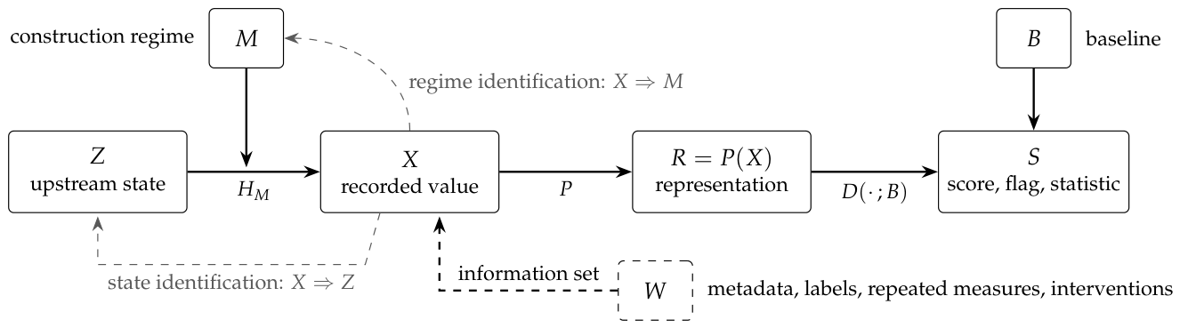
Figure 2.
Attainable sets (filled points) for three rounding regimes: , nearest integer; , nearest even integer; , nearest multiple of five. An observed excludes and ; excludes only; excludes nothing. Because and are subsets of , no observation can exclude by support.
Figure 2.
Attainable sets (filled points) for three rounding regimes: , nearest integer; , nearest even integer; , nearest multiple of five. An observed excludes and ; excludes only; excludes nothing. Because and are subsets of , no observation can exclude by support.
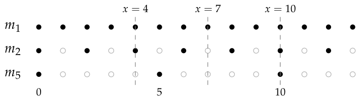

Table 1.
What each literature typically treats as known, what it treats as the target, and where it sits in the chain (2). For numerical diagnostics, the last entry applies when the output is read as evidence about how the observations were produced.
Table 1.
What each literature typically treats as known, what it treats as the target, and where it sits in the chain (2). For numerical diagnostics, the last entry applies when the output is read as evidence about how the observations were produced.
| Literature | Usually treated as known | Primary target | Link in the chain |
|---|---|---|---|
| Coarse data, measurement error | observation model or | Z or | state identification |
| Heaping models | regime family | Z and M jointly | state and regime |
| Mixtures, latent regimes, change points | component family | components, M | regime identification |
| Partial identification | maintained assumptions | identified set | both inverse problems |
| Survey and administrative data | inclusion and collection design | population quantity | sampling vs construction |
| Sufficiency, comparison of experiments | parametric family | information retained | representation P |
| Representation learning | training objective | features | representation P |
| Anomaly detection | representation P, baseline B | unusual geometry | |
| Numerical diagnostics | projection and reference law | conformity of | mechanism–projection–baseline |
Table 2.
The construction classes in real data. Each row locates a trace in U/Q/C/G/A and states the kind of identification output it supports—exact support exclusion, frequency evidence, calibration, separation lost to a representation, information exposed to loss, or nonidentification. The rows are not comparable statistics and are not pooled.
| Layer | Case | Construction | Observable trace | Identification output | Principal limitation |
|---|---|---|---|---|---|
| U | Temperature | whole ∘F converted to tenths ∘C | tenths digit 5 unreachable under whole ∘F | any digit 5 support-excludes whole ∘F; its absence favors whole ∘F by frequency | native ∘C has broader support; absence of 5 is frequency evidence |
| Q | NHANES | mercury protocol records to even mmHg | every reading even | consistent with the even rule; nearest-integer alternative disfavored by frequency | nested supports; instrument comparability assumed |
| C | Genome | codon triplets | CDS length | known biological constraint recovered; a calibration | answer fixed in advance |
| C | Check digits | mod-11 checksum | transpositions fail the check | fault regimes separated exactly in X; inseparable after histogram P | specification-grounded |
| C | Marathon | published qualifying times | notch below the standard | frequency evidence for a threshold response | estimated counterfactual; selected field; 2012 null |
| G | Seawater | sound speed computed by formula | archive reproduced from | near-exact reproduction: strong evidence the column is composed; anomaly comparison cited | external anomaly cited, not recomputed |
| A | Tide gauges | ordered water-level record | M2 amplitude at a fixed period | ordered-record signal that no marginal P preserves; not an observed A regime | upstream physical structure, not a recording regime |
| — | Federal obligations | mixed, unlabeled | cents spikes; zero-cent mass | descriptive form in X; no substantive regime identified | amount choice and recording mechanism confounded |
Disclaimer/Publisher’s Note: The statements, opinions and data contained in all publications are solely those of the individual author(s) and contributor(s) and not of MDPI and/or the editor(s). MDPI and/or the editor(s) disclaim responsibility for any injury to people or property resulting from any ideas, methods, instructions or products referred to in the content. |
© 2026 by the authors. Licensee MDPI, Basel, Switzerland. This article is an open access article distributed under the terms and conditions of the Creative Commons Attribution (CC BY) license (http://creativecommons.org/licenses/by/4.0/).
Copyright: This open access article is published under a Creative Commons CC BY 4.0 license, which permit the free download, distribution, and reuse, provided that the author and preprint are cited in any reuse.