

Submitted:
03 October 2026
Posted:
07 October 2026
You are already at the latest version
Abstract
Generalizing a distribution can be achieved by inserting one or more new parameters to the baseline distribution. The author deliberates this methodology to build, Weibull Median Based Unit Rayleigh {Y} family of distributions. The author applies the approach of the T-X{Y} family to add more than one parameter to the baseline distribution Median Based Unit Rayleigh (MBUR) defined on the unit interval with one parameter b > 0. The generator distribution is the Weibull distribution with the two parameters, c & ξ > 0, the shape and scale parameters respectively as will be explained in the paper. The author consumed different link distributions or Y distributions in the form of the quantile function of this link distribution to link the baseline distribution, the MBUR, to the generator distribution, the Weibull distribution. The link distributions deployed are the Lomax, Dagum, exponential, exponentiated exponential and the Log Logistic distributions. This technique results in new different distributions with different number of parameters, as will be discussed in the paper. For each new distribution, the author derived the PDF, CDF, quantile and hazard functions as well as the raw moments. The author expands some of the PDFs in a linear series expansion that is simple and does not require special function. This makes the computational statistics for the raw moments easier and simpler. The supplementary material associated with the paper contains figures for the PDF, CDF and the Hazard functions. Real data analysis reveals correlation between the parameters of the new distributions. The author clarified this by comparing the fitness of the new distributions to the same dataset, rate of recovery from COVID 19 in Spain, to wonder whether this correlation is data dependent or distribution dependent or mix and interaction between both the data and the distribution.
Keywords:
generalized Weibull-MBUR-{Lomax}
; Weibull-MBUR-{Dagum}
; Weibull-MBUR-{exponential}
; Weibull-MBUR-{exponentiated-exponential}
; Weibull-MBUR-{log-logistic}
Introduction
Generalization of a distribution can be deployed on a continuous distribution whether defined on a bounded interval like the unit interval or on an unbounded interval spanning or the spanning the interval using different approaches. In the literatures, numerous authors created generalization by launching families like the beta generated family of distribution BG-distributions which is manifested as a generalization of the distribution of the order statistics like Beta-normal (Eugene et al., 2002), Beta-cauchy (Alshawarbeh et al., 2013), Beta Frechet (Barreto-Souza et al., 2008), Beta-Pareto (Akinsete et al., 2008), Beta-generalized exponential (Barreto-Souza et al., 2010), Beta-Exponential (Nadarajah & Kotz, 2006), Beta-Weibull (Lee et al., 2007), Beta-modified Weibull (Silva et al., 2010), and Beta-Gumbel (Nadarajah & Kotz, 2004). Also the Kumaraswamy generated distributions, (Kw-G) distributions, are distributions that make use of the Kumaraswamy distribution to create new distributions. A few number of them to be referenced are Kumaraswamy-normal (Cordeiro & De Castro, 2011), Kumaraswamy-Gumbel (Cordeiro et al., 2012), Kukaraswamy-Pareto (Bourguignon et al., 2013), and Kumaraswamy-gamma (Cordeiro & De Castro, 2011). Although, the BG-distributions and KwG-distributions use the Beta and Kumaraswamy distributions as the generator and both are defined on the unit interval, (Alzaatreh et al., 2013) introduced a broad-spectrum method allowing to use any continuous PDF as a generator. Let be a PDF of a random variable defined on the interval which is . Let be a function of of any random variable so that it fulfils the conditions and is differential and monotonically non decreasing and as and as so the CDF of a new family of distribution can be defines as , and the corresponding PDF is . This family was named as transformed-transformer, where the is the transformer that transformed the into a new CDF, . This was suggested to be standard quantile function for some well-known standard distributions like the standard exponential, standard Weibull, standard log-logistic, and the standard Dagum. Also (Lee et al., 2013) used exponentiated CDF of x, , in these quantiles. (Aljarrah et al., 2014) extended this approach by applying , where Q is a quantile of the Y variable that act like a link between the X baseline distribution and the T generator distribution. Here the addition of the new parameters come from considering the Y distribution as any continuous distribution with specific parameters and not a standard distribution. This approach yields the following CDF and PDF
, the new PDF can also be written as
The derivative of the quantile function is the reciprocal of the PDF at specified value say (x), and the following formulas show why. For a specified distribution of Y variable with CDF and quantile evaluated at (x) , ,differentiating both sides, , yields, , and consequently The generalization of the distributions defined on the unit interval can be accomplished by different techniques like the power transformation to output the power Johnson B (Cancho et al., 2020), power Generalized Johanson SB (Gallardo et al., 2022), and power unit inverse Lindley distribution (Gemeay et al., 2024). Another famous technique is the T-X family of distributions which can create generalization of the unit distribution. Some of the distributions in this category are the transmuted power unit inverse Lindley distribution (Eldessouky et al., 2025), Kumaraswamy generalized family of distribution (Tahir et al., 2020), and the generalized unit half logistic geometric distribution (Nasiru et al., 2023). Deploying the T-X {Y} approach which is an extension of the T-X method, (Osatohanmwen et al., 2021) explained the generalized family of T-Kumaraswamy family of distributions with the following distributions: Weibull-Kumaraswamy {exponential}, log-logistic-Kumaraswamy {exponential}, exponential-kumaraswamy{log-logistic}, normal-kumaraswamy {logistic}, and logistic-Kumaraswamy {extreme-value}. Also, (Sudsila et al., 2022) elucidated the generalized family of distribution based on T-Topp Leone {Y} family of distributions and the examined distributions were: Weibull-TL-{exponential}, log-logistic-TL{exponential}, Logistic-TL{extreme-value}, exponential-TL{log-logistic}, and normal-TL{logistic}. The author developed the generalized odd median based unit Rayleigh using the general formula of the order statistics (Attia, 2025)
Various authors elucidated the generalization of distributions on unit interval like:(McDonald, 2008) demonstrated the generalized beta distribution of the first kind, (Carrasco et al., 2010) clarified generalized Kumaraswamy distribution, (El-Sherpieny & Ahmed, 2014) illuminated Kumaraswamy-Kumaraswamy distribution, (Elgarhy et al., 2018) exemplified exponentiated generalized Kumaraswamy distribution. Some of the major importance of the unit distributions are making benefit of these distributions as conjugate prior to a certain well recognized discrete distributions in Bayesian statistics and inference, besides accommodating different shapes and models of the percentages, proportions, fractions and ratios with random conduct.
To the best of the author knowledge the Weibull-MBUR{Lomax}, Weibull-MBUR {Dagum}, Weibull-MBUR {exponential}, Weibull-MBUR {exponentiated-exponential}, Weibull-MBUR {Log Logistic}, were not discussed before in the literature. The author chosen the Weibull as a generator because it has a well closed form of the CDF that makes the derivation of the quantile function of the new distribution easy to obtain. Also the raw moments of the Weibull distribution are easy to obtain even if requiring the gamma special function. The chosen link distributions result in a Y variable, , that is within the support of the Weibull distribution.
To find the quantile of such new family you follow these steps on the CDF of the new distribution , this approach can be summarized by the following equation, . In other words, the formula , finds the quantile of the generator distribution, , substitutes it into the CDF of the link function , and lastly inserts it into the quantile function of the baseline distribution . That is to say you reverse the processes . This approach can be applied as will be explained in the paper.
This paper discusses five new distributions. For each distribution, the methodology of derivation of the PDF is fully explained, as well as the CDF, quantile, and hazard functions. The raw moments are expounded using two different approaches. One approach depends on series linear expansion of the new PDF and this is illustrated for the Weibull-MBUR{Lomax} and the Weibull-MBUR {Dagum}. The other approach relies on isolating the x variable and taking the expectation of the rth raw moment which depends on the raw moments of the generator, the Weibull distribution, as will be demonstrated in the paper. Moreover, real data analysis is used to fit the different distributions and to compare the existence of correlation between the parameters for each distribution.
Methodology (Methods and Materials)
Derivation of Weibull-MBUR {Y} Family of Distributions
The generator distribution is the Weibull (the distribution of the T variable), the baseline distribution is the MBUR (the distribution of the X variable) and the distribution which can be considered as a link between the T and X distributions is the distribution of the Y variable (the distribution of the quantile function).
The Weibull Distribution has the following PDF, CDF and quantile functions , , , respectively, where; , , the shape and scale parameters are respectively.
The MBUR Distribution has the following PDF, CDF, and quantile functions respectively: , ,
, respectively, where , , and the shape parameter is
1. Weibull-MBUR {Lomax} Distribution
1.1. Lomax Link Distribution
The Lomax Distribution has the following PDF, CDF, and quantile functions , , , respectively, where; , , the shape and scale parameters are respectively
Use the approach discussed by Aljarrah 2014 as shown in the following steps to derive the PDF.
Step 1: substitute the CDF of MBUR into the quantile function of the link distribution (quantile function of Y), to obtain the t variable.
Step 2: substitute this T variable into the PDF of the Weibull distribution
Step 3: get the derivative of the quantile function which is the reciprocal of the PDF of the quantile distribution:
Step 4: substitute into the equation of :
, where is bigger than one and so can be written as .
And when is multiplied by the denominator it can be written as
After rearrangement and for convenient the in the following PDF and CDF where x is defined on the unit interval:
To derive the substitute the t variable into the CDF of the generator Weibull distribution
Quantile function: to derive the quantile function follow the steps
Step 1: Take the quantile of the generator, or
Step 2: Substitute this quantile in the CDF of the link distribution, ,
Step 3: Substitute the result and call it, Z; into the quantile function of the baseline distribution MBUR distribution. This will give the same result as taking the inverse of the
Another approach that can be deployed to obtain the quantile function ofis by taking the inverse of the:
, solve for x yields the following equation , the left hand side is the CDF of the baseline distribution MBUR and the right hand side is a constant, which is the z, and z is . Solving the third degree polynomial for its root yields the variable or the quantile function for the new distribution is
The hazard function is defined as
Theorem 1: The rth moment for the new distribution can be expressed in the formulas according to the scale parameter of the link function or the Lomax distribution as will be shown in the proof
Proof: start with the t variable and isolate the x at one side
so this gives use the generalized binomial theory on the left hand side
this gives
Take the rth power of both sides
, 0 <
Use the generalized binomial theory to expand the
Use the generalized binomial theory to expand the , here there are two cases
First case:
Take expectation of both sides
is the uth raw moment of the Weibull variable (the t variable)
The proof of the :
, use change of variable, so and
is the raw moment of the Weibull variable (the t variable).
Second case: ,
factor out the so , then expand the using the generalized binomial theorem then take the expectation.
where the
Theorem 2: linear series expansion of this new pdf , is applied to the exponent term and each of the power terms, using the generalized binomial expansion and Pochhammer falling factorial
Proof:
, is the CDF for MBUR and it is monotonically increasing function and it is , so can be expanded using the generalized binomial theory. Also to be noticed that so
and is less than 1 so using the generalized binomial theory
For the power term , is less than 1 so generalized binomial theory can be applied on
another generalized binomial expansion be applied on the
For the term applying binomial expansion gives
Assembling both power terms together
The exponent term can be expanded as
Now put the all the parts together
Where
Integrate this series expansion by integrating the x from 0 to 1 because the support of the distribution is the support of the MBUR so the integral will pass to the x
This gives
Theorem 3: the hth non-central moments are given by the following formula:
Proof:
In the supplementary material, the author depicts different figures illustrating the behavior of the distribution as regards the PDF, CDF and hazard functions. The PDF can exhibit bathtub, increasing and decreasing, right skewed and left skewed shapes and other different shapes. The hazard rate is mainly increasing and J shaped.
2. Weibull-MBUR {Dagum} Distribution
2.1. Dagum Link Distribution
The Dagum Distribution has the following PDF, CDF, and quantile functions , , , respectively, where; , , the two shape and scale parameters are respectively.
Use the approach discussed by Aljarrah 2014 as shown in the following steps to derive the PDF.
Step 1: substitute the CDF of MBUR into the quantile function of the link distribution (quantile function of Y), to obtain the t variable.
Step 2: substitute this T variable into the PDF of the Weibull distribution
Step 3: get the derivative of the quantile function which is the reciprocal of the PDF of the quantile distribution:
Step 4: substitute into the equation of :
, where
As long as for the following term can be written as
After rearrangement and for convenient the in the following PDF and CDF where x is defined on the unit interval:
To derive the , substitute the t variable into the CDF of the Weibull distribution
To find the quantile function apply the following steps.
Step 1: Take the quantile of the generator,
Step 2: Substitute this quantile in the CDF of the link distribution. ,
Step 3: Substitute the result and call it, Z; into the quantile function of the baseline distribution MBUR distribution. This will give the same result as taking the inverse of the .
Another approach that can be deployed to obtain the quantile function of is by taking the inverse of the : , solve for x yields the following equation , the left hand side is the CDF of the baseline distribution MBUR and the right hand side is a constant, which is the z, and z is . Solving the third degree polynomial for its root yields the variable or the quantile function for the new distribution is
The hazard function is defined as
Theorem 4: the rth moment for the new distribution is presented in the formulas according to the shape and scale parameters of the link function or the Dagum random variable, this will be illustrated in the proof.
Proof: start with the t variable and isolate the x on one side
this gives
this gives
use generalized binomial expansion
the following step is
so
Take the rth power of both sides
there are two cases:
First case: if
Use the generalized binomial theory to expand the
Take the expectation of both sides
is the sth raw moment of the Weibull variable (the t variable), where in other words , . That is to say sth moment index whether 1 ,2 3, or 4 should lie between the 0 and the ratio between the shape parameter of the Weibull random variable and shape parameter of the Dagum random variable
second case: if , factor out the then distribute the power then apply the generalized binomial theorem
then expand by applying the generalized binomial theorem and then taking the expectation
Theorem 5: linear series expansion of this new pdf , is applied to the exponent term and each of the power terms, using the generalized binomial expansion and Pochhammer falling factorial
Proof: using the series expansion for the power terms; the first power term
, is the CDF for MBUR and it is monotonically increasing function can be expanded using the generalized binomial theory. Also to be noticed that so the first power term can be expanded using generalized binomial theorem as
The second power term where is <1 for
The exponent term can be expanded as
Now put the three parts together
Integrate this series expansion by integrating the x from 0 to 1 because the support of the distribution is the support of the MBUR so the integral will pass to the x
This gives
Theorem 6: the rth non-central moments are given by the following formula:
Proof:
In the supplementary material, the author depicts different figures illustrating the behavior of the distribution as regards the PDF, CDF and hazard functions. The PDF can exhibit reversed J shaped, increasing and decreasing, N shape, left skewed and right skewed and other different shapes. The hazard rate is mainly increasing and J shaped.
3. Weibull-MBUR {Exponential} Distribution
3.1. Exponential Link Distribution
The exponential Distribution has the following PDF, CDF, and quantile functions , , , respectively, where; , , the scale parameter is respectively.
Use the approach discussed by Aljarrah 2014 as shown in the following steps to derive the PDF.
Step 1: substitute the CDF of MBUR into the quantile function of the link distribution (quantile function of Y), to obtain the t variable.
Step 2: substitute this T variable into the PDF of the Weibull distribution
Step 3: get the derivative of the quantile function which is the reciprocal of the PDF of the quantile distribution:
Step 4: substitute into the equation of :
, where
The PDF is
The CDF is
To find the quantile follow the steps.
Step 1: take the quantile of the generator, or
Step 2: Substitute this quantile in the CDF of the link distribution. ,
Step 3: Substitute the result and call it, Z; into the quantile function of the baseline distribution MBUR distribution. This will give the same result as taking the inverse of the .
Another approach that can be deployed to obtain the quantile function of is by taking the inverse of the , solving for x yields the following equation, , the left hand side is the CDF of the baseline distribution MBUR and the right hand side is a constant, which is the z, and z is . Solving the third degree polynomial for its root yields the variable or the quantile function for the new distribution which is
The hazard function is defined as
Theorem 7: the rth non-central moments are given by the following formula
Proof: Starting with the t variable
then isolating the x as shown in the following steps
this gives
this gives
this gives
using the binomial expansion
this gives
Take the rth power of both sides
Use the generalized binomial theory to expand the
Then expand the exponent
Take expectation of both sides
is the uth raw moment of the Weibull variable (the t variable)
In the supplementary material, the author depicts different figures illustrating the behavior of the distribution as regards the PDF, CDF and hazard functions. The PDF can exhibit reversed J shaped, increasing and decreasing, N shape, left skewed and right skewed shapes and other different shapes. The hazard function is mainly increasing, bathtub or J shape.
4. Weibull-MBUR {Exponentiated-Exponential} Distribution
4.1. Exponentiated-Exponential Link Distribution
The exponentiated exponential Distribution has the following PDF, CDF, and quantile functions , , , respectively, where; , , the scale and shape parameters are respectively.
Use the approach discussed by Aljarrah 2014 as shown in the following steps to derive the PDF.
Step 1: substitute the CDF of MBUR into the quantile function of the link distribution (quantile function of Y), to obtain the t variable.
Step 2: substitute this T variable into the PDF of the Weibull distribution
Step 3: get the derivative of the quantile function which is the reciprocal of the PDF of the quantile distribution:
Step 4: substitute into the equation of :
, where
The PDF is
The CDF is
To find the quantile follow the steps.
Step 1: take the quantile of the generator, or
Step 2: Substitute this quantile in the CDF of the link distribution.
Step 3: Substitute the result and call it, Z; into the quantile function of the baseline distribution MBUR distribution. This will give the same result as taking the inverse of the .
Another approach that can be deployed to obtain the quantile function of is by taking the inverse of the , solving for x yields the following equation, , the left hand side is the CDF of the baseline distribution MBUR and the right hand side is a constant, which is the z, and z is . Solving the third degree polynomial for its root yields the variable or the quantile function for the new distribution which is
The hazard function is defined as
Theorem 8: the rth non-central moments are given by the following formula
Proof: Starting with the t variable then isolating the x as shown in the following steps
this gives
this gives
this gives
this gives
Expand the using the generalized binomial theory
this gives
Take the rth power of both sides
Use the generalized binomial theory to expand the
Expand the exponent
Take expectation of both sides
In the supplementary material, the author depicts different figures illustrating the behavior of the distribution as regards the PDF, CDF and hazard functions. The PDF can exhibit reversed J shaped, increasing and decreasing, N shape, left skewed and right skewed shapes and other different shapes. The hazard function is mainly increasing and J shaped.
5. Weibull-MBUR {Log Logistic} Distribution
5.1. Log Logistic Link Distribution
The log_logistic Distribution has the following PDF, CDF, and quantile functions , , , respectively, where; , , the scale and shape parameters are respectively.
Use the approach discussed by Aljarrah 2014 as shown in the following steps to derive the PDF.
Step 1: substitute the CDF of MBUR into the quantile function of the link distribution (quantile function of Y), to obtain the t variable.
Step 2: substitute this T variable into the PDF of the Weibull distribution
Step 3: get the derivative of the quantile function which is the reciprocal of the PDF of the quantile distribution:
Step 4: substitute into the equation of :
, where
The PDF is
The CDF is
To find the quantile follow the steps.
Step 1: take the quantile of the generator, or
Step 2: Substitute this quantile in the CDF of the link distribution.
Step 3: Substitute the result and call it, Z; into the quantile function of the baseline distribution MBUR distribution. This will give the same result as taking the inverse of the .
Another approach that can be deployed to obtain the quantile function of is by taking the inverse of the , solving for x yields the following equation, , the left hand side is the CDF of the baseline distribution MBUR and the right hand side is a constant, which is the z, and z is . Solving the third degree polynomial for its root yields the variable or the quantile function for the new distribution which is
The hazard function is defined as
Theorem 9: the rth non-central moments are given by the following formula depending on the scale and shape parameters of the link distribution function as shown in the proof
Proof: Starting with the t variable
then isolating the x as shown in the following steps
this gives
Take the rth power of both sides
Use the generalized binomial theory to expand the there are two cases
First case : if
Take expectation of both sides
is the raw moment of the Weibull variable (the t variable)
Second case : , factor out the so that
then use the generalized binomial theory, then take the expectation
Take expectation of both sides
Theorem 10: linear series expansion of this new pdf , is applied to the exponent term and each of the power terms, using the generalized binomial expansion and Pochhammer falling factorial
Proof:
The PDF is
The power term is expanded as
The power term is expanded as
The exponent term can be expanded as
Assemble all the terms together so the PDF can be represented as
Integrate this series expansion by integrating the x from 0 to 1 because the support of the distribution is the support of the MBUR so the integral will pass to the x
Theorem 11: the rth non-central moments are given by the following formula:
Proof:
In the supplementary material, the author depicts different figures illustrating the behavior of the distribution as regards the PDF, CDF and hazard functions. The PDF can exhibit, J shape and reversed J shaped, increasing and decreasing, M shape, left skewed and right skewed shape and other different shapes. The hazard function shapes show mainly increasing and J shaped appearance.
Results of Real Data Analysis and Discussion
The following is 66 observations of the recovery rate from the COVID 19 patients in Spain: 0.667, 0.5000, 0.5000,0.4286, 0.7500, 0.6531, 0.5161, 0.7895, 0.7689, 0.6873, 0.5200, 0.7251, 0.6375, 0.6078, 0.6289, 0.5712, 0.5923, 0.6061, 0.5924, 0.5921, 0.5592, 0.5954, 0.6164, 0.6455, 0.6725, 0.6838, 0.6850, 0.6947, 0.7210, 0.7315, 0.7412, 0.7508, 0.7519, 0.7547, 0.7645, 0.7715, 0.7759, 0.7807, 0.7838, 0.7847, 0.7871, 0.7902, 0.7934, 0.7913, 0.7962, 0.7971, 0.7977, 0.8007, 0.8038, 0.8289, 0.8322, 0.8354, 0.8371, 0.8387, 0.8456, 0.8490, 0.8535, 0.8547, 0.8564, 0.8580, 0.8604, 0.8628, 0.6586, 0.7070, 0.7963, 0.8516. This dataset was previously discussed by (Ahmed Z. Afify et al., 2022)
These observations have a mean value of 0.7240, a standard deviation value of 0.1086, a skewness value of -0.7214, a kurtosis value of 2.6670, a minimum value at 0.4286, and a maximum value of 0.8628. The 25th quantile is 0.6455, the median is 0.7533, and the 75th quantile is 0.7977. The author used fmincon function in MATLAB to estimate the parameters.
The five new distribution was compared with the Beta, Kumaraswamy, Topp –Loene distribution, Unit Lindley and Generalized Odd Median Based Unit Rayleigh type I (GOMBUR-I) and GOMBUR type 2 (BOMBUR-II) as regards fitting the data. The results are shown in Table 1. The Log Likelihood (LL) are nearly equal between the Beta, Kumaraswamy and GOMBUR type 1 and 2. Also the AIC, CAIC, BIC, and HQIC are nearly equal. Moreover, the KS statistics are nearly equal. The Kumaraswamy is the best distribution to fit the data followed by GOMBUR-I and GOMBUR-II and lastly the Beta distribution. If considering the variance-covariance matrix and its determinant, the GOMBUR-I followed by GOMBUR-II are better than Kumaraswamy because they have less values. The baseline distribution MBUR did not fit the data as shown from LL and other statistical indices. Topp-Loene distribution and Unit Lindley distribution did not fit the data as shown in Table 2.
Table 3 shows the statistical indices for the five distributions. For each distribution, the estimated parameters are recorded with the corresponding standard error for each estimated parameter. The AIC, CAIC, BIC and the HQIC are recorded for each distribution. The Log Likelihood is also recorded. The KS statistics and the associated p-value are also mentioned. The determinant (Determ.) of the matrix is lastly recorded. Table 4 shows the 95% confidence interval for the estimated parameters for each of the five distributions. The new distributions have LL higher than that of the previous distributions in Table 1, the best is recorded from Weibull-MBUR{Lomax} distribution. The AIC, CAIC, BIC and HQIC are also better for the Weibull-MBUR{Lomax} than the indices of the other new distributions and the indices of the previous distributions shown in Table 1. Although the statistical indices reflect better fitting of the distribution to the data, the correlation between the estimated parameters of the Weibull-BMUR{Lomax} is very high. It is obvious that the addition of new parameters to the baseline distribution MBUR enables the baseline distribution to fit the data and accommodate the skewness and the shape of the data. The baseline distribution could not accommodate this skewness and did not fit the data well. Generalization, by using different derivation method like GOMBUR-I and GOMBUR-II and by using the T-X{Y} technique with the application of Weibull distribution as the generator distribution and with the utilization of different link {Y} distributions, enhances the performance of the new generalized distributions to accommodate the shape of the data. The 95% confidence interval is wide because the variance and hence the standard errors for the estimated parameters are high, which is depicted from Table 3. Figure 1, Figure 2, Figure 3, Figure 4 and Figure 5 shows the fitted PDFs and CDFs for the new distributions.
For the Weibull-MBUR{Lomax} distribution, the followings are the matrix and correlation matrix. The columns of each matrix are the parameters in the following sequence: , , , , , and consequently the rows are the transpose of this sequence.
For the Weibull-MBUR{Dagum} distribution, the followings are the matrix and correlation matrix. The columns of each matrix are the parameters in the following sequence: , , , , , , and consequently the rows are the transpose of this sequence.
For the Weibull-MBUR {exponential} distribution, the followings are the matrix and correlation matrix. The columns of each matrix are the parameters in the following sequence: , , , , and consequently the rows are the transpose of this sequence.
For the Weibull-MBUR {exponentiated exponential} distribution, the followings are the matrix and correlation matrix. The columns of each matrix are the parameters in the following sequence: , , , , and consequently the rows are the transpose of this sequence.
For the Weibull-MBUR {Log Logistic} distribution, the followings are the matrix and correlation matrix. The columns of each matrix are the parameters in the following sequence: , , , , and consequently the rows are the transpose of this sequence.
The correlations between the parameters of the Weibull-MBUR {Lomax} distribution are very high and positively correlated. It has a nearly zero determinant of the estimated variance-covariance matrix of its estimated parameter (5.6073e-13).
Although the determinant of the estimated variance-covariance matrix of the estimated parameters of the Weibull-MBUR {Dagum} distribution is 0.1637, some of the parameters depict high positive correlation (the parameter shows perfect correlation with the , and ; what’s more to say is that demonstrates perfect correlation with and ; likewise expresses perfect correlation with ), while the shows high negative correlation with .
The Weibull-MBUR {exponential} distribution has a variance-covariance matrix whose determinant is 1.4252e-8 and the parameters of the distribution display high correlation. The parameter is positively moderately correlated with and is positively highly correlated with whilst negatively highly correlated with . The parameter is positively moderately correlated with but negatively moderately correlated with . The is negatively highly correlated with .
The determinant of the estimated variance-covariance matrix of the estimated parameters of the Weibull-MBUR {exponentiated-exponential} is 8.019e-18. The parameter is negatively highly correlated with . Similarly, c is negatively highly correlated with .
The estimated variance-covariance matrix of the estimated parameters of the Weibull-MBUR {Log Logistic} distribution has a determinant equal 58863. The parameter is negatively moderately correlated with and . The parameter is positively moderately correlated with . Likewise, the is positively highly correlated with .
The correlations between parameters may be inherited from the distributions components of the T-X {Y} system constructing the new distributions. Though the imposed effect of the data cannot be ruled out and this allegation need to be evaluated by further simulation studies.
Conclusion
The new generalized distributions have their parameters from the sequential insertion of the parameters of the component distributions, one shape parameter from the baseline distribution the (MBUR), the different scale and shape parameters from the different link{Y] distributions, the distributions of the quantile function, and the scale and shape parameters of the generator distribution, the Weibull distribution. These permit the curve of the PDF to fit and twist with the skewed shape of the data and hence fit the data well as was shown from the Figure 1, Figure 2, Figure 3, Figure 4 and Figure 5 of the shape of the fitted PDFs and fitted CDFs. The add-on of these new parameters decreases the covariance between some of the parameters although some parameters may exhibit high correlation. Moreover, the addition of the parameters improves the indices of validation like the AIC, corrected-AIC, BIC and HQIC over the indices obtained from fitting the baseline distribution. It also augments the Log-Likelihood. In some cases, the baseline distribution may not fit the data but after the generalization and the addition of the new parameters the new generalized distribution fit the data well. In this case study and real data analysis, the baseline distribution did not fit the data but the new different generalized distributions fit the data well. As illustrated from the discussion about the correlations between the estimated parameters extra simulation studies are needed to reveal the claim whether these correlations are distributions or data driven and whether the correlations are inherited from the components distributions of the T-X {Y} system assembling the new distributions.
Future Work
Utilizing other link functions or quantile distributions like the logistic and generalized logistic distributions that output quantiles spanning the entire line with the use of different generators other than the Weibull distributions whose support spans like the normal distribution and Cauchy distribution with the same baseline distribution the BMUR, to compare these newly built distributions and to see if the addition of new parameters imposes correlations and to what extent the correlations exist and to evaluate the accusation of passing correlations from the components of the T-X {Y} system family of distributions to the newly created distributions. The normal distribution has two parameters the mean and the sigma square, they are well-known to be independent. The Cauchy distribution also has a location and scale parameters. Besides, these simulation studies will reveal how the correlations affect the 95% confidence interval. So extra simulation studies are required to evaluate these issues and remedies for them.
Supplementary Materials
The following supporting information can be downloaded at the website of this paper posted on Preprints.org.
Funding
No funding resource. No funding roles in the design of the study and collection, analysis, and interpretation of data and in writing the manuscript are declared.
Ethics approval and consent to participate
Not applicable.
Consent for publication
Not applicable.
Availability of data and material
Not applicable. Data sharing not applicable to this article as no datasets were generated or analyzed during the current study.
Competing interests
The author declares no competing interests of any type.
Authors’ contribution
AI carried the conceptualization by formulating the goals, aims of the research article, formal analysis by applying the statistical, mathematical and computational techniques to synthesize and analyze the hypothetical data, carried the methodology by creating the model, software programming and implementation, supervision, writing, drafting, editing, preparation, and creation of the presenting work.
Acknowledgments
Not applicable.
References
- Afify, A.Z.; Nassa, Mazen; Kumard, Devendra; Cordeiro, Gauss M. A new unit distribution: Properties, inference, and applications. Electron. J. Appl. Stat. Anal. 2022, Vol. 15(Issue 02), 460–484. [Google Scholar]
- Akinsete, A.; Famoye, F.; Lee, C. The beta-Pareto distribution. Statistics 2008, 42(6), 547–563. [Google Scholar] [CrossRef]
- Aljarrah, M. A.; Lee, C.; Famoye, F. On generating T-X family of distributions using quantile functions. J. Stat. Distrib. Appl. 2014, 1(1), 24. [Google Scholar] [CrossRef]
- Alshawarbeh, E.; Famoye, F.; Lee, C. Beta-Cauchy Distribution: Some Properties and Applications. J. Stat. Theory Appl. 2013, 12(4), 378. [Google Scholar] [CrossRef]
- Alzaatreh, A.; Lee, C.; Famoye, F. A new method for generating families of continuous distributions. METRON 2013, 71(1), 63–79. [Google Scholar] [CrossRef]
- Attia, I. M. The new generalized odd Median Based Unit Rayleigh. Front. Appl. Math. Stat. 2025, 11, 1648127. [Google Scholar] [CrossRef]
- Barreto-Souza, W.; Cordeiro, G. M.; Simas, A. B. Some results for beta Fréchet distribution. arXiv 2008, arXiv:0809.1873. [Google Scholar] [CrossRef]
- Barreto-Souza, W.; Santos, A. H. S.; Cordeiro, G. M. The beta generalized exponential distribution. J. Stat. Comput. Simul. 2010, 80(2), 159–172. [Google Scholar] [CrossRef]
- Bourguignon, M.; Silva, R. B.; Zea, L. M.; Cordeiro, G. M. The Kumaraswamy Pareto distribution. J. Stat. Theory Appl. 2013, 12(2), 129. [Google Scholar] [CrossRef]
- Cancho, V. G.; Bazán, J. L.; Dey, D. K. A new class of regression model for a bounded response with application in the study of the incidence rate of colorectal cancer. Stat. Methods Med. Res. 2020, 29(7), 2015–2033. [Google Scholar] [CrossRef] [PubMed]
- Carrasco, J. M. F.; Ferrari, S. L. P.; Cordeiro, G. M. A New Generalized Kumaraswamy Distribution; arXiv, 2010. [Google Scholar] [CrossRef]
- Cordeiro, G. M.; De Castro, M. A new family of generalized distributions. J. Stat. Comput. Simul. 2011, 81(7), 883–898. [Google Scholar] [CrossRef]
- Cordeiro, G. M.; Nadarajah, S.; Ortega, E. M. M. The Kumaraswamy Gumbel distribution. Stat. Methods Appl. 2012, 21(2), 139–168. [Google Scholar] [CrossRef]
- Eldessouky, E. A.; Hassan, O. H. M.; Aloraini, B.; Elbatal, I. Modeling to medical and economic data using: The transmuted power unit inverse Lindley distribution. Alex. Eng. J. 2025, 113, 633–647. [Google Scholar] [CrossRef]
- Elgarhy, M.; Haq, M. A. U.; Ul Ain, Q. Exponentiated Generalized Kumaraswamy Distribution with Applications. Ann. Data Sci. 2018, 5(2), 273–292. [Google Scholar] [CrossRef]
- El-Sherpieny, E.-S.; Ahmed, M. On the Kumaraswamy Kumaraswamy distribution. Int. J. Basic Appl. Sci. 2014, 3(4), 372–381. [Google Scholar] [CrossRef]
- Eugene, N.; Lee, C.; Famoye, F. BETA-NORMAL DISTRIBUTION AND ITS APPLICATIONS. Commun. Stat.-Theory Methods 2002, 31(4), 497–512. [Google Scholar] [CrossRef]
- Gallardo, D. I.; Bourguignon, M.; Gómez, Y. M.; Caamaño-Carrillo, C.; Venegas, O. Parametric Quantile Regression Models for Fitting Double Bounded Response with Application to COVID-19 Mortality Rate Data. Mathematics 2022, 10(13), 2249. [Google Scholar] [CrossRef]
- Gemeay, A. M.; Alsadat, N.; Chesneau, C.; Elgarhy, M. Power unit inverse Lindley distribution with different measures of uncertainty, estimation and applications. AIMS Math. 2024, 9(8), 20976–21024. [Google Scholar] [CrossRef]
- Lee, C.; Famoye, F.; Alzaatreh, A. Y. Methods for generating families of univariate continuous distributions in the recent decades. WIREs Comput. Stat. 2013, 5(3), 219–238. [Google Scholar] [CrossRef]
- Lee, C.; Famoye, F.; Olumolade, O. Beta-Weibull Distribution: Some Properties and Applications to Censored Data. J. Mod. Appl. Stat. Methods 2007, 6(1), 173–186. [Google Scholar] [CrossRef]
- McDonald, J. B. Some Generalized Functions for the Size Distribution of Income. In Modeling Income Distributions and Lorenz Curves; Chotikapanich, D., Ed.; Springer New York, 2008; pp. 37–55. [Google Scholar] [CrossRef]
- Nadarajah, S.; Kotz, S. The beta Gumbel distribution. Math. Probl. Eng. 2004, 2004(4), 323–332. [Google Scholar] [CrossRef]
- Nadarajah, S.; Kotz, S. The beta exponential distribution. Reliab. Eng. Syst. Saf. 2006, 91(6), 689–697. [Google Scholar] [CrossRef]
- Nasiru, S.; Chesneau, C.; Abubakari, A. G.; Angbing, I. D. Generalized Unit Half-Logistic Geometric Distribution: Properties and Regression with Applications to Insurance. Analytics 2023, 2(2), 438–462. [Google Scholar] [CrossRef]
- Osatohanmwen, P.; Oyegue, F. O.; F., E.; B., A. A New Family of Generalized Distributions on the Unit Interval: The T− kumasatwamy Family of Distributions. J. Data Sci. 2021, 219–237. [Google Scholar] [CrossRef]
- Silva, G. O.; Ortega, E. M. M.; Cordeiro, G. M. The beta modified Weibull distribution. Lifetime Data Anal. 2010, 16(3), 409–430. [Google Scholar] [CrossRef] [PubMed]
- Sudsila, P.; Thongteeraparp, A.; Aryuyuen, S.; Bodhisuwan, W. The Generalized Distributions on the Unit Interval based on the T-Topp-Leone Family of Distributions. Trends Sci. 2022, 19(19), 6186. [Google Scholar] [CrossRef]
- Tahir, M. H.; Hussain, M. A.; Cordeiro, G. M.; El-Morshedy, M.; Eliwa, M. S. A New Kumaraswamy Generalized Family of Distributions with Properties, Applications, and Bivariate Extension. Mathematics 2020, 8(11), 1989. [Google Scholar] [CrossRef]
Figure 1.
shows that the data exhibit slight negative skewness. The Weibull MBUR {Lomax} PDF and CDF fit the data well.
Figure 1.
shows that the data exhibit slight negative skewness. The Weibull MBUR {Lomax} PDF and CDF fit the data well.
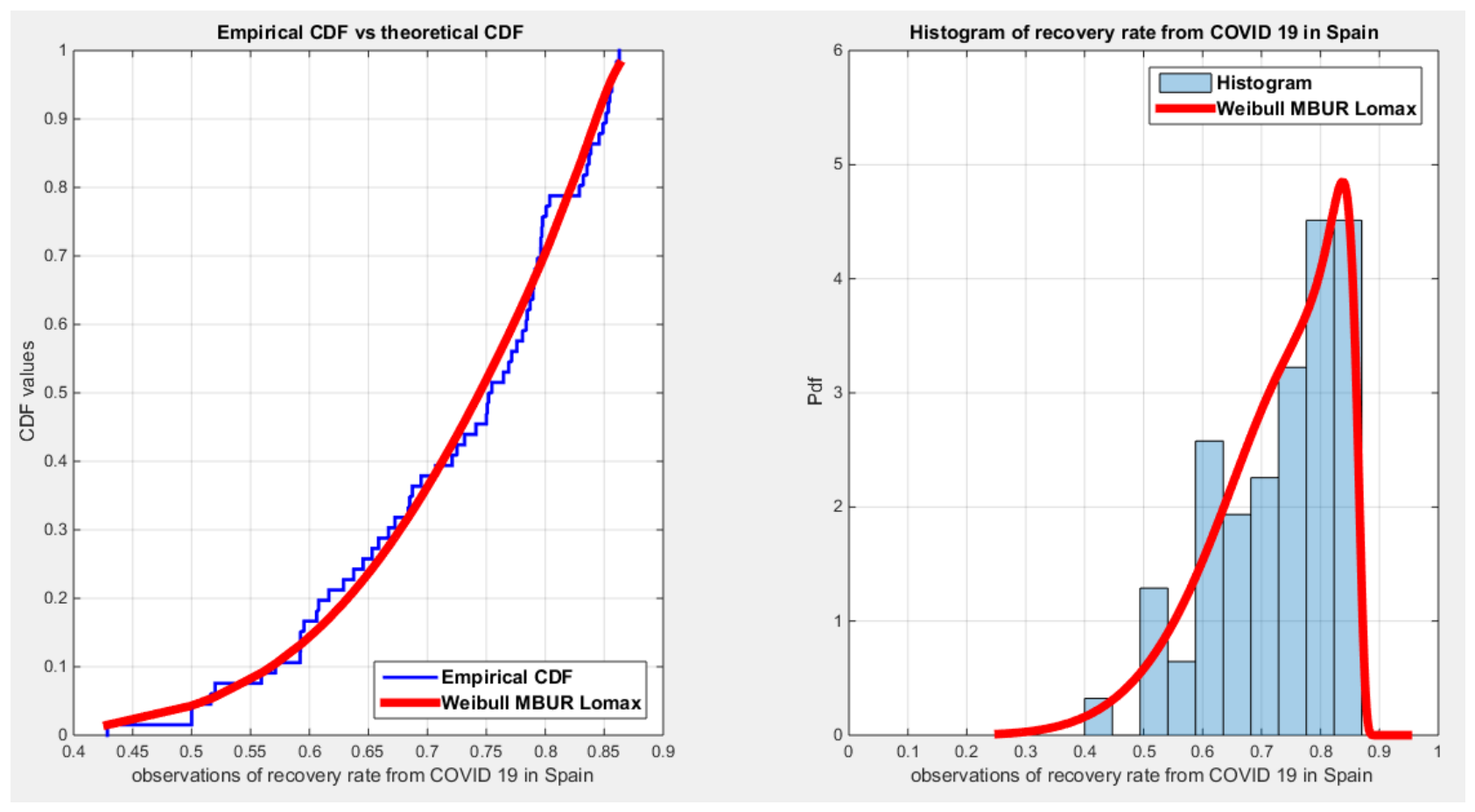
Figure 2.
shows that the Weibull MBUR {Dagum} PDF and CDF fit the data well.
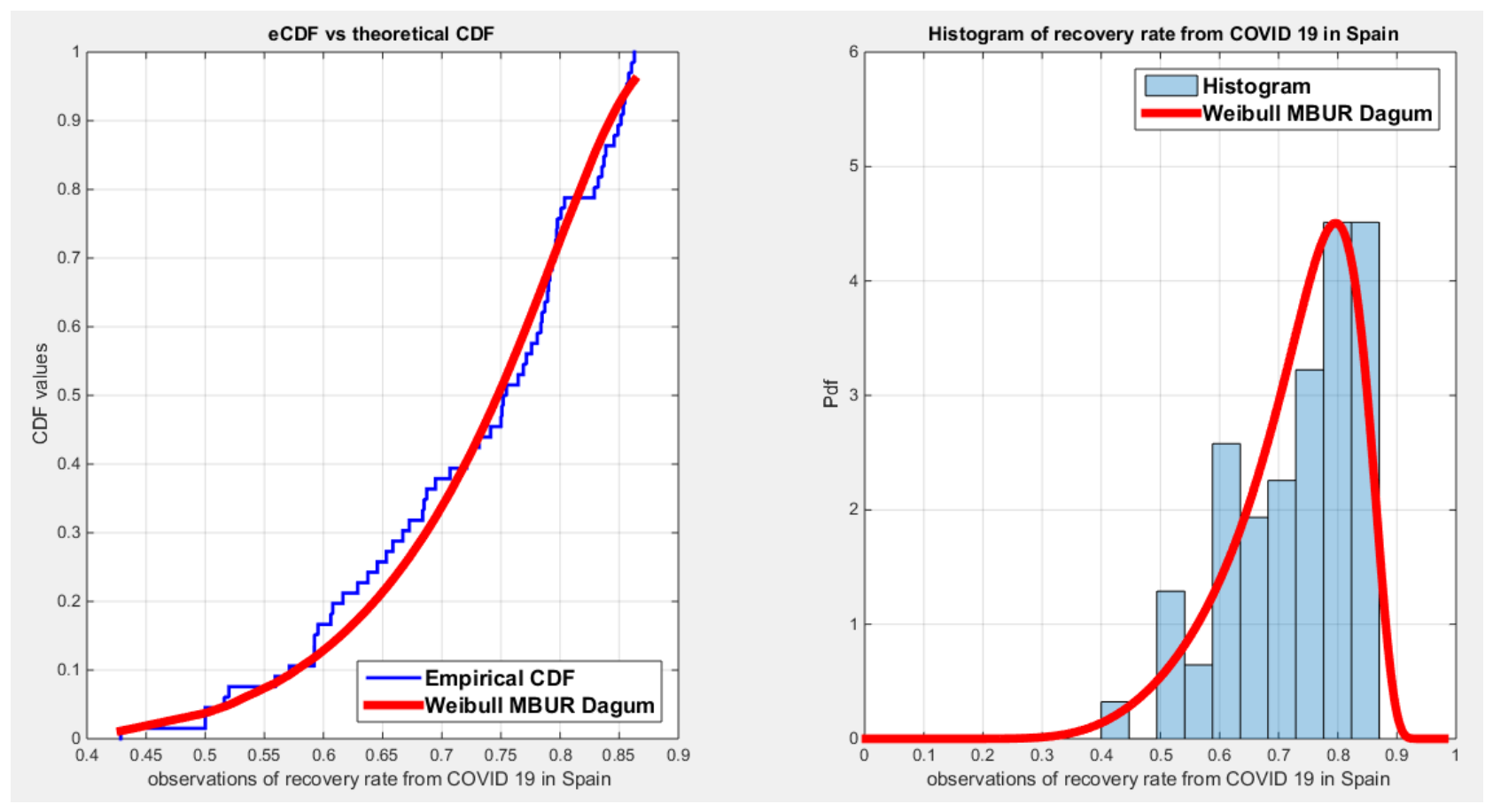
Figure 3.
shows that the Weibull MBUR {exponential} PDF and CDF fit the data well.
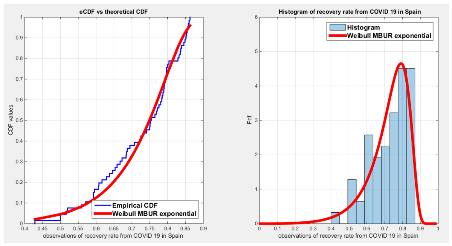
Figure 4.
shows that the Weibull MBUR {exponentiated-exponential} PDF and CDF fit the data well.
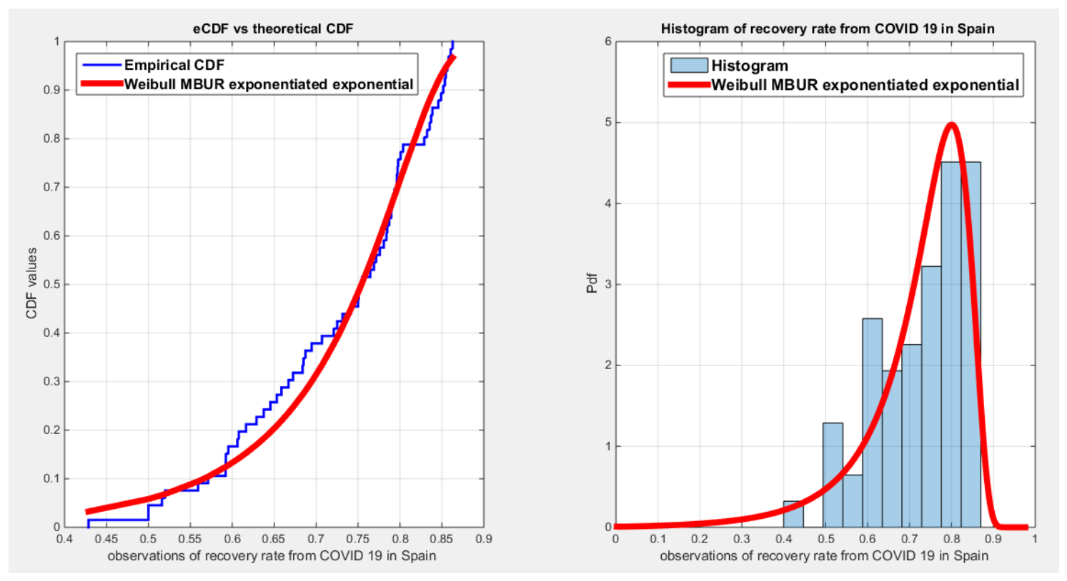
Figure 5.
shows that the Weibull MBUR {Log Logistic} PDF and CDF fit the data well.
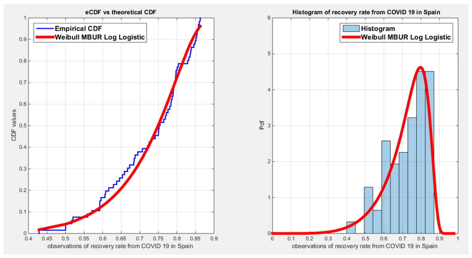

Table 1.
statistical indices for the Beta, Kumaraswamy, MBUR, GOMBUR-I and GOMBUR-II.
| Beta | Kumaraswamy | MBUR | GOMBUR-I | GOMBUR-II | |
| parameter | |||||
| Standard error |
2.8439 for | 0.9469for | 0.0281for | 0.8554 for | 1.7108 for |
| 1.1949 for | 2.0186 for | 0.0191 for | 0.0191 for | ||
| LL | 57.5743 | 58.8343 | 46.243 | 57.6857 | 57.6857 |
| AIC | -111.1486 | -113.6686 | -90.4861 | -111.3714 | -111.3714 |
| CAIC | -110.9581 | -113.4782 | -90.4236 | -111.1809 | -111.1809 |
| BIC | -106.7692 | -109.2893 | -88.2964 | -106.9921 | -106.9921 |
| HQIC | -109.4181 | -111.9382 | -89.6208 | -109.641 | -109.641 |
| KS-stat | 0.0996 | 0.0846 | 0.2226 | 0.0977 | 0.0977 |
| p-value | 0.3243 | 0.4966 | 0.0024 | 0.3436 | 0.3436 |
| H0 | Fail to reject | Fail to reject | reject | Fail to reject | Fail to reject |
| Determ. | 0.8345 | 0.8136 | 0.000258 | 0.001 | |
| Estimated variance of estimated parameters | 0.00079 |
Table 2.
The statistical indices for Topp-Loene and Unit Lindley distributions.
| Parameter &standard error |
LL | AIC | CAIC | BIC | HQIC | KS &p-value |
|
| Topp-Leone | 10.5284 (1.2959) | 51.5544 | -101.1088 | -101.0463 | -98.9191 | -100.2435 | 0.1813 (0.0227) |
| Unit Lindley | 0.52(0.0469) | 46.1149 | -90.2298 | -90.1673 | -88.0402 | -89.3646 | 0.1752 (0.0144) |
Table 3.
the estimated parameters and the statistical indices for the new five distributions.
| Weibull-MBUR {Lomax} | Weibull-MBUR {Dagum} | Weibull-MBUR {exponential} | Weibull-MBUR {exponentiated-exponential} | Weibull-MBUR {Log Logistic} | |
| parameter | |||||
| Standard error (st.err) for corres- ponding parameter |
0.013151 | 2.8868 | 0.25291 | 0.0027898 | 0.17762 |
| 0.15626 | 2526 | 0.89679 | 4.2135 | 28.193 | |
| 2404.5 | 4716.4 | 0.82819 | 0.087801 | 30.214 | |
| 0.057309 | 2497.5 | 0.049855 | 0.0055165 | 28.509 | |
| 6310 | 0.0013753 | 0.007443 | 29.974 | ||
| 4715.7 | |||||
| LL | 64.4163 | 61.9083 | 60.5739 | 60.2191 | 61.4797 |
| AIC | -118.8325 | -111.8166 | -113.1477 | -110.4382 | -112.9595 |
| CAIC | -117.8325 | -110.3929 | -112.4920 | -109.4382 | -111.9595 |
| BIC | -107.8842 | -98.6787 | -104.3891 | -99.4900 | -102.0112 |
| HQIC | -114.5063 | -106.6252 | -109.6868 | -106.1120 | -108.6333 |
| KS-stat | 0.0680 | 0.0639 | 0.0734 | 0.0822 | 0.0685 |
| p-value | 0.8994 | 0.9348 | 0.8432 | 0.7327 | 0.8951 |
| H0 | Fail to reject | Fail to reject | Fail to reject | Fail to reject | Fail to reject |
| Determ. | 5.6073e-13 | 0.1637 | 1.4252e-8 | 8.019e-18 | 5.8863e+4 |
Table 4.
95% confidence interval for the estimated parameters of the five distributions.
| distribution | Parameter | lower 95% CI | upper 95% CI |
| Weibull-MBUR {Lomax} | 0.24839 | 0.29994 | |
| 0 | 0.56592 | ||
| 0 | 6519 | ||
| 0 | 0.1252 | ||
| 0 | 17106 | ||
| Weibull-MBUR {Dagum} | 0 | 11.024 | |
| 0 | 5072.7 | ||
| 0 | 9469.3 | ||
| 0 | 5015.8 | ||
| 0 | 0.0034132 | ||
| 0 | 9466 | ||
| Weibull-MBUR {exponential} | 1.4745 | 2.4659 | |
| 4.0053 | 7.5207 | ||
| 3.5648 | 6.8113 | ||
| 0.76916 | 0.96459 | ||
| Weibull-MBUR {exponentiated-exponential} | 14.939 | 14.95 | |
| 10.823 | 27.34 | ||
| 44.537 | 44.882 | ||
| 14.177 | 14.199 | ||
| 0.32521 | 0.35438 | ||
| Weibull-MBUR {Log Logistic} | 0.28041 | 0.97668 | |
| 70.699 | 181.21 | ||
| 192.99 | 311.43 | ||
| 51.148 | 162.9 | ||
| 192.99 | 310.49 |
Disclaimer/Publisher’s Note: The statements, opinions and data contained in all publications are solely those of the individual author(s) and contributor(s) and not of MDPI and/or the editor(s). MDPI and/or the editor(s) disclaim responsibility for any injury to people or property resulting from any ideas, methods, instructions or products referred to in the content. |
© 2026 by the authors. Licensee MDPI, Basel, Switzerland. This article is an open access article distributed under the terms and conditions of the Creative Commons Attribution (CC BY) license (http://creativecommons.org/licenses/by/4.0/).
Copyright: This open access article is published under a Creative Commons CC BY 4.0 license, which permit the free download, distribution, and reuse, provided that the author and preprint are cited in any reuse.