

Submitted:
04 October 2026
Posted:
07 October 2026
Read the latest preprint version here
Abstract
For \( q=2^k \) and \( \gcd(a,q)=1 \) let \( R_{a,q}(N) = \sum_{p_1+p_2=N,\ p_1\equiv a \pmod{q}} (\log p_1)(\log p_2) \) be the restricted weighted Goldbach sum, with candidate main term\( M_{a,q}(N)=2C_2/\varphi(q)\mathfrak{S}(N)N \) and exceptional set \( \mathcal{E}_{a,q}(X)=\{N\le X\text{ even: }R_{a,q}(N)=0\} \). Writing \( p_n \) for the \( n \)-th prime, \( g_n=p_{n+1}-p_n \) and \( N_n=p_n+p_{n+1} \), we prove an elementary transfer principle: if \( f \)maps a set of indices injectively (or with bounded multiplicity) into the even integers with at most linear growth, then the number of indices \( n\le X \) with \( R_{a,q}(f(n))=0 \) is at most a bounded multiple of \( \#\mathcal{E}_{a,q}(\kappa X) \). Consequences are uniform in the residue class (“ray”) modulo \( q \), and cover \( N_n=p_n+p_{n+1},\,p_n+p_{n+k} \) and the shifted primes \( p+h\ \) with \( h \) odd. A mean-value lemma of Tolev gives \( \#\mathcal{E}_{a,q}(X)\ll_{q,A}X(\log X)^{-A} \) for every \( A>0 \) when \( q=2^k \), and hence each of these sets of even integers has a restricted Goldbach representation for almost all primes in every ray, with a saving of every power of \( \log X \). We record which of these representations are trivial (a summand equal to \( p_n \) or \( p_{n+1} \)) and which are not. For a modulus q with an odd prime factor \( \ell \) we prove that \( N_n\equiv a\pmod{\ell} \) is equivalent to a condition on the pair of rays of pn and pn+1, that \( R_{a,q}(N_n)=O(\log N_n) \) on that set, and, by a theorem of Shiu, that this set is infinite; for q=3 we verify exactly that \( R_{a,q}(N_n)=0 \) if and only if \( N_n\equiv 1\pmod{3} \) and \( N_n-3 \) is composite. The digit-repulsion bias of Lemke Oliver and Soundararajan is documented on 5,761,451 consecutive pairs below 108, together with the dependence of the mean gap on the ray of origin and a fit of the cumulative admissibility function. For q=5 the same equivalence holds with three small exceptions. We also compare the mod-3 joint frequencies of consecutive primes with the Lemke Oliver–Soundararajan prediction at three scales. Next we show that the relative second moment of \( R_{a,q}(N)-M_{a,q}(N) \) depends on \( N\bmod q \) through the symmetry \( p_1\leftrightarrow p_2 \): for \( N\equiv 2a\pmod{q} \) the variance ratio is 2.0 to 2.1 for q=8,16,32, all within about one standard error of \( 2 \). Along Nn this class effect, together with the residues of Nn modulo 3 and 5, predicts the second moment by ray of pn to within 3% overall, and predicts the ray differences (which are significant at z=7 to 9) to within about two standard errors. Applied unchanged at q=16, with the recipe fixed in advance, it predicts the level to 2%, the spread among the eight rays to 2%, and the pattern across rays with correlation 0.96, with a residual over-prediction of 2% to 3% at all four pairs \( (q,a) \) tested, which shrinks to about 1% when the classes modulo 7 and 11 are added (exploratory). In a temporal split of the primes below 108, the last ray predicts the next ray with accuracy 0.311 against 0.25 (at most 0.316 with more rays), while the rays of the past explain at most 0.19% of the variance of the normalised gap. Every statement carries an explicit status label.
Keywords:
restricted Goldbach sums
; consecutive primes
; shifted primes
; exceptional set
; arithmetic progressions
; circle method
; Lemke Oliver–Soundararajan bias
; digit repulsion
; prime gaps
; second moment
MSC: 11P32 (primary); 11N05; 11N13; 11P55; 11N37; 11M41; 11Y35 (secondary)
1. Introduction
1.1. Rays and Gaps in the Restricted Goldbach Programme
Fix q ≥ 1 and gcd(a,q) = 1. The restricted weighted Goldbach sum is
with candidate main term
where is the twin-prime constant. Put a,q(X):={N ≤ X, N even:Ra,q(N) = 0} and . For a prime p the residue class of p modulo n is called its ray of modulus n; ⌊p/n⌋ is its ring. The gap to the next prime is gn = pn+1 − pn, and the even integer built from two consecutive primes is
Nn:=pn + pn+1 = 2pn + gn (n ≥ 2).
The rays of pn and pn+1 modulo q determine Nn mod q, and the gap gn determines how far Nn is from 2pn. This paper studies three consequences: (i) an elementary transfer of almost-all statements for Ra,q to sequences of the form Nn and p + h (Section 4 and Section 5); (ii) what the local obstruction of a modulus with an odd prime factor does along Nn (Section 6); (iii) the digit-repulsion bias between consecutive primes and the dependence of the second moment of Ra,q − Ma,q on N mod q (Section 7 and Section 8).
1.2. What This Paper Does and Does Not Claim
It proves unconditionally the transfer inequality (Theorem 4.2) and its corollaries as inequalities between counting functions; the density statements (Corollary 4.5) follow from the exceptional-set bound of Theorem 2.4, which is proved from a mean-value lemma of Tolev [11] (Lemma 2.3) and is labelled accordingly. It proves the obstruction statements of Section 6 and classifies which rays carry infinitely many primes. Numerical statements are labelled [Comp. Verified] with their exact range.
It does not claim that Ra,q(Nn) > 0 for every large n (a pointwise statement); it does not claim any positive-density statement for the exceptional set along Nn when q has an odd prime factor beyond the equivalences proved in Section 6; it does not prove the Lemke Oliver–Soundararajan transition probabilities, which are conditional on the Hardy–Littlewood prime tuples conjecture; and it does not decide whether the second moment of Ra,q(Nn) − Ma,q(Nn) depends on the ray of pn (Open Question 10.5).
1.3. Status Labels
Every statement carries one of [Proved], [Cond. Proved (X)], [Comp. Verified], [Conjecture], [Open], [Honest Caveat].
1.4. Structure
Section 2 fixes notation and proves the exceptional-set bound from Tolev’s lemma. Section 3 classifies rays and illustrates them with ray diagrams of up to 1000 primes. Section 4 proves the transfer principle. Section 5 records computational verification. Section 6 treats moduli with an odd prime factor along Nn. Section 7 documents digit repulsion, the gap-by-ray dependence, the cumulative admissibility function and the comparison with the Lemke Oliver–Soundararajan prediction, Section 8 studies the second moment modulo q. Section 9 measures how far the rays predict the next ray and the gap. Section 10 lists open questions.
2. Notation and the Exceptional-Set Bound
Throughout, pn is the n-th prime (p1 = 2), π(X) counts primes ≤X and π(X;q,c)=#{p ≤ X:p≡c (q)}. We write f≪g for |f| ≤ Cg with an absolute constant, and f≪qg when C depends on q.
Definition 2.1 (Restricted sum, ray, ring). For q = 2k (k ≥ 0) and gcd(a,q) = 1, Ra,q, Ma,q and a,q(X) are given by (1), (2) and the definition above. Rays and rings are as in the Introduction.
Proposition 2.2 (Trivial representations). [Proved] For every n ≥ 2 and every q,a: if pn≡a (q) or pn+1≡a (q), then Ra,q(Nn) ≥ (logpn)(logpn+1) > 0.
Proof. If pn≡a (q), the pair (p1,p2) = (pn,pn+1) is counted in (1); if pn+1≡a (q), so is (pn+1,pn). Both terms equal (logpn)(logpn+1).
Consequently the statements of Section 4 about Nn are informative only on the set of indices with pn≢a and pn+1≢a (q). For q = 8, a = 1 these indices have relative frequency 0.5412 among the first 6 × 10⁴ pairs of consecutive primes.
Lemma 2.3 (Mean-value lemma of Tolev, imported). [Proved] (imported from [11]) For k,l with gcd(k,l) = 1, an interval I ⊂ [1,N] and n ≤ N put and Φ(n;I)=#{(m1,m2):m1 + m2 = n, m1 ∈ I} and Sk,l(n) = 2C2 λ(nk) if 2∣n and gcd(k,n − l) = 1, Sk,l(n) = 0 otherwise, where . For every A > 0 there is B = B(A) > 0 such that, with L = logN,
Theorem 2.4 (Exceptional set with logarithmic saving). [Cond. Proved (Tolev, Lemma 2.3)] Let q = 2k and gcd(a,q) = 1. For every A > 0, #a,q(X)≪q,AX(logX)−A. In particular #a,q(X) = o(X/logX).
Proof. Fix A > 0 and B = B(A) from Lemma 2.3, and let N be large enough that . Keep only the term k = q, l = a, I = [1,N] in Lemma 2.3; then Ra,q(n) = Jq,a(n;I) and Φ(n;I) = n − 1. For even n we have gcd(q,n − a) = 1 because a is odd, and λ(nq) = 𝔖(n) because q is a power of 2, so Sq,a(n)Φ(n;I)/φ(q) = Ma,q(n) − 2C2𝔖(n)/φ(q). Since 𝔖(n)≪loglogn, the sum of the correction over n ≤ N is ≪qNloglogN≪N2L−A, and therefore
If N/2 < n ≤ N is even and Ra,q(n) = 0, the summand equals Ma,q(n) ≥ 2C2n/φ(q) > C2N/φ(q), because 𝔖(n) ≥ 1. Hence the number of such n is ≪q,A(N2L−A)/N = NL−A. Summing over the dyadic blocks N = X/2j with , for which , and adding the trivial bound for the rest, gives #a,q(X)≪q,AX(logX)−A.
Remark 2.5 (Scope of Theorem 2.4). [Honest Caveat] The theorem is only as strong as Lemma 2.3, which Tolev states as a lemma and proves by reference to the arguments of Mikawa and Laporta for prime differences, adapted to the sum p1 + p2 = n; the reader who requires a self-contained proof of it should regard Theorem 2.4 as conditional on it, as its label says. The saving is a power of logX for every fixed power, not a power of X and not sub-exponential: for q = 1 the power saving ≪X1−Δ is the theorem of Montgomery and Vaughan [8] (see also [9]), and its analogue for q = 2k is Open Question 10.1. An exceptional-set bound of order X/logX with an unspecified implied constant would not suffice for the density statement of Corollary 4.5; the factor (logX)−A with A > 1 does.
3. Elementary Ray Classification
Proposition 3.1 (Surviving rays). [Proved] Fix n ≥ 2. A residue class c (mod n) contains infinitely many primes if and only if gcd(c,n) = 1. Hence the number of infinite rays is φ(n).
Proof. If d = gcd(c,n) > 1, every m≡c (n) is divisible by d, so m is composite once m > d. Conversely Dirichlet’s theorem gives infinitely many primes in every class coprime to n [4].
Proposition 3.2 (Equidistribution among rays). [Proved] For fixed n and gcd(c,n) = 1, π(X;n,c)∼φ(n)−1π(X) (the prime number theorem for arithmetic progressions [4]).
Proposition 3.3 (Ray counts for n = 10). [Comp. Verified, sieve of Eratosthenes, all p ≤ 108; zero exceptions] π(108) = 5,761,455; exactly 5,761,453 of these primes lie in a ray {1,3,7,9} and the remaining two are 2 and 5. Table 1 lists the counts at six scales; at X = 108 each count is within 0.02% of π(X)/4.
Ray counts for n = 10.
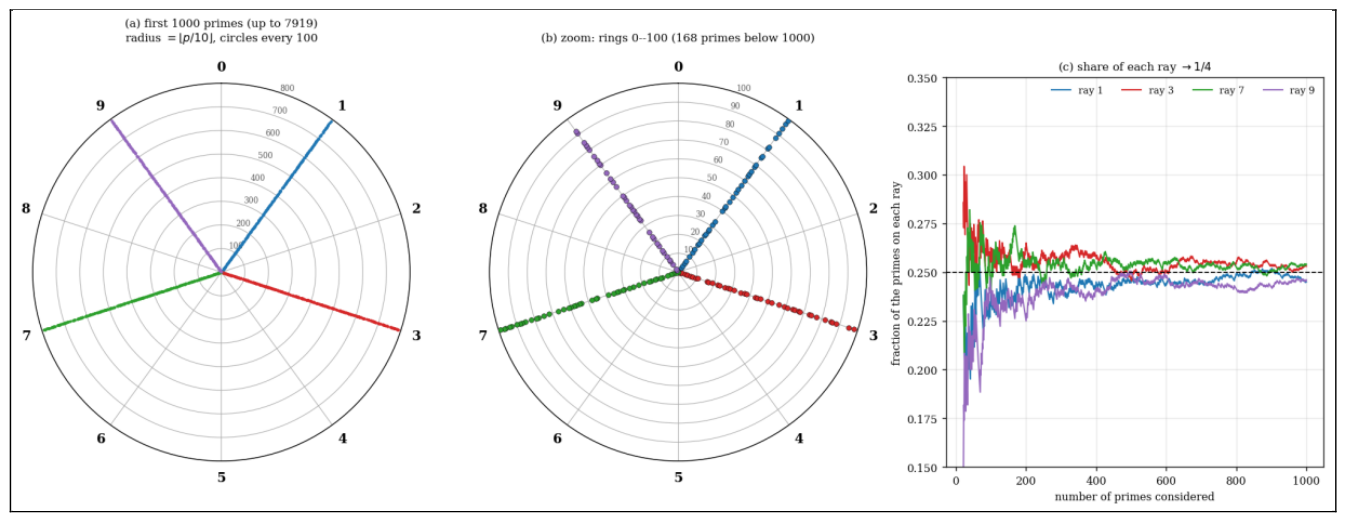
Proposition 3.4 (Rays among the first primes). [Comp. Verified, first 100, 500 and 1000 primes] Among the first 100, 500 and 1000 primes the numbers lying in the rays 1,3,7,9 are 24,26,24,24; 123,123,127,125; and 245,253,254,246 respectively; the remaining primes are 2 and 5. Among the first 1000 primes the largest deviation of a ray count from 250 is 5, and among the 168 primes below 1000 the counts are 40,42,46,38 (Table 1). For the first 1000 primes (largest prime 7919, ring 791) the mean number of rings between two consecutive primes of the same ray is 3.23, 3.13, 3.12, 3.22 for the rays 1,3,7,9.
Remark 3.5. [Honest Caveat]Figure 1 and Figure 2 illustrate the classification of Proposition 3.1 and the equidistribution of Proposition 3.2; they exhibit no phenomenon beyond those two classical facts. The slight excess of the rays 3 and 7 among the first 1000 primes (about 3 to 4 primes out of 250) is of the size of the fluctuations in Figure 2(c) and is not claimed to be systematic; at X = 108 the four counts differ from π(X)/4 by at most 0.013%.

| X | π(X) | ray 1 | ray 3 | ray 7 | ray 9 |
| 103 | 168 | 40 | 42 | 46 | 38 |
| 104 | 1,229 | 306 | 310 | 308 | 303 |
| 105 | 9,592 | 2,387 | 2,402 | 2,411 | 2,390 |
| 106 | 78,498 | 19,617 | 19,665 | 19,621 | 19,593 |
| 107 | 664,579 | 166,104 | 166,230 | 166,211 | 166,032 |
| 108 | 5,761,455 | 1,440,298 | 1,440,474 | 1,440,495 | 1,440,186 |
4. A Transfer Principle and Almost-All Theorems
Lemma 4.1 (Anchoring). [Proved] For every n ≥ 2: (i) Nn is even; (ii) Nn+1 − Nn = pn+2 − pn > 0, so n ↦ Nn is strictly increasing and injective; (iii) Nn < 3pn. More generally, for fixed k ≥ 1 and Nn,k:=pn + pn+k: Nn,k is even for n ≥ 2, strictly increasing in n, and Nn,k < (1 + 2k)pn.
Proof. For n ≥ 2 both primes are odd, giving (i). For (ii), Nn+1 − Nn = pn+2 − pn > 0. For (iii), Bertrand’s postulate [5] gives pn+1 < 2pn, so gn < pn and Nn = 2pn + gn < 3pn. Iterating, pn+k < 2kpn and hence Nn,k < (1 + 2k)pn; parity and monotonicity are as before.
Theorem 4.2 (Transfer principle). [Proved] Let q,a be as in the definition. Let 𝒜 be a set, s:𝒜 → [1,∞) a “size” function and f:𝒜 → 2ℕ a map such that, for some constants m ≥ 1, κ ≥ 1 and λ ≥ 0, #f−1(N) ≤ m for every N and f(n) ≤ κ s(n) + λ for every n ∈ 𝒜. Then for all X ≥ 1 #{n ∈ 𝒜: s(n) ≤ X, Ra,q(f(n)) = 0} ≤ m⋅#a,q(κX + λ) (4)
The inequality holds for every q ≥ 1 and every a with gcd(a,q) = 1, and the constants do not depend on any residue class of the elements of 𝒜.
Proof. Let F(X) be the set on the left. For n ∈ F(X), f(n) is even, satisfies f(n) ≤ κX + λ and Ra,q(f(n)) = 0, so f(n) ∈ a,q(κX + λ). Each element of a,q(κX + λ) has at most m preimages, whence #F(X) ≤ m #a,q(κX + λ).
Corollary 4.3 (Consecutive primes, uniform in the ray). [Proved] For every c and every X ≥ 3, #{pn ≤ X: pn≡c (q), Ra,q(Nn) = 0} ≤ #a,q(3X), and for k ≥ 1, #{pn ≤ X: pn≡c (q), Ra,q(pn + pn+k) = 0}≤#a,q((1 + 2k)X).
Proof. Take 𝒜 = {n ≥ 2}, s(n) = pn and f(n) = Nn (respectively Nn,k), which is injective by Lemma 4.1 and satisfies f(n) < 3s(n) (respectively <(1 + 2k)s(n)). Restricting to pn≡c (q) only shrinks the counted set, so (4) applies with m = 1, λ = 0 and κ = 3 (respectively 1 + 2k).
Corollary 4.4 (Shifted primes). [Proved] For every odd integer h (positive or negative) and X ≥ 1, #{p ≤ X: p > max(|h|,2), Ra,q(p + h) = 0} ≤ #a,q(X + |h|), uniformly over the rays of p modulo q.
Proof. For an odd prime p and odd h, p + h is even and p ↦ p + h is injective; apply Theorem 4.2 with 𝒜 the set of primes p > max(|h|,2), s(p) = p, f(p) = p + h, m = 1, κ = 1, λ = |h|. Primes p ≤ max(|h|,2) are excluded so that p is odd and p + h ≥ 2.
Corollary 4.5 (Almost-all statements). [Cond. Proved (Tolev, Lemma 2.3)] Let q = 2k and gcd(a,q) = 1. For every ray c with gcd(c,q) = 1 and every A > 0, #{pn ≤ X: pn≡c (q), Ra,q(Nn) = 0}≪q,AX(logX)−A = o(π(X;q,c)), so for almost all primes pn in every ray the even integer Nn = pn + pn+1 has a restricted Goldbach representation with first summand in the class a (q). The same holds for pn + pn+k with k fixed, and for p + h with h odd fixed.
Proof. By Corollary 4.3 and Theorem 2.4, the left side is at most #a,q(3X)≪q,A3X(log3X)−A≪X(logX)−A. Taking A = 2 and using π(X;q,c)∼X/(φ(q)logX) (Proposition 3.2) gives the o-statement. The statements for pn + pn+k and p + h are identical, using Corollary 4.3 and Corollary 4.4.
Remark 4.6 (Scope and triviality). [Honest Caveat] (i) By Proposition 2.2 the conclusion for Nn is automatic when pn or pn+1 lies in the class a; only the pairs of rays (c,c') with c≢a≢c' carry content. (ii) The transfer inequality holds for every modulus q, but for a modulus with an odd prime factor the exceptional set has positive density (Section 6), so Theorem 2.4 and Corollary 4.5 are statements about q = 2k. (iii) None of this bears on the pointwise question whether Ra,q(Nn) > 0 for all large n; an infinite subsequence of exceptional n of density zero is not excluded.
Remark 4.7 (Gap bound of Baker–Harman–Pintz). [Proved] Sincefor large n [2], for every ε > 0 one has Nn < (2 + ε)pn for n ≥ n0(ε); the constant κ = 3 in Corollary 4.3 may then be replaced by 2 + ε for large X, with n0(ε) not asserted to be effective. Since log((2 + ε)X) = logX + O(1), this changes the conclusion of Corollary 4.5 only by a bounded factor, and the elementary constant 3 suffices.
5. Computational Verification
Proposition 5.1 (Anchoring inequalities). [Comp. Verified, sieve; zero exceptions] Over all 216,814 pairs of consecutive primes with pn ≥ 3 and pn+1 ≤ 3 × 10⁶, and over all 5,761,453 such pairs with pn+1 ≤ 108: Nn+1 − Nn > 0 (minimum increment 4), Nn/pn < 3 (maximum ratio 8/3, attained at the smallest admissible n), and Nn is even.
Proposition 5.2 (Brute-force check for q = 8, a = 1). [Comp. Verified, R computed by convolution in double precision; range n ≤ 5000] Table 2 lists, for the first K primes, the number of n ∈ [2,K] for which Nn has no representation Nn = p1 + p2 with p1≡1 (8). The exceptional values are the same at every K: Nn ∈ {8,12,18,42,68}; no new exception occurs as K grows by a factor 100. None of the exceptions has pn≡1 or pn+1≡1 (8), in accordance with Proposition 2.2.
Representability of Nn with p1≡1 (8); first K primes (n = 2,…,K).
| K | pairsn | representable | exceptions | fraction |
| 50 | 49 | 44 | 5 | 10.20% |
| 100 | 99 | 94 | 5 | 5.05% |
| 500 | 499 | 494 | 5 | 1.00% |
| 2000 | 1999 | 1994 | 5 | 0.25% |
| 5000 | 4999 | 4994 | 5 | 0.10% |
Proposition 5.3 (Shifted primes, q = 8, a = 1). [Comp. Verified, all primes 11 ≤ p ≤ 6 × 10⁶ − 20 (412,844 primes); R1,8(N) by double-precision FFT for N ≤ 6 × 10⁶; every nonzero value is at least log17 log2 > 1.9, so values below 1 are exact zeros] For each shift h in Table 3, the number of primes p with R1,8(p + h) = 0 is small and the largest exceptional value of p + h is at most 458; no exception occurs above 458 in the range.
Primes p with R1,8(p + h) = 0, 11 ≤ p ≤ 6 × 10⁶ − 20.
| h | exceptions | largest exceptional p + h |
| −3 | 12 | 458 |
| −1 | 6 | 66 |
| 1 | 12 | 458 |
| 3 | 10 | 362 |
| 5 | 4 | 66 |
| 7 | 9 | 218 |
| 9 | 13 | 458 |
Remark 5.4.[Honest Caveat] Corollary 4.5 is asymptotic; its numerical onset depends on the explicit constants in Lemma 2.3, which are not tracked here, and need not lie in the tested range. The verification above tests only the finite ranges stated.
6. Moduli with an Odd Prime Factor Along Nn
Theorem 6.1 (Obstruction along consecutive primes). [Proved] (for the obstruction at a single N see also [1]) Let q have an odd prime factor 𝓁, gcd(a,q) = 1, and let n ≥ 2 with pn,pn+1 ≠ 𝓁. Write c≡pn and c'≡pn+1 modulo 𝓁. If c + c'≡a (𝓁), then every representation counted by Ra,q(Nn) has p2 = 𝓁, so that and in particular Ra,q(Nn) = Oq(logNn).
Proof. Suppose Nn = p1 + p2 with p1≡a (q). Then p1≡a (𝓁) and Nn≡c + c'≡a (𝓁), hence p2 = Nn − p1≡0 (𝓁). As p2 is prime, p2 = 𝓁 and p1 = Nn − 𝓁.
Corollary 6.2 (The obstructed set is infinite for 𝓵 = 3). [Proved] Let q = 3, a = 1. Then Nn≡1 (3) if and only if pn≡pn+1≡2 (3), and there are infinitely many such n. Consequently Ra,q(Nn) = O(logNn) for infinitely many n, and no asymptotic Ra,q(Nn)≍Nn/φ(q) can hold along Nn.
Proof. For pn,pn+1 > 3 the residues are 1 or 2 modulo 3, and c + c'≡1 (3) only for c = c' = 2. Infinitely many pairs of consecutive primes lie in the class 2 modulo 3 by Shiu’s theorem [10]. Apply Theorem 6.1.
Proposition 6.3 (Exact description for q = 3, a = 1). [Comp. Verified, all 216,813 pairs pn > 3, Nn ≤ 6 × 10⁶; zero exceptions] Ra,q(Nn) = 0 holds if and only if Nn≡1 (3) and Nn − 3 is composite. In particular no n outside the class pn≡pn+1≡2 (3) has Ra,q(Nn) = 0 (0 of 170,691 indices), and the predicted characterisation has 0 mismatches. Table 4 gives the fractions of obstructed indices and of exceptional indices in four ranges of Nn; over all even N ≤ 6 × 10⁶ (range 103 ≤ N) the fraction with R1,3(N) = 0 is 0.2646, and one third of even integers satisfy N≡1 (3).
q = 3, a = 1: fraction of n with Nn≡1 (3) and with R1,3(Nn) = 0.
| range of Nn | Nn≡1 (3) | R1,3(Nn) = 0 |
| [104,105) | 0.2070 | 0.1496 |
| [105,106) | 0.2069 | 0.1608 |
| [106,3 × 10⁶) | 0.2127 | 0.1700 |
| [3 × 106,6 × 106) | 0.2152 | 0.1739 |
Remark 6.4. [Honest Caveat] Along Nn the obstructed fraction is the joint frequency of the diagonal pair of rays (2,2) modulo 3, which by the Lemke Oliver–Soundararajan bias is suppressed below 1/4 and, conditionally on the Hardy–Littlewood conjecture, tends to 1/4 slowly [6]; it is not the density 1/3 that the obstruction assigns to a generic even integer. The values in Table 4 rise from about 0.207 to 0.215 over the tested ranges, which is in this direction. The infinitude in Corollary 6.2 is proved; the density is not.
Figure 3.
Obstruction along consecutive primes for q = 3, a = 1. What is plotted: the fraction of n with Nn≡1 (3) and with R1,3(Nn) = 0, in logarithmic windows of Nn up to 6 × 10⁶, against the values 1/3 (generic even integers) and 1/4 (independent rays). What it shows: the obstructed fraction stays well below 1/3 and rises slowly towards 1/4. Connection to paper: Proposition 6.3, Table 4 and Remark 6.4.
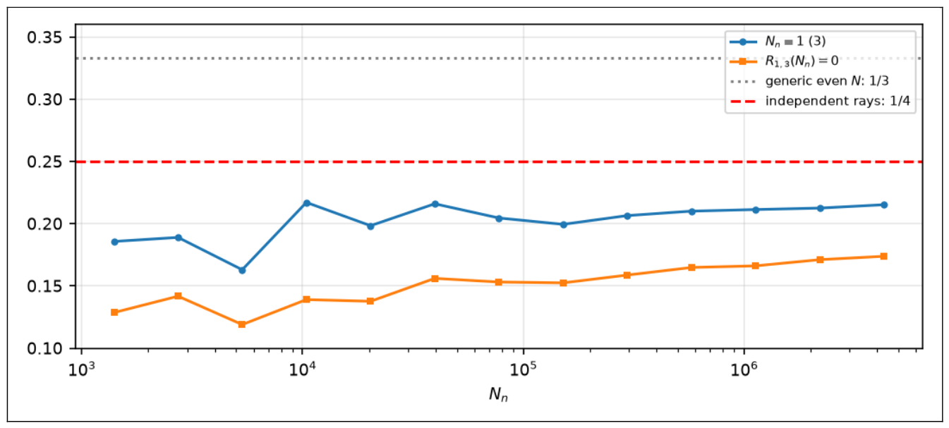
Proposition 6.5 (The case 𝓵 = 5). [Comp. Verified, all 216,812 pairs of consecutive primes pn > 5 with Nn ≤ 6 × 10⁶] For q = 5 and a = 1,2,3,4, the fraction of n with Nn≡a (5) is 0.1735, 0.1885, 0.1865, 0.1733 and the fraction with Ra,5(Nn) = 0 is 0.1358, 0.1507, 0.1504, 0.1361. The prediction of Theorem 6.1, namely Ra,5(Nn) = 0 if and only if Nn≡a (5) and Nn − 5 is not prime, has exactly three failures in the range, all with Ra,5(Nn) = 0 although Nn≢a (5): Nn = 152 = 73 + 79 for a = 1, and Nn = 18 = 7 + 11 and Nn = 68 = 31 + 37 for a = 4. The fraction of obstructed indices is below the independent-rays value 1/4 for every a.
Remark 6.6. [Honest Caveat] Theorem 6.1 proves only that Nn≡a (𝓁) forces Ra,q(Nn) ∈ {0,(log(Nn − 𝓁))log𝓁}; the converse (non-obstructed Nn have Ra,q(Nn) > 0) is not proved, and the three exceptions above are small values at which it fails for 𝓁 = 5. For 𝓁 = 3 no failure was found in the tested range (Proposition 6.3).
7. Digit Repulsion, Gaps and Admissibility
7.1. The Transition Matrix
For n = 10 and a prime p > 5 write ray(p) = p mod 10 ∈ {1,3,7,9}.
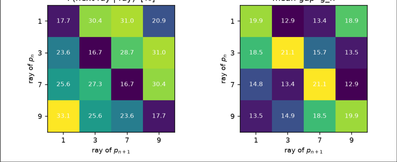
Proposition 7.1 (Digit repulsion). [Comp. Verified, all 5,761,451 pairs of consecutive primes >5 and ≤108] Table 5 gives the conditional transition matrix. The diagonal is suppressed to between 16.7% and 17.7% against 25% under independence, and every off-diagonal entry exceeds 20.8%; the qualitative bias reported in [6] is reproduced at 5.76 times the scale of the original data set.
ℙ(ray(pn+1) = b∣ray(pn) = a), pairs below 108.
| a∖b | 1 | 3 | 7 | 9 |
| 1 | 17.70% | 30.39% | 31.03% | 20.87% |
| 3 | 23.64% | 16.67% | 28.69% | 31.01% |
| 7 | 25.58% | 27.32% | 16.68% | 30.42% |
| 9 | 33.08% | 25.62% | 23.62% | 17.68% |
Proposition 7.2 (Decay with lag). [Comp. Verified, same 5,761,451 primes] The probability that ray(pn+𝓁) = ray(pn) equals 17.18, 23.28, 24.50, 24.38, 24.40, 24.48, 24.58, 24.63 (%) for 𝓁 = 1,…,8.
7.2. Mean Gap by Ray of Origin
Proposition 7.3 (Gap by ray). [Comp. Verified, all pairs with pn > 5 and pn+1 ≤ 2 × 10⁷ (1,270,603 pairs)] The global mean gap is 15.741. Conditioned on ray(pn) = 1,3,7,9 the mean gap is 15.474, 16.523, 14.836, 16.129, with deviations z = −11.5, +33.2, −38.4, +16.6 standard errors of the per-ray sample mean; the counts per ray are 317,587, 317,743, 317,690 and 317,583.
Remark 7.4 (Mechanical origin). [Comp. Verified]Table 6 conditions the mean gap on the pair (ray of pn, ray of pn+1). The diagonal entries (19.88 to 21.10) exceed every off-diagonal entry (12.86 to 18.90). The reason is elementary: a return to the same ray forces gn≡0 (10), and the smallest such gap is 10, whereas a change of ray admits gaps 2,4,6,8. Averaging the rows of Table 6 against the empirical transition frequencies of Table 5 reproduces the per-ray means of Proposition 7.3 (law of total expectation). The dependence of the mean gap on the ray of pn is therefore a corollary of the transition bias and the divisibility constraint, and is not an independent phenomenon.
Mean gap gn by (ray of pn, ray of pn+1), pn+1 ≤ 2 × 10⁷.
| a∖b | 1 | 3 | 7 | 9 |
| 1 | 19.89 | 12.86 | 13.43 | 18.90 |
| 3 | 18.52 | 21.10 | 15.72 | 13.47 |
| 7 | 14.85 | 13.40 | 21.08 | 12.88 |
| 9 | 13.50 | 14.91 | 18.50 | 19.88 |
Figure 4.
Transition and gap by pair of rays. What is plotted: left, the probability that the next prime lies in ray b given that the current prime lies in ray a (modulo 10, primes up to 108); right, the mean gap gn for each pair of rays (primes up to 2 × 10⁷). What it shows: the diagonal is suppressed on the left and enhanced on the right. Connection to paper:Table 5 and Table 6; the elementary reason for the right panel is Remark 7.4.
Proposition 7.5 (Repetition of the ray by size of the gap). [Comp. Verified, all consecutive primes 5 < pn < pn+1 ≤ 108] By Proposition 9.1, ρn+1 = ρn if and only if 10∣gn. Table 7 gives, for six classes of gap size, the share of all gaps in the class and the proportion of those gaps that return to the same ray. The gaps 2,4,6,8 make up 34.4% of all gaps and none of them can return; overall 17.18% of the gaps are multiples of 10 (the value 17.18% of Proposition 7.2 at lag 1), against 20% if the five even residues of gn modulo 10 were equally likely. Among the gaps of size at least 20 the proportion returning to the same ray is between 23% and 37% in every class, above 20%.
Gaps by size: share of all gaps and proportion keeping the ray, primes 5 < pn < pn+1 ≤ 108.
| Gap gn | share of all gaps (%) | keeping the ray (%) |
| 2–8 | 34.43 | 0.00 |
| 10–18 | 32.32 | 23.09 |
| 20–38 | 24.54 | 30.12 |
| 40–58 | 6.50 | 23.58 |
| 60–98 | 2.10 | 36.28 |
| ≥100 | 0.12 | 28.29 |
Figure 5.
Large gaps on the ray diagram. What is plotted: (a) the primes among the first 1000 with gn ≥ 20 (51 primes), each with an arrow to pn+1 coloured by the ray of pn+1; thick arrows return to the same ray (18 of the 51); the other primes are grey points; (b) the share of all gaps of each size class and the proportion of those gaps that keep the ray (
Table 7
). What it shows: the short gaps cannot return and the large gaps return in a proportion above 20%. Connection to paper: Proposition 7.5 and Remark 7.4.
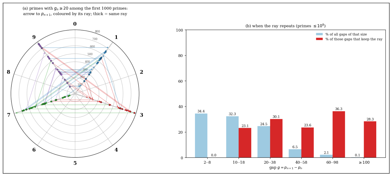
Remark 7.6. [Honest Caveat] Proposition 7.5 displays the arithmetic part of the repulsion: more than a third of all gaps are too short to return to the ray. It does not prove that this accounts for the whole bias, nor does it replace the mechanism of Lemke Oliver and Soundararajan [6], which concerns the correlations of the gap sizes and is the object of Section 7’s comparison below.
7.3. Cumulative Admissibility
For a prime q0 > 2 let
be the Hardy–Littlewood admissibility function of h with the local factor at q0 removed.
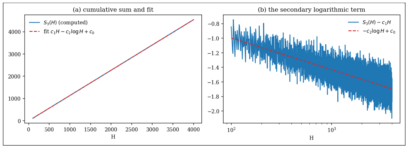
Proposition 7.7 (Cumulative sum). [Comp. Verified, least squares over every integer 100 ≤ H ≤ 4000] Fitting gives c1 = 1.136085, c2 = 0.188854, c0 = −0.127389 with R2 = 0.99999999 for q0 = 3, and c1 = 1.420105, c2 = 0.282050, c0 = −0.298717 with R2 = 0.99999996 for q0 = 5; in both cases c2 > 0, i.e., the secondary term has the sign opposite to that extrapolated from the main term.
Proposition 7.8 (Dirichlet series ofand closed forms of the constants). [Proved] For ℜs > 1, where converges absolutely, is holomorphic in ℜs > −1/2 and positive for real s > −1/2. Hence D extends meromorphically to ℜs > −1/2 with exactly two poles, both simple, at s = 1 and at s = 0. [Comp. Verified] With and , evaluated with the products taken over all primes ≤108, one finds , for q0 = 3 and , for q0 = 5; and, for q0 = 3,5 and s = 3, the series D(s) and the product agree to 8 digits.
Proof. The function depends only on the set of odd primes ≠q0 dividing h, so D(s) is an Euler product whose local factor is (1 − 2−s)−1 at p = 2, at p = q0, and, at an odd prime p ≠ q0,
because . Collecting the factors (1 − p−s)−1 gives ζ(s) times the stated product. Writing x = p−s,
so the product defining converges absolutely for ℜs > −1/2, since and converge for σ > −1/2. Each factor is positive for real s > −1, and the product equals after restoring the factors 1 − 2−1−s and and the factors (1 − p−1−s)−1 of ζ(s + 1).
Remark 7.9. [Honest Caveat] Proposition 7.8 identifies the poles of D at s = 1 and s = 0 and shows that the residue of D(s)Hs/s at the double pole s = 0 contributes , with the sign of ζ(0) = −1/2 opposite to that of the main term . It does not prove the asymptotic formula for the sharp cutoff h ≤ H: that requires control of the contour integral, which [6,13] obtain for a smooth weight. Numerically agrees with the fitted c1 in all printed digits and is within 0.3% (q0 = 3) and 0.7% (q0 = 5) of the fitted c2 of Proposition 7.7, a difference compatible with the O(1) remainder.
Figure 6.
Cumulative admissibility sum for q0 = 3. What is plotted: (a) computed directly for H ≤ 4000 and the least-squares fit c1H − c2logH + c0 over 100 ≤ H ≤ 4000; (b) the same data after subtracting c1H, on a logarithmic H-axis, against −c2logH + c0. What it shows: the curves in (a) are indistinguishable at this scale, and (b) isolates the secondary term, with c2 > 0. Connection to paper: Proposition 7.7.
Remark 7.10 (Role in the bias). [Honest Caveat] Proposition 7.7 is a numerical fit. The mechanism of Lemke Oliver and Soundararajan [6] derives the transition probabilities from such secondary terms under the Hardy–Littlewood prime tuples conjecture, so the transition formulas are conditional and are not asserted here as theorems. For q0 = 3 the two-ray transition matrix (joint probabilities, diagonal/off-diagonal) was recomputed at four scales (Table 8) and moves monotonically towards 25% in every cell as N grows.
Joint frequency of (pn mod 3, pn+1 mod 3) for consecutive primes 3 < pn < pn+1 ≤ N.
| N | pairs | (1,1) | (1,2) = (2,1) | (2,2) |
| 3 × 10⁶ | 216,813 | 21.21% | 28.76% | 21.27% |
| 107 | 664,576 | 21.50% | 28.48% | 21.53% |
| 108 | 5,761,452 | 21.94% | 28.06% | 21.95% |
| 109 | 50,847,531 | 22.25% | 27.74% | 22.26% |
Proposition 7.11 (Comparison with the Lemke Oliver–Soundararajan prediction, q0 = 3). [Comp. Verified, primes 3 < pn < pn+1 ≤ N for N = 3 × 10⁶, 107, 108, 109; the scale 109 uses a segmented sieve] Let d(N) = 1/8 loglogN/logN and let the prediction be the joint frequency 1/4 − d(N) for the cells (1,1) and (2,2) and 1/4 + d(N) for the cells (1,2) and (2,1). Table 9 gives the mean absolute error of the four observed joint frequencies against this prediction and against the value ¼. The error against the prediction is smaller than the error against ¼ at every N, by the factors 0.397, 0.381, 0.353, 0.334, and both errors decrease with N.
Mod-3 joint frequencies against the prediction 1/4∓d(N); errors in percentage points.
| N | predicted diag. | predicted off-diag. | error vs. pred. | error vs. 25% | ratio |
| 3 × 10⁶ | 22.74% | 27.26% | 1.4935 | 3.7584 | 0.397 |
| 107 | 22.84% | 27.16% | 1.3259 | 3.4818 | 0.381 |
| 108 | 23.02% | 26.98% | 1.0796 | 3.0566 | 0.353 |
| 109 | 23.17% | 26.83% | 0.9158 | 2.7442 | 0.334 |
Figure 7.
Mod-3 joint frequencies of consecutive primes against the prediction. What is plotted: left, the mean absolute error against the prediction of Proposition 7.11 and against 25% at four scales; right, observed and predicted joint frequencies at N = 108. What it shows: the prediction reproduces the suppressed diagonal and the inflated off-diagonal, with an error smaller by a factor of about 0.33 to 0.40. Connection to paper: Proposition 7.11 and Remark 7.12.
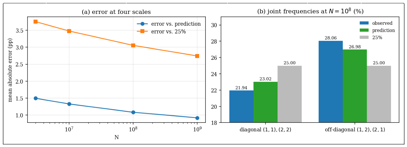
Remark 7.12. [Honest Caveat] The prediction is the leading secondary term of the argument of Lemke Oliver and Soundararajan as presented by Tao [13], and it is derived under the Hardy–Littlewood prime tuples conjecture; it is not a theorem. The agreement in Proposition 7.11 is with the leading term only, and a residual of about 1 percentage point remains at N = 108, which the formula does not describe.
8. The Second Moment Modulo q
Let q = 2k, Da,q(N):=(Ra,q(N) − Ma,q(N))/Ma,q(N) and write b≡N (mod q).
8.1. A Symmetry
Proposition 8.1 (Symmetry of the restricted sum). [Proved] For classes a,a'modulo q let. Then. In particular, for N≡2a (q) the representations counted by Ra,q(N) are closed under (p1,p2) ↦ (p2,p1), and whereas for N≢2a (q) each unordered pair {p,p'} with p≡a, p'≡N − a≢a is counted exactly once.
Proof. Exchange p1,p2 in the defining sum. If N≡2a then p1≡a implies p2 = N − p1≡a, so both orders are counted; the term p1 = p2 = N/2 is counted once. If N≢2a, the class of p2 differs from that of p1, and only one order of an unordered pair is counted.
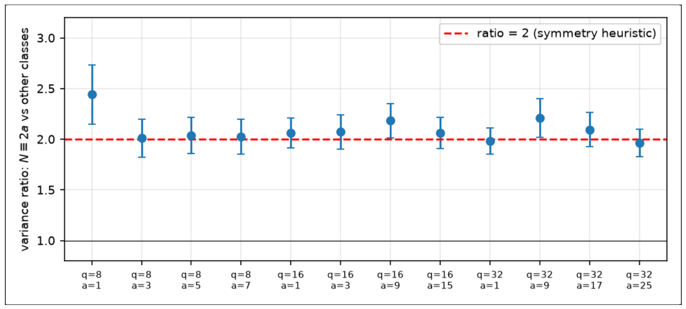
Remark 8.2 (Heuristic consequence). [Honest Caveat] If the unordered pair counts fluctuated like independent Poisson variables with the same mean μ, the doubling in Proposition 8.1 would multiply the variance of Ra,q(N) by 4 ⋅ (μ/2)/μ = 2 when N≡2a (q). This is a heuristic explanation of the numerical ratio below, not a proof.
Proposition 8.3 (Second moment by class of N, q = 8). [Comp. Verified; Ra,8(N) computed by FFT convolution of the weighted prime indicators for all even N ≤ 6 × 10⁶, Ma,8 from an exact factorisation sieve] (i) For a = 1 and even N ∈ [105,6 × 10⁶], the mean of (in units of 10−5) is 9.70, 24.21, 9.76, 9.29 for N≡0,2,4,6 (8), and the mean of D1,8 (in units of 10−3) is −2.991, −5.715, −2.920, −2.999. (ii) For even N ∈ [106,6 × 10⁶], let ρa,q be the mean of on N≡2a (q) divided by its mean on the other classes. For q = 8, a = 1,3,5,7: ρ = 2.44, 2.01, 2.04, 2.03; for q = 16 and all eight a: 2.06, 2.07, 2.04, 2.00, 2.18, 2.08, 2.08, 2.06 (mean 2.07); for q = 32 and all sixteen a the mean is 2.04 and the range 1.94 to 2.21. Delete-one jackknife standard errors over 20 interleaved blocks are 0.17 to 0.29 for q = 8 and 0.13 to 0.19 for the values of a tested at q = 16,32 (Figure 8); every value is within 1.6 standard errors of 2, including ρ1,8 = 2.44 ± 0.29.
Figure 8.
Variance ratio on the class N≡2a (q). What is plotted: the ratio ρa,qof the mean ofon N≡2a (q) to its mean on the other classes, for selected (q,a), with jackknife error bars, against the value 2. What it shows: every value lies within 1.6 standard errors of 2. Connection to paper: Proposition 8.3 and Remark 8.2.
Proposition 8.4 (Size of the second moment). [Comp. Verified; q = 8, a = 1, all even N ≤ X, X ≤ 6 × 10⁶] Table 10 gives relative to X3 and to X3/logX. The second ratio decreases monotonically in X, from 4.68 × 10⁻⁴ at X = 2 × 10⁵ to 3.19 × 10⁻⁵ at X = 6 × 10⁶.
Second moment of the error, q = 8, a = 1.
| X | ||
| 2 × 10⁵ | 3.84 × 10⁻⁵ | 4.68 × 10⁻⁴ |
| 5 × 10⁵ | 1.83 × 10⁻⁵ | 2.41 × 10⁻⁴ |
| 106 | 1.00 × 10⁻⁵ | 1.39 × 10⁻⁴ |
| 2 × 10⁶ | 5.65 × 10⁻⁶ | 8.20 × 10⁻⁵ |
| 3 × 10⁶ | 4.00 × 10⁻⁶ | 5.97 × 10⁻⁵ |
| 4.5 × 10⁶ | 2.67 × 10⁻⁶ | 4.09 × 10⁻⁵ |
| 6 × 10⁶ | 2.05 × 10⁻⁶ | 3.19 × 10⁻⁵ |
Figure 9.
Second moment of the error for q = 8, a = 1. What is plotted: left, on logarithmic axes with the line ∝X−1; right, the same sum divided by X3/logX. What it shows: between X = 2 × 10⁵ and X = 6 × 10⁶ the left curve falls by a factor 18.8, a local exponent of about −0.86, slightly slower than X−1; the right curve decreases monotonically. Connection to paper: Proposition 8.4 and Remark 8.5.
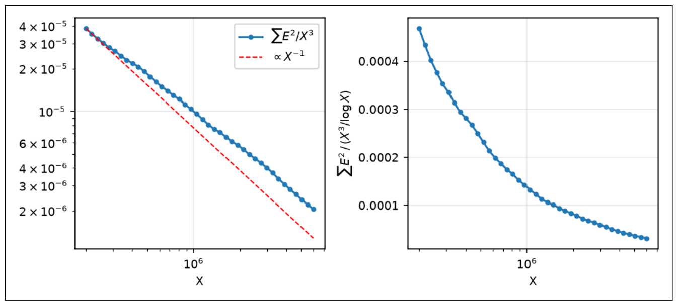
Remark 8.5. [Honest Caveat] Proposition 8.4 is a finite-range measurement. It is compatible with a much smaller order than X3/logX, but it proves nothing about the limit, and the range X ≤ 6 × 10⁶ is far from any regime where a lower-order term such as X3/logX could be excluded or confirmed. For q = 1 the mean square of the Goldbach error is known to be ≪X3(logX)−A for every A > 0 [12], which is compatible with the decrease seen in Table 10 and incompatible with a lower bound of order X3/logX; the analogous statement for q = 2k is not proved here.
8.2. From the Ray of pn to the Class of Nn
Since Nn≡c + c' (q) with c,c' the rays of pn,pn+1, the distribution of Nn mod q given c is read off the transition matrix of consecutive primes modulo q.
Proposition 8.6 (Class of Nn given the ray, q = 8). [Comp. Verified, all 216,811 pairs of consecutive primes >7 with Nn ≤ 6 × 10⁶] Table 11 gives ℙ(Nn≡b (8)∣pn≡c (8)). For rays c = 1,5 the class b = 2 has probability 0.166 and 0.163, and for rays c = 3,7 it has probability 0.268 and 0.267: the classes b≡2 (8) arise from the pairs (1,1),(5,5),(3,7),(7,3), and the two diagonal pairs are suppressed by the digit-repulsion bias.
ℙ(Nn≡b (8)∣pn≡c (8)), Nn ≤ 6 × 10⁶.
| c∖b | 0 | 2 | 4 | 6 |
| 1 | 0.2838 | 0.1664 | 0.2842 | 0.2656 |
| 3 | 0.2868 | 0.2677 | 0.2799 | 0.1657 |
| 5 | 0.2846 | 0.1630 | 0.2863 | 0.2662 |
| 7 | 0.2849 | 0.2667 | 0.2848 | 0.1637 |
Proposition 8.7 (Second moment along Nn by ray, q = 8, a = 1). [Comp. Verified; 211,683 pairs of consecutive primes >7 with 105 ≤ Nn ≤ 6 × 10⁶; jackknife over 20 interleaved blocks n mod 20] Put D = D1,8(Nn) and let be the mean of D2 over pn≡c (8), in units of 10−5. Then for c = 1,3,5,7, and the mean over all n is 10.79. The pairwise differences are: rays 1 − 3: −1.39 ± 0.18 (z = −7.8); 1 − 7: −1.70 ± 0.25 (z = −6.9); 5 − 3: −1.49 ± 0.19 (z = −8.0); 5 − 7: −1.80 ± 0.19 (z = −9.3); 1 − 5: +0.10 ± 0.16; 3 − 7: −0.31 ± 0.24. The second moment along Nn therefore depends on the ray of pn: rays 3 and 7 exceed rays 1 and 5.
Proposition 8.8 (Prediction by the class of Nn). [Comp. Verified; same sample] Letbe the mean ofover all even N ∈ [105,6 × 10⁶] in the same cell, where a cell is a logarithmic window of N (15 windows) together with the class of N modulo 8 (respectively modulo 8, 3 and 5). Then, in units of 10−5: (i) windows alone predict the overall mean as 14.22; (ii) adding the class modulo 8 gives 13.66, and predicts the ray differences 1 − 3, 1 − 7, 5 − 3, 5 − 7, 1 − 5, 3 − 7 as −1.68, −1.66, −1.75, −1.73, +0.07, +0.02; (iii) adding the classes modulo 3 and 5 gives 11.05 for the overall mean (observed 10.79), the per-ray means 10.36, 11.72, 10.34, 11.78 (observed 10.04, 11.43, 9.94, 11.74), and the ray differences −1.36, −1.41, −1.38, −1.43, +0.02, −0.05, against the observed values of Proposition 8.7. The differences observed minus predicted in (iii) for rays 1,3,5,7 are −0.32 ± 0.12, −0.29 ± 0.14, −0.41 ± 0.07 and −0.04 ± 0.15.
Figure 10.
Second moment along Nn by ray, q = 8. What is plotted: the observed mean of D1,8(Nn)2 by ray of pn modulo 8, and its prediction from windows of N combined with the class of N modulo 8, and modulo 8,3,5. What it shows: rays 3 and 7 exceed rays 1 and 5, and the prediction reproduces the ordering and the size of the differences. Connection to paper: Propositions 8.7 and 8.8 and Remark 8.9.
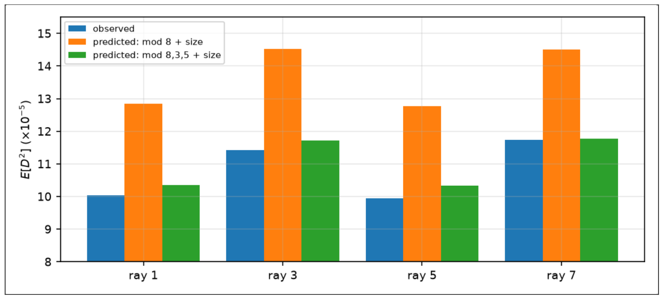
Remark 8.9 (Interpretation). [Honest Caveat] The ray of pn acts on the second moment through the class of Nn: the transition matrix of Proposition 8.6 sends more mass to Nn≡2 (8) from rays 3,7, and that class has twice the variance (Proposition 8.3). The ordering and size of the differences are predicted by the class modulo 8 alone to about 20% (−1.7 against observed −1.4 to −1.8). The inclusion of the classes modulo 3 and 5 was decided after seeing that windows and the class modulo 8 over-predict the level; at q = 8 it is therefore a fit choice and not a pre-specified prediction; Proposition 8.10 applies the same recipe, unchanged, at q = 16. The remaining discrepancy (−0.3 × 10⁻⁵ for rays 1,3,5, two to four standard errors) is about 3% of the level and is not explained. The sample is restricted to Nn ≥ 105 and is compared with a reference population in the same range of N, because D2 is larger by an order of magnitude at small N.
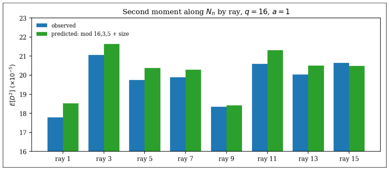
Proposition 8.10 (Prediction fixed in advance, q = 16, a = 1). [Comp. Verified; 211,683 pairs of consecutive primes >7 with 105 ≤ Nn ≤ 6 × 10⁶; jackknife over 20 interleaved blocks] The recipe of Proposition 8.8(iii) was applied unchanged with the class modulo 8 replaced by the class of N modulo 16: cells are 15 logarithmic windows of N together with the classes of N modulo 16, 3 and 5, and the prediction for Nn is the mean of over all even N ∈ [105,6 × 10⁶] in the same cell. Then, in units of 10−5: the overall mean is observed 19.77 and predicted 20.19; the means over the eight rays c = 1,3,5,7,9,11,13,15 of pn modulo 16 are observed 17.79, 21.07, 19.75, 19.90, 18.34, 20.59, 20.03, 20.64 and predicted 18.52, 21.64, 20.37, 20.29, 18.42, 21.31, 20.50, 20.48. The spread between the largest and smallest ray mean is 3.28 observed and 3.22 predicted, and the correlation between observed and predicted ray means is 0.962. The differences of the ray means against ray 1 (rays 3,5,7,9,11,13,15) are observed +3.28, +1.96, +2.10, +0.55, +2.80, +2.24, +2.85 (z = +6.1, +4.6, +3.6, +1.0, +4.6, +3.5, +4.2) and predicted +3.12, +1.84, +1.77, −0.10, +2.79, +1.98, +1.95. The differences observed minus predicted for the eight ray means range from −0.73 to +0.16, with standard errors 0.20 to 0.39; the largest in absolute z is ray 5 (−0.61 ± 0.20, z = −3.1).
Figure 11.
Second moment along Nn by ray, q = 16. What is plotted: the observed mean of D1,16(Nn)2 by ray of pn modulo 16 and its prediction from the classes of N modulo 16, 3 and 5 combined with windows of N. What it shows: the recipe fixed in advance reproduces the level and the pattern among the eight rays. Connection to paper: Proposition 8.10 and Remark 8.13.
Proposition 8.11 (The same recipe at other pairs (q,a)). [Comp. Verified; same sample of 211,683 pairs and same reference population; recipe of Proposition 8.10 unchanged, with the class modulo q in place of the class modulo 16] Table 12 lists, for four pairs (q,a), the overall means of along Nn (observed and predicted, in units of 10−5), the relative difference observed minus predicted with its delete-one jackknife z-value, the spread between the largest and smallest ray mean (observed and predicted), and the correlation between observed and predicted ray means over the reduced rays modulo q. In every case the observed overall mean is below the predicted one, by 2.1% to 3.0%, and the number of rays whose observed mean is below the prediction is 4/4, 7/8, 8/8 and 15/16 respectively.
Recipe of Proposition 8.10 at four pairs (q,a); means in units of 10−5.
| q | a | obs. | pred. | diff. (%) | z | spread obs./pred. | corr. |
| 8 | 1 | 10.79 | 11.05 | −2.4 | −4.0 | 1.80 / 1.43 | 0.993 |
| 16 | 1 | 19.77 | 20.19 | −2.1 | −3.5 | 3.28 / 3.22 | 0.962 |
| 16 | 9 | 19.42 | 20.02 | −3.0 | −5.1 | 1.93 / 1.87 | 0.958 |
| 32 | 1 | 38.60 | 39.53 | −2.4 | −4.1 | 6.50 / 6.81 | 0.940 |
Proposition 8.12 (Effect of further small primes, exploratory). [Comp. Verified; exploratory, the additional moduli were chosen after seeingTable 12] Adding the class of N modulo 7, and then modulo 7 and 11, to the cells of the prediction changes the relative difference observed minus predicted (with z in parentheses) from −2.4% (−4.0) to −1.6% (−2.8) and −1.3% (−2.3) at (q,a) = (8,1); from −2.1% (−3.5) to −1.0% (−1.7) and −0.6% (−1.6) at (16,1); and from −3.0% (−5.1) to −2.0% (−3.6) and −1.4% (−2.9) at (16,9).
Remark 8.13. [Honest Caveat] The prediction at q = 16 uses the recipe of q = 8 without adjustment, so it is a test and not a fit. It reproduces the ordering, the spread and the level of the second moment by ray, but it over-predicts by about 3% for most rays, and the eight differences are not independent (they share a common shift), so the z-values above must not be combined as independent evidence. The over-prediction recurs at every pair tested (Table 12) and decreases monotonically when the classes modulo 7 and 11 are added (Proposition 8.12), which is consistent with Nn = 2pn + gn differing from a generic even integer through its residues modulo small primes; this reading is exploratory, and a residual of about 1% to 1.4% remains at the pairs tested. At q = 8 the spread among rays is under-predicted (1.43 against 1.80), while at q = 32 it is over-predicted (6.81 against 6.50). All results are for one range of N, 105 ≤ N ≤ 6 × 10⁶.
9. Predicting the Next Ray and the Gap
Let ray(p) = p mod 10 for p > 5, and write ρn = ray(pn) ∈ {1,3,7,9}.
Proposition 9.1 (Ray–gap identity). [Proved] For n with pn > 5: gn≡ρn+1 − ρn (mod 10). In particular ρn+1 = ρn if and only if 10∣gn, and then gn ≥ 10; the ray of pn+1 is determined by ρn and gn mod 10, and conversely.
Proof. gn = pn+1 − pn reduces modulo 10 to ρn+1 − ρn. If ρn+1 = ρn then 10∣gn > 0.
Hence predicting the class of gn modulo 10 from the past is the same problem as predicting ρn+1.
Proposition 9.2 (Prediction out of sample). [Comp. Verified; recipe fixed before the run; all pairs (pn,pn+1) with 5 < pn < pn+1 ≤ 108 (5,761,451 pairs); temporal split: training pn ≤ 5 × 10⁷ (3,001,131 pairs), test pn > 5 × 10⁷ (2,760,320 pairs)] For the context (ρn,ρn−1,…,ρn−k+1) the predictor of ρn+1 is the most frequent next ray in the training set, and the predictor of gn/logpn is the training mean in the same context. Table 13 gives, on the test set, the accuracy for ρn+1 (baseline 0.2500, standard error 0.0003), the information gain in bits over the marginal distribution of ρn+1 (uniform: 2 bits), and the coefficient of determination R2 for gn/logpn against the training global mean. Accuracy is 0.311 with one ray and 0.316 with four, an excess of about 6.5 points over 0.25; the information gain is 0.036 bits out of 2; and R2 for the normalised gap is at most 0.0019. Adding the previous gap gn−1 in six quantile bins to three rays gives accuracy 0.328, 0.048 bits and R2 = 0.0048; the previous gap alone gives accuracy 0.259, 0.001 bits and R2 = 0.0014. The most likely next ray given ρn = 1,3,7,9 is 7,9,9,1, with test accuracy 0.3075, 0.3072, 0.3020, 0.3277.
Out-of-sample prediction of ρn+1 and gn/logpn from the last k rays modulo 10; test set pn > 5 × 10⁷.
| k | accuracy of ρn+1 | information gain (bits) | R2 of gn/logpn |
| 1 | 0.3111 | 0.0330 | 0.00164 |
| 2 | 0.3152 | 0.0356 | 0.00178 |
| 3 | 0.3158 | 0.0360 | 0.00186 |
| 4 | 0.3160 | 0.0363 | 0.00187 |
| 5 | 0.3160 | 0.0361 | 0.00165 |
| 6 | 0.3144 | 0.0340 | 0.00062 |
Proposition 9.3 (Reference level for the gap). [Comp. Verified; same split] Using the exact value of gn mod 10 (which is not available before pn+1 is known) as the context, the training means of gn/logpn by class give R2 = 0.0355 on the test set.
Remark 9.4 (Interpretation). [Honest Caveat] The rays of the past predict the ray of the next prime better than chance, and essentially all of this comes from the last ray: the gain from k = 1 to k = 4 is 0.003 bits, in line with the decay with lag in Proposition 7.2. The size of the gap is not predicted: the class of gn mod 10, even if known, would explain 3.6% of the variance of gn/logpn, and the rays of the past explain at most 0.19%, which is about a twentieth of that reference. The decrease at k = 6 reflects the 4,096 contexts estimated from the training set. The accuracy of about 31.6% is a measurement of the Lemke Oliver–Soundararajan bias as a predictor and is not a new mechanism; it is not asserted to persist at larger scales, where the bias decays. The context of one ray is fixed by the transition matrix of Table 5, whose row maxima (31.0%, 31.0%, 30.4%, 33.1% in sample) are reproduced out of sample.
10. Open Questions
Open Question 57 (Power saving for q = 2k). [Open] Prove for some Δq > 0, q = 2k, k ≥ 1 and every a, with full details for the character sums modulo q; the case q = 1 is the theorem of Montgomery and Vaughan [8]. Also give a self-contained proof of Lemma 2.3, or of Theorem 2.4 without it. A power saving would give, via Corollary 4.3, .
Open Question 58 (Explicit threshold). [Open] Give an explicit X1 = X1(q,a,c) beyond which #a,q(3X) < π(X;q,c), i.e., not merely asymptotically; this requires explicit constants in Lemma 2.3.
Open Question 59 (Density of the obstruction). [Open] For q = 3, a = 1 decide whether the natural density of {n:pn≡pn+1≡2 (3)} exists; conditionally on the Hardy–Littlewood conjecture it is 1/4 [6]. Determine the density of {n:Ra,q(Nn) = 0}, which by Proposition 6.3 equals that of {n:Nn≡1 (3)} once the primes among Nn − 3 have density zero along this set.
Open Question 60 (Class-dependent second moment). [Open] For q = 2k, determine whether (suitably normalised by the number of terms and the range) has a limit as X → ∞, and its value; Proposition 8.3 gives values between 1.94 and 2.44 at q = 8,16,32, all within 1.6 standard errors of 2.
Open Question 61 (Ray-dependent second moment). [Open] Fix q = 2k and gcd(a,q) = 1. For rays c coprime to q define and π(X;q,c)−1Wc(X). Decide whether there exist rays c0 ≠ c1 for which the limit inferior and superior of the ratio of these normalised quantities are not both 1. Propositions 8.7, 8.8 and 8.10 show a significant dependence at q = 8 and q = 16 in the range 105 ≤ Nn ≤ 6 × 10⁶, which the class of Nn predicts to about 20% at q = 8 and to about 2% in level and spread at q = 16; whether it persists as X → ∞ depends on Open Question 10.4 and on the limiting transition probabilities.
Open Question 62 (General modulus, closed form). [Open] Derive, for q with φ(q) > 2 (in particular q = 10 and q = 2k, k ≥ 3), the analogue of the two-ray transition formula for consecutive primes, and compare it with Table 5 at the same rigour as for q = 3.
Open Question 63 (Shift dependence). [Open] For fixed odd h, Corollary 4.4 bounds the primes p with R(p + h) = 0. Determine whether the rate depends on h through 𝔖(p + h), and whether the dependence is ray-independent at leading order.
11. Conclusions
The restricted Goldbach sum can be evaluated along special sequences of even integers without any new analytic input beyond the mean-value lemma of Tolev, because an injective map into the even integers with linear growth transfers every bound on the exceptional set. For consecutive primes, for the k-th next prime and for shifted primes this gives statements uniform in the ray of pn; with Theorem 2.4 they are almost-all theorems with a saving of every power of logX, and they are informative only where the obvious representation by pn and pn+1 themselves is not available.
For a modulus with an odd prime factor the same sequence exposes the local obstruction in a concrete form: the condition Nn≡a (𝓁) is a condition on the pair of rays of two consecutive primes, it holds infinitely often by Shiu’s theorem, and for q = 3 it accounts exactly for every zero of R1,3(Nn) in the tested range. The frequency of the obstructed set is governed by the bias between consecutive primes that Lemke Oliver and Soundararajan discovered, which the tables above reproduce at a larger scale.
Finally, the symmetry p1 ↔ p2 doubles the relative variance of Ra,q(N) on the class N≡2a (q), a value fixed in advance and confirmed for q = 8,16,32 within about one standard error. Since the ray of pn controls the class of Nn through the transition matrix modulo q, the second moment along Nn depends on the ray, significantly (z = 7 to 9) in the tested range, and the class of Nn predicts the size of this dependence to about 20% (modulo 8 alone) and to within about two standard errors when the classes modulo 3 and 5 are added, with the caveat of Remark 8.9; the same recipe applied unchanged at q = 16 (Proposition 8.10) reproduces the level and the pattern among rays, with a small systematic over-prediction (Table 12). The rays of the past predict the next ray with accuracy about 0.31 to 0.32 out of sample (Proposition 9.2) but not the size of the gap. The precise limiting statements are recorded as open questions.
12. Verification Methodology
Every statement labelled [Comp. Verified] was recomputed from scratch by Python scripts (numpy, scipy). Primes up to 108 come from a boolean sieve of Eratosthenes; the scale N = 109 of Table 8 and Table 9 uses a segmented sieve with the same pair-counting code. Ra,q(N) for all even N ≤ 6 × 10⁶ is obtained from one FFT convolution (scipy.signal.fftconvolve, double precision) of the log-weighted prime indicator restricted to p1≡a (q) with the unrestricted one; every nonzero value of Ra,q(N) is at least log2 ⋅ logpmin, where pmin is the least prime ≡a (q), so the zeros are unambiguous. 𝔖(N) is evaluated exactly by a multiplicative sieve, and C2 = 0.660161816… is the product over all odd primes ≤108. In Section 8, the 15 logarithmic windows of N ∈ [105,6 × 10⁶] have equally spaced logarithms. Every script first reproduced π(106) = 78,498, π(2 × 10⁶) = 148,933, π(107) = 664,579 and π(108) = 5,761,455 before being trusted, and the numbers ofTable 1, Table 5, Table 8, Table 9, Table 10, Table 11, Table 12 and Table 13 were reproduced to the printed digits.
References
- Anderson, F. Restricted Goldbach sums in arithmetic progressions: local obstructions, an explicit almost-all framework, and a general-modulus extension. Preprints.org 2026. [Google Scholar] [CrossRef]
- Baker, R. C.; Harman, G.; Pintz, J. The difference between consecutive primes, II. Proc. Lond. Math. Soc. (3) 2001, vol. 83(no. 3), 532–562. [Google Scholar] [CrossRef]
- Bauer, C. Goldbach’s conjecture in arithmetic progressions: number and size of exceptional prime moduli. Arch. Math. 2017, vol. 108(no. 2), 159–172. [Google Scholar] [CrossRef]
- Davenport, H. Multiplicative Number Theory. In Graduate Texts in Mathematics 74, 3rd ed.; Montgomery, H. L., Ed.; Springer-Verlag: New York, 2000. [Google Scholar]
- Heath-Brown, D. R.; Silverman, J. H. (Eds.) G. H. Hardy and E. M. Wright, An Introduction to the Theory of Numbers, 6th ed.; Oxford University Press: Oxford, 2008. [Google Scholar]
- Lemke Oliver, R. J.; Soundararajan, K. Unexpected biases in the distribution of consecutive primes. Proc. Natl. Acad. Sci. USA 2016, vol. 113(no. 31), E4446–E4454. [Google Scholar]
- Liu, M. C.; Zhan, T. “The Goldbach problem with primes in arithmetic progressions,” in Analytic Number Theory (Kyoto, 1996). In London Mathematical Society Lecture Note Series 247; Cambridge University Press: Cambridge, 1997; pp. 227–251. [Google Scholar]
- Montgomery, H. L.; Vaughan, R. C. The exceptional set in Goldbach’s problem. Acta Arith. 1975, vol. 27, 353–370. [Google Scholar] [CrossRef]
- Pintz, J. A new explicit formula in the additive theory of primes with applications II: the exceptional set in Goldbach’s problem. arXiv 2018, arXiv:1804.09084. [Google Scholar]
- Shiu, D. K. L. Strings of congruent primes. J. Lond. Math. Soc. (2) 2000, vol. 61(no. 2), 359–373. [Google Scholar] [CrossRef]
- Tolev, D. I. The binary Goldbach problem with arithmetic weights attached to one of the variables. Acta Arith. 2010, vol. 142(no. 2), 169–178. [Google Scholar] [CrossRef]
- R. C. Vaughan, The Hardy–Littlewood Method. In Cambridge Tracts in Mathematics 125, 2nd ed.; Cambridge University Press: Cambridge, 1997.
- Tao, T. “Biases between consecutive primes,” personal blog. 14 March 2016. Available online: https://terrytao.wordpress.com/2016/03/14/biases-between-consecutive-primes/.
Figure 1.
Base-10 ray diagram. What is plotted: each prime at angle 2π (p mod 10)/10, measured clockwise from the top, with the ten spokes labelled by the last digit; (a) the primes up to 100 at radius p (circles every 10), each labelled by its value; (b) the first 100 primes (up to 541) at radius ⌊p/10 ⌋ (circles every 10). What it shows: apart from 2 and 5, which lie on the spokes 2 and 5 at radius 2 and 5 in (a) and at the origin in (b), only the four rays 1,3,7,9 are occupied. Connection to paper: illustrates Propositions 3.1 and 3.3.
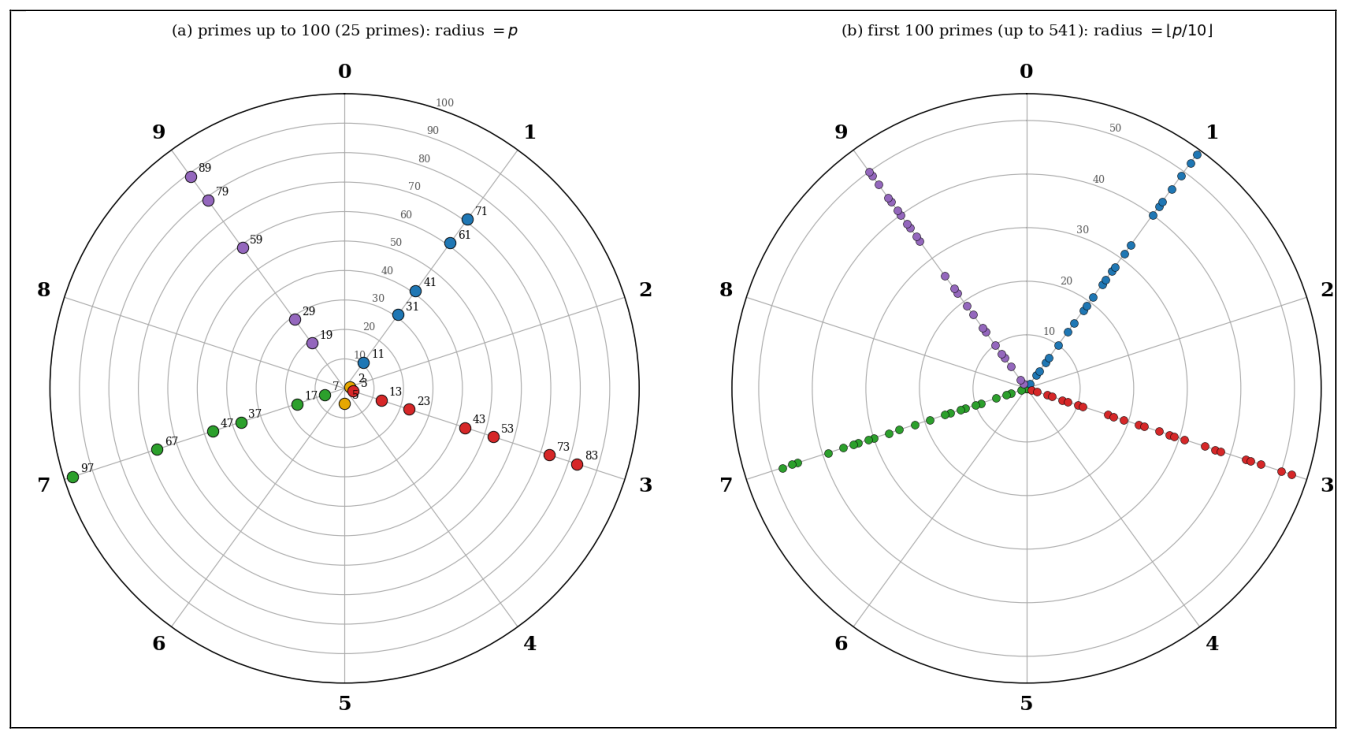
Figure 2.
Ray diagram for the first 1000 primes. What is plotted: (a) the first 1000 primes at radius ⌊p/10 ⌋, circles every 100; (b) the rings 0–100, i.e., the 168 primes below 1000; (c) the fraction of the first k primes lying on each of the rays 1,3,7,9, for k ≤ 1000, against the value 1/4. What it shows: the four rays fill in as more primes are added, the other six spokes stay empty, and the four proportions oscillate and settle near 1/4. Connection to paper: Proposition 3.4; this is Proposition 3.2 seen at small scale.
Disclaimer/Publisher’s Note: The statements, opinions and data contained in all publications are solely those of the individual author(s) and contributor(s) and not of MDPI and/or the editor(s). MDPI and/or the editor(s) disclaim responsibility for any injury to people or property resulting from any ideas, methods, instructions or products referred to in the content. |
© 2026 by the author. Licensee MDPI, Basel, Switzerland. This article is an open access article distributed under the terms and conditions of the Creative Commons Attribution (CC BY) license.
Copyright: This open access article is published under a Creative Commons CC BY 4.0 license, which permit the free download, distribution, and reuse, provided that the author and preprint are cited in any reuse.