

Submitted:
11 October 2026
Posted:
14 October 2026
You are already at the latest version
Abstract
For \(q = 2^k\) and \(\gcd(a,q)=1\) let \(R_{a,q}(N)=\sum_{p_1+p_2=N,\ p_1\equiv a\ (q)} (\log p_1)(\log p_2)\) be the restricted weighted Goldbach sum, with candidate main term \(M_{a,q}(N)=\frac{2C_2}{\varphi(q)}\,\mathfrak{S}(N)\,N\) and exceptional set \(\mathcal{E}_{a,q}(X)=\{N\le X \text{ even}: R_{a,q}(N)=0\}\). We first prove, by the circle method with the additive-shift decomposition of the sum over a progression modulo \(2^k\), an exact evaluation of the singular series of the progression and the mean-square bound \(\sum_{N\le X}\left|R_{a,q}(N)-M_{a,q}(N)\right|^{2}\ll_{A,q} X^{3}(\log X)^{-A}\) for every \(A>0\), hence \(\#\mathcal{E}_{a,q}(X)\ll_{A,q} X(\log X)^{-A}\). Writing \(p_n\) for the \(n\)-th prime, \(g_n=p_{n+1}-p_n\) and \(N_n=p_n+p_{n+1}\), we then prove an elementary transfer principle: if \(f\) maps a set of indices injectively (or with bounded multiplicity) into the even integers with at most linear growth, the number of indices $n\le X$ with \(R_{a,q}(f(n))=0\) is at most a bounded multiple of \(\#\mathcal{E}_{a,q}(\kappa X+\lambda)\). The consequences are uniform in the residue class ("ray") of \(p_n\) modulo \(q\) and cover \(N_n=p_n+p_{n+1}\), \(p_n+p_{n+k}\) and the shifted primes \(p+h\) with \(h\) odd; each of these sets of even integers has a restricted Goldbach representation for almost all primes in every ray, with a saving of every power of \(\log X\). We record which of the representations are trivial (a summand equal to \(p_n\) or \(p_{n+1}\)). For a modulus \(q\) with an odd prime factor \(\ell\) we prove that \(N_n\equiv a\ (\ell)\) is a condition on the pair of rays of \(p_n\) and \(p_{n+1}\), that \(R_{a,q}(N_n)=O(\log N_n)\) on that set, and, by a theorem of Shiu, that this set is infinite; for \(q=3\) we verify that \(R_{a,q}(N_n)=0\) if and only if \(N_n\equiv 1\ (3)\) and \(N_n-3\) is composite. The digit-repulsion bias of Lemke Oliver and Soundararajan is documented on 5,761,451 consecutive pairs below \(10^8\), together with the dependence of the mean gap on the ray of origin, a fit of the cumulative admissibility function with closed-form constants, and a comparison of the mod-3 joint frequencies with the Lemke Oliver–Soundararajan prediction at four scales up to \(10^9\). Next, the relative second moment of \(R_{a,q}(N)-M_{a,q}(N)\) depends on \(N\) modulo \(q\) through the symmetry \(p_1\leftrightarrow p_2\): for $N\equiv 2a\ (q)$ the variance ratio is 2.0 to 2.1 for \(q=16,32\) and within two standard errors of 2 for every class tested at \(q=8,16,32\). Along \(N_n\) this class effect, together with the residues of \(N_n\) modulo 3 and 5, predicts the second moment by ray of \(p_n\) to within 3% overall, and a recipe fixed in advance at \(q=16\) predicts the level, the spread among the eight rays, and the pattern across rays with correlation 0.96. In a temporal split of the primes below \(10^8\) the last ray predicts the next ray with accuracy 0.311 against 0.25, while the rays of the past explain at most 0.19% of the variance of the normalised gap. Finally, the amplitude \(\mathfrak{S}(p+h)\) of the main term along shifted primes has a limit law given by an explicit random Euler product \(Y_h\), with convergence of all moments, an entire moment generating function, a doubly exponentially thin upper tail, and no atoms. Every statement carries an explicit status label. This paper continues [18]: it restates its local-obstruction theorem and strengthens its second-moment estimate to a saving of every power of \(\log X\); Section 1.5 records the precise relation.
Keywords:
restricted Goldbach problem
; consecutive primes
; shifted primes
; almost-all theorem
; exceptional set
; mean-square estimate
; circle method
; local obstruction
; Hardy–Littlewood singular series
; Lemke Oliver–Soundararajan bias
; random Euler product
MSC: 2020 Mathematics Subject Classification: 11P32 (primary); 11N05; 11N13; 11N37; 11P55; 11K65 (secondary)
1. Introduction
1.1. Rays and Gaps in the Restricted Goldbach Programme
Fix q ≥ 1 and gcd(a,q) = 1. The restricted weighted Goldbach sum is
with candidate main term
where is the twin-prime constant. Put a,q(X):={N ≤ X, N even:Ra,q(N) = 0} and . For a prime p the residue class of p modulo n is called its ray of modulus n, and ⌊p/n⌋ is its ring. The gap to the next prime is gn = pn+1 − pn, and the even integer built from two consecutive primes is
Nn:=pn + pn+1 = 2pn + gn (n ≥ 2).
The rays of pn and pn+1 modulo q determine Nn modulo q, and the gap gn determines how far Nn is from 2pn. This paper studies four consequences: (i) the mean-square behaviour of Ra,q − Ma,q for q = 2k and the resulting exceptional-set bound with a saving of every power of logX (Section 4); (ii) an elementary transfer of almost-all statements for Ra,q to sequences of the form Nn and p + h (Section 6 and Section 7); (iii) what the local obstruction of a modulus with an odd prime factor does along Nn (Section 8); (iv) the digit-repulsion bias between consecutive primes, the dependence of the second moment of Ra,q − Ma,q on N mod q, and the law of the amplitude of the main term along shifted primes (Section 9, Section 10, Section 11 and Section 12).
1.2. What this Paper Does and Does not Claim
It proves unconditionally the mean-square theorem (Theorem 4.10) and the exceptional-set bound (Corollary 4.12), with ineffective implied constants because the Siegel–Walfisz theorem is used; the transfer inequality (Theorem 6.2) and its corollaries as inequalities between counting functions; the obstruction statements of Section 8; the classification of the rays carrying infinitely many primes; and the limit law of Section 12. Numerical statements are labelled [Comp. Verified] with their exact range.
It does not claim that Ra,q(Nn) > 0 for every large n (a pointwise statement); it does not claim a power-saving bound #a,q(X)≪qX1−Δ for q = 2k (Open Question 13.1); it does not claim any positive-density statement for the exceptional set along Nn when q has an odd prime factor beyond the equivalences proved in Section 8; it does not prove the Lemke Oliver–Soundararajan transition probabilities, which are conditional on the Hardy–Littlewood prime tuples conjecture; and it does not decide whether the second moment of Ra,q(Nn) − Ma,q(Nn) depends on the ray of pn as n → ∞ (Open Question 13.6).
1.3. Status Labels
Every statement carries one of [Proved], [Cond. Proved (X)], [Comp. Verified], [Conjecture], [Open], [Honest Caveat].
1.4. Structure of the Paper
Section 2 fixes notation and the numerical constants. Section 3 proves the local-obstruction theorem, restricts the analytic core to q = 2k, and states a conjectural main term for general moduli with a numerical test. Section 4 proves the exact evaluation of the singular series of a progression modulo 2k, the mean-square theorem and the exceptional-set bound. Section 5 classifies rays. Section 6 proves the transfer principle and the almost-all theorems. Section 7 records computational verification. Section 8 treats moduli with an odd prime factor along Nn. Section 9 documents digit repulsion, the gap-by-ray dependence, the cumulative admissibility function and the comparison with the Lemke Oliver–Soundararajan prediction. Section 10 studies the second moment modulo q. Section 11 measures how far the rays predict the next ray and the gap. Section 12 proves the limit law of the main term along shifted primes. Section 13 lists open questions and Appendix A describes the computational protocol. The relation to the preprint [18] is recorded in Section 1.5.
1.5. Relation to the Preprint [18]
This paper continues [18], which studies the same sum Ra,q(N), the same candidate main term Ma,q(N) and the same exceptional set a,q(X) for q = 2k. The points of contact are recorded here so that the two papers can be read together without contradiction. Write E(N):=Ra,q(N) − Ma,q(N). (i) Theorem 3.1 and Proposition 3.3 restate the local-obstruction theorem [18, Theorem 3.1] and the absence of an obstruction at q = 2k [18, Lemma 3.3]; the proofs are repeated because Section 6 and Section 8 use them along Nn. (ii) Theorem 4.10 proves for every A > 0, which is stronger than the master second-moment bound of [18, Theorem 6.3], where G is the Gallagher–Goldston constant of Definition 2.1. The bound of [18] therefore remains true but is not sharp, and the discrepancy between the constants discussed in the audit note that follows the proof of [18, Theorem 6.3] concerns only a non-sharp upper bound.
(iii) Taking A = 2 in Theorem 4.10 gives . Hence the lower bound , which is Open Question 1 of [18] and the hypothesis of [18, Theorem 7.3], fails, and the conclusion of [18, Theorem 7.3] is not available. Corollary 4.13 gives, ineffectively, a threshold N(logN)−A that decays, whereas the effective almost-all theorem [18, Theorem 7.2] has a threshold that grows with X. (iv) The sub-exponential bound stated in [18, Theorem 8.3] is stronger than Corollary 4.12. It is obtained in [18] by a different route, it is not used or reproved here, and nothing in the present paper depends on it. The correspondence between the open questions of the two papers is recorded in Remark 13.10.
2. Notation and Fundamental Constants
Throughout, p,𝓁 denote primes, e(x):=e2πix, Λ is the von Mangoldt function, φ is Euler’s function, μ the Möbius function, τ = d the divisor function, and ω(n) the number of distinct prime factors of n. We write ∥x∥ for the distance from x to the nearest integer, pn for the n-th prime (p1 = 2), π(X) for the number of primes ≤X and π(X;q,c)=#{p ≤ X:p≡c (q)}. We write f≪g for |f| ≤ Cg with an absolute constant, and f≪qg when C depends on q. For a Dirichlet character χ modulo q no use is made of character sums beyond the Siegel–Walfisz theorem. For X ≥ 3 put
Definition 2.1 (Fundamental constants). The twin-prime constant is and the Gallagher–Goldston constant is . For an odd prime 𝓁 let .
Proposition 2.2 (Certified values). [Comp. Verified] C2 = 0.66016181… and G = 1.41321…; precisely, the partial products over the odd primes 𝓁 ≤ 107 are C2(107) = 0.6601618197 and G(107) = 1.4132099903, and over the odd primes 𝓁 ≤ 108 the product for C2 is 0.66016181616…. The tails satisfy and likewise for G, so each of the two values is determined to the seven decimals shown.
We also record the elementary inequalities, used repeatedly below,
Proposition 2.3 (Trivial representations). [Proved] For every n ≥ 2 and every q,a: if pn≡a (q) or pn+1≡a (q), then Ra,q(Nn) ≥ (logpn)(logpn+1) > 0.
Proof. If pn≡a (q), the pair (p1,p2) = (pn,pn+1) is counted in (1); if pn+1≡a (q), so is (pn+1,pn). Both terms equal (logpn)(logpn+1).
3. Local Obstructions and the General Main Term
Theorem 3.1 (Local obstruction). [Proved] Let q ≥ 1, gcd(a,q) = 1, let 𝓁 be an odd prime with 𝓁∣q, and let N≡a (𝓁) be even. Then Ra,q(N) ≤ log(N − 𝓁)log𝓁, and Ra,q(N) = 0 unless N − 𝓁 is a prime congruent to a modulo q.
Proof. If p1≡a (q) then p1≡a (𝓁), so p2 = N − p1≡N − a≡0 (𝓁). Hence p2 = 𝓁 and p1 = N − 𝓁. There is at most one such pair. This is the argument of [18, Theorem 3.1].
Corollary 3.2 (Positive lower density of unrepresentable integers). [Proved] Under the hypotheses of Theorem 3.1, the even integers N≡a (𝓁) form a set of relative density 1/𝓁 among the even integers, and . In particular no modulus q divisible by an odd prime admits an almost-all theorem of the type proved in Section 4.
Proof. The even N with N≡a (𝓁) form a single residue class modulo 2𝓁. By Theorem 3.1, Ra,q(N) ≠ 0 for such N forces N − 𝓁 to be prime, which happens for at most π(X) values of N ≤ X. Cf. [18, Corollary 3.2].
For q = 2k and a odd there is no obstruction, since N − a is odd whenever N is even. For the analytic core of the paper, and wherever it is not stated otherwise, we write q = 2k with k ≥ 1 and take a odd.
Proposition 3.3 (No obstruction at q = 2k). [Proved] Let q = 2k, k ≥ 0, gcd(a,q) = 1, and N even. Then gcd(N − a,q) = 1, and the odd part of the singular series is unaffected: 𝔖(N/q) = 𝔖(N) whenever q∣N.
Proof. Since gcd(a,2k) = 1, a is odd; as N is even, N − a is odd, hence coprime to q. The odd prime divisors of N/q coincide with those of N, so the product defining 𝔖 is unchanged. Cf. [18, Lemma 3.3].
3.1. The Conjectural Main Term for General Moduli
For a single prime restricted to the class a (mod q) the local singular series vanishes unless both gcd(a,q) = 1 and gcd(N − a,q) = 1 hold. Write e𝓁 = v𝓁(q) and define, for 𝓁∣q and for 𝓁∤q with 𝓁 > 2,
and εq = 2 if q is odd, εq = 1 if q is even.
Definition 3.4 (Local-density main term). Let q ≥ 1, gcd(a,q) = 1, N even. Define
For q = 2k (k ≥ 1) this equals , in agreement with (2), and for q = 1 it is the Hardy–Littlewood main term 2C2𝔖(N)N [6].
Conjecture 3.5 (General main term). [Conjecture] For every q and a with gcd(a,q) = 1, Ra,q(N) = Ma,q(N)(1 + o(1)) as N → ∞ through even integers with gcd(N − a,qodd) = 1, where qodd is the odd part of q.
Proposition 3.6 (Numerical test of Conjecture 3.5). [Comp. Verified] For each pair (q,a) in Table 1 and 120 even integers N were drawn uniformly from [5 ⋅ 106,107] with Ma,q(N) > 0, and Ra,q(N)/Ma,q(N) was computed exactly from the list of primes. The sample means lie in [0.9983,1.0006] and the sample standard deviations in [0.0027,0.0059]. In addition, for 20 integers with Ma,q(N) = 0 per pair, Ra,q(N) ≤ log𝓁logN held in every case in which an obstruction at an odd prime 𝓁 was present, as Theorem 3.1 requires.
4. The Mean-Square Theorem and the Exceptional Set for q = 2k
Throughout this section q = 2k with k ≥ 1 and a is odd. The restriction to powers of two enters only through Proposition 4.7: for an odd prime 𝓁∣q the shifts b/r + h/q change the odd part of the denominator and the coefficients no longer factor in this way (and, by Theorem 3.1, the conclusion fails).
4.1. Analytic Tools
Theorem 4.1 (Siegel–Walfisz). For every B > 0 there is c1 = c1(B) > 0 such that for r ≤ (logt)B and gcd(c,r) = 1, , where the implied constant depends on B only and is ineffective [4].
Theorem 4.2 (Vaughan). Let gcd(b,r) = 1 and |α − b/r| ≤ r−2. Then with an absolute implied constant [4,17].
Lemma 4.3 (Restricted sum as a sum of shifts). [Proved] For q ≥ 1 and every a, . Consequently, for 1 ≤ N ≤ X,
Proof. Insert into the definition. The integral formula follows from orthogonality, since for N ≤ X the constraint ni ≤ X is automatic.
Lemma 4.4 (Relation to prime weights). [Proved] For 2 ≤ N ≤ X, .
Proof. The two sums differ only by pairs in which some ni is a proper prime power. There are proper prime powers up to X, each term is at most (logX)2, and each such ni occurs in at most one pair.
Lemma 4.5 (Major-arc approximation). [Proved] Fix B' > 0. There is c = c(B') > 0 such that for r' ≤ (logX)B', gcd(b',r') = 1 and real β,
Proof. Terms with gcd(n,r') > 1 are prime powers of primes dividing r' and contribute O((logX)2). For a class c coprime to r' put E(t) = ψ(t;r',c) − t/φ(r'). By Theorem 4.1 (applied with B' replaced by 2B' when , and trivially for ) we have uniformly for t ≤ X. Partial summation gives , and . Multiplying by e(b'c/r') and summing over the φ(r') ≤ (logX)B' classes, using , gives the claim with a slightly smaller c.
Lemma 4.6 (Divisor moments). [Proved] ; moreover and for z > 0.
Proof. The first estimate is classical [7]. The other two follow by partial summation from .
4.2. The Singular Series of a Progression Modulo 2k
For an integer r ≥ 1, an integer b coprime to r (with b = 0 when r = 1) and h mod q, let rb,h denote the denominator in lowest terms of b/r + h/q. Define
Proposition 4.7 (Factorization of A(r,N)). [Proved] Let N be even and write r = r2r1 with r2 a power of 2 and r1 odd. Then A(r,N) = 0 unless r2 ∈ {1,2} and r1 is squarefree, and in that case , where is the Ramanujan sum.
Proof. If r is not squarefree then μ(r) = 0 and A(r,N) = 0. Assume r = r2r1 squarefree, so r2 ∈ {1,2}. By the Chinese remainder theorem where ur1 + vr2 = 1 (so u is odd when r2 = 2), and (b mod r2,b mod r1) runs over the product of the unit groups. The fraction has denominator r1 (odd), hence rb,h = d r1 where d is the denominator of ; therefore μ(rb,h) = μ(d)μ(r1) and φ(rb,h) = φ(d)φ(r1). The exponential e(−Nb/r) splits as , and the sum over units modulo r1 produces . Consequently
with the inner factor evaluated at the unique unit class b2 modulo r2.
Case r2 = 1. Here dh is the denominator of h/q, a power 2s; μ(dh) = 0 unless s ≤ 1. The value s = 0 occurs for h = 0 (term 1), and s = 1 for h = q/2 (term e(−a/2)μ(2) = (−1)(−1) = 1, because a is odd). Hence A2(1) = 2/q.
Case r2 = 2. Here b2 = 1 and , so because N is even. The fraction has denominator 2 for h = 0 and 1 for h = q/2, and has denominator divisible by 4 otherwise. The two surviving terms are μ(2)μ(2) = 1 for h = 0 and e(−a/2)μ(2)μ(1) = (−1)(−1) = 1 for h = q/2. Hence A2(2) = 2/q.
Theorem 4.8 (Singular series for the progression). [Proved] For every even N, converges absolutely and , so that .
Proof. By Proposition 4.7, . Since A2(1) + A2(2) = 4/q = 2/φ(q), and the odd sum is absolutely convergent (dominated by ), it equals the Euler product
where we used .
Lemma 4.9 (Tail and mean-square estimates for A(r,N)). [Proved] For N ≥ 3 even and y ≥ 2: (i) ; (ii) ; and (iii) .
Proof. By Proposition 4.7, , and for squarefree r1 one has with d = (r1,N). Write r1 = dm with d = (r1,N) and use φ(dm) ≥ φ(d)φ(m). Then
by Lemma 4.6 and (d/φ(d))2≪(loglogN)2. Since r2 ∈ {1,2}, (i) follows (with y/2 in place of y). For (ii), . For (iii), .
4.3. The Mean-Square Theorem
Theorem 4.10 (Mean-square theorem). [Proved] Let q = 2k with k ≥ 1, let a be odd, and let A > 0. Then The implied constant is ineffective.
Proof. Let X be large and put P = (logX)A+10. We prove the bound for ; by Lemma 4.4 the difference contributes at most X ⋅ X(logX)4 to the sum, which is negligible.
Arcs. Let 𝔐(r,b) = {α:|α − b/r| ≤ P/(rX)} for 1 ≤ r ≤ P, (b,r) = 1, and let 𝔐 be their union, taken modulo 1; for large X the arcs are pairwise disjoint because 2P/X < 1/P2. Let 𝔪 = [0,1)\𝔐. By Lemma 4.3, for even N ≤ X, with .
Minor arcs. Let α ∈ 𝔪. By Dirichlet’s theorem with parameter X/P there are coprime b,r with r ≤ X/P and |α − b/r| ≤ P/(rX) ≤ r−2; since α ∉ 𝔐 we must have r > P. Theorem 4.2 gives, using P < r ≤ X/P,
The numbers J𝔪(N) are the Fourier coefficients of 1𝔪Sa,qS ∈ L2, so by Parseval and ,
Only the untwisted sum S enters the supremum.
Major arcs. Let α = b/r + β ∈ 𝔐(r,b), so |β| ≤ P/X. For each h mod q write b/r + h/q = b'/r' in lowest terms, so that α + h/q = b'/r' + β, with r' = rb,h ≤ rq ≤ qP ≤ (logX)A+11 for large X. Lemma 4.5 applied to S(α) and to S(α + h/q) gives
Since |S| ≤ ψ(X)≪X and |v| ≤ X, and the total measure of 𝔐 is at most 2P2/X, Lemma 4.3 yields
where . Over the full period , and since |v(β)| ≤ (2∥β∥)−1, , so with |θr| ≤ 1.
The double sum over b and h is exactly A(r,N) from (6). Therefore, with ,
By Theorem 4.8, , hence
Mean square. By Lemma 4.9, the first three terms of (8) are . Squaring, summing over N ≤ X and using Lemma 4.6 gives ≪X3(logX)3(loglogX)4/P. Adding (7) we obtain a total of ≪X3(logX)9/P = X3(logX)−A−1, which proves the theorem.
Remark 4.11. For q = 1 the same argument, with A(r,N) = μ(r)2cr(N)/φ(r)2, is the classical circle-method proof that almost all even integers are sums of two primes [3,5,16,17]; the estimate is also recorded in [15].
Corollary 4.12 (Exceptional set). [Proved] For q = 2k, k ≥ 1, a odd and every A > 0, #a,q(X)≪A,qX(logX)−A. In particular #a,q(X) = o(X/logX).
Proof. By Lemma 4.4 and Theorem 4.10 (applied with A + 1), . For even N ∈ (X/2,X] with Ra,q(N) = 0 we have |Ra,q(N) − Ma,q(N)| = Ma,q(N) ≥ 2C2N/φ(q) > C2X/φ(q), because 𝔖(N) ≥ 1 and N > X/2. By Chebyshev’s inequality the number of such N is ≪qX3(logX)−A−1/X2 = X(logX)−A−1. Summing over the dyadic blocks (X/2j+1,X/2j] with , for which , and adding the trivial bound for the rest, gives the claim.
Corollary 4.13 (Relative accuracy). [Proved] For q = 2k, a odd and A,A' > 0, #{N ≤ X even:|Ra,q(N) − Ma,q(N)| > N(logN)−A}≪A,A',qX(logX)−A'.
Proof. Apply Theorem 4.10 with A0 = 2A + A' and Chebyshev’s inequality on dyadic blocks, as in Corollary 4.12.
Remark 4.14 (Scope). [Honest Caveat] The saving is a power of logX for every fixed power; it is neither a power of X nor sub-exponential. For q = 1 a power saving ≪X1−Δ is the theorem of Montgomery and Vaughan [9], with explicit Δ due to Pintz [11]; its analogue for q = 2k is Open Question 13.1. An exceptional-set bound of order X/logX with an unspecified implied constant would not suffice for the density statement of Corollary 6.5; the factor (logX)−A with A > 1 does. A stronger, sub-exponential bound is stated in [18, Theorem 8.3]; it comes from a different method and is not used here (see Remark 4.16).
Proposition 4.15 (Numerical comparison for q = 2k). [Comp. Verified] The ratio Ra,q(N)/Ma,q(N), computed from the primes below 107 for 200 random even N ∈ [5 ⋅ 106,107], has sample mean and standard deviation 0.9996, 0.0041 for (q,a) = (4,3); 0.9989, 0.0052 for (8,3); and 1.0004, 0.0077 for (16,7).
Remark 4.16 (Relation to [18]). [Honest Caveat] Theorem 4.10 and Corollaries 4.12 and 4.13 are proved above from Theorem 4.1 (major arcs) and Theorem 4.2 (minor arcs) alone and use no result of [18]. They strengthen the bounds of [18, Theorems 6.3 and 7.2] as explained in Section 1.5. The sub-exponential bound of [18, Theorem 8.3] is obtained in [18] by a different method; no statement of the present paper depends on it, and the sentence in Remark 4.14 that the saving is not sub-exponential refers only to the saving proved here.
5. Elementary Ray Classification
Proposition 5.1 (Surviving rays). [Proved] Fix n ≥ 2. A residue class c (mod n) contains infinitely many primes if and only if gcd(c,n) = 1. Hence the number of infinite rays is φ(n).
Proof. If d = gcd(c,n) > 1, every m≡c (n) is divisible by d, so m is composite once m > d. Conversely Dirichlet’s theorem gives infinitely many primes in every class coprime to n [4].
Proposition 5.2 (Equidistribution among rays). [Proved] For fixed n and gcd(c,n) = 1, π(X;n,c)∼φ(n)−1π(X) (the prime number theorem for arithmetic progressions [4]).
Proposition 5.3 (Ray counts for n = 10). [Comp. Verified, sieve of Eratosthenes, all p ≤ 108; zero exceptions] π(108) = 5,761,455; exactly 5,761,453 of these primes lie in a ray {1,3,7,9} and the remaining two are 2 and 5. Table 2 lists the counts at six scales; at X = 108 each count is within 0.02% of π(X)/4 (the largest relative deviation is 0.0123%).
Proposition 5.4 (Rays among the first primes). [Comp. Verified, first 100, 500 and 1000 primes] Among the first 100, 500 and 1000 primes the numbers lying in the rays 1,3,7,9 are 24,26,24,24; 123,123,127,125; and 245,253,254,246 respectively; the remaining primes are 2 and 5. Among the first 1000 primes the largest deviation of a ray count from 250 is 5. For the first 1000 primes (largest prime 7919, ring 791) the mean number of rings between two consecutive primes of the same ray is 3.23, 3.13, 3.12, 3.22 for the rays 1,3,7,9.
Figure 1.
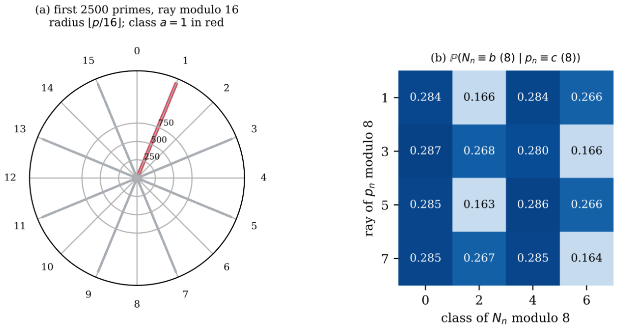
Ray portrait modulo 16 and the class of Nn. What is plotted: (a) the first 2500 primes at angle 2π(p mod 16)/16 and radius ⌊p/16⌋; the eight occupied spokes are the odd classes, and the class a = 1 of the restricted summand is drawn in red; (b) the conditional probability that Nn = pn + pn+1 lies in the class b modulo 8 given that pn lies in the ray c modulo 8, over all pairs of consecutive primes >7 with Nn ≤ 6 ⋅ 106. What it shows: only the φ(16) = 8 rays are occupied (Proposition 5.1), and the class b = 2 is reached with probability 0.166 from the rays 1,5 but 0.268 from the rays 3,7. Connection: Propositions 5.1 and 10.6.
Remark 5.5. [Honest Caveat] The slight excess of the rays 3 and 7 among the first 1000 primes (about 3 to 4 primes out of 250) is of the size of the fluctuations of the counting function and is not claimed to be systematic; at X = 108 the four counts differ from π(X)/4 by at most 0.013%.
6. A Transfer Principle and Almost-All Theorems
Lemma 6.1 (Anchoring). [Proved] For every n ≥ 2: (i) Nn is even; (ii) Nn+1 − Nn = pn+2 − pn > 0, so n ↦ Nn is strictly increasing and injective; (iii) Nn < 3pn. More generally, for fixed k ≥ 1 and Nn,k:=pn + pn+k: Nn,k is even for n ≥ 2, strictly increasing in n, and Nn,k < (1 + 2k)pn.
Proof. For n ≥ 2 both primes are odd, giving (i). For (ii), Nn+1 − Nn = pn+2 − pn > 0. For (iii), Bertrand’s postulate gives pn+1 < 2pn, so gn < pn and Nn = 2pn + gn < 3pn. Iterating, pn+k < 2kpn and hence Nn,k < (1 + 2k)pn; parity and monotonicity are as before.
Theorem 6.2 (Transfer principle). [Proved] Let q,a be as in the definition. Let 𝒜 be a set, s:𝒜 → [1,∞) a “size” function and f:𝒜 → 2ℕ a map such that, for some constants m ≥ 1, κ ≥ 1 and λ ≥ 0, #f−1(N) ≤ m for every N and f(n) ≤ κs(n) + λ for every n ∈ 𝒜. Then for all X ≥ 1 #{n ∈ 𝒜:s(n) ≤ X, Ra,q(f(n)) = 0} ≤ m⋅#a,q(κX + λ). (9) The inequality holds for every q ≥ 1 and every a with gcd(a,q) = 1, and the constants do not depend on any residue class of the elements of 𝒜.
Proof. Let F(X) be the set on the left. For n ∈ F(X), f(n) is even, satisfies f(n) ≤ κX + λ and Ra,q(f(n)) = 0, so f(n) ∈ a,q(κX + λ). Each element of a,q(κX + λ) has at most m preimages, whence #F(X) ≤ m #a,q(κX + λ).
Corollary 6.3 (Consecutive primes, uniform in the ray). [Proved] For every c and every X ≥ 3, #{pn ≤ X:pn≡c (q), Ra,q(Nn) = 0}≤#a,q(3X), and for k ≥ 1, #{pn ≤ X:pn≡c (q), Ra,q(pn + pn+k) = 0}≤#a,q((1 + 2k)X).
Proof. Take 𝒜 = {n ≥ 2}, s(n) = pn and f(n) = Nn (respectively Nn,k), which is injective by Lemma 6.1 and satisfies f(n) < 3s(n) (respectively <(1 + 2k)s(n)). Restricting to pn≡c (q) only shrinks the counted set, so (9) applies with m = 1, λ = 0 and κ = 3 (respectively 1 + 2k).
Corollary 6.4 (Shifted primes). [Proved] For every odd integer h (positive or negative) and X ≥ 1, #{p ≤ X:p > max(|h|,2), Ra,q(p + h) = 0}≤#a,q(X + |h|), uniformly over the rays of p modulo q.
Proof. For an odd prime p and odd h, p + h is even and p ↦ p + h is injective; apply Theorem 6.2 with 𝒜 the set of primes p > max(|h|,2), s(p) = p, f(p) = p + h, m = 1, κ = 1, λ = |h|.
Corollary 6.5 (Almost-all statements). [Proved] Let q = 2k and gcd(a,q) = 1. For every ray c with gcd(c,q) = 1 and every A > 0, #{pn ≤ X:pn≡c (q), Ra,q(Nn) = 0}≪q,AX(logX)−A = o(π(X;q,c)), so for almost all primes pn in every ray the even integer Nn = pn + pn+1 has a restricted Goldbach representation with first summand in the class a (q). The same holds for pn + pn+k with k fixed, and for p + h with h odd fixed.
Proof. By Corollary 6.3 and Corollary 4.12, the left side is at most #a,q(3X)≪q,A3X(log3X)−A≪X(logX)−A. Taking A = 2 and using π(X;q,c)∼X/(φ(q)logX) (Proposition 5.2) gives the o-statement. The statements for pn + pn+k and p + h are identical, using Corollary 6.3 and Corollary 6.4.
Remark 6.6 (Scope and triviality). [Honest Caveat] (i) By Proposition 2.3 the conclusion for Nn is automatic when pn or pn+1 lies in the class a; only the pairs of rays (c,c') with c≢a≢c' carry content. (ii) The transfer inequality holds for every modulus q, but for a modulus with an odd prime factor the exceptional set has positive density (Corollary 3.2), so Corollaries 4.12 and 6.5 are statements about q = 2k. (iii) None of this bears on the pointwise question whether Ra,q(Nn) > 0 for all large n; an infinite subsequence of exceptional n of density zero is not excluded.
Remark 6.7 (Gap bound of Baker–Harman–Pintz). [Proved] Since for large n [1], for every ε > 0 one has Nn < (2 + ε)pn for n ≥ n0(ε); the constant κ = 3 in Corollary 6.3 may then be replaced by 2 + ε for large X, with n0(ε) not asserted to be effective. Since log((2 + ε)X) = logX + O(1), this changes the conclusion of Corollary 6.5 only by a bounded factor, and the elementary constant 3 suffices
7. Computational Verification
Proposition 7.1 (Anchoring inequalities). [Comp. Verified, sieve; zero exceptions] Over all 216,814 pairs of consecutive primes with pn ≥ 3 and pn+1 ≤ 3 ⋅ 106, and over all 5,761,453 such pairs with pn+1 ≤ 108: Nn+1 − Nn > 0 (minimum increment 4), Nn/pn < 3 (maximum ratio 8/3, attained at the smallest admissible n), and Nn is even.
Proposition 7.2 (Brute-force check for q = 8, a = 1). [Comp. Verified; R computed by convolution in double precision; range n ≤ 5000] Table 3 lists, for the first K primes, the number of n ∈ [2,K − 1] for which Nn has no representation Nn = p1 + p2 with p1≡1 (8). The exceptional values are the same at every K: Nn ∈ {8,12,18,42,68}; no new exception occurs as K grows by a factor 100. None of the exceptions has pn≡1 or pn+1≡1 (8), in accordance with Proposition 2.3.
Proposition 7.3 (The full exceptional sets for q = 4,8,16,32). [Comp. Verified, even N ≤ 6 ⋅ 106, a = 1; Ra,q by double-precision FFT, every nonzero value at least log2log5 > 1.1] The sets 1,q(6 ⋅ 106) have 5, 25, 45, 115 elements for q = 4,8,16,32 and largest elements 62, 458, 1058, 3074; for (q,a) = (16,9) there are 53 elements, the largest being 1298. For q = 8 the elements are 4,6,8,10,12,14,16,18,26,32,38,42,50,56,62,66,68,74,98,122,188,218,242,362,458. No exceptional element occurs above the stated maximum up to 6 ⋅ 106 (Figure 2).
Proposition 7.4 (Shifted primes, q = 8, a = 1). [Comp. Verified, all primes 11 ≤ p ≤ 6 ⋅ 106 − 20 (412,844 primes); R1,8(N) by double-precision FFT for N ≤ 6 ⋅ 106; every nonzero value is at least log17log2 > 1.9, so values below 1 are exact zeros] For each shift h in Table 4, the number of primes p with R1,8(p + h) = 0 is small and the largest exceptional value of p + h is at most 458; no exception occurs above 458 in the range.
Remark 7.5. [Honest Caveat] Corollary 6.5 is asymptotic; its numerical onset depends on explicit constants in Theorem 4.10, which are ineffective, and need not lie in the tested range. The verification above tests only the finite ranges stated.
8. Moduli with an Odd Prime Factor along Nn
Theorem 8.1 (Obstruction along consecutive primes). [Proved] Let q have an odd prime factor 𝓁, gcd(a,q) = 1, and let n ≥ 2 with pn,pn+1 ≠ 𝓁. Write c≡pn and c'≡pn+1 modulo 𝓁. If c + c'≡a (𝓁), then every representation counted by Ra,q(Nn) has
, so that and in particular Ra,q(Nn) = Oq(logNn).
Proof. Suppose Nn = p1 + p2 with p1≡a (q). Then p1≡a (𝓁) and Nn≡c + c'≡a (𝓁), hence p2 = Nn − p1≡0 (𝓁). As p2 is prime, p2 = 𝓁 and p1 = Nn − 𝓁.
Corollary 8.2 (The obstructed set is infinite for 𝓁 = 3). [Proved] Let q = 3, a = 1. Then Nn≡1 (3) if and only if pn≡pn+1≡2 (3), and there are infinitely many such n. Consequently Ra,q(Nn) = O(logNn) for infinitely many n, and no asymptotic Ra,q(Nn)≍Nn/φ(q) can hold along Nn.
Proof. For pn,pn+1 > 3 the residues are 1 or 2 modulo 3, and c + c'≡1 (3) only for c = c' = 2. Infinitely many pairs of consecutive primes lie in the class 2 modulo 3 by Shiu’s theorem [13]. Apply Theorem 8.1.
Proposition 8.3 (Exact description for q = 3, a = 1). [Comp. Verified, all 216,813 pairs pn > 3, Nn ≤ 6 ⋅ 106; zero exceptions] Ra,q(Nn) = 0 holds if and only if Nn≡1 (3) and Nn − 3 is composite. In particular no n outside the class pn≡pn+1≡2 (3) has Ra,q(Nn) = 0, and the predicted characterisation has 0 mismatches (there are 36,809 zeros). Table 5 gives the fractions of obstructed indices and of exceptional indices in four ranges of Nn; over all even N ≤ 6 ⋅ 106 with N ≥ 103 the fraction with R1,3(N) = 0 is 0.2646, and one third of even integers satisfy N≡1 (3).
Figure 3.
Obstruction along consecutive primes for q = 3, a = 1. What is plotted: the fraction of n with Nn≡1 (3) and with R1,3(Nn) = 0, in logarithmic windows of Nn from 103 to 6 ⋅ 106, against the values 1/3 (generic even integers) and 1/4 (independent rays). What it shows: the obstructed fraction stays well below 1/3 and rises slowly towards 1/4. Connection: Proposition 8.3 and Remark 8.4.
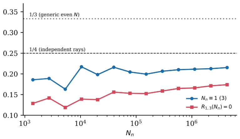
Remark 8.4. [Honest Caveat] Along Nn the obstructed fraction is the joint frequency of the diagonal pair of rays (2,2) modulo 3, which by the Lemke Oliver–Soundararajan bias is suppressed below 1/4 and, conditionally on the Hardy–Littlewood conjecture, tends to 1/4 slowly [8]; it is not the density 1/3 that the obstruction assigns to a generic even integer. The infinitude in Corollary 8.2 is proved; the density is not.
Proposition 8.5 (The case 𝓁 = 5). [Comp. Verified, all 216,812 pairs of consecutive primes pn > 5 with Nn ≤ 6 ⋅ 106] For q = 5 and a = 1,2,3,4, the fraction of n with Nn≡a (5) is 0.1735, 0.1885, 0.1865, 0.1733 and the fraction with Ra,5(Nn) = 0 is 0.1358, 0.1507, 0.1504, 0.1361. The prediction of Theorem 8.1, namely Ra,5(Nn) = 0 if and only if Nn≡a (5) and Nn − 5 is not prime, has exactly three failures in the range, all with Ra,5(Nn) = 0 although Nn≢a (5): Nn = 152 = 73 + 79 for a = 1, and Nn = 18 = 7 + 11 and Nn = 68 = 31 + 37 for a = 4. The fraction of obstructed indices is below the independent-rays value 1/4 for every a.
Remark 8.6. [Honest Caveat] Theorem 8.1 proves only that Nn≡a (𝓁) forces Ra,q(Nn) ∈ {0,(log(Nn − 𝓁))log𝓁}; the converse (non-obstructed Nn have Ra,q(Nn) > 0) is not proved, and the three exceptions above are small values at which it fails for 𝓁 = 5. For 𝓁 = 3 no failure was found in the tested range (Proposition 8.3)
Remark 8.7 (Comparison with [18]). [Comp. Verified, even N ≤ 2000, N≡1(3)] In [18, Remark 3.4] it is reported that for q = 3,a = 1 every nonempty representation list of such N is {(N − 3,3)}, and that R1,3(N) = 0 for 186 of the 333 even N ≤ 2000 with N≡1(3), a proportion 186/333≈0.559. Both statements were recomputed here by direct summation over the primes below 2000 and agree with [18]; they are the case 𝓁 = 3,a = 1 of Theorem 3.1.
9. Digit Repulsion, Gaps and Admissibility
9.1. The Transition Matrix
For n = 10 and a prime p > 5 write ray(p) = p mod 10 ∈ {1,3,7,9}.
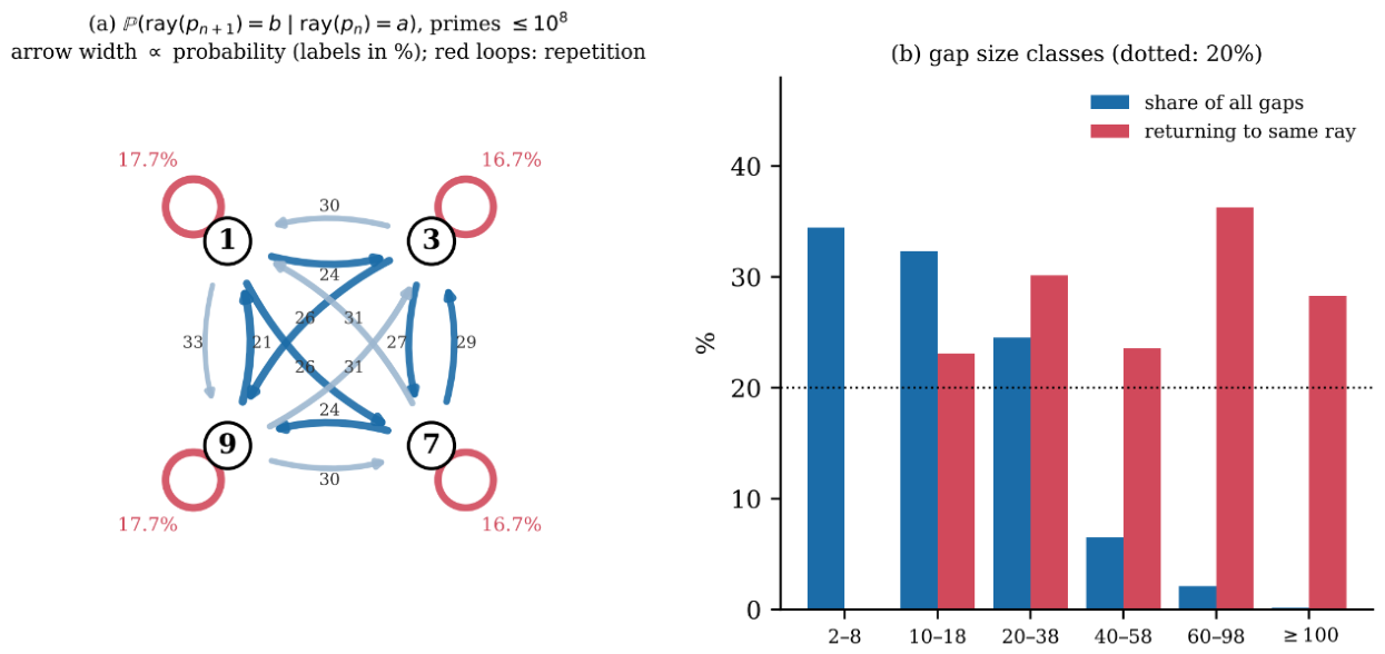
Proposition 9.1 (Digit repulsion). [Comp. Verified, all 5,761,451 pairs of consecutive primes >5 and ≤108] Table 6 gives the conditional transition matrix. The diagonal is suppressed to between 16.7% and 17.7% against 25% under independence, and every off-diagonal entry exceeds 20.8%; the qualitative bias reported in [8] is reproduced at 5.76 times the scale of the original data set.
Proposition 9.2 (Decay with lag). [Comp. Verified, same 5,761,451 primes] The probability that ray(pn+𝓁) = ray(pn) equals 17.18, 23.28, 24.50, 24.38, 24.40, 24.48, 24.58, 24.63 (%) for 𝓁 = 1,…,8.
Proposition 9.3 (Ray–gap identity). [Proved] For n with pn > 5: gn≡ρn+1 − ρn (mod 10), where ρn = ray(pn). In particular ρn+1 = ρn if and only if 10∣gn, and then gn ≥ 10; the ray of pn+1 is determined by ρn and gn mod 10, and conversely.
Proof. gn = pn+1 − pn reduces modulo 10 to ρn+1 − ρn. If ρn+1 = ρn then 10∣gn > 0.
Figure 4.
Digit repulsion as a flow on the four rays. What is plotted: (a) the four occupied rays modulo 10 as nodes, with an arrow from the ray a to the ray b of width proportional to ℙ(ray(pn+1) = b∣ray(pn) = a) (labels in %) and a red loop of width proportional to the probability of repeating the ray, for all consecutive primes 5 < pn < pn+1 ≤ 108; (b) for six classes of gap size, the share of all gaps (blue) and the proportion of those gaps that return to the same ray (red), against the independent value 20%. What it shows: the loops are the thinnest arrows (between 16.7% and 17.7%); the gaps 2,4,6,8 make up 34.4% of all gaps and cannot return. Connection: Propositions 9.1, 9.3 and 9.6.
9.2. Mean Gap by Ray of Origin
Proposition 9.4 (Gap by ray). [Comp. Verified, all pairs with pn > 5 and pn+1 ≤ 2 ⋅ 107 (1,270,603 pairs)] The global mean gap is 15.741. Conditioned on ray(pn) = 1,3,7,9 the mean gap is 15.474, 16.523, 14.836, 16.129, with deviations z = −11.5, +33.2, −38.4, +16.6 standard errors of the per-ray sample mean; the counts per ray are 317,587, 317,743, 317,690 and 317,583.
Remark 9.5 (Mechanical origin). [Comp. Verified] Table 7 conditions the mean gap on the pair (ray of pn, ray of pn+1). The diagonal entries (19.88 to 21.10) exceed every off-diagonal entry (12.86 to 18.90). The reason is elementary: a return to the same ray forces gn≡0 (10), and the smallest such gap is 10, whereas a change of ray admits gaps 2,4,6,8. Averaging the rows of Table 7 against the empirical transition frequencies of Table 6 reproduces the per-ray means of Proposition 9.4 (law of total expectation). The dependence of the mean gap on the ray of pn is therefore a corollary of the transition bias and the divisibility constraint, and is not an independent phenomenon.
Proposition 9.6 (Repetition of the ray by size of the gap). [Comp. Verified, all consecutive primes 5 < pn < pn+1 ≤ 108] By Proposition 9.3, ρn+1 = ρn if and only if 10∣gn. Table 8 gives, for six classes of gap size, the share of all gaps in the class and the proportion of those gaps that return to the same ray. The gaps 2,4,6,8 make up 34.4% of all gaps and none of them can return; overall 17.18% of the gaps are multiples of 10 (the value 17.18% of Proposition 9.2 at lag 1), against 20% if the five even residues of gn modulo 10 were equally likely. Among the gaps of size at least 20 the proportion returning to the same ray is between 23% and 37% in every class, above 20%.
Remark 9.7. [Honest Caveat] Proposition 9.6 displays the arithmetic part of the repulsion: more than a third of all gaps are too short to return to the ray. It does not prove that this accounts for the whole bias, nor does it replace the mechanism of Lemke Oliver and Soundararajan [8], which concerns the correlations of the gap sizes.
9.3. Cumulative Admissibility
For a prime q0 > 2 let
be the Hardy–Littlewood admissibility function of h with the local factor at q0 removed.
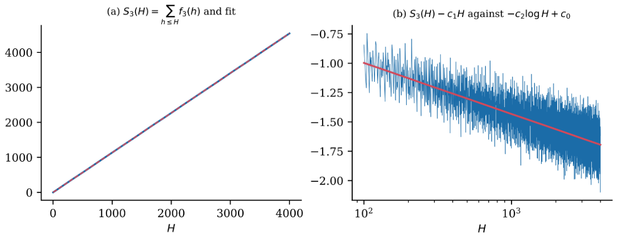
Proposition 9.8 (Cumulative sum). [Comp. Verified, least squares over every integer 100 ≤ H ≤ 4000] Fitting gives c1 = 1.136085, c2 = 0.188854, c0 = −0.127389 with R2 = 0.99999999 for q0 = 3, and c1 = 1.420105, c2 = 0.282050, c0 = −0.298717 with R2 = 0.99999996 for q0 = 5; in both cases c2 > 0, i.e. the secondary term has the sign opposite to that extrapolated from the main term.
Proposition 9.9 (Dirichlet series of and closed forms of the constants). [Proved] For ℜs > 1, where converges absolutely, is holomorphic in ℜs > −1/2 and positive for real s > −1/2. Hence D extends meromorphically to ℜs > −1/2 with exactly two poles, both simple, at s = 1 and at s = 0. [Comp. Verified] With and , evaluated with the products taken over all primes ≤108, one finds , for q0 = 3 and , for q0 = 5.
Proof. The function depends only on the set of odd primes ≠q0 dividing h, so D(s) is an Euler product whose local factor is at p = 2, at p = q0 and, at an odd prime p ≠ q0,
because . Collecting the factors gives ζ(s) times the stated product. Writing x = p−s, , so the product defining converges absolutely for ℜs > −1/2, since and converge for σ > −1/2. Each factor is positive for real s > −1, and the product equals after restoring the factors 1 − 2−1−s and and the factors of ζ(s + 1).
Remark 9.10. [Honest Caveat] Proposition 9.9 identifies the poles of D at s = 1 and s = 0 and shows that the residue of D(s)Hs/s at the double pole s = 0 contributes , with the sign of ζ(0) = −1/2 opposite to that of the main term . It does not prove the asymptotic formula for the sharp cutoff h ≤ H: that requires control of the contour integral, which [8,14] obtain for a smooth weight. Numerically agrees with the fitted c1 in all printed digits and is within 0.3% (q0 = 3) and 0.7% (q0 = 5) of the fitted c2 of Proposition 9.8, a difference compatible with the O(1) remainder.
Figure 5.
Cumulative admissibility sum for q0 = 3. What is plotted: (a) computed directly for H ≤ 4000 and the least-squares fit c1H − c2logH + c0 over 100 ≤ H ≤ 4000; (b) the same data after subtracting c1H, on a logarithmic H-axis, against −c2logH + c0. What it shows: the curves in (a) are indistinguishable at this scale, and (b) isolates the secondary term, with c2 > 0. Connection: Propositions 9.8 and 9.9.
Remark 9.11 (Role in the bias). [Honest Caveat] Proposition 9.8 is a numerical fit. The mechanism of Lemke Oliver and Soundararajan [8] derives the transition probabilities from such secondary terms under the Hardy–Littlewood prime tuples conjecture, so the transition formulas are conditional and are not asserted here as theorems. For q0 = 3 the two-ray transition matrix (joint probabilities, diagonal/off-diagonal) was recomputed at four scales (Table 9) and moves monotonically towards 25% in every cell as N grows.
Proposition 9.12 (Comparison with the Lemke Oliver–Soundararajan prediction, q0 = 3). [Comp. Verified, primes 3 < pn < pn+1 ≤ N for N = 3 ⋅ 106,107,108,109; the scale 109 uses a segmented sieve] Let d(N) = 1/8loglogN/logN and let the prediction be the joint frequency 1/4 − d(N) for the cells (1,1) and (2,2) and 1/4 + d(N) for the cells (1,2) and (2,1). Table 10 gives the mean absolute error of the four observed joint frequencies against this prediction and against the value 1/4. The error against the prediction is smaller than the error against 1/4 at every N, by the factors 0.397, 0.381, 0.353, 0.334, and both errors decrease with N.
Figure 6.
Mod-3 joint frequencies of consecutive primes at four scales. What is plotted: (a) the observed joint frequencies of (pn mod 3,pn+1 mod 3) for the cells (1,1), (2,2) and (1,2) = (2,1) at N = 3 ⋅ 106,107,108,109, with the prediction 1/4∓d(N) (dotted); (b) the mean absolute error against the prediction and against 25%. What it shows: the diagonal cells are suppressed, the off-diagonal cells inflated, all moving towards 25%; the prediction reduces the error by a factor 0.33 to 0.40. Connection: Proposition 9.12 and Remark 9.13.
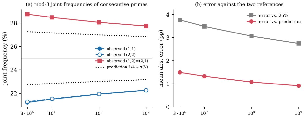
Remark 9.13. [Honest Caveat] The prediction is the leading secondary term of the argument of Lemke Oliver and Soundararajan as presented by Tao [14], and it is derived under the Hardy–Littlewood prime tuples conjecture; it is not a theorem. The agreement in Proposition 9.12 is with the leading term only, and a residual of about 1 percentage point remains at N = 108, which the formula does not describe.
10. The Second Moment Modulo q
Let q = 2k, Da,q(N):=(Ra,q(N) − Ma,q(N))/Ma,q(N) and write b≡N (mod q).
10.1. A Symmetry
Proposition 10.1 (Symmetry of the restricted sum). [Proved] For classes a,a' modulo q let . Then Ra,a'(N) = Ra',a(N). In particular, for N≡2a (q) the representations counted by Ra,q(N) are closed under (p1,p2) ↦ (p2,p1), and , whereas for N≢2a (q) each unordered pair {p,p'} with p≡a, p'≡N − a≢a is counted exactly once.
Proof. Exchange p1,p2 in the defining sum. If N≡2a then p1≡a implies p2 = N − p1≡a, so both orders are counted; the term p1 = p2 = N/2 is counted once. If N≢2a, the class of p2 differs from that of p1, and only one order of an unordered pair is counted.
Remark 10.2 (Heuristic consequence). [Honest Caveat] If the unordered pair counts fluctuated like independent Poisson variables with the same mean μ, the doubling in Proposition 10.1 would multiply the variance of Ra,q(N) by 4 ⋅ (μ/2)/μ = 2 when N≡2a (q). This is a heuristic explanation of the numerical ratio below, not a proof.
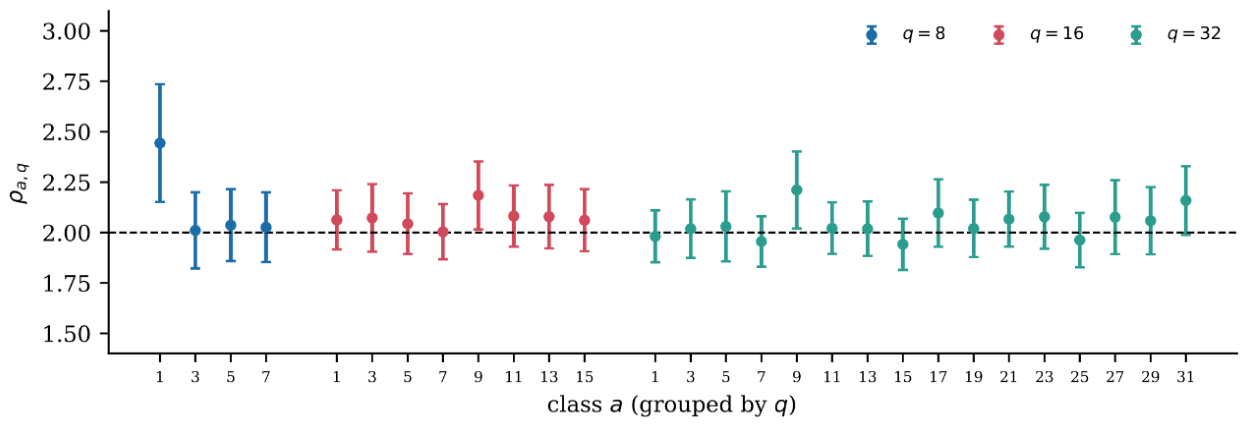
Proposition 10.3 (Second moment by class of N). [Comp. Verified; Ra,q(N) computed by FFT convolution of the weighted prime indicators for all even N ≤ 6 ⋅ 106, Ma,q from an exact factorisation sieve] (i) For q = 8, a = 1 and even N ∈ [105,6 ⋅ 106], the mean of (in units of 10−5) is 9.70, 24.21, 9.76, 9.29 for N≡0,2,4,6 (8), and the mean of D1,8 (in units of 10−3) is −2.991, −5.715, −2.920, −2.999. (ii) For even N ∈ [106,6 ⋅ 106], let ρa,q be the mean of on N≡2a (q) divided by its mean on the other classes. For q = 8, a = 1,3,5,7: ρ = 2.44, 2.01, 2.04, 2.03; for q = 16 and all eight a: 2.06, 2.07, 2.04, 2.00, 2.18, 2.08, 2.08, 2.06 (mean 2.07); for q = 32 and all sixteen a the mean is 2.04 and the range 1.94 to 2.21. Delete-one jackknife standard errors over 20 interleaved blocks are 0.17 to 0.29 for q = 8 and 0.12 to 0.19 for the values of a tested at q = 16,32; every value is within 1.6 standard errors of 2, including ρ1,8 = 2.44 ± 0.29.
Figure 7.
Variance ratio on the class N≡2a (q) for every admissible class. What is plotted: the ratio ρa,q of the mean of on N≡2a (q) to its mean on the other classes, for N ∈ [106,6 ⋅ 106] and for every odd a modulo q = 8 (blue), 16 (red), 32 (green), with delete-one jackknife error bars over 20 interleaved blocks, against the symmetry value 2 (dashed). What it shows: every one of the 28 values lies within 1.6 standard errors of 2. Connection: Proposition 10.3 and Remark 10.2.
Proposition 10.4 (Size of the second moment). [Comp. Verified; q = 8, a = 1, all even N ≤ X, X ≤ 6 ⋅ 106] Table 11 gives relative to X3 and to X3/logX. The second ratio decreases monotonically in X, from 4.68 × 10⁻⁴ at X = 2 × 10⁵ to 3.19 × 10⁻⁵ at X = 6 × 10⁶.
Figure 8.
Size and class dependence of the second moment, q = 8, a = 1. What is plotted: (a) for 2 ⋅ 105 ≤ X ≤ 6 ⋅ 106 on logarithmic axes with the line ∝X−1; (b) the mean of in units of 10−5 on the four classes of N modulo 8 (N ∈ [105,6 ⋅ 106]), the class N≡2a in red; (c) the variance ratio ρ1,q for q = 8,16,32 against the value 2. What it shows: the local exponent in (a) is about −0.85; the class N≡2 carries more than twice the variance of the others. Connection: Propositions 10.4 and 10.3.
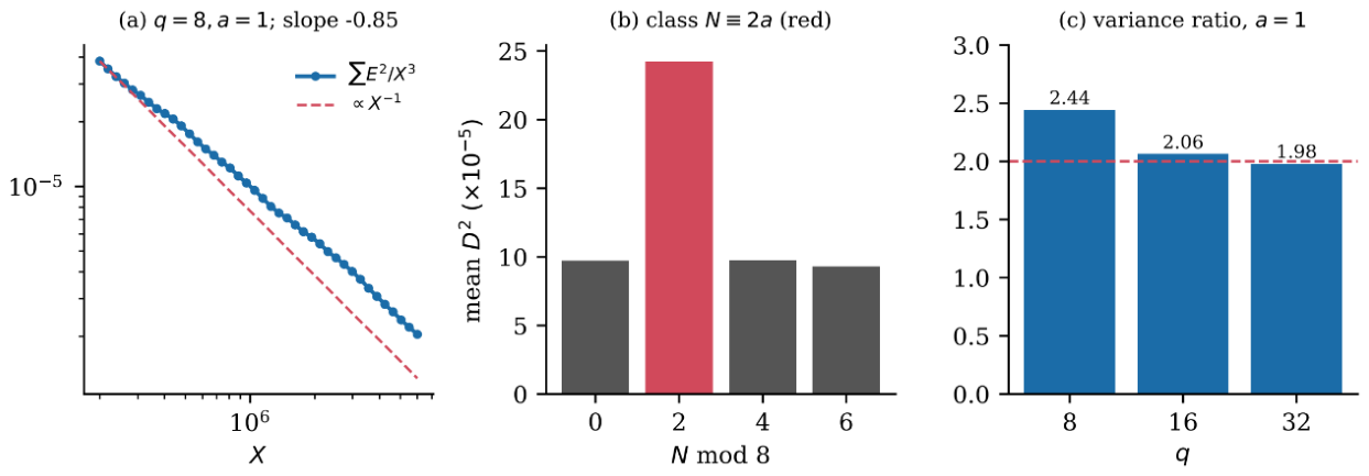
Remark 10.5. [Honest Caveat] Proposition 10.4 is a finite-range measurement and proves nothing about the limit. By Theorem 4.10, for every fixed A > 0 one has for q = 2k (the case q = 1 being classical, Remark 4.11); this is compatible with the decrease seen in Table 11, and it excludes any lower bound of order X3/logX for the second moment. The finite range does not by itself decide the true order between X3(logX)−A and a power saving in X; the measured local exponent −0.85 in X3 ⋅ X−0.85 is a statement about X ≤ 6 ⋅ 106 only.
10.2. From the Ray of pn to the Class of Nn
Since Nn≡c + c' (q) with c,c' the rays of pn,pn+1, the distribution of Nn mod q given c is read off the transition matrix of consecutive primes modulo q.
Proposition 10.6 (Class of Nn given the ray, q = 8). [Comp. Verified, all 216,811 pairs of consecutive primes >7 with Nn ≤ 6 ⋅ 106] Table 12 gives ℙ(Nn≡b (8)∣pn≡c (8)). For rays c = 1,5 the class b = 2 has probability 0.166 and 0.163, and for rays c = 3,7 it has probability 0.268 and 0.267: the classes b≡2 (8) arise from the pairs (1,1), (5,5), (3,7), (7,3), and the two diagonal pairs are suppressed by the digit-repulsion bias.
Proposition 10.7 (Second moment along Nn by ray, q = 8, a = 1). [Comp. Verified; 211,683 pairs of consecutive primes >7 with 105 ≤ Nn ≤ 6 ⋅ 106; jackknife over 20 interleaved blocks n mod 20] Put D = D1,8(Nn) and let be the mean of D2 over pn≡c (8), in units of 10−5. Then for c = 1,3,5,7, and the mean over all n is 10.79. The pairwise differences are: rays 1 − 3: −1.39 ± 0.18 (z = −7.8); 1 − 7: −1.70 ± 0.25 (z = −6.9); 5 − 3: −1.49 ± 0.19 (z = −8.0); 5 − 7: −1.80 ± 0.19 (z = −9.3); 1 − 5: +0.10 ± 0.16; 3 − 7: −0.31 ± 0.24. The second moment along Nn therefore depends on the ray of pn: rays 3 and 7 exceed rays 1 and 5.
Proposition 10.8 (Prediction by the class of Nn). [Comp. Verified; same sample] Let be the mean of over all even N ∈ [105,6 ⋅ 106] in the same cell, where a cell is a logarithmic window of N (15 windows with equally spaced logarithms) together with the class of N modulo 8 (respectively modulo 8,3 and 5). Then, in units of 10−5: (i) windows alone predict the overall mean as 14.22; (ii) adding the class modulo 8 gives 13.66, and predicts the ray differences 1 − 3, 1 − 7, 5 − 3, 5 − 7, 1 − 5, 3 − 7 as −1.68, −1.66, −1.75, −1.73, +0.07, +0.02; (iii) adding the classes modulo 3 and 5 gives 11.05 for the overall mean (observed 10.79), the per-ray means 10.36, 11.72, 10.34, 11.78 (observed 10.04, 11.43, 9.94, 11.74), and the ray differences −1.36, −1.41, −1.38, −1.43, +0.02, −0.05, against the observed values of Proposition 10.7. The differences observed minus predicted in (iii) for rays 1,3,5,7 are −0.32 ± 0.12, −0.29 ± 0.14, −0.41 ± 0.07 and −0.04 ± 0.15.
Remark 10.9 (Interpretation). [Honest Caveat] The ray of pn acts on the second moment through the class of Nn: the transition matrix of Proposition 10.6 sends more mass to Nn≡2 (8) from rays 3,7, and that class has twice the variance (Proposition 10.3). The ordering and size of the differences are predicted by the class modulo 8 alone to about 20% (−1.7 against observed −1.4 to −1.8). The inclusion of the classes modulo 3 and 5 was decided after seeing that windows and the class modulo 8 over-predict the level; at q = 8 it is therefore a fit choice and not a pre-specified prediction; Proposition 10.10 applies the same recipe, unchanged, at q = 16. The remaining discrepancy (−0.3 × 10⁻⁵ for rays 1,3,5, two to four standard errors) is about 3% of the level and is not explained. The sample is restricted to Nn ≥ 105 and is compared with a reference population in the same range of N, because D2 is larger by an order of magnitude at small N.
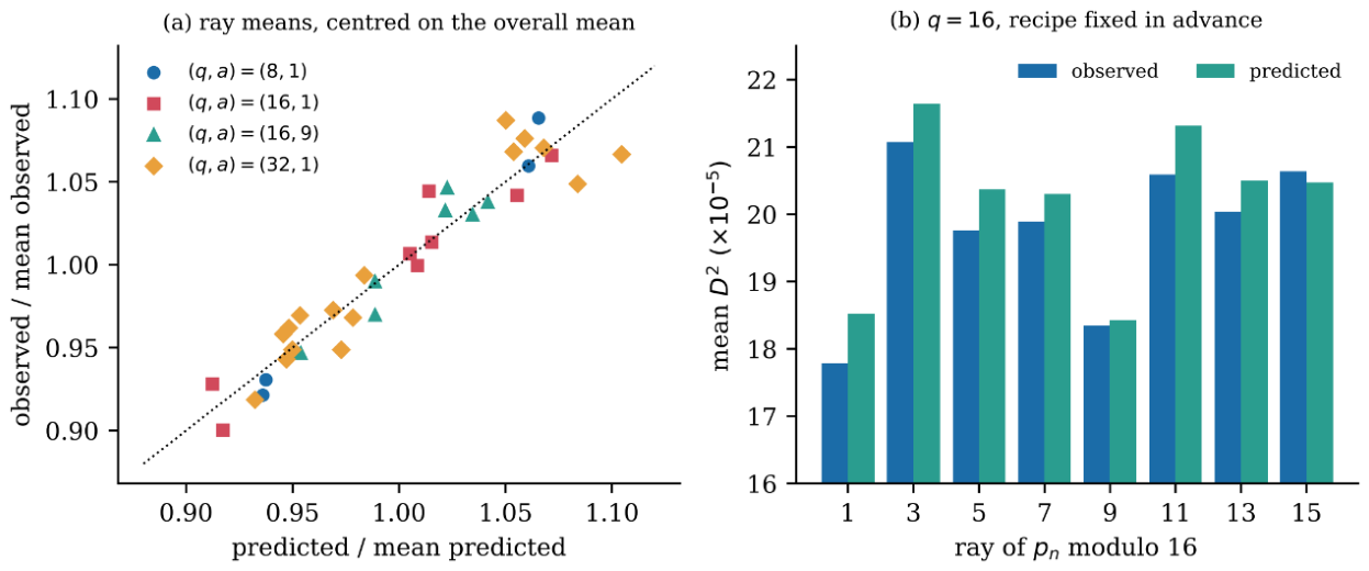
Proposition 10.10 (Prediction fixed in advance, q = 16, a = 1). [Comp. Verified; 211,683 pairs of consecutive primes >7 with 105 ≤ Nn ≤ 6 ⋅ 106; jackknife over 20 interleaved blocks] The recipe of Proposition 10.8(iii) was applied unchanged with the class modulo 8 replaced by the class of N modulo 16: cells are 15 logarithmic windows of N together with the classes of N modulo 16, 3 and 5, and the prediction for Nn is the mean of over all even N ∈ [105,6 ⋅ 106] in the same cell. Then, in units of 10−5: the overall mean is observed 19.77 and predicted 20.19; the means over the eight rays c = 1,3,5,7,9,11,13,15 of pn modulo 16 are observed 17.79, 21.07, 19.75, 19.90, 18.34, 20.59, 20.03, 20.64 and predicted 18.52, 21.64, 20.37, 20.29, 18.42, 21.31, 20.50, 20.48. The spread between the largest and smallest ray mean is 3.28 observed and 3.22 predicted, and the correlation between observed and predicted ray means is 0.962. The differences of the ray means against ray 1 (rays 3,5,7,9,11,13,15) are observed +3.28, +1.96, +2.10, +0.55, +2.80, +2.24, +2.85 (z = +6.1, +4.6, +3.6, +1.0, +4.6, +3.5, +4.2) and predicted +3.12, +1.84, +1.77, −0.10, +2.79, +1.98, +1.95. The differences observed minus predicted for the eight ray means range from −0.73 to +0.16, with standard errors 0.20 to 0.39; the largest in absolute z is ray 5 (−0.61 ± 0.20, z = −3.1).
Proposition 10.11 (The same recipe at other pairs (q,a)). [Comp. Verified; same sample of 211,683 pairs and same reference population; recipe of Proposition 10.10 unchanged, with the class modulo q in place of the class modulo 16] Table 13 lists, for four pairs (q,a), the overall means of along Nn (observed and predicted, in units of 10−5), the relative difference observed minus predicted with its delete-one jackknife z-value, the spread between the largest and smallest ray mean (observed and predicted), and the correlation between observed and predicted ray means over the reduced rays modulo q. In every case the observed overall mean is below the predicted one, by 2.1% to 3.0%, and the number of rays whose observed mean is below the prediction is 4/4, 7/8, 8/8 and 15/16 respectively.
Figure 9.
Observed against predicted second moment along Nn, by ray of pn. What is plotted: (a) for (q,a) = (8,1),(16,1),(16,9),(32,1) the ray means observed and predicted, each divided by its own overall mean (points on the dotted diagonal are perfectly predicted); (b) for q = 16, a = 1, the observed and predicted mean of (units of 10−5) on the eight rays of pn, the recipe being fixed in advance. What it shows: the recipe reproduces the pattern among rays at every pair, with a small systematic over-prediction of the level. Connection: Propositions 10.8, 10.10, 10.11 and Remark 10.13.
Proposition 10.12 (Effect of further small primes, exploratory). [Comp. Verified; exploratory, the additional moduli were chosen after seeing Table 13] Adding the class of N modulo 7, and then modulo 7 and 11, to the cells of the prediction changes the relative difference observed minus predicted (with z in parentheses) from −2.4% (−4.0) to −1.6% (−2.8) and −1.3% (−2.3) at (q,a) = (8,1); from −2.1% (−3.5) to −1.0% (−1.7) and −0.6% (−1.6) at (16,1); and from −3.0% (−5.1) to −2.0% (−3.6) and −1.4% (−2.9) at (16,9).
Remark 10.13. [Honest Caveat] The prediction at q = 16 uses the recipe of q = 8 without adjustment, so it is a test and not a fit. It reproduces the ordering, the spread and the level of the second moment by ray, but it over-predicts by about 3% for most rays, and the eight differences are not independent (they share a common shift), so the z-values above must not be combined as independent evidence. The over-prediction recurs at every pair tested (Table 13) and decreases monotonically when the classes modulo 7 and 11 are added (Proposition 10.12), which is consistent with Nn = 2pn + gn differing from a generic even integer through its residues modulo small primes; this reading is exploratory, and a residual of about 1% to 1.4% remains at the pairs tested. At q = 8 the spread among rays is under-predicted (1.43 against 1.80), while at q = 32 it is over-predicted (6.81 against 6.50). All results are for one range of N, 105 ≤ N ≤ 6 ⋅ 106.
11. Predicting the Next Ray and the Gap
Let ray(p) = p mod 10 for p > 5, and write ρn = ray(pn) ∈ {1,3,7,9}.
Proposition 11.1 (Prediction out of sample). [Comp. Verified; recipe fixed before the run; all pairs (pn,pn+1) with 5 < pn < pn+1 ≤ 108 (5,761,451 pairs); temporal split: training pn ≤ 5 ⋅ 107 (3,001,131 pairs), test pn > 5 ⋅ 107 (2,760,320 pairs)] For the context (ρn,ρn−1,…,ρn−k+1) the predictor of ρn+1 is the most frequent next ray in the training set, and the predictor of gn/logpn is the training mean in the same context. Table 14 gives, on the test set, the accuracy for ρn+1 (baseline 0.2500, standard error 0.0003), the information gain in bits over the marginal distribution of ρn+1 (uniform: 2 bits), and the coefficient of determination R2 for gn/logpn against the training global mean. Accuracy is 0.311 with one ray and 0.316 with four, an excess of about 6.5 points over 0.25; the information gain is 0.036 bits out of 2; and R2 for the normalised gap is at most 0.0019. The most likely next ray given ρn = 1,3,7,9 is 7,9,9,1, with test accuracy 0.3075, 0.3072, 0.3020, 0.3277.
Proposition 11.2 (Reference level for the gap). [Comp. Verified; same split] Using the exact value of gn mod 10 (which is not available before pn+1 is known) as the context, the training means of gn/logpn by class give R2 = 0.0355 on the test set.
Remark 11.3 (Interpretation). [Honest Caveat] The rays of the past predict the ray of the next prime better than chance, and essentially all of this comes from the last ray: the gain from k = 1 to k = 4 is 0.003 bits, in line with the decay with lag in Proposition 9.2. The size of the gap is not predicted: the class of gn mod 10, even if known, would explain 3.6% of the variance of gn/logpn, and the rays of the past explain at most 0.19%, which is about a twentieth of that reference. The decrease at k = 6 reflects the 4,096 contexts estimated from the training set. The accuracy of about 31.6% is a measurement of the Lemke Oliver–Soundararajan bias as a predictor and is not a new mechanism; it is not asserted to persist at larger scales, where the bias decays. The context of one ray is fixed by the transition matrix of Table 6, whose row maxima (31.0%, 31.0%, 30.4%, 33.1% in sample) are reproduced out of sample.
12. The Main Term Along Shifted Primes
By Corollary 6.4 the integers p + h (h odd fixed) are covered by the almost-all theorem, but the shifted primes have density zero and Corollary 4.12 is silent on how the size of the main term behaves along them. Since for q = 2k, the whole dependence on the shift sits in the amplitude 𝔖(p + h), which we now study. Throughout, h ≥ 1 is odd and as in (2).
Let be independent Bernoulli variables with ℙ(B𝓁 = 1) = 1/(𝓁 − 1), and define
The choice ℙ(B𝓁 = 1) = 1/(𝓁 − 1) is the density of primes p with 𝓁∣p + h, and the primes 𝓁∣h are omitted because 𝓁∣p + h forces p = 𝓁.
Proposition 12.2 (The model). [Proved] (i) Yh is a.s. finite and Yh > 1 a.s. (ii) For every complex z the product converges, and Mh is entire of order at most 1. (iii) .
Proof. (i) by (5), so logYh < ∞ a.s. Also since . (ii) Theorem 12.8(a) below gives for every real s, hence ; dominated convergence applied to the partial products (dominated by ) and independence give the product formula and analyticity. The bound |Mh(z)| ≤ Mh(ℜz) ≤ exp(|z|log|z| + O(|z|)) of Theorem 12.8(a) shows order at most 1. (iii) is immediate.
Theorem 12.3 (Limit law). [Proved] Let h ≥ 1 be odd. As x → ∞, the random variable 𝔖(p + h), with p uniform among the primes ≤x, converges in distribution to Yh.
Proof. Fix y ≥ 3 and put , .
Step 1 (bounded range). For p > h no prime 𝓁∣h divides p + h. The indicators are determined by p modulo , and 𝓁∣p + h is one of the 𝓁 − 1 unit classes modulo 𝓁. By the prime number theorem in arithmetic progressions the primes are asymptotically equidistributed among the φ(my) unit classes modulo my, so by the Chinese remainder theorem the vector of indicators converges in distribution to independent Bernoulli variables with parameters 1/(𝓁 − 1). Hence 𝔖y(p + h) ⇒ Yh,y.
Step 2 (tail). Take y ≥ 5. Let , since for 𝓁 ≥ 4. Put x' = x + h. For n = p + h ≤ x' there is at most one prime divisor , contributing at most . For with 𝓁∤h, Lemma 12.1 gives #{p ≤ x:𝓁∣p + h} ≤ 2x/(φ(𝓁)log(x/𝓁)) ≤ 4x/(φ(𝓁)logx). Hence as x → ∞. By Markov’s inequality, limsupxℙx(Dy > ε) ≤ 9/(εy) → 0 as y → ∞.
Step 3. Yh,y ↑ Yh almost surely as y → ∞, and hence in distribution. The approximation theorem for weak convergence [2], applied to log𝔖y(p + h), log𝔖(p + h) and logYh,y, followed by the continuous map exp, gives the theorem.
Lemma 12.4 (Uniform integrability). [Proved] Let h ≥ 1 be odd and λ > 0. Then . Consequently, for every m > 0, .
Proof. Only p > h matter. Choose y ≥ 2λ and put x' = x + h. Split the primes 𝓁∣n = p + h into 𝓁 ≤ y, , and . The first range contributes a factor at most , the last at most . For the middle range, write . Then , , the sum running over squarefree d with all prime factors in ; we used et − 1 ≤ 2t for . Terms with contribute at most τ(n)(2λ)ω(n)x'−1/2≪x'−1/2+ε. For , Lemma 12.1 gives ℙx(d∣p + h) ≤ 5/φ(d) for large x. Therefore for y = y(λ) large. The last statement follows from , by (5).
Theorem 12.5 (Convergence of all moments). [Proved] For odd h ≥ 1 and every m > 0, Proof. By Theorem 12.3, . By Lemma 12.4 applied with m replaced by m + 1, the family {𝔖(p + h)m} is uniformly integrable, so the expectations converge [2] to . The product formula is Proposition 12.2(ii).
Proposition 12.6 (Certified enclosures of Am(h)). [Comp. Verified] Let Q ≥ 2m + 3 and Am(h;Q) be the product at z = m truncated to 𝓁 ≤ Q. Then Am(h;Q) ≤ Am(h) ≤ Am(h;Q)exp(2m/(Q − 1)). With Q = 107 (double precision, fsum over the 664,578 odd primes ≤Q), Table 15 gives enclosures of Am(1) and Am(3).
Proof. For 𝓁 > Q we have (as ), so , and . The tabulated values are the truncated products and their inflation by this factor.
Proposition 12.7 (Dependence on the shift and amplification). [Proved; numerical value Comp. Verified] (i) If h,h' are odd and have the same set of odd prime divisors, then Yh and Yh' have the same law, and ; in particular A1(3) = A1(1)/3/2. (ii) Let with independent ℙ(C𝓁 = 1) = 1/𝓁 (the model for 𝔖(n) over all even n). Then 𝔼U = 1/C2 and 𝔼Um < Am(1) for every m > 0; in particular C2A1(1) ∈ [1.15048,1.15049] ⊂ (1,∞).
Proof. (i) is immediate from the product formula. (ii) . Termwise, . The numerical range follows from Propositions 2.2 and 12.6.
Theorem 12.8 (Moment generating function and tails). [Proved] There is an absolute constant C0 such that:
- for all odd h and real s ≥ 3, logMh(s) ≤ sloglogs + C0s; in particular for every real s;
- with, ℙ(Yh > y) ≤ exp(−exp(c0y)) for all y with exp(c0y) ≥ 3;
- for h = 1 and y ≥ 1, ℙ(Y1 > y) ≥ exp(−2exp(ey)). Hence for large y.
Proof. (a) For real s > 0, is a product of independent nonnegative factors, so by monotone convergence equals the product in [1,∞]; each factor is ≥1, whence Mh(s) ≤ M1(s). For 3 ≤ 𝓁 ≤ s + 2, and log(1 + et) ≤ t + log2 give a contribution ; summing over these 𝓁 and using Mertens’ theorem, this is ≤sloglogs + C1s. For 𝓁 > s + 2, t = s/(𝓁 − 2) < 1, , so the contribution of these primes is at most . This proves (a) with an absolute C0.
(b) By Markov’s inequality, ℙ(Yh > y) ≤ Mh(s)e−slogy ≤ exp(s(loglogs + C0 − logy)). Choose s = exp(c0y), so that loglogs = logy − C0 − 1; the exponent is −s.
(c) If B𝓁 = 1 for all 3 ≤ 𝓁 ≤ r then, by (5) and Mertens’ theorem, . Taking r=⌈exp(ey)⌉ this exceeds logy. The probability of this event is by Rosser–Schoenfeld [12], which is ≥exp(−2exp(ey)). The two-sided statement follows from (b) and (c).
Theorem 12.9 (Continuity). [Proved] Let Q(X;λ) = suptℙ(t ≤ X ≤ t + λ). There is an absolute constant 𝒜 such that for every odd h and , . In particular logYh, and hence Yh, has no atoms.
Proof. By independence, Q(S + T;λ) ≤ Q(S;λ) for a partial sum S and independent remainder T. Apply the Kolmogorov–Rogozin inequality [10], for 0 < λi ≤ λ, with λi = λ to the variables X𝓁 = B𝓁loga𝓁, 𝓁∤h. For λ < loga𝓁 the variable X𝓁 takes two values with probabilities and , so (recall 𝓁 ≥ 3). By (5), every prime 𝓁 < 1/λ satisfies loga𝓁 > λ, and by Mertens.
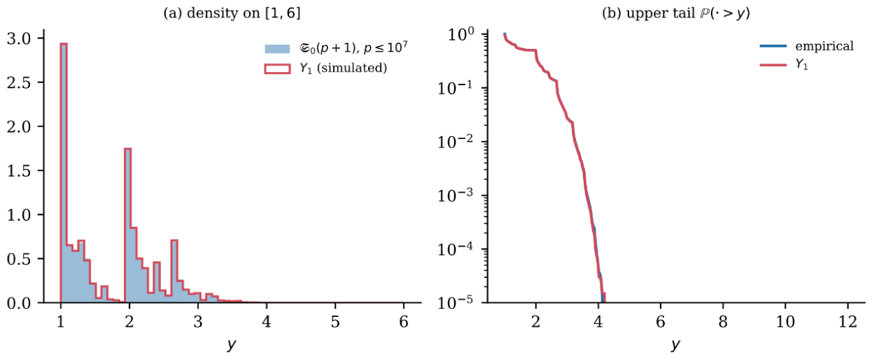
Corollary 12.10 (Law of the main term along p + h). [Proved] Let q = 2k (k ≥ 1), a odd, h ≥ 1 odd. For N = p + h, , so, as p → ∞, this ratio converges in distribution to Yh, its moments converge to Am(h), and for every y the limiting probability that the ratio exceeds y equals ℙ(Yh > y) ≤ exp(−exp(c0y)) (the law of Yh has no atoms by Theorem 12.9, so every y is a continuity point).
Proof. The identity is (2); the rest is Theorems 12.3, 12.5 and 12.8.
Remark 12.11. [Honest Caveat] The shifted primes have density zero, so Corollary 4.12 is silent on N = p + h. Corollary 12.10 says instead that the expected number of restricted representations of p + 1, normalised by its size, is on average C2A1(1)≈1.1505 times the value for a generic even integer (Proposition 12.7), and that its fluctuations are governed by the explicit law Y1, which is continuous and has a doubly exponentially thin upper tail. This is a statement about the main term; no claim is made about Ra,q(p + h) itself beyond Corollary 6.4.
Proposition 12.12 (Comparison with the primes up to 107). [Comp. Verified] Over the 664,578 odd primes p ≤ 107, the empirical moments of 𝔖(p + h) are 1.742811, 3.460872, 7.62999, 18.1785 for m = 1,2,3,4 at h = 1, and 1.161863, 1.384401, 1.69582, 2.1394 at h = 3, each inside the enclosures of Table 15 up to the finite-x effect. For h = 1, the Kolmogorov distance between the empirical distribution function and that of Y1 (estimated from 2 × 10⁵ independent samples of Y1 with all primes 𝓁 ≤ 2 × 10⁶, seed 12345), restricted to the interval [1.001,6], is 0.0100, against a Monte Carlo fluctuation of about 0.003. The interval starts at 1.001 because the truncated model places mass 0.1055 below 1.001 against 0.0980 empirically; the discrepancy reflects the slow convergence of the atom-like mass near 1 (integers with all odd prime factors large) and is consistent with a finite-x effect.
Figure 10.
The amplitude 𝔖(p + 1) and its limit law Y1. What is plotted: (a) the empirical density of 𝔖(p + 1) over the odd primes p ≤ 107 (filled) and of 2 × 10⁵ simulated samples of Y1 (outline) on [1,6]; (b) the upper tails ℙ(⋅>y) on a logarithmic scale. What it shows: the two laws agree to about 0.01 in Kolmogorov distance, and the tail falls faster than any exponential. Connection: Theorems 12.3 and 12.8 and Proposition 12.12.
13. Open Questions
Open Question 13.1 (Power saving for q = 2k). [Open] Prove for some Δq > 0, q = 2k, k ≥ 1 and every a, with full details for the character sums modulo q; the case q = 1 is the theorem of Montgomery and Vaughan [9], and the difficulty is to adapt the zero-density input to the character sums arising from Lemma 4.3. A power saving would give, via Corollary 6.3, .
Open Question 13.2 (Effective version). [Open] Theorem 4.10 is ineffective because it uses the Siegel–Walfisz theorem. Give an explicit X1 = X1(q,a,c) beyond which #a,q(3X) < π(X;q,c), i.e. not merely asymptotically; this requires an effective replacement of the Siegel–Walfisz input on the major arcs.
Open Question 13.3 (From almost all to all). [Open] Determine whether a,q is finite for q = 2k. Neither Theorem 4.10 nor Corollary 4.12 settles this: each bounds the count of exceptional N up to X and none rules out an infinite, arbitrarily sparse sequence of exceptions. A uniform pointwise lower bound Ra,q(N) > 0 for all sufficiently large even N would be at least as strong as the corresponding statement for the classical binary Goldbach problem. The data of Proposition 7.3 (the largest exceptional integers 62,458,1058,3074 for q = 4,8,16,32 in N ≤ 6 ⋅ 106) are compatible with finiteness and do not prove it.
Open Question 13.4 (Density of the obstruction). [Open] For q = 3, a = 1 decide whether the natural density of {n:pn≡pn+1≡2 (3)} exists; conditionally on the Hardy–Littlewood conjecture it is 1/4 [8]. Determine the density of {n:Ra,q(Nn) = 0}, which by Proposition 8.3 equals that of {n:Nn≡1 (3)} once the primes among Nn − 3 have density zero along this set.
Open Question 13.5 (Class-dependent second moment). [Open] For q = 2k, determine whether (suitably normalised by the number of terms and the range) has a limit as X → ∞, and its value; Proposition 10.3 gives values between 1.94 and 2.44 at q = 8,16,32, all within 1.6 standard errors of 2.
Open Question 13.6 (Ray-dependent second moment). [Open] Fix q = 2k and gcd(a,q) = 1. For rays c coprime to q define and π(X;q,c)−1Wc(X). Decide whether there exist rays c0 ≠ c1 for which the limit inferior and superior of the ratio of these normalised quantities are not both 1. Propositions 10.7, 10.8 and 10.10 show a significant dependence at q = 8 and q = 16 in the range 105 ≤ Nn ≤ 6 ⋅ 106, which the class of Nn predicts to about 20% at q = 8 and to about 2% in level and spread at q = 16; whether it persists as X → ∞ depends on Open Question 13.5 and on the limiting transition probabilities.
Open Question 13.7 (General modulus, closed form). [Open] Prove Conjecture 3.5, at least in the mean-square sense, for moduli divisible by odd primes and N with gcd(N − a,qodd) = 1; Table 1 gives numerical support. Derive, for q with φ(q) > 2 (in particular q = 10 and q = 2k, k ≥ 3), the analogue of the two-ray transition formula for consecutive primes, and compare it with Table 6 at the same rigour as for q = 3.
Open Question 13.8 (Shift dependence of the rate). [Open] For fixed odd h, Corollary 6.4 bounds the primes p with Ra,q(p + h) = 0. Determine whether the rate depends on h through 𝔖(p + h), and whether the dependence is ray-independent at leading order. Corollary 12.10 describes the main term along p + h but not the error term.
Open Question 13.9 (Type of the law of Yh and rate). [Open] By Theorem 12.9, Yh is continuous. Is its distribution absolutely continuous, or singular continuous? Determine also the rate of convergence, in the Kolmogorov distance, in Theorem 12.3, as a function of x; Proposition 12.12 shows a distance of about 0.01 at x = 107.
Remark 13.10 (Correspondence with [18]). [Honest Caveat] Open Question 13.1 is Open Question 3 of [18]; between Corollary 4.12 and a power saving lies the sub-exponential bound of [18, Theorem 8.3], which is not used here. Open Question 13.2 asks for an effective form of Theorem 4.10; an effective but weaker statement, with a threshold that grows with X, is [18, Theorem 7.2]. Open Question 13.3 is Open Question 2 of [18] (see also [18, Remark 9.2]), and Open Question 13.7 corresponds to Open Question 4 of [18]. Open Question 1 of [18], the second-moment lower bound, is answered in the negative by Theorem 4.10 (Section 1.5).
14. Conclusion
For the restricted Goldbach sum modulo a power of two, the additive-shift decomposition of Lemma 4.3 reduces every step of the classical circle-method argument to statements about the unrestricted exponential sum S; combined with the Siegel–Walfisz theorem on the major arcs and the classical Vaughan bound on the minor arcs it gives an ineffective mean-square theorem with saving (logX)−A for every A > 0 and the exceptional-set bound #a,q(X)≪A,qX(logX)−A. An injective map into the even integers with linear growth transfers every such bound, so that for consecutive primes, for the k-th next prime and for shifted primes one obtains statements uniform in the ray of pn, which are informative only where the obvious representation by pn and pn+1 themselves is not available. For a modulus with an odd prime factor the same sequence exposes the local obstruction in a concrete form: the condition Nn≡a (𝓁) is a condition on the pair of rays of two consecutive primes, it holds infinitely often by Shiu’s theorem, and for q = 3 it accounts exactly for every zero of R1,3(Nn) in the tested range. The frequency of the obstructed set is governed by the bias between consecutive primes that Lemke Oliver and Soundararajan discovered, which the tables and figures above reproduce at scales up to 109.
The symmetry p1 ↔ p2 doubles the relative variance of Ra,q(N) on the class N≡2a (q), a value fixed in advance and confirmed for every class tested at q = 8,16,32. Since the ray of pn controls the class of Nn through the transition matrix modulo q, the second moment along Nn depends on the ray, significantly (z = 7 to 9) in the tested range, and the class of Nn predicts the size of this dependence to about 20% (modulo 8 alone) and to within about two standard errors when the classes modulo 3 and 5 are added, with the caveat of Remark 10.9; the same recipe applied unchanged at q = 16 reproduces the level and the pattern among rays, with a small systematic over-prediction. The rays of the past predict the next ray with accuracy about 0.31 to 0.32 out of sample but not the size of the gap. Along shifted primes, the amplitude of the main term has an explicit limit law with all moments given by absolutely convergent Euler products, a doubly exponentially thin upper tail and a continuous distribution. Unconditionally proved are the mean-square theorem, the exceptional-set bound, the transfer principle and its corollaries, the obstruction theorems and the shifted-prime law; conditional or conjectural is only Conjecture 3.5, and the statements labelled [Comp. Verified] are finite computations. The precise limiting statements are recorded as open questions. The paper continues [18]: Theorem 3.1 restates its local-obstruction theorem and Theorem 4.10 strengthens its second-moment estimate (Section 1.5).
15. Appendix A. Computational Protocol
Every statement labelled [Comp. Verified] was recomputed from scratch by Python scripts (numpy, scipy). Primes up to 108 come from a boolean sieve of Eratosthenes; the scale N = 109 of Table 9 and Table 10 uses a segmented sieve with the same pair-counting code. Ra,q(N) for all even N ≤ 6 ⋅ 106 is obtained from one FFT convolution (scipy.signal.fftconvolve, double precision) of the log-weighted prime indicator restricted to p1≡a (q) with the unrestricted one; every nonzero value of Ra,q(N) is at least log2 ⋅ logpmin, where pmin is the least prime ≡a (q), so the zeros are unambiguous. 𝔖(N) is evaluated exactly by a multiplicative sieve, and C2 = 0.660161816… is the product over all odd primes ≤108. In Section 10, the 15 logarithmic windows of N ∈ [105,6 ⋅ 106] have equally spaced logarithms; jackknife errors delete one of 20 interleaved blocks at a time. For the pairs (q,a) of Table 1, Ra,q(N) is computed by direct summation over the primes below N and Ma,q from Definition 3.4 with the odd-prime products over all primes ≤107. For Am(h;Q) the logarithms of the local factors are summed with math.fsum over the odd primes ≤107 and exponentiated; 𝔖(p + h) for all odd primes p ≤ 107 is obtained from a multiplicative sieve , and for h = 3 the factor a3 is removed when 3∣p + 3. The sample from Y1 is generated by assigning, for each odd prime 𝓁 ≤ 2 ⋅ 106, a binomial(2 ⋅ 105,1/(𝓁 − 1)) number of samples uniformly at random to the factor a𝓁 (seed 12345). Every script first reproduced π(106) = 78,498, π(2 ⋅ 106) = 148,933, π(107) = 664,579 and π(108) = 5,761,455 before being trusted, and the numbers of Table 2, Table 3, Table 4, Table 5, Table 6, Table 7, Table 8, Table 9, Table 10, Table 11, Table 12, Table 13, Table 14 and Table 15 were reproduced to the printed digits. All figures are generated from the same data by the same scripts.
References
- R. C. Baker, G. Harman, and J. Pintz, “The difference between consecutive primes, II,” Proc. London Math. Soc. (3), vol. 83, no. 3, pp. 532–562, 2001.
- P. Billingsley, Convergence of Probability Measures, 2nd ed., Wiley, New York, 1999.
- N. G. Chudakov, “Sur le problème de Goldbach,” C. R. (Dokl.) Acad. Sci. URSS, vol. 17, pp. 335–338, 1937.
- H. Davenport, Multiplicative Number Theory, 3rd ed., revised by H. L. Montgomery, Graduate Texts in Mathematics 74, Springer-Verlag, New York, 2000.
- T. Estermann, “On Goldbach’s problem: Proof that almost all even positive integers are sums of two primes,” Proc. London Math. Soc. (2), vol. 44, no. 1, pp. 307–314, 1938.
- G. H. Hardy and J. E. Littlewood, “Some problems of ‘Partitio numerorum’; III: On the expression of a number as a sum of primes,” Acta Math., vol. 44, pp. 1–70, 1923.
- G. H. Hardy and E. M. Wright, An Introduction to the Theory of Numbers, 6th ed., revised by D. R. Heath-Brown and J. H. Silverman, Oxford University Press, Oxford, 2008.
- R. J. Lemke Oliver and K. Soundararajan, “Unexpected biases in the distribution of consecutive primes,” Proc. Natl. Acad. Sci. USA, vol. 113, no. 31, pp. E4446–E4454, 2016.
- H. L. Montgomery and R. C. Vaughan, “The exceptional set in Goldbach’s problem,” Acta Arith., vol. 27, pp. 353–370, 1975.
- V. V. Petrov, Limit Theorems of Probability Theory: Sequences of Independent Random Variables, Oxford Studies in Probability 4, Clarendon Press, Oxford, 1995.
- J. Pintz, “A new explicit formula in the additive theory of primes with applications II: the exceptional set in Goldbach’s problem,” arXiv:1804.09084, 2018.
- J. B. Rosser and L. Schoenfeld, “Approximate formulas for some functions of prime numbers,” Illinois J. Math., vol. 6, pp. 64–94, 1962.
- D. K. L. Shiu, “Strings of congruent primes,” J. London Math. Soc. (2), vol. 61, no. 2, pp. 359–373, 2000.
- T. Tao, “Biases between consecutive primes,” personal blog, 14 March 2016. https://terrytao.wordpress.com/2016/03/14/biases-between-consecutive-primes/.
- D. I. Tolev, “The binary Goldbach problem with arithmetic weights attached to one of the variables,” Acta Arith., vol. 142, no. 2, pp. 169–178, 2010.
- J. G. van der Corput, “Sur l’hypothèse de Goldbach pour presque tous les nombres pairs,” Acta Arith., vol. 2, no. 2, pp. 266–290, 1936.
- R. C. Vaughan, The Hardy–Littlewood Method, 2nd ed., Cambridge Tracts in Mathematics 125, Cambridge University Press, Cambridge, 1997.
- F. Anderson, “The Almost-All Theorem for Restricted Goldbach Sums Modulo a Power of Two,” Preprints.org, Sep. 2026. [CrossRef]
Figure 2.
The exceptional sets 1,q(X) for q = 4,8,16,32. What is plotted: (a) the counting function #1,q(X) for even N ≤ 6 ⋅ 106, as a step function against X on a logarithmic axis; (b) the number of exceptional integers and the largest exceptional integer against q, both on logarithmic axes. What it shows: in the tested range every set stops growing at a modest value of N, and the largest exceptional integer grows with q roughly like q1.7 to q2. Connection: Proposition 7.3; the data illustrate, and do not prove, finiteness of a,q (Open Question 13.3).
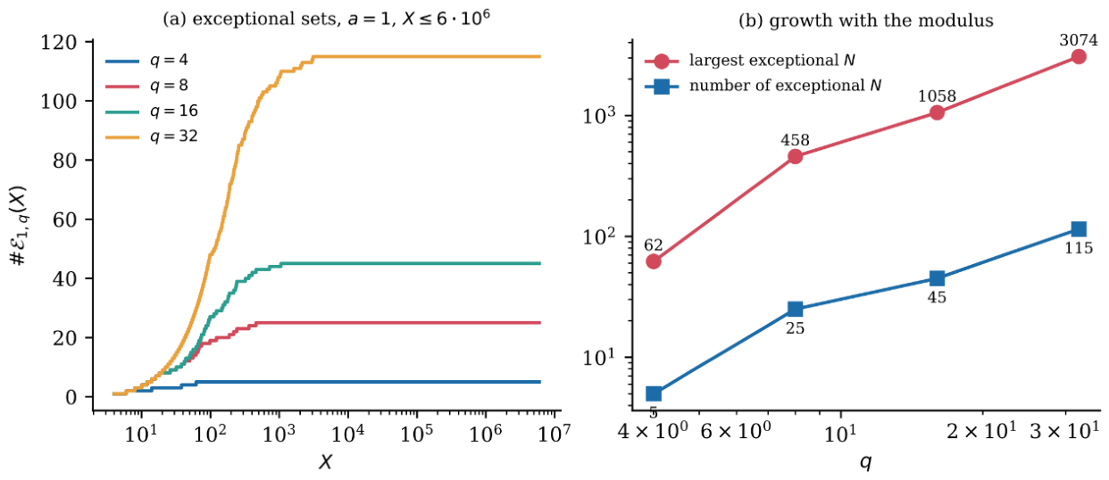

Table 1.
Ratio Ra,q(N)/Ma,q(N) over 120 random even N ∈ [5 ⋅ 106,107] [Comp. Verified].
| q | a | mean | s.d. | q | a | mean | s.d. |
| 3 | 1 | 0.9986 | 0.0029 | 9 | 4 | 0.9988 | 0.0046 |
| 3 | 2 | 0.9997 | 0.0027 | 10 | 3 | 0.9987 | 0.0044 |
| 5 | 2 | 0.9988 | 0.0042 | 12 | 5 | 0.9991 | 0.0040 |
| 6 | 1 | 0.9983 | 0.0029 | 15 | 7 | 0.9999 | 0.0048 |
| 6 | 5 | 0.9996 | 0.0027 | 30 | 7 | 0.9985 | 0.0042 |
| 7 | 3 | 1.0006 | 0.0059 |
Table 2.
Ray counts for n = 10 [Comp. Verified].
| X | π(X) | ray 1 | ray 3 | ray 7 | ray 9 |
| 103 | 168 | 40 | 42 | 46 | 38 |
| 104 | 1,229 | 306 | 310 | 308 | 303 |
| 105 | 9,592 | 2,387 | 2,402 | 2,411 | 2,390 |
| 106 | 78,498 | 19,617 | 19,665 | 19,621 | 19,593 |
| 107 | 664,579 | 166,104 | 166,230 | 166,211 | 166,032 |
| 108 | 5,761,455 | 1,440,298 | 1,440,474 | 1,440,495 | 1,440,186 |
Table 3.
Representability of Nn with p1≡1 (8); first K primes [Comp. Verified].
| K | pairs | representable | exceptions | fraction |
| 50 | 48 | 43 | 5 | 10.42% |
| 100 | 98 | 93 | 5 | 5.10% |
| 500 | 498 | 493 | 5 | 1.00% |
| 2000 | 1998 | 1993 | 5 | 0.25% |
| 5000 | 4998 | 4993 | 5 | 0.10% |
Table 4.
Primes p with R1,8(p + h) = 0, 11 ≤ p ≤ 6 ⋅ 106 − 20 [Comp. Verified].
| h | exceptions | largest exceptional p + h |
| −3 | 12 | 458 |
| −1 | 6 | 66 |
| 1 | 12 | 458 |
| 3 | 10 | 362 |
| 5 | 4 | 66 |
| 7 | 9 | 218 |
| 13 | 458 |
Table 5.
q = 3, a = 1: fraction of n with Nn≡1 (3) and with R1,3(Nn) = 0 [Comp. Verified].
| range of Nn | Nn≡1 (3) | R1,3(Nn) = 0 |
| [104,105) | 0.2070 | 0.1496 |
| [105,106) | 0.2069 | 0.1608 |
| [106,3 ⋅ 106) | 0.2127 | 0.1700 |
| [3 ⋅ 106,6 ⋅ 106) | 0.2152 | 0.1739 |
Table 6.
ℙ(ray(pn+1) = b∣ray(pn) = a), pairs below 108 [Comp. Verified].
| a∖b | 1 | 3 | 7 | 9 |
| 1 | 17.70% | 30.39% | 31.03% | 20.87% |
| 3 | 23.64% | 16.67% | 28.69% | 31.01% |
| 7 | 25.58% | 27.32% | 16.68% | 30.42% |
| 9 | 33.08% | 25.62% | 23.62% | 17.68% |
Table 7.
Mean gap gn by (ray of pn, ray of pn+1), pn+1 ≤ 2 ⋅ 107 [Comp. Verified].
| a∖b | 1 | 3 | 7 | 9 |
| 1 | 19.89 | 12.86 | 13.43 | 18.90 |
| 3 | 18.52 | 21.10 | 15.72 | 13.47 |
| 7 | 14.85 | 13.40 | 21.08 | 12.88 |
| 9 | 13.50 | 14.91 | 18.50 | 19.88 |
Table 8.
Gaps by size: share of all gaps and proportion keeping the ray, primes 5 < pn < pn+1 ≤ 108 [Comp. Verified].
Table 8.
Gaps by size: share of all gaps and proportion keeping the ray, primes 5 < pn < pn+1 ≤ 108 [Comp. Verified].
| gap gn | share of all gaps (%) | keeping the ray (%) |
| 2–8 | 34.43 | 0.00 |
| 10–18 | 32.32 | 23.09 |
| 20–38 | 24.54 | 30.12 |
| 40–58 | 6.50 | 23.58 |
| 60–98 | 2.10 | 36.28 |
| ≥100 | 0.12 | 28.29 |
Table 9.
Joint frequency of (pn mod 3,pn+1 mod 3) for consecutive primes 3 < pn < pn+1 ≤ N [Comp. Verified].
Table 9.
Joint frequency of (pn mod 3,pn+1 mod 3) for consecutive primes 3 < pn < pn+1 ≤ N [Comp. Verified].
| N | pairs | (1,1) | (1,2) = (2,1) | (2,2) |
| 3 ⋅ 106 | 216,813 | 21.21% | 28.76% | 21.27% |
| 107 | 664,576 | 21.50% | 28.48% | 21.53% |
| 108 | 5,761,452 | 21.94% | 28.06% | 21.95% |
| 109 | 50,847,531 | 22.25% | 27.74% | 22.26% |
Table 10.
Mod-3 joint frequencies against the prediction 1/4∓d(N); errors in percentage points [Comp. Verified].
Table 10.
Mod-3 joint frequencies against the prediction 1/4∓d(N); errors in percentage points [Comp. Verified].
| N | predicted diag. | predicted off-diag. | error vs. pred. | error vs. 25% | ratio |
| 3 ⋅ 106 | 22.74% | 27.26% | 1.4935 | 3.7584 | 0.397 |
| 107 | 22.84% | 27.16% | 1.3259 | 3.4818 | 0.381 |
| 108 | 23.02% | 26.98% | 1.0796 | 3.0566 | 0.353 |
| 109 | 23.17% | 26.83% | 0.9158 | 2.7442 | 0.334 |
Table 11.
Second moment of the error, q = 8, a = 1 [Comp. Verified].
| X | ||
| 2 × 10⁵ | 3.84 × 10⁻⁵ | 4.68 × 10⁻⁴ |
| 5 × 10⁵ | 1.83 × 10⁻⁵ | 2.41 × 10⁻⁴ |
| 106 | 1.00 × 10⁻⁵ | |
| 2 × 10⁶ | 5.65 × 10⁻⁶ | 8.20 × 10⁻⁵ |
| 3 × 10⁶ | 4.00 × 10⁻⁶ | 5.97 × 10⁻⁵ |
| 4.5 × 10⁶ | 2.67 × 10⁻⁶ | 4.09 × 10⁻⁵ |
| 6 × 10⁶ | 2.05 × 10⁻⁶ | 3.19 × 10⁻⁵ |
Table 12.
ℙ(Nn≡b (8)∣pn≡c (8)), Nn ≤ 6 ⋅ 106 [Comp. Verified].
| c∖b | 0 | 2 | 4 | 6 |
| 1 | 0.2838 | 0.1664 | 0.2842 | 0.2656 |
| 3 | 0.2868 | 0.2677 | 0.2799 | 0.1657 |
| 5 | 0.2846 | 0.1630 | 0.2863 | 0.2662 |
| 7 | 0.2849 | 0.2667 | 0.2848 | 0.1637 |
Table 13.
Recipe of Proposition 10.10 at four pairs (q,a); means in units of 10−5 [Comp. Verified].
| q | a | obs. | pred. | diff. (%) | z | spread obs./pred. | corr. |
| 8 | 1 | 10.79 | 11.05 | −2.4 | −4.0 | 1.80 / 1.43 | 0.993 |
| 16 | 1 | 19.77 | 20.19 | −2.1 | −3.5 | 3.28 / 3.22 | 0.962 |
| 16 | 9 | 19.42 | 20.02 | −3.0 | −5.1 | 1.93 / 1.87 | 0.958 |
| 32 | 1 | 38.60 | 39.53 | −2.4 | −4.1 | 6.50 / 6.81 | 0.940 |
Table 14.
Out-of-sample prediction of ρn+1 and gn/logpn from the last k rays modulo 10; test set pn > 5 ⋅ 107 [Comp. Verified].
Table 14.
Out-of-sample prediction of ρn+1 and gn/logpn from the last k rays modulo 10; test set pn > 5 ⋅ 107 [Comp. Verified].
| k | accuracy of ρn+1 | information gain (bits) | R2of gn/logpn |
| 1 | 0.3111 | 0.0330 | 0.00164 |
| 2 | 0.3152 | 0.0356 | 0.00178 |
| 3 | 0.3158 | 0.0360 | 0.00186 |
| 4 | 0.3160 | 0.0363 | 0.00187 |
| 5 | 0.3160 | 0.0361 | 0.00165 |
| 6 | 0.3144 | 0.0340 | 0.00062 |
Table 15.
Certified enclosures of Am(1) and Am(3) [Comp. Verified].
| m | Am(1)∈ | Am(3)∈ |
| 1 | [1.7427254016, 1.7427257501] | [1.1618169344, 1.1618171667] |
| 2 | [3.4607371607, 3.4607385450] | [1.3842948643, 1.3842954180] |
| 3 | [7.6303445889, 7.6303491671] | [1.6956321309, 1.6956331482] |
| 4 | [18.1823679115, 18.1823824574] | [2.1391021072, 2.1391038185] |
Disclaimer/Publisher’s Note: The statements, opinions and data contained in all publications are solely those of the individual author(s) and contributor(s) and not of MDPI and/or the editor(s). MDPI and/or the editor(s) disclaim responsibility for any injury to people or property resulting from any ideas, methods, instructions or products referred to in the content. |
© 2026 by the authors. Licensee MDPI, Basel, Switzerland. This article is an open access article distributed under the terms and conditions of the Creative Commons Attribution (CC BY) license (http://creativecommons.org/licenses/by/4.0/).
Copyright: This open access article is published under a Creative Commons CC BY 4.0 license, which permit the free download, distribution, and reuse, provided that the author and preprint are cited in any reuse.