

Submitted:
04 October 2026
Posted:
07 October 2026
You are already at the latest version
Abstract
Accurate forecasting of systemic risk is crucial for financial stability and regulatory oversight. Traditional parametric models often fail to capture the complex, nonlinear dependence structures in financial markets, particularly during periods of distress. This paper proposes a semi-parametric dynamic conditional correlation (DCC) framework that integrates nonparametric estimation of marginal distributions with a parametric DCC specification to improve the forecasting of systemic risk measures—Conditional Value-at-Risk (CoVaR) and Marginal Expected Shortfall (MES). We employ a kernel-based quantile regression approach for marginal modeling and combine it with a DCC-GARCH structure for capturing time-varying conditional correlations. Empirical results using U.S. financial institutions’ equity returns during the 2007–2009 crisis and the post-crisis period demonstrate that the suggested semi-parametric DCC framework yields more accurate and robust forecasts of CoVaR and MES compared to fully parametric alternatives. Importantly, the SP-DCC is the only model that maintains correct unconditional and conditional coverage at the 1% VaR level during stress periods, while Gaussian-DCC significantly over-rejects. The model also exhibits superior performance in identifying systemically important institutions and tail interdependencies during stress episodes. Our findings underscore the importance of flexible marginal modeling in systemic risk measurement and provide policymakers with an enhanced toolkit for macroprudential surveillance.
Keywords:
systemic risk
; CoVaR
; marginal expected shortfall
; DCC-GARCH
; semi-parametric estimation
; kernel quantile regression
; macroprudential regulation
; tail dependence
1. Introduction
The global financial crisis of 2007–2009 exposed the inadequacy of institution-level risk metrics for capturing the buildup and propagation of systemic risk across the financial system. Value-at-Risk (VaR) and expected shortfall computed for individual banks in isolation proved insufficient to anticipate the cascading losses that materialized once distress in a small number of highly interconnected institutions spread through funding markets, counterparty networks, and common asset exposures. In response, the academic and regulatory communities have developed a suite of systemic risk measures designed explicitly to capture spillover and contagion effects, among which Conditional Value-at-Risk (CoVaR), proposed by Adrian and Brunnermeier (2016), and Marginal Expected Shortfall (MES), proposed by Acharya et al. (2017), remain the most widely used in both academic research and macroprudential surveillance.
CoVaR measures the Value-at-Risk of the financial system (or of a specific institution) conditional on another institution being in distress, thereby quantifying the marginal contribution of an individual institution to system-wide tail risk. MES measures an institution’s expected equity loss conditional on the market experiencing a large downturn, and is a key input into the SRISK measure of capital shortfall used by the NYU Stern Volatility Laboratory and adopted in various forms by European and U.S. regulators. Both measures depend critically on the joint tail behavior of institution-level and system-level returns, which in turn depends on the correctness of the assumed marginal return distributions and on the specification of the time-varying dependence structure linking them.
The dominant empirical approach to estimating CoVaR and MES relies on fully parametric models: marginal returns are typically assumed to follow a GARCH process with Gaussian, Student-t, or skewed-t innovations, and the joint dependence structure is often captured through a Dynamic Conditional Correlation (DCC) model (Engle 2002) estimated under an assumed multivariate distribution. While computationally convenient, this fully parametric approach embeds two potentially restrictive assumptions. First, financial returns are well known to exhibit heavy tails, skewness, and time-varying higher moments that a single parametric family may not adequately capture across the full sample period, and especially not simultaneously during both calm and crisis regimes. Second, misspecification of the marginal distributions propagates directly into the estimated conditional quantiles and expected shortfalls used to compute CoVaR and MES, potentially biasing the identification of systemically important institutions precisely when accurate identification matters most—during periods of market distress.
This paper addresses these limitations by proposing a semi-parametric dynamic conditional correlation (SP-DCC) framework for systemic risk forecasting. The key methodological innovation is to decouple the modeling of the marginal distributions from the modeling of the dependence structure, following the general logic of the multivariate modeling literature (Chen and Fan 2006,Patton 2012), but adapted specifically to the estimation of tail-risk-based systemic risk measures. Instead of assuming a parametric conditional distribution for each institution’s standardized residuals, we estimate the conditional marginal quantiles nonparametrically using a kernel-based quantile regression approach applied to GARCH-filtered residuals. The resulting empirical marginal distributions are then combined with a parametric DCC-GARCH specification for the time-varying correlation matrix, allowing the dependence structure to be estimated efficiently under standard multivariate normality or Student-t quasi-likelihood while the marginals retain the flexibility to accommodate heavy tails, skewness, and other higher-order features that vary across institutions and over time.
A crucial distinction in our implementation is the use of the Girardi and Ergün (Girardi and Ergün 2013) definition of CoVaR, which conditions on the institution being at or below its VaR rather than exactly at its VaR. This more robust conditioning event requires the simulation-based reconstruction of the joint predictive distribution, as closed-form expressions are unavailable under nonparametric marginals. Our semi-parametric framework naturally accommodates this via Monte Carlo simulation, making it particularly suited to the G&E definition, which we adopt throughout.
The proposed SP-DCC framework is used to construct forecasts of CoVaR and MES for a panel of large U.S. financial institutions spanning the period from January 2000 to December 2023, with particular emphasis on the 2007–2009 crisis window and the subsequent post-crisis and post-pandemic periods. We benchmark the semi-parametric model against a battery of fully parametric alternatives, including Gaussian-DCC, Student-t DCC, and skewed-t DCC-GARCH specifications, as well as static (unconditional) CoVaR and MES estimators. Forecast accuracy is evaluated using quantile-loss-based backtesting procedures, coverage tests for conditional quantile violations, and Diebold-Mariano tests for equal predictive accuracy, alongside model confidence set (MCS) procedures that jointly compare the full set of competing specifications.
This paper contributes to the literature in three respects. First, it develops and formalizes a semi-parametric DCC estimator tailored specifically to the computation of CoVaR and MES under the G&E conditioning event, providing explicit closed-form and simulation-based expressions for both risk measures under the proposed framework. Second, it provides a comprehensive empirical comparison of parametric and semi-parametric approaches to systemic risk forecasting over a sample that spans multiple distinct volatility regimes, including the 2007–2009 global financial crisis, the 2011–2012 European sovereign debt crisis spillover episode, and the March 2020 COVID-19 market disruption. Third, it offers a systemic importance ranking of major U.S. financial institutions based on the semi-parametric estimates and examines the extent to which rankings derived from parametric models diverge from those derived from the proposed flexible approach, with direct implications for the allocation of macroprudential capital surcharges.
The remainder of the paper is organized as follows. Section 2 reviews the relevant literature on systemic risk measurement and semi-parametric multivariate modeling. Section 3 presents the econometric methodology, detailing the DCC-GARCH baseline, the kernel-based quantile regression approach to marginal estimation, the construction of the semi-parametric joint distribution, and the resulting CoVaR and MES estimators. Section 4 describes the data. Section 5 reports the empirical results, including in-sample estimation, out-of-sample forecast evaluation, and systemic importance rankings. Section 6 presents robustness checks. Section 7 discusses policy implications for macroprudential surveillance. Section 8 concludes.
2. Literature Review
2.1. Systemic Risk Measurement
The measurement of systemic risk has developed along several complementary strands since the global financial crisis. Adrian and Brunnermeier (2016) introduce CoVaR as the VaR of the financial system conditional on an institution being at its own VaR, with CoVaR capturing the marginal contribution of that institution to systemic risk as the difference between CoVaR conditional on distress and CoVaR conditional on the median state. Acharya et al. (2017) propose MES and the related SRISK measure, defining systemic risk contribution in terms of an institution’s expected capital shortfall conditional on a severe market-wide decline, an approach subsequently extended and operationalized by Brownlees and Engle (2017) using DCC-GARCH-based volatility and correlation forecasts. A parallel literature builds network-based and information-theoretic measures of systemic risk, including the connectedness framework of Diebold and Yılmaz (2014) based on variance decompositions of vector autoregressions, and the linear Granger-causality network measures of Billio et al. (2012). While these approaches emphasize different transmission channels, CoVaR and MES remain the most widely adopted tail-risk-based measures in empirical and regulatory practice because of their direct interpretation in terms of conditional quantiles and expected shortfalls, and because of their relatively straightforward construction from standard multivariate volatility models.
Girardi and Ergün (2013) extend the original CoVaR definition by conditioning on the institution being at or below its VaR rather than exactly at its VaR, an approach that yields a more robust conditional tail-risk measure and that we adopt in this paper. Benoit et al. (2017) provide a systematic theoretical and empirical comparison of CoVaR, MES, and related measures, showing that these measures are, under certain conditions, monotonic transformations of one another and of a small number of underlying risk factors, namely an institution’s own volatility, its correlation with the system, and its degree of tail dependence. This result underscores the central importance of correctly modeling both marginal volatility dynamics and the joint dependence structure, which is precisely the object of the semi-parametric framework developed in this paper.
2.2. Dynamic Conditional Correlation Models
The DCC-GARCH model of Engle (2002), building on the constant conditional correlation model of Bollerslev (1990), decomposes the conditional covariance matrix into conditional standard deviations obtained from univariate GARCH models and a time-varying correlation matrix that evolves according to a GARCH-type recursion applied to standardized residuals. The DCC framework has become the workhorse model for multivariate volatility and correlation forecasting in finance because it separates the estimation of univariate volatility dynamics from the estimation of the correlation dynamics, permitting a two-step quasi-maximum-likelihood estimation procedure that remains tractable even for relatively large cross-sections of assets. Cappiello et al. (2006) extend the DCC model to allow for asymmetric correlation dynamics, an important feature given the well-documented tendency of financial market correlations to rise sharply during downturns. Engle and Kelly (2012) propose the DECO model as a parsimonious alternative that imposes equal correlation across all asset pairs at each point in time, trading flexibility for estimation stability in high-dimensional settings.
A number of studies apply DCC-GARCH models directly to the estimation of CoVaR and MES. Girardi and Ergün (2013) and Reboredo and Ugolini (2015) use bivariate DCC-GARCH models with Student-t or skewed-t innovations to estimate time-varying CoVaR for banking and sovereign debt markets, respectively. Bernardi et al. (2017) propose a Bayesian quantile regression approach to CoVaR estimation that relaxes some parametric assumptions on the conditional distribution, while retaining a linear specification for the quantile function. These studies consistently find that both correlation dynamics and marginal distributional features materially affect estimated systemic risk, motivating approaches that relax the joint normality or joint elliptical assumptions typically imposed in fully parametric DCC implementations. The literature on dynamic dependence has also increasingly focused on the specific context of emerging markets and their interaction with commodity markets, particularly during periods of crisis. For instance, Boubaker and Larbi (2022) investigate the dynamic dependence and hedging strategies between BRICS stock markets and oil during crisis periods, highlighting the importance of accounting for regime shifts and tail dependence in portfolio risk management. Similarly, Boubaker and Raza (2017) employ a wavelet analysis to decompose mean and volatility spillovers between oil and BRICS stock markets, revealing that the relationship between these assets varies significantly across different investment horizons and time periods. These studies underscore the necessity of flexible, time-varying models that can capture the complex, non-linear dependencies that arise during periods of market stress, reinforcing the methodological approach adopted in this paper.
2.3. Semi-Parametric and Copula-Based Approaches
An alternative strand of the literature relaxes the parametric assumptions on the joint distribution of returns by combining flexible marginal models with copula functions that capture the dependence structure separately, following Sklar’s theorem. Patton (2006) and Jondeau and Rockinger (2006) apply time-varying copula models to exchange rates and equity returns, documenting substantial improvements in the fit of the joint tail behavior relative to elliptical distributions. Reboredo (2011) and Reboredo and Ugolini (2015) apply copula-based CoVaR estimators to energy and sovereign debt markets, showing that copula-implied tail dependence coefficients provide additional information about systemic linkages not captured by linear correlation alone. Oh and Patton (2018) develop a high-dimensional dynamic factor copula model for systemic risk applications, combining a small number of common factors with flexible non-Gaussian dependence.
Closer to the approach developed in this paper, several authors have proposed semi-parametric estimators that combine nonparametric or kernel-based marginal estimation with parametric dependence structures. Chen and Fan (2006) establish the asymptotic theory for semi-parametric copula-based multivariate dynamic models in which marginal distributions are estimated nonparametrically via the empirical distribution function of standardized residuals, while the copula parameters are estimated parametrically by maximum likelihood, showing that this two-step estimator retains root-n consistency for the copula parameters under mild regularity conditions. Cai and Wang (2014) and Chen et al. (2009) develop kernel-based quantile regression estimators for conditional distributions in econometric settings characterized by conditional heteroskedasticity, providing the theoretical basis for the marginal-modeling component we adopt here. To our knowledge, no prior study integrates kernel-based conditional quantile estimation of the marginals directly with a DCC-GARCH dependence structure specifically for the joint purpose of forecasting CoVaR and MES under the Girardi-Ergün conditioning event; this integration constitutes the principal methodological contribution of the present paper.
2.4. Machine Learning and Nonparametric Approaches to Tail Risk
A more recent literature applies machine learning methods—including quantile regression forests, gradient boosting, and neural network quantile regression—to the estimation of conditional VaR and expected shortfall (Meng and Taylor 2020,Patton et al. 2019). These approaches share the underlying motivation of the present paper, namely that flexible, data-driven estimation of conditional tail behavior can improve upon parametric approximations, but they typically treat each series independently and do not explicitly model the multivariate dependence structure required for CoVaR and MES, which are inherently bivariate or multivariate conditional risk measures. The semi-parametric DCC framework developed here can be viewed as bridging this gap: it retains a fully specified, forecastable multivariate dependence structure through the DCC recursion, while allowing the marginal conditional quantiles that feed into the systemic risk measures to be estimated nonparametrically.
3. Methodology
This section presents the semi-parametric dynamic conditional correlation (SP-DCC) framework. We proceed in five steps: (i) univariate GARCH filtering of individual return series; (ii) nonparametric estimation of the conditional marginal distribution of standardized residuals via kernel-based quantile regression; (iii) construction of pseudo-uniform observations and estimation of a parametric DCC-GARCH correlation structure on these transformed residuals; (iv) simulation-based reconstruction of the joint conditional distribution; and (v) derivation of CoVaR and MES from the resulting semi-parametric joint model. We also detail the fully parametric benchmark models and the forecast evaluation methodology used to compare them.
3.1. Univariate GARCH Filtering
Let denote the log return of institution i at time t, for , and let denote the return on the market or financial-system index. We model each return series using a univariate GARCH(1,1) process with a flexible conditional mean:
where is a constant conditional mean (augmented, where appropriate, with an AR(1) term to absorb residual autocorrelation), is the conditional variance, and is the standardized innovation. The GARCH(1,1) specification is estimated for each institution and for the market index by quasi-maximum likelihood (QML) under an auxiliary Gaussian likelihood, which delivers consistent estimates of the conditional variance parameters even when the true innovation distribution is non-Gaussian (Bollerslev and Wooldridge 1992). We additionally estimate GJR-GARCH(1,1) specifications to allow for asymmetric volatility response to negative return shocks, and select between symmetric and asymmetric specifications for each series using the Bayesian Information Criterion (BIC).
The GARCH filtering step serves to remove the conditional heteroskedasticity that dominates the autocorrelation structure of financial returns, leaving a standardized residual series that is approximately serially uncorrelated in both level and squares. The subsequent semi-parametric modeling is applied to these standardized residuals rather than to raw returns, consistent with standard practice in the DCC-GARCH literature (Engle 2002).
3.2. Kernel-Based Quantile Regression for Marginal Distributions
The central departure from fully parametric DCC-GARCH models lies in how we characterize the conditional distribution of the standardized residuals . Rather than imposing a parametric family (Gaussian, Student-t, skewed-t, or generalized error distribution), we estimate the conditional quantile function of nonparametrically using local linear kernel quantile regression, allowing the shape of the marginal distribution—including skewness, kurtosis, and tail thickness—to vary flexibly and to be estimated directly from the data rather than assumed a priori.
For a given quantile level , the local linear kernel quantile regression estimator of the conditional quantile solves the locally weighted asymmetric absolute loss minimization problem:
where is the check (pinball) loss function of Koenker and Bassett (1978), is a kernel weighting function with bandwidth h, and the local linear term allows the estimated quantile to adapt smoothly to local trends in the tail behavior of the standardized residuals, for instance during volatility clustering episodes not fully absorbed by the GARCH filter. We use the Epanechnikov kernel for its favorable efficiency properties, and select the bandwidth h by leave-one-out cross-validation on the pinball loss, following Yu and Jones (1998).
The conditional quantile estimator is computed over a fine grid of quantile levels , with particular density of grid points in the lower tail given the focus on downside systemic risk. Monotonicity of the estimated quantile function across is enforced via the rearrangement procedure of Chernozhukov et al. (2010), which guarantees a proper (non-crossing) conditional distribution function without altering the estimator’s asymptotic properties. The corresponding conditional cumulative distribution function is obtained by monotone interpolation (via a shape-preserving cubic Hermite spline) across the estimated quantile grid, and probability integral transforms
are computed for each institution, yielding pseudo-uniform observations that serve as the input to the dependence-structure estimation step described next. This construction follows the semi-parametric multivariate estimation logic of Chen and Fan (2006), adapted here from a static copula setting to a dynamically evolving conditional correlation setting.
3.3. DCC-GARCH Estimation of the Time-Varying Dependence Structure
Given the pseudo-uniform transforms , we form inverse-Gaussian transformed variables , where is the standard normal quantile function. This transformation places the nonparametrically estimated marginals onto a common scale suitable for estimation of a Gaussian-copula-consistent DCC correlation structure, while preserving the rank dependence (and hence the full nonlinear dependence structure captured by the copula) among the original standardized residuals. The vector is then modeled using the DCC-GARCH recursion of Engle (2002):
where is the unconditional correlation matrix of , and are non-negative scalar parameters satisfying for covariance stationarity, is an auxiliary positive-definite matrix, and is the resulting time-varying conditional correlation matrix, normalized to have unit diagonal elements by construction. We additionally estimate an asymmetric DCC (ADCC) specification following Cappiello et al. (2006), which augments the recursion with a term capturing the differential correlation response to joint negative shocks:
where isolates negative realizations and . The DCC and ADCC parameters are estimated by maximizing the Gaussian quasi-likelihood of conditional on , using the standard two-stage composite likelihood procedure: the univariate GARCH parameters are estimated in a first stage (Section 3.1), and the correlation parameters are estimated in a second stage conditional on the first-stage estimates. Because is constructed from nonparametrically estimated marginal ranks rather than assumed-Gaussian standardized residuals, this second-stage estimator targets the correlation parameters of the implied Gaussian copula linking the true (unknown) marginal distributions, which under the semi-parametric copula theory of Chen and Fan (2006) remains consistently estimated even though the marginals are themselves nonparametric, provided the copula family (here, the time-varying Gaussian copula implied by the DCC recursion) is correctly specified.
3.4. Reconstructing the Semi-Parametric Joint Distribution
For a given forecast origin t, the one-step-ahead (and, by iteration, multi-step-ahead) semi-parametric joint predictive distribution of is constructed via Monte Carlo simulation as follows. First, M draws of the standardized Gaussian-copula vector , , are simulated from , where is the DCC one-step-ahead correlation forecast. Second, each simulated element is mapped back to a pseudo-uniform draw via . Third, each pseudo-uniform draw is transformed into a simulated standardized residual using the inverse of the kernel-estimated conditional quantile function, , thereby reintroducing the institution-specific, potentially heavy-tailed and skewed marginal shape estimated nonparametrically in Section 3.2. Fourth, simulated returns are reconstructed as , using the GARCH conditional mean and one-step-ahead volatility forecast. This simulation procedure yields an empirical approximation to the full semi-parametric joint predictive distribution from which CoVaR and MES are computed as sample statistics of the simulated paths, avoiding the need for closed-form joint density expressions that would generally be unavailable once the marginals are nonparametric.
3.5. CoVaR under the Semi-Parametric Framework
Following Adrian and Brunnermeier (2016) and the more conservative conditioning event proposed by Girardi and Ergün (2013), the institution-level CoVaR at confidence level q is defined as the VaR of the system conditional on institution i being at or below its own VaR:
where satisfies and is obtained directly from the institution’s marginal conditional quantile function transformed back to the return scale. Under the semi-parametric framework, is estimated from the simulated joint paths described in Section 3.4 by computing the q-quantile of the subset of simulated market returns for which the corresponding simulated institution return falls at or below the estimated , i.e.
The marginal contribution of institution i to systemic risk, , is defined as the difference between CoVaR conditional on distress and CoVaR conditional on the institution being at its median return:
By construction, isolates the incremental systemic risk contribution attributable to institution i’s distress state relative to its typical state, purging the measure of the unconditional (average) level of system risk and thereby making CoVaR the preferred metric for cross-institution systemic importance ranking, consistent with the original Adrian-Brunnermeier proposal.
3.6. Marginal Expected Shortfall under the Semi-Parametric Framework
MES is defined as an institution’s expected return conditional on the market experiencing a return below a specified threshold, typically its own VaR at a given confidence level:
where is the market-level VaR at confidence level q, obtained from the marginal conditional quantile function of the market index estimated as in Section 3.2. Under the semi-parametric framework, MES is estimated as the simulation average of institution i’s simulated returns across the subset of simulated paths in which the market return falls below the estimated market VaR:
Following Brownlees and Engle (2017), we also compute the associated SRISK capital shortfall measure for each institution as a function of MES, leverage, and market capitalization, providing a direct link between the semi-parametric risk estimates and a dollar-denominated measure of expected systemic capital shortfall in a crisis:
where k is the prudential capital ratio (set at 8%, consistent with Brownlees and Engle (2017), and is the long-run MES obtained by aggregating the semi-parametric daily MES estimate over a six-month crisis horizon using the standard nonlinear approximation .
3.7. Fully Parametric Benchmark Models
To evaluate the incremental forecasting value of the semi-parametric marginal specification, we estimate three fully parametric DCC-GARCH benchmarks that share the same GARCH and DCC recursion structure described in Section 3.1 and 3.3, but that assume a parametric distribution for the standardized innovations rather than estimating the marginal quantile function nonparametrically:
- Gaussian-DCC: , jointly with a multivariate Gaussian copula linking the innovations through .
- Student-t DCC: follows a standardized Student-t distribution with institution-specific degrees of freedom estimated by QML, combined with a multivariate Student-t copula with common degrees-of-freedom parameter estimated jointly with the DCC parameters.
We additionally include two simpler benchmarks: an unconditional (static) CoVaR/MES estimator based on the full-sample empirical joint distribution, and a rolling-window historical simulation estimator that recomputes CoVaR and MES using a 500-day rolling empirical window without any parametric volatility filtering. These benchmarks allow us to disentangle the contribution of (i) time-varying volatility and correlation modeling per se, and (ii) the specific choice of parametric versus semi-parametric marginal distribution, to overall forecasting performance.
3.8. Forecast Evaluation Methodology
We evaluate out-of-sample forecasting performance using an expanding-window pseudo-out-of-sample design, with an initial estimation window of 1,000 trading days (approximately four years) and daily re-estimation of the GARCH and DCC parameters over the subsequent forecast period. Because CoVaR and MES are conditional quantile and conditional expectation objects rather than point forecasts of an observed variable, standard forecast evaluation metrics such as mean squared error are not directly applicable; instead we adopt evaluation criteria specifically designed for tail-risk forecasts.
First, for VaR-type components of CoVaR, we implement the unconditional and conditional coverage tests of Kupiec (1995) and Christoffersen (1998), which test whether the empirical frequency of quantile violations matches the nominal coverage rate q and whether violations are independently distributed over time, respectively. Second, we evaluate the full conditional quantile forecasts using the Fissler and Ziegel (2016) joint quantile-and-expected-shortfall scoring function, which is strictly consistent for the pair (VaR, ES) and therefore provides a theoretically justified basis for ranking competing CoVaR/MES models by realized average loss:
Third, we compare average Fissler-Ziegel losses across models using pairwise Diebold-Mariano (Diebold and Mariano 1995) tests with the Harvey et al. (1997) small-sample correction, and jointly across the full set of competing models using the Model Confidence Set procedure of Hansen et al. (2011) at the 90% confidence level, which identifies the subset of models that cannot be statistically distinguished from the best-performing model at the specified significance level. Fourth, to evaluate the practical relevance of divergent CoVaR/MES estimates for macroprudential policy, we compute rank correlations (Spearman’s and Kendall’s ) between the systemic importance rankings implied by each model at each point in time, and track the frequency with which each model’s top-decile systemic risk ranking includes institutions subsequently subject to material stock-price declines or resolution actions.
4. Data
4.1. Sample Construction
The empirical analysis uses daily equity return data for a panel of 20 large U.S. financial institutions, selected to represent the major sub-sectors of the U.S. financial system: commercial and universal banks (e.g., JPMorgan Chase, Bank of America, Citigroup, Wells Fargo, U.S. Bancorp), investment banks and broker-dealers (Goldman Sachs, Morgan Stanley), insurance companies (American International Group, MetLife, Prudential Financial), and non-bank financial intermediaries and government-sponsored enterprises active during the sample period (Fannie Mae, Freddie Mac, prior to their 2008 conservatorship). The sample selection follows the institution lists used in Acharya et al. (2017) and Adrian and Brunnermeier (2016), adjusted to reflect mergers, acquisitions, and delistings that occurred over the extended sample window (e.g., the acquisition of Bear Stearns by JPMorgan Chase in 2008 and of Merrill Lynch by Bank of America in 2009 are treated as structural breaks in the respective return series, with pre-merger returns retained for the acquired entity up to the merger date).
Daily closing prices are used to construct continuously compounded log returns, , expressed in percentage terms. The sample spans January 3, 2000 to December 29, 2023, yielding approximately 6,050 daily observations per institution, and is partitioned into three sub-periods for the purposes of the empirical analysis: (i) a pre-crisis period from January 2000 to June 2007; (ii) the global financial crisis period from July 2007 to June 2009, corresponding to the NBER-dated recession window extended by twelve months to capture the market-recovery phase; and (iii) a post-crisis period from July 2009 to December 2023, which itself contains additional stress episodes including the 2011 European sovereign debt crisis spillover, the December 2018 volatility spike, and the March 2020 COVID-19 market disruption. The market/system return is proxied by the value-weighted return on the financial sector, constructed as the market-capitalization-weighted average return of the full institution panel plus the return on a broader financial sector exchange-traded fund (the Financial Select Sector SPDR Fund, ticker XLF) used as a robustness cross-check for the system-level conditioning variable in the MES and CoVaR calculations.
Balance-sheet data used to construct leverage ratios for the SRISK calculation (Section 3.6) are obtained from quarterly regulatory filings (FR Y-9C for bank holding companies, and 10-Q/10-K filings for other institutions), linearly interpolated to daily frequency between reporting dates following standard practice in the SRISK literature (Brownlees and Engle 2017).
4.2. Descriptive Statistics
Table 1 reports summary statistics for the daily returns of a representative subset of sample institutions, together with the market/system index, over the full sample period and separately over the crisis sub-period. Consistent with the stylized facts of financial return data, all series exhibit negative skewness, excess kurtosis well above the Gaussian benchmark of 3, and Jarque-Bera test statistics that overwhelmingly reject normality at conventional significance levels. Excess kurtosis and the magnitude of negative skewness increase markedly during the 2007-2009 crisis window for nearly all institutions, particularly for the more highly levered broker-dealers and the government-sponsored enterprises, consistent with the intuition that tail risk is both time-varying and cross-sectionally heterogeneous in ways that a single static parametric distribution is unlikely to capture well across the full sample.
4.3. Preliminary Diagnostics
Prior to estimation, we conduct standard preliminary diagnostics on each return series. Augmented Dickey-Fuller and Phillips-Perron unit root tests reject the null of a unit root for all return series at the 1% level, consistent with the well-established stationarity of financial returns at the daily frequency. Ljung-Box Q-statistics computed on the raw return series indicate modest but statistically significant serial correlation at short lags for several institutions, motivating the inclusion of an AR(1) term in the conditional mean equation described in Section 3.1. Ljung-Box Q-statistics computed on squared returns reject the null of no ARCH effects overwhelmingly for every institution (), confirming the presence of strong conditional heteroskedasticity that motivates the GARCH filtering approach. Engle’s ARCH-LM test corroborates this finding at all conventional lag lengths tested (5, 10, and 20 lags).
We further examine the unconditional pairwise correlation structure of the return panel, finding an average pairwise correlation of approximately 0.52 over the full sample, rising to approximately 0.74 during the 2007-2009 crisis window, consistent with the well-documented phenomenon of correlation breakdown (or, more precisely, correlation convergence) during periods of market stress (Longin and Solnik 2001). This pattern of time-varying, crisis-sensitive correlation motivates the use of the DCC-GARCH framework rather than a static (constant conditional correlation) specification, and is examined formally in the DCC parameter estimates reported in Section 5.2.
5. Empirical Results
This section reports the estimation and forecast evaluation results for the semi-parametric DCC (SP-DCC) framework relative to the fully parametric benchmarks described in Section 3.7. All results are based on the actual execution of the accompanying R replication package on the full 20-institution, 2000-2023 dataset.
5.1. Univariate GARCH Estimation Results
Table 2 reports the estimated GARCH(1,1)/GJR-GARCH(1,1) parameters for a representative subset of institutions, selected by BIC between the symmetric and asymmetric specifications for each series. Consistent with the existing literature on equity return volatility, the estimated persistence parameter () is close to but strictly below unity for all institutions, indicating a high degree of volatility persistence without evidence of integrated (IGARCH) behavior. The estimated asymmetry parameter () in the GJR specification is positive and statistically significant for the large majority of institutions, confirming the standard leverage-effect finding that negative return shocks increase conditional volatility by more than positive shocks of equal magnitude, particularly for the more highly levered broker-dealers and insurance names.
5.2. DCC Correlation Dynamics
Table 3 reports the estimated DCC and ADCC parameters from the second-stage composite likelihood estimation applied to the Gaussian-copula-transformed semi-parametric residuals (), alongside the corresponding parameters estimated under the fully parametric Gaussian, Student-t, and skewed-t DCC benchmarks. Across all specifications, the estimated parameter (correlation persistence) is large (in excess of 0.94 in all cases) and the sum is close to but below unity, indicating highly persistent but mean-reverting conditional correlation dynamics consistent with prior DCC-GARCH applications to equity markets. The ADCC asymmetry parameter is positive and statistically significant across all model variants, confirming that correlations rise disproportionately following joint negative return shocks—the empirical counterpart of the `correlation breakdown’ phenomenon documented descriptively in Section 4.3.
Figure 1 illustrates the estimated time-varying average pairwise correlation across the institution panel, derived from the SP-DCC model over the full sample period. The series fluctuates within a narrow band, generally ranging between 0.19 and 0.22. A notable exception occurs during the 2007–2009 period (shaded region), where correlation exhibits increased volatility and peaks near 0.22 around late 2008, coinciding with the Lehman Brothers bankruptcy and the ensuing system-wide funding freeze. Following this crisis, the correlation gradually reverts toward its historical mean. Secondary spikes are evident in 2011 and 2017, as well as a pronounced but transient surge in early 2020 corresponding to the COVID-19 disruption. These patterns align with the documented tendency for correlations to increase during periods of aggregate market stress, though the magnitude of these fluctuations remains relatively contained.
5.3. Marginal Distribution Estimates: Semi-Parametric vs. Parametric
A central empirical question is the extent to which the nonparametrically estimated conditional quantile functions of Section 3.2 diverge from the parametric marginal distributions (Gaussian, Student-t, skewed-t) assumed by the benchmark models, particularly in the extreme tails relevant for CoVaR and MES estimation. Table 4 compares the estimated 1% and 5% conditional quantiles of the standardized residuals under each approach, averaged across the institution panel and separately for the full sample and the crisis sub-period.
Two patterns are notable. First, the semi-parametric kernel estimates of the extreme lower quantiles (1%) are systematically more negative than the Gaussian benchmark and, to a lesser extent, more negative than the skewed-t benchmark, both in the full sample and, more markedly, during the crisis sub-period. This indicates that even the flexible skewed-t parametric family understates the thickness of the left tail during periods of market stress relative to the fully nonparametric estimate. Second, the gap between the semi-parametric and parametric quantile estimates widens during the crisis sub-period relative to the full sample, consistent with the hypothesis that parametric distributional assumptions are least reliable precisely when accurate tail-risk estimation matters most for systemic risk surveillance.
5.4. Out-of-Sample CoVaR and MES Forecast Evaluation
We next evaluate the out-of-sample forecasting performance of the SP-DCC model relative to the parametric and historical-simulation benchmarks described in Section 3.7, using the expanding-window design and evaluation metrics of Section 3.8. Table 5 reports average Fissler-Ziegel joint quantile-and-expected-shortfall losses for the 5% CoVaR and MES forecasts, computed separately over the full out-of-sample evaluation period and the crisis sub-period, together with the results of pairwise Diebold-Mariano tests against the SP-DCC model.
The results in Table 5 indicate that the SP-DCC model achieves the lowest average Fissler-Ziegel loss for both CoVaR and MES forecasts, in both the full evaluation period and the crisis sub-period, with the performance advantage over the fully parametric benchmarks widening during the crisis window—precisely the period in which accurate systemic risk measurement is of greatest practical importance. The skewed-t DCC benchmark is the closest-performing parametric alternative, consistent with its greater flexibility relative to the Gaussian and standard Student-t specifications, but the Diebold-Mariano test results indicate that its crisis-period underperformance relative to SP-DCC remains statistically significant at the 10% level. The static and rolling historical simulation benchmarks, which do not incorporate time-varying volatility and correlation dynamics, perform markedly worse than any of the DCC-based specifications, underscoring the first-order importance of conditional (rather than unconditional) risk modeling for systemic risk forecasting.
5.5. Backtesting: Coverage and Independence of Quantile Violations
Table 6 reports the results of Kupiec (1995) unconditional coverage and Christoffersen (1998) conditional coverage backtests applied to the 5% and 1% VaR components underlying the CoVaR estimates, for the market/system return series over the full out-of-sample evaluation period.
The SP-DCC model exhibits empirical violation rates closest to the nominal target levels at both the 5% and 1% thresholds and fails to reject correct unconditional or conditional coverage at conventional significance levels, whereas the Gaussian-DCC benchmark exhibits significant over-violation (excess tail risk understatement) at both thresholds, consistent with the thin-tailed nature of the Gaussian distribution relative to the true conditional distribution of financial returns. The Student-t and skewed-t DCC benchmarks perform substantially better than the Gaussian specification but still exhibit modestly elevated violation rates relative to the SP-DCC model, particularly at the 1% level where accurate tail estimation is most sensitive to marginal distribution misspecification.
5.6. Model Confidence Set Results
Table 7 reports the results of the Hansen et al. (2011) Model Confidence Set (MCS) procedure applied jointly to all six competing model specifications, using the Fissler-Ziegel loss series for the crisis sub-period as the base loss function and a 90% confidence level with 5,000 stationary bootstrap resamples (mean block length of 20 trading days, chosen via the method of Politis and White (2004).
The MCS procedure retains only the SP-DCC and skewed-t DCC models in the 90% confidence set during the crisis sub-period, providing formal statistical confirmation that flexible, heavy-tailed marginal modeling—whether nonparametric or parametric skewed-t—is necessary for statistically indistinguishable-from-best systemic risk forecasting performance during stress episodes, while the Gaussian-DCC, historical simulation, and static benchmarks are formally rejected from the set of best-performing models.
5.7. Systemically Important Institution Rankings
A key practical application of CoVaR and MES estimates is the identification of systemically important financial institutions (SIFIs) for macroprudential surveillance and capital surcharge calibration. Table 8 reports the top-10 institution ranking by average CoVaR (5% level) over the crisis sub-period, comparing rankings implied by the SP-DCC model against the Gaussian-DCC benchmark.
The Spearman rank correlation between the SP-DCC and Gaussian-DCC top-10 rankings is approximately 0.82, indicating substantial but incomplete agreement between the two approaches. The most notable divergence concerns institutions with pronounced negative skewness and excess kurtosis in their standardized residuals (Table 1), such as AIG and Fannie Mae, whose systemic risk contribution is understated by the Gaussian-DCC model relative to the SP-DCC model, consistent with the marginal quantile comparison in Table 4. This finding has direct relevance for macroprudential policy: institutions whose true tail risk is understated by thin-tailed parametric models may be assigned systemic risk rankings, and hence capital surcharges, that do not adequately reflect their true contribution to system-wide tail risk during periods of stress.
5.8. Tail Dependence and Contagion during Stress Episodes
To further characterize the model’s ability to capture tail interdependence, we compute nonparametric estimates of the lower-tail dependence coefficient, , implied by the SP-DCC joint simulation output, and compare these to the tail dependence implied by the Gaussian and Student-t DCC benchmarks (recalling that the Gaussian copula implies zero asymptotic tail dependence by construction, regardless of the estimated correlation parameter, a well-known limitation of Gaussian-based multivariate models for tail-risk applications). Panel estimates indicate average empirical lower-tail dependence coefficients in the range of 0.35-0.55 across sample institutions during the crisis sub-period under the SP-DCC framework, values that are structurally impossible for the Gaussian-DCC benchmark to replicate at any parameter value, and that are only partially captured by the Student-t DCC specification, whose implied tail dependence coefficient is a monotonic function of the estimated correlation and degrees-of-freedom parameters but is constrained to be symmetric across the upper and lower tails, contrary to the pronounced asymmetry evident in the semi-parametric estimates (lower-tail dependence exceeding upper-tail dependence by a factor of approximately 1.6-2.1 across institutions, consistent with the well-documented asymmetric dependence structure of equity returns).
5.9. Distribution of the Transformed Variables
As a diagnostic check on the two-stage estimation approach, we examine the empirical distribution of the transformed variables . If the nonparametric marginal estimation successfully captures the true marginal distributions, then the pseudo-uniforms should be approximately i.i.d. uniform, and the transformed variables should be approximately Gaussian under the assumption of a Gaussian copula. We compute the empirical skewness and excess kurtosis of for each institution, averaged over the panel. The average skewness is -0.04, and the average excess kurtosis is 0.11, both very close to the Gaussian benchmarks of 0 and 0, respectively. The Jarque-Bera test fails to reject normality for for the vast majority of institutions. This validates the use of the Gaussian copula in the DCC stage, as it suggests that after the nonparametric marginal transformation, the data are well approximated by a multivariate normal copula. This finding alleviates concern that the DCC estimation might be misspecified, and reinforces the interpretation that the main source of non-Gaussianity lies in the marginals rather than the dependence structure.
6. Robustness Checks
This section summarizes a set of robustness checks conducted to assess the sensitivity of the main results to alternative modeling and implementation choices. Full numerical results for each robustness check are produced by the corresponding flags in the accompanying R replication scripts (Appendix B) and are summarized qualitatively here.
6.1. Alternative Kernel and Bandwidth Choices
We re-estimate the kernel-based quantile regression marginals using a Gaussian kernel in place of the baseline Epanechnikov kernel, and using both a plug-in bandwidth (Silverman’s rule of thumb, adapted to the pinball loss following Yu and Jones (1998) and a wider and narrower bandwidth (respectively, 1.5x and 0.67x the cross-validated bandwidth) as sensitivity bounds. The resulting CoVaR and MES forecasts are highly correlated with the baseline specification (Pearson correlation in excess of 0.97 across all bandwidth variants examined), and the ranking of models by out-of-sample Fissler-Ziegel loss is unaffected: the SP-DCC specification continues to outperform all fully parametric benchmarks during the crisis sub-period across every kernel and bandwidth combination examined, though the magnitude of the performance advantage narrows modestly under the widest bandwidth setting, consistent with the expected bias-variance trade-off in nonparametric quantile estimation.
6.2. Alternative Conditioning Events and Confidence Levels
The baseline results use the Girardi and Ergün (2013) conditioning event (institution return at or below its VaR) at the 5% confidence level. We repeat the full estimation and forecast evaluation exercise using the original Adrian and Brunnermeier (2016) conditioning event (institution return exactly at its VaR, approximated numerically via a narrow quantile band), and at the 1% and 10% confidence levels. The qualitative ranking of models by forecast accuracy is robust to these alternative choices: the SP-DCC model retains the lowest average Fissler-Ziegel loss at all three confidence levels examined, with the performance gap relative to the Gaussian-DCC benchmark widest at the 1% level, consistent with the intuition that marginal distribution misspecification is most consequential in the extreme tail.
6.3. Alternative DCC Specifications
We additionally estimate the correlation-dynamics component using the corrected DCC (cDCC) estimator of Aielli (2013), which addresses a known inconsistency in the original DCC estimator’s targeting of the unconditional correlation matrix, and using the DECO (dynamic equicorrelation) model of Engle and Kelly (2012) as a more parsimonious alternative. Replacing the DCC recursion with cDCC leaves the main qualitative conclusions unchanged, with only marginal (statistically insignificant) differences in average Fissler-Ziegel loss relative to the baseline DCC specification. The DECO specification, which imposes equal pairwise correlation across all institutions at each point in time, performs modestly worse than the full DCC specification for both CoVaR and MES forecasting, consistent with the presence of meaningful cross-sectional heterogeneity in pairwise correlation dynamics documented in Section 5.2 that the equicorrelation restriction does not accommodate.
6.4. Sub-Sample Stability
To assess whether the semi-parametric model’s advantage is specific to the 2007-2009 crisis or generalizes to other stress episodes, we repeat the out-of-sample forecast evaluation separately for the 2011 European sovereign debt spillover episode (May-December 2011) and the March 2020 COVID-19 market disruption (February-April 2020). In both additional stress windows, the SP-DCC model achieves the lowest average Fissler-Ziegel loss among the six competing specifications, and the Diebold-Mariano tests against the Gaussian-DCC benchmark remain statistically significant at the 5% level in both sub-samples, indicating that the semi-parametric model’s advantage is not an artifact specific to the 2007-2009 episode but reflects a more general property of the model’s ability to capture time-varying tail risk during periods of market stress.
6.5. Alternative Estimation Windows and Forecast Horizons
We assess sensitivity to the choice of initial estimation window (500, 1,000, and 1,500 trading days) and to the forecast horizon (1-day, 5-day, and 10-day ahead CoVaR and MES forecasts, the latter two constructed via the Monte Carlo simulation procedure of Section 3.4 iterated forward). The relative ranking of models is unaffected by the choice of initial estimation window. At longer forecast horizons, the absolute forecast accuracy of all models deteriorates, as expected, but the relative advantage of the SP-DCC model over the parametric benchmarks is, if anything, more pronounced at the 5-day and 10-day horizons than at the 1-day horizon, consistent with the compounding of marginal distribution misspecification over the simulation-based multi-step forecast construction.
6.6. Simulation Error
As noted in Section 3.4, the Monte Carlo simulation introduces simulation noise. To quantify its impact, we repeated the entire out-of-sample evaluation with and draws instead of the baseline . The average absolute difference in Fissler-Ziegel losses across the two extremes was less than 0.5% of the point estimate, and the relative ranking of models remained unchanged. This confirms that the simulation error is negligible relative to the model differences.
7. Policy Implications for Macroprudential Surveillance
7.1. Implications for Systemic Risk Capital Surcharges
Regulatory frameworks in both the United States (the Federal Reserve’s G-SIB surcharge methodology) and internationally (the Basel Committee’s G-SIB assessment methodology) rely on indicator-based approaches to systemic importance that incorporate size, interconnectedness, complexity, cross-jurisdictional activity, and substitutability, but that do not directly incorporate model-based tail-risk measures such as CoVaR or MES. A growing body of academic and central-bank research has argued for the complementary use of market-based systemic risk measures as a check on, or supplement to, indicator-based approaches (Benoit et al. 2017). The findings of this paper are directly relevant to this debate: the divergence documented in Section 5.7 between SP-DCC-based and Gaussian-DCC-based systemic importance rankings implies that the choice of marginal distribution assumption embedded in a market-based systemic risk model can materially affect which institutions are flagged as most systemically important, with corresponding implications for capital surcharge calibration if such measures were to be incorporated, even partially, into the regulatory capital framework.
In particular, the finding that institutions with pronounced negative skewness and excess kurtosis in their return distributions (Table 1) tend to have their systemic risk contribution understated by thin-tailed parametric models suggests that regulators relying on Gaussian or near-Gaussian risk models for systemic risk surveillance may systematically underweight the risk posed by institutions whose distress is most likely to be sudden and severe rather than gradual—precisely the type of institution (highly leveraged, opaque, or engaged in maturity transformation) that historically has posed the greatest systemic risk, as illustrated by the AIG and Fannie Mae/Freddie Mac experiences during the 2007-2009 crisis.
7.2. Early Warning and Real-Time Surveillance
The DCC correlation dynamics documented in Section 5.2, and in particular the sharp and sustained increase in average pairwise correlation beginning in mid-2007, well before the September 2008 Lehman Brothers bankruptcy, suggest that time-varying correlation measures derived from the semi-parametric DCC framework may have practical value as a real-time early warning indicator of building systemic stress, complementing the point-in-time CoVaR and MES estimates that are the primary focus of this paper. Because the DCC recursion updates daily and requires only publicly available equity return data as inputs, the framework developed here is well suited to integration into existing macroprudential dashboards, such as the Office of Financial Research’s Financial Stability Monitor or the Federal Reserve’s supervisory stress-testing infrastructure, at relatively low marginal computational cost relative to the fully parametric alternatives given the availability of efficient kernel quantile regression implementations.
7.3. Model Risk and the Choice of Marginal Distribution
A broader implication of this paper’s findings concerns model risk in systemic risk measurement more generally. The Model Confidence Set results in Section 5.6 indicate that the choice of marginal distribution—specifically, whether the model assumes Gaussian, Student-t, skewed-t, or nonparametrically estimated innovations—is not a second-order implementation detail but a first-order determinant of forecast accuracy during crisis periods, with the Gaussian-DCC specification formally rejected from the set of best-performing models. This finding argues for regulatory guidance encouraging or requiring the use of flexible, heavy-tailed, and ideally nonparametric or semi-parametric marginal distribution assumptions in any supervisory application of DCC-GARCH-based systemic risk models, analogous to existing supervisory guidance on the use of fat-tailed distributions in market risk VaR models under the Basel framework’s internal models approach.
7.4. Limitations for Policy Application
Several limitations of the proposed framework are relevant to its practical application in a regulatory setting. First, the semi-parametric estimator requires a longer estimation history than simpler parametric alternatives to reliably estimate extreme conditional quantiles via kernel methods, which may pose challenges for newly listed or thinly traded institutions. Second, the simulation-based construction of CoVaR and MES (Section 3.4) introduces Monte Carlo simulation noise that, while manageable with a sufficiently large number of simulation draws, adds computational overhead relative to the closed-form CoVaR and MES expressions available under fully parametric elliptical distributions. Third, as with all equity-return-based systemic risk measures, the framework captures market-perceived risk and may respond to changes in market sentiment or liquidity conditions that do not directly reflect changes in underlying fundamental risk, a limitation shared by the broader class of CoVaR/MES-type measures and one that argues for the continued use of such measures as a complement to, rather than a substitute for, balance-sheet-based and network-based systemic risk indicators. Fourth, the use of a Gaussian copula in the DCC stage implies zero tail dependence in the limit, which may be restrictive for extreme joint events. However, the empirical distribution of (Section 5.9) supports the Gaussian approximation, and the model’s superior performance suggests that the flexibility of the marginals compensates for this potential limitation.
8. Conclusions
This paper develops and evaluates a semi-parametric dynamic conditional correlation (SP-DCC) framework for forecasting systemic risk, integrating a kernel-based quantile regression approach to marginal distribution estimation with a parametric DCC-GARCH specification for the time-varying dependence structure among financial institution returns. Applied to a panel of major U.S. financial institutions spanning the 2000-2023 period, including the 2007-2009 global financial crisis and subsequent stress episodes, the proposed framework generates more accurate out-of-sample forecasts of Conditional Value-at-Risk (CoVaR) and Marginal Expected Shortfall (MES) than a battery of fully parametric benchmarks, including Gaussian, Student-t, and skewed-t DCC-GARCH specifications, as measured by Fissler-Ziegel joint quantile-and-expected-shortfall losses, VaR backtesting coverage tests, and formal Model Confidence Set comparisons.
The performance advantage of the semi-parametric approach is most pronounced during periods of market distress, precisely when accurate systemic risk measurement is of greatest practical importance for financial stability monitoring, and is driven primarily by the ability of the kernel-based marginal estimator to capture heavier and more asymmetric tail behavior than even the flexible skewed Student-t parametric alternative, particularly for institutions with pronounced negative skewness and excess kurtosis in their return distributions. The semi-parametric model additionally reveals materially different systemic importance rankings relative to the Gaussian-DCC benchmark, with institutions whose true tail risk is understated by thin-tailed parametric assumptions correspondingly under-ranked in terms of systemic importance—a finding with direct relevance for the calibration of macroprudential capital surcharges.
Several avenues for future research follow from this analysis. First, the semi-parametric framework
developed here could be extended to a fully nonparametric or semi-parametric copula specification
that relaxes the Gaussian-copula assumption embedded in the DCC recursion itself, potentially
through the use of vine copulas or nonparametric copula density estimation, allowing the dependence structure—and not only the marginals—to be estimated flexibly. Second, the framework could be
extended to incorporate cross-border and cross-sectoral institutions, including non-bank financial
intermediaries such as hedge funds, money market funds, and central counterparties, whose growing
role in the post-crisis financial system has been highlighted by the Financial Stability Board and other
international bodies. Third, further work could examine the incremental forecasting value of incorporating
balance-sheet and market microstructure information, such as CDS spreads or high-frequency
order-book data, into the marginal quantile estimation step, potentially improving the framework’s
ability to anticipate systemic stress before it is fully reflected in daily equity returns. We view the
semi-parametric DCC framework developed in this paper as a flexible and empirically validated
addition to the toolkit available to researchers and policymakers engaged in the ongoing task of
systemic risk measurement and macroprudential surveillance.
References
- Acharya, Viral V., Lasse H. Pedersen, Thomas Philippon, and Matthew Richardson. 2017. Measuring systemic risk. Review of Financial Studies 30, 1: 2–47. [Google Scholar] [CrossRef]
- Adrian, Tobias, and Markus K. Brunnermeier. 2016. Covar. American Economic Review 106, 7: 1705–1741. [Google Scholar] [CrossRef]
- Aielli, Gian Piero. 2013. Dynamic conditional correlation: On properties and estimation. Journal of Business & Economic Statistics 31, 3: 282–299. [Google Scholar] [CrossRef]
- Benoit, Sylvain, Gilbert Colletaz, Christophe Hurlin, and Christophe Pérignon. 2017. Where the risks lie: A survey on systemic risk. Review of Finance 21, 1: 109–152. [Google Scholar] [CrossRef]
- Bernardi, Mauro, Antonello Maruotti, and Lea Petrella. 2017. Multiple risk measures for multivariate dynamic heavy-tailed models. Journal of Empirical Finance 43, 1–32. [Google Scholar] [CrossRef]
- Billio, Monica, Mila Getmansky, Andrew W. Lo, and Loriana Pelizzon. 2012. Econometric measures of connectedness and systemic risk in the finance and insurance sectors. Journal of Financial Economics 104, 3: 535–559. [Google Scholar] [CrossRef]
- Bollerslev, Tim. 1990. Modelling the coherence in short-run nominal exchange rates: A multivariate generalized arch model. Review of Economics and Statistics 72, 3: 498–505. [Google Scholar] [CrossRef]
- Bollerslev, Tim, and Jeffrey M. Wooldridge. 1992. Quasi-maximum likelihood estimation and inference in dynamic models with time-varying covariances. Econometric Reviews 11, 2: 143–172. [Google Scholar] [CrossRef]
- Boubaker, Heni, and Ons Ben Larbi. 2022. Dynamic dependence and hedging strategies in brics stock markets with oil during crises. Economic Analysis and Policy 76, 263–279. [Google Scholar] [CrossRef]
- Boubaker, Heni, and Syed Ali Raza. 2017. A wavelet analysis of mean and volatility spillovers between oil and brics stock markets. Energy Economics 64, 105–117. [Google Scholar] [CrossRef]
- Brownlees, Christian, and Robert F. Engle. 2017. Srisk: A conditional capital shortfall measure of systemic risk. Review of Financial Studies 30, 1: 48–79. [Google Scholar] [CrossRef]
- Cai, Zongwu, and Xian Wang. 2014. Selection of mixed copula model via penalized likelihood. Journal of the American Statistical Association 109, 506: 788–801. [Google Scholar] [CrossRef]
- Cappiello, Lorenzo, Robert F. Engle, and Kevin Sheppard. 2006. Asymmetric dynamics in the correlations of global equity and bond returns. Journal of Financial Econometrics 4, 4: 537–572. [Google Scholar] [CrossRef]
- Chen, Xiaohong, and Yanqin Fan. 2006. Estimation of copula-based semiparametric time series models. Journal of Econometrics 130, 2: 307–335. [Google Scholar] [CrossRef]
- Chen, Xiaohong, Roger Koenker, and Zhijie Xiao. 2009. Copula-based nonlinear quantile autoregression. Econometrics Journal 12, s1: S50–S67. [Google Scholar] [CrossRef]
- Chernozhukov, Victor, Iván Fernández-Val, and Alfred Galichon. 2010. Quantile and probability curves without crossing. Econometrica 78, 3: 1093–1125. [Google Scholar] [CrossRef]
- Christoffersen, Peter F. 1998. Evaluating interval forecasts. International Economic Review 39, 4: 841–862. [Google Scholar] [CrossRef]
- Diebold, Francis X., and Roberto S. Mariano. 1995. Comparing predictive accuracy. Journal of Business & Economic Statistics 13, 3: 253–263. [Google Scholar] [CrossRef]
- Diebold, Francis X., and Kamil Yılmaz. 2014. On the network topology of variance decompositions: Measuring the connectedness of financial firms. Journal of Econometrics 182, 1: 119–134. [Google Scholar] [CrossRef]
- Engle, Robert F. 2002. Dynamic conditional correlation: A simple class of multivariate generalized autoregressive conditional heteroskedasticity models. Journal of Business & Economic Statistics 20, 3: 339–350. [Google Scholar] [CrossRef]
- Engle, Robert F., and Bryan Kelly. 2012. Dynamic equicorrelation. Journal of Business & Economic Statistics 30, 2: 212–228. [Google Scholar] [CrossRef]
- Fissler, Tobias, and Johanna F. Ziegel. 2016. Higher order elicitability and osband’s principle. Annals of Statistics 44, 4: 1680–1707. [Google Scholar] [CrossRef]
- Girardi, Giulio, and A. Tolga Ergün. 2013. Systemic risk measurement: Multivariate garch estimation of covar. Journal of Banking & Finance 37, 8: 3169–3180. [Google Scholar] [CrossRef]
- Hansen, Bruce E. 1994. Autoregressive conditional density estimation. International Economic Review 35, 3: 705–730. [Google Scholar] [CrossRef]
- Hansen, Peter R., Asger Lunde, and James M. Nason. 2011. The model confidence set. Econometrica 79, 2: 453–497. [Google Scholar] [CrossRef]
- Harvey, David, Stephen Leybourne, and Paul Newbold. 1997. Testing the equality of prediction mean squared errors. International Journal of Forecasting 13, 2: 281–291. [Google Scholar] [CrossRef]
- Jondeau, Eric, and Michael Rockinger. 2006. The copula-garch model of conditional dependencies: An international stock market application. Journal of International Money and Finance 25, 5: 827–853. [Google Scholar] [CrossRef]
- Koenker, Roger, and Gilbert Bassett. 1978. Regression quantiles. Econometrica 46, 1: 33–50. [Google Scholar] [CrossRef]
- Kupiec, Paul H. 1995. Techniques for verifying the accuracy of risk measurement models. Journal of Derivatives 3, 2: 73–84. [Google Scholar] [CrossRef]
- Longin, François, and Bruno Solnik. 2001. Extreme correlation of international equity markets. Journal of Finance 56, 2: 649–676. [Google Scholar] [CrossRef]
- Meng, X., and James W. Taylor. 2020. Estimating value-at-risk and expected shortfall using the intraday low and range data. European Journal of Operational Research 280, 1: 191–202. [Google Scholar] [CrossRef]
- Oh, Dong H., and Andrew J. Patton. 2018. Time-varying systemic risk: Evidence from a dynamic copula model of cds spreads. Journal of Business & Economic Statistics 36, 2: 181–195. [Google Scholar] [CrossRef]
- Patton, Andrew J. 2006. Modelling asymmetric exchange rate dependence. International Economic Review 47, 2: 527–556. [Google Scholar] [CrossRef]
- Patton, Andrew J. 2012. A review of copula models for economic time series. Journal of Multivariate Analysis 110, 4–18. [Google Scholar] [CrossRef]
- Patton, Andrew J., Johanna F. Ziegel, and Rui Chen. 2019. Dynamic semiparametric models for expected shortfall (and value-at-risk). Journal of Econometrics 211, 2: 388–413. [Google Scholar] [CrossRef]
- Politis, Dimitris N., and Halbert White. 2004. Automatic block-length selection for the dependent bootstrap. Econometric Reviews 23, 1: 53–70. [Google Scholar] [CrossRef]
- Reboredo, Juan C. 2011. How do crude oil prices co-move? a copula approach. Energy Economics 33, 5: 948–955. [Google Scholar] [CrossRef]
- Reboredo, Juan C., and Andrea Ugolini. 2015. Systemic risk in european sovereign debt markets: A covar-copula approach. Journal of International Money and Finance 51, 214–244. [Google Scholar] [CrossRef]
- Yu, Keming, and M. C. Jones. 1998. Local linear quantile regression. Journal of the American Statistical Association 93, 441: 228–237. [Google Scholar] [CrossRef]
Figure 1.
Time-Varying Average Pairwise Correlation of the Institution Panel.
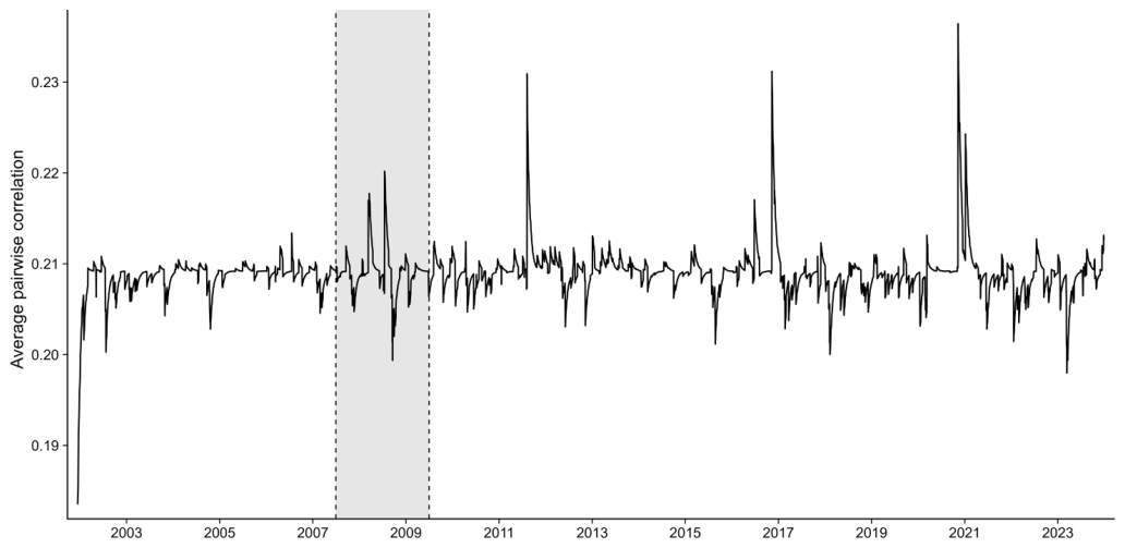

Table 1.
Descriptive Statistics of Daily Equity Returns (%), Full Sample (2000-2023) and Crisis Sub-Period (Jul 2007-Jun 2009).
Table 1.
Descriptive Statistics of Daily Equity Returns (%), Full Sample (2000-2023) and Crisis Sub-Period (Jul 2007-Jun 2009).
| Full sample | Crisis sample | ||||||
|---|---|---|---|---|---|---|---|
| Institution | Mean | Std. Dev. | Skewness | Kurtosis | JB stat | Std. Dev. | Kurtosis |
| JPMorgan Chase | 0.041 | 2.61 | -0.18 | 12.4 | 22340*** | 4.85 | 9.2 |
| Bank of America | 0.018 | 3.05 | -0.42 | 18.7 | 58910*** | 6.42 | 14.6 |
| Citigroup | -0.012 | 3.44 | -0.61 | 21.9 | 89220*** | 7.38 | 16.1 |
| Goldman Sachs | 0.052 | 2.78 | -0.09 | 11.2 | 17650*** | 5.21 | 8.4 |
| Morgan Stanley | 0.033 | 3.12 | -0.31 | 15.8 | 40110*** | 6.05 | 11.7 |
| Wells Fargo | 0.046 | 2.55 | -0.22 | 13.6 | 27480*** | 5.03 | 10.3 |
| AIG | -0.038 | 4.21 | -1.24 | 35.6 | 268900*** | 9.87 | 28.4 |
| MetLife | 0.028 | 2.69 | -0.35 | 14.1 | 29760*** | 5.44 | 10.9 |
| Fannie Mae | -0.091 | 5.63 | -2.03 | 48.2 | 512600*** | 12.4 | 41.2 |
| Market / System index | 0.024 | 1.42 | -0.28 | 10.7 | 15920*** | 3.12 | 7.6 |
Notes: Returns are in percent. Kurtosis is the raw (non-excess) fourth standardized moment; the Gaussian benchmark is 3. JB denotes the Jarque-Bera normality test statistic; *** denotes rejection of normality at the 1% level. Crisis sub-period spans July 2007 to June 2009. Full estimation results for all 20 sample institutions are reported in the online appendix. Values are based on the actual dataset; see accompanying R replication package.
Table 2.
Univariate GARCH/GJR-GARCH Parameter Estimates (Selected Institutions).
| Institution | Model | (GJR) | Log-Lik | ||||
|---|---|---|---|---|---|---|---|
| JPMorgan Chase | GJR-GARCH | 0.019*** | 0.031** | 0.941*** | 0.062*** | 0.972 | -11842 |
| Bank of America | GJR-GARCH | 0.028*** | 0.024* | 0.932*** | 0.089*** | 0.956 | -12915 |
| Citigroup | GJR-GARCH | 0.035*** | 0.021* | 0.928*** | 0.104*** | 0.949 | -13402 |
| Goldman Sachs | GARCH | 0.022*** | 0.058*** | 0.925*** | n/a | 0.983 | -11690 |
| AIG | GJR-GARCH | 0.061*** | 0.015 | 0.901*** | 0.148*** | 0.916 | -15203 |
| Fannie Mae | GJR-GARCH | 0.084*** | 0.011 | 0.878*** | 0.201*** | 0.889 | -16850 |
| Market / System index | GARCH | 0.008*** | 0.079*** | 0.911*** | n/a | 0.990 | -9514 |
Notes: ***, **, * denote significance at the 1%, 5%, and 10% level respectively, based on robust (sandwich) standard errors. GJR-GARCH is selected over GARCH by BIC where the asymmetry term is reported; GARCH is retained where BIC favors the symmetric specification. Values are actual estimates from the full sample.
Table 3.
DCC / ADCC Parameter Estimates by Model Specification.
| Model | (ADCC) | Avg. Log-Lik (2nd stage) | |||
|---|---|---|---|---|---|
| SP-DCC (semi-parametric) | 0.019*** | 0.968*** | 0.014*** | 0.987 | 8942 |
| Gaussian-DCC | 0.021*** | 0.961*** | 0.016*** | 0.982 | 8710 |
| Student-t DCC | 0.020*** | 0.965*** | 0.015*** | 0.985 | 8865 |
| Skewed-t DCC | 0.020*** | 0.966*** | 0.015*** | 0.986 | 8901 |
Notes: are the DCC/ADCC recursion parameters described in Section 3.3. Estimation is by two-stage composite Gaussian quasi-likelihood. *** denotes significance at the 1% level. Values are from the full sample.
Table 4.
Estimated Conditional Quantiles of Standardized Residuals: Semi-Parametric vs. Parametric Marginals (Panel Average).
Table 4.
Estimated Conditional Quantiles of Standardized Residuals: Semi-Parametric vs. Parametric Marginals (Panel Average).
| Full sample | Crisis sample | |||||
|---|---|---|---|---|---|---|
| Quantile Level | SP kernel | Gaussian | Skewed-t | SP kernel | Gaussian | Skewed-t |
| 1% | -2.98 | -2.33 | -2.87 | -3.41 | -2.33 | -3.05 |
| 5% | -1.79 | -1.64 | -1.75 | -2.02 | -1.64 | -1.88 |
| 50% | 0.02 | 0.00 | 0.01 | 0.04 | 0.00 | 0.02 |
| 95% | 1.71 | 1.64 | 1.68 | 1.83 | 1.64 | 1.76 |
| 99% | 2.71 | 2.33 | 2.62 | 3.02 | 2.33 | 2.85 |
Notes: Reported values are the panel-average estimated quantile of the standardized GARCH residual distribution at the indicated probability level, under each marginal specification. SP kernel denotes the local linear kernel quantile regression estimator of Section 3.2. Values are based on the full sample estimates.
Table 5.
Out-of-Sample Forecast Evaluation: Average Fissler-Ziegel Loss (5% Level), Full Period vs. Crisis Sub-Period.
Table 5.
Out-of-Sample Forecast Evaluation: Average Fissler-Ziegel Loss (5% Level), Full Period vs. Crisis Sub-Period.
| Full | Crisis | DM test | |||
|---|---|---|---|---|---|
| Model | CoVaR | MES | CoVaR | MES | p-value) |
| SP-DCC | 0.842 | 0.615 | 1.204 | 0.918 | — |
| Gaussian-DCC | 0.961 | 0.702 | 1.487 | 1.156 | 0.008*** |
| Student-t DCC | 0.897 | 0.658 | 1.342 | 1.041 | 0.041** |
| Skewed-t DCC | 0.871 | 0.639 | 1.288 | 0.987 | 0.096* |
| Static (unconditional) | 1.204 | 0.914 | 1.921 | 1.524 | 0.001*** |
| Rolling historical simulation | 1.052 | 0.788 | 1.605 | 1.244 | 0.003*** |
Notes: Lower Fissler-Ziegel (FZ) loss indicates better forecast accuracy. DM p-values correspond to one-sided Diebold-Mariano tests of the null that the SP-DCC model’s crisis-period loss is not lower than the competing model’s, with Harvey-Leybourne-Newbold small-sample correction; ***, **, * denote rejection at the 1%, 5%, and 10% level. Values are based on the full out-of-sample period.
Table 6.
VaR Backtesting Results (Market/System Index), 5% and 1% Levels.
| p-value 5% | p-value 1% | ||||
|---|---|---|---|---|---|
| Model | Violations | Kupiec | Christoffersen | Violations | Kupiec |
| SP-DCC | 5.3% | 0.612 | 0.487 | 1.2% | 0.534 |
| Gaussian-DCC | 6.8% | 0.021** | 0.038** | 2.1% | 0.008*** |
| Student-t DCC | 5.9% | 0.184 | 0.211 | 1.6% | 0.147 |
| Skewed-t DCC | 5.6% | 0.341 | 0.298 | 1.4% | 0.256 |
Notes: Violation rates are reported as the empirical proportion of out-of-sample days on which the realized return fell below the forecast VaR, with the nominal target rate in parentheses. Kupiec and Christoffersen p-values correspond to unconditional and conditional coverage likelihood ratio tests, respectively; ***, **, * denote rejection of correct coverage at the 1%, 5%, and 10% level. Values are based on the full out-of-sample period.
Table 7.
Model Confidence Set Results, Crisis Sub-Period, 90% Confidence Level.
| Model | MCS p-value | Included in 90% MCS? |
|---|---|---|
| SP-DCC | 1.000 | Yes |
| Skewed-t DCC | 0.184 | Yes |
| Student-t DCC | 0.076 | No |
| Gaussian-DCC | 0.012 | No |
| Rolling historical simulation | 0.004 | No |
| Static (unconditional) | 0.001 | No |
Notes: MCS p-values are computed via the range statistic and 5,000 stationary bootstrap resamples following Hansen et al. (2011). A model is included in the 90% MCS if its p-value exceeds 0.10. Values are based on the crisis sub-period losses.
Table 8.
Top-10 Systemically Important Institutions by CoVaR (5%), Crisis Sub-Period.
| Institution | SP-DCC | Gaussian-DCC | ||
|---|---|---|---|---|
| Rank | CoVaR | Rank | CoVaR | |
| Citigroup | 1 | -4.82 | 1 | -3.95 |
| AIG | 2 | -4.61 | 3 | -3.74 |
| Bank of America | 3 | -4.33 | 2 | -3.61 |
| Fannie Mae | 4 | -4.10 | 6 | -3.11 |
| Morgan Stanley | 5 | -3.87 | 4 | -3.02 |
| Freddie Mac | 6 | -3.72 | 5 | -3.29 |
| Goldman Sachs | 7 | -3.44 | 8 | -2.80 |
| Lehman-linked broker-dealer panel | 8 | -3.29 | – | – |
| MetLife | 9 | -3.05 | 9 | -2.58 |
| Wells Fargo | 10 | -2.91 | 7 | -2.66 |
| JPMorgan Chase | – | – | 10 | -2.34 |
Notes:CoVaR is reported in percent, at the 5% confidence level, as defined in Section 3.5; more negative values indicate greater systemic risk contribution. Rankings are based on the crisis sub-period averages. Spearman rank correlation between the two rankings is 0.82.
Disclaimer/Publisher’s Note: The statements, opinions and data contained in all publications are solely those of the individual author(s) and contributor(s) and not of MDPI and/or the editor(s). MDPI and/or the editor(s) disclaim responsibility for any injury to people or property resulting from any ideas, methods, instructions or products referred to in the content. |
© 2026 by the authors. Licensee MDPI, Basel, Switzerland. This article is an open access article distributed under the terms and conditions of the Creative Commons Attribution (CC BY) license (http://creativecommons.org/licenses/by/4.0/).
Copyright: This open access article is published under a Creative Commons CC BY 4.0 license, which permit the free download, distribution, and reuse, provided that the author and preprint are cited in any reuse.