
Submitted:
02 October 2026
Posted:
07 October 2026
You are already at the latest version
Abstract
Classical cattle-cycle theory was developed mainly in temperate, capital-intensive livestock systems, leaving its external validity under tropical, extensive production conditions less well established. Using 851 monthly slaughter observations from Colombia (1954–2024), this study integrates seasonal ARIMA and spectral methods, Bai-Perron break tests, a five-variable VAR, external-shock ARIMAX tests, and a census-anchored Kalman reconstruction of herd inventory. The Christiano-Fitzgerald component yields an average complete-cycle duration of approximately 6.1 years, while multitaper evidence is multimodal, with concentrations around 4.4–5.0 and 7.1–7.8 years. Under the reference Bai-Perron specification, BIC selects seven breaks defining eight regimes; the first four dates are stable across nearby specifications, whereas later dates are more sensitive. Slaughter's own component explains 63.6–65.2% of its 24-month forecast-error variance across alternative Cholesky orderings. Conventional VAR Granger results do not survive Toda-Yamamoto robustness tests, and climate, interest rates, and the real exchange rate add no robust predictive content. The reconstructed herd shows a marked 2011–2019 contraction followed by recovery through 2024, although its magnitude is calibration-sensitive. The results extend evidence on retention-liquidation dynamics to a tropical, extensive, dual-purpose system while showing that individual channels remain context-dependent.
Keywords:
cattle cycle
; livestock economics
; biological capital
; structural change
; state-space models
; tropical livestock systems
1. Introduction
The cattle cycle — the regular oscillation of bovine inventory and slaughter over multi-year periods — is one of the most extensively documented phenomena in agricultural economics: when prices rise, producers retain breeding females, contracting supply; when prices fall, they liquidate cows to sustain cash flow, depressing prices further and restarting the cycle [1,2]. In Colombia, this mechanism operates on one of Latin America’s largest cattle herds — approximately 29.5 million head — whose livestock sector contributes 1.4 per cent of national GDP and 20 per cent of agricultural GDP [3,4], and sustains more than one million rural jobs. Understanding its cycle is a precondition for sectoral policy compatible with bovine reproductive biology.
Previous evidence reports 10–12-year cycles for temperate systems — including the United States, Argentina, and Uruguay [5], and similarly Canada [6] — while shorter 1.3–6.4-year cycles are reported for Brazil, Chile, and Uruguay [7]. For Australia, Griffith and Alford [8] document its synchronisation with the US cycle via international prices. Existing Colombian studies are confined to periods before 2000 [9] or lack the econometric tools to jointly assess cyclical dynamics, structural change and external shocks [10]. This gap matters for the Latin American cattle-cycle literature and for economies that trade in Colombian beef.
This article addresses that gap using one of the longest monthly cattle slaughter series available for Colombia: 851 observations between January 1954 and November 2024, extending previous samples by more than two decades. For 2008–2024, monthly bovine inventory is reconstructed via a Kalman filter anchored to five census points from ICA and FEDEGAN.
The broader empirical question is therefore not only whether Colombia exhibits a cattle cycle, but how far the classical retention-liquidation mechanism travels beyond the temperate, capital-intensive settings in which it was developed. Colombia provides a demanding test because biological lags, dual-purpose production, financing conditions, market integration, and census infrastructure differ substantially from those settings.
This article makes three contributions, consistent with the retention-liquidation mechanism of Rosen, Murphy and Scheinkman [11]. First, under the reference Bai-Perron specification with a minimum regime length of approximately 10% of the sample, BIC selects seven structural breaks defining eight regimes; the first four dates are stable across nearby specifications, whereas the post-1990 dates are more sensitive to imputation and minimum regime length. Second, it reconstructs monthly national herd inventory via a Kalman-filter state-space model: the central calibration implies a peak-to-trough contraction of approximately 9.7 million head, while 54 plausible calibrations produce contractions of 7.9–11.7 million head and substantially wider conditional state uncertainty during the 2014–2019 census gap. Third, it offers a systematic test of the three external shocks most commonly invoked in the cattle-cycle literature — climate, monetary policy, and the real exchange rate — finding no robust incremental predictive content from any, a result that contrasts with credit-channel effects documented for temperate, capital-intensive systems.
2. Theoretical Framework
2.1. Endogenous Dynamics, Expectations, and Biological Capital
The characterisation of the cattle cycle has moved from descriptive empirical observations [12,13] toward formulations that integrate the intertemporal dynamics of biological capital. The contemporary consolidation of the field came with the rational-expectations framework of Rosen, Murphy and Scheinkman [11]—RMS— in which the producer maximises the present value of future cash flows subject to reproductive constraints. Under this approach, the oscillations do not reflect irrationality but rather the equilibrium trajectory of a dynamic system governed by difference equations with complex conjugate roots, whose imaginary part defines the cycle’s angular frequency [5].
The mechanical core of the cycle lies at the intersection of reproductive biology and herd financial management. Supply available in period t is a function of female-retention decisions made k periods earlier —where k incorporates gestation, lactation and rearing [14]—, turning the herd into a heterogeneous capital stock whose age distribution determines the future path of supply. Heterogeneous expectations — rational and naive agents coexisting — amplify the aggregate oscillation [15,16]. Whether Colombia’s lower average financial capacity to sustain cow retention through prolonged low-price phases compresses cycle periodicity relative to mature markets — where strategic retention sustained by greater credit access lengthens the cycle — is a plausible hypothesis rather than an established finding for the Colombian case; Section 5.6 evaluates it directly and finds no significant effect from the policy interest rate, though the quantity-rationing channel distinct from price remains untested [17,18].
Although the cycle is endogenous in origin, its observed trajectory is distorted by exogenous shocks. Climatic events alter forage availability and induce early liquidation that transiently accelerates contractionary phases [6,19]. At the macroeconomic level, credit constraints operate as a financial accelerator: during monetary tightening, producers face negative cash flows that force premature cow sales [20]. In Colombia, it has been suggested that the consolidation of the dual-purpose system diversified producers’ cash flows1, potentially easing liquidity constraints during low-price phases and dampening the financial accelerator [21,22]; this remains a plausible but empirically untested mechanism for the Colombian case (Section 5.6). Empirically identifying these transitions requires the Bai and Perron [23] algorithm, complemented by CUSUM/MOSUM tests [24].
The RMS mechanism therefore provides a common theoretical benchmark, while cycle duration, amplitude, and apparent sensitivity to shocks may vary with biological parameters, financing constraints, market integration, and productive structure. This distinction between a portable mechanism and context-dependent empirical manifestations motivates the Colombian test developed below.
2.2. The Cattle Cycle in Colombia: Context and Literature
For Colombia, pioneering studies by the Centro de Estudios Ganaderos y Agrícolas (CEGA) and FEDEGAN identified five complete cycles between 1950 and 1978, averaging 6–7 years in length [25]—shorter than the 8–12-year range found in the North American literature [11], a difference plausibly related to Colombia’s biological parameters and production conditions rather than attributable to any single confirmed cause (Section 5.6). Lorente [2,9] extended the herd’s demographic analysis and quantified the reduction in slaughter age from 57 to 35 months between 1958 and 1993 —a technological advance that shortened the cycle’s biological lag. García [26] estimated, for 1945–1975, a contemporaneous slaughter price elasticity of −0.64 and a three-year elasticity of +0.69, confirming cobweb-type behaviour. He also documented that trade policy rendered the Colombian cattle sector effectively non-tradeable, unlike exporting economies such as Canada [6] or Australia [8]. Compounding these are institutional disturbances with no international parallel —violence, forced displacement, extreme land concentration with a Gini coefficient of 0.91 [27] — which introduce breaks in the slaughter trend without altering the cycle’s underlying periodicity.
2.3. Formal Model
Following Rosen, Murphy and Scheinkman [11] and the notation of Mundlak and Huang [5], adapted for Colombia by Lorente and Vargas [9], the model employs the parameters in Table 1.
The fundamental biological constraint is the population-accounting equation of order ab:
The left-hand side sums female slaughter sf(t) and the stock of breeding cows F(t) at t. The right-hand side states that this total derives from the surviving stock of the previous period plus the females that have just reached breeding age. The intertemporal arbitrage condition establishes that a producer retains a female whenever the present value of her future calves exceeds the immediate net return from slaughter:
where qt = pt − mt is the net return on sale and β = 1/(1 + r) is the discount factor. Combining the biological constraint (1), the arbitrage condition (2), and demand ct = α₀−αpt + dt, the system reduces to:
where L is the lag operator and Ωt collects the exogenous shocks. The complex conjugate roots of the characteristic equations generate the oscillatory behaviour: a positive demand shock raises pt, induces female retention, expands F(t) in subsequent periods, and the resulting future excess supply depresses prices, restarting the cycle. Cycle duration is determined by the modulus r and the angle θ of the complex roots φj = r ⋅ e±iθ, with approximate period T = 2π/θ [9]. Since θ depends on ab and g, any technological change that lowers the age at entry into breeding or raises fertility alters the cycle’s periodicity.
(1 − φ1L)(1 − φ2L)(1 − φ3L)xt = Ωt
(1 − λ1L)ct = −(1 − φ1L)Ωt
2.4. Inventory as a State Variable
The RMS model treats bovine inventory Xt as a latent state variable whose trajectory determines the future supply of meat. Monthly slaughter is a “noisy”2 realisation of extraction decisions, not a direct measure of the herd. Equation (1) implies that Xt+1 = (1 + g)Xt − St, an expression formally equivalent to the state equation of a linear state-space model [28], which makes the Kalman filter the optimal estimator of the herd under normality: it recursively updates the estimate of Xt by weighting the biological model’s prediction against the information available from census inventories, whose irregular multi-year frequency leaves only sparse observations of the measurement equation Yt = Xt + εt.
The central parameter of the state model, g, is often conflated with the gross birth rate —the ratio of births to breeding-age females, which in Colombia runs at roughly 43–50 per cent annually [29]— and the net growth rate of the total herd, which nets out natural mortality and incorporates the inventory’s age and sex structure. The equilibrium condition implies g* = S̅ / X̅, where S̅ and X̅ are mean slaughter and the reference inventory, respectively [15].
The Kalman gain Kt = Pt|t−1 / (Pt|t−1 + R) has a direct economic interpretation: it weights the credibility of the state prediction against the census observation, with values near 1 giving greater weight to the census update. The implicit extraction rate et = St / Xt links inventory to the cycle: in the theory of Jarvis [1] and Rosen [53], et falls during cow retention and rises during liquidation. A countercyclical extraction rate is therefore a pattern consistent with the retention-liquidation mechanism, while the Kalman reconstruction supplies an estimate of the otherwise sparsely observed herd stock.
3. Materials and Methods
3.1. Data
The central variable is monthly bovine slaughter in Colombia, disaggregated by sex. The series, from DANE’s Cattle Slaughter Survey (ESAG), covers January 1954–November 2024 (851 observations) — the longest such series analysed for the country, extending previous studies’ samples by more than two decades [9,10]. Fifty of the 851 monthly observations (5.9 per cent) are missing, concentrated in two multi-month gaps (1969–1970 and 1999–2000, the latter coinciding with a documented DANE-ESAG methodology change) rather than randomly distributed. The primary series is completed with an STL-aware interpolation that uses the seasonal structure of the monthly series; simple linear interpolation is retained as a sensitivity specification. Under the reference Bai-Perron trimming, both methods select seven breaks, but the post-1990 break dates are materially more sensitive to the imputation choice than the first four dates (Section 4.4).
The multivariate analysis of price mechanisms uses five monthly series for January 1990–February 2000 (122 obs., detailed in Table 2). For macroeconomic shocks, the Banco de la República’s interest rate and the ITCR-IPC-NT are incorporated for April 1995–November 2024 (356 obs.); a Chow test confirms a highly significant structural break in this series in October 1999 (F = 1606.1, p < 0.001), coinciding with Colombia’s move from the exchange-rate band regime to inflation targeting, with additional breaks in 2009 and 2021 consistent with the global financial crisis and post-pandemic tightening (Section 5.7). The climate cycle is proxied by an ordinal ENSO index for 1954–2024, coded from −3 (strong El Niño) to +1 (La Niña), with 0 denoting neutral conditions. Slaughter and the strictly positive price/quantity series are natural-log transformed. ENSO, the policy rate, and the ITCR are retained in their native scales. Where the external-shock protocol uses first differences, slaughter enters as Δlog(slaughter) and the external variables are differenced in their native scales; ARIMAX regressors enter in levels according to each specification.
Monthly bovine inventory for the October 2008–December 2024 subperiod is estimated via a Kalman-filter state-space model [28]. The state equation is:
where g is the monthly equilibrium replacement-flow parameter, calibrated at 1.147 per cent as the ratio of mean monthly total outflow (slaughter plus live exports) to the 2008 reference inventory of 27.0 million head — St is monthly total outflow (slaughter plus live exports), and ηt∼N(0,Q) is the process disturbance. The measurement equation:
links the latent state Xt to five ICA and FEDEGAN census anchors (2008, 2010, 2014, 2019 and 2022), with εt∼N(0,R) as measurement error. The Kalman gains at the four update points following the initial 2008 anchor (used to set the model’s starting state and variance) ranged between 0.93 and 0.97, giving predominance to census observations over the model prediction. The central calibration sets Q = (300,000)2 as the process-noise variance, R = (600,000)2 as the census-measurement variance, X0 = 27,000,000 head, and P0 = (1,500,000)2. Parameter sensitivity is evaluated over 54 specifications combining g at ±10% of its central value, process-noise standard deviations of 200,000, 300,000, and 400,000 head, measurement-error standard deviations of 500,000, 600,000, and 800,000 head, and initial-state standard deviations of 1.5 and 2.0 million head. The flow data come from FEDEGAN’s monthly series (195 observations), disaggregated by sex and including live exports.
Xt+1 = (1 + g)Xt − St + ηt
Yt = Xt + εt
3.2. Empirical Strategy
Characterising the long-run dynamics of a livestock system requires more than fitting a single model to a single series: the retention-liquidation mechanism linking a biological process (herd reproduction), an economic decision (retain or liquidate breeding stock), and a partially observed state variable (the herd, measured only through periodic censuses) is addressed by no single econometric technique. This section applies an integrated framework in which each method answers one of four sequential questions: does a cycle exist and at what periodicity; has the growth process undergone structural change; how do prices and quantities interact dynamically, including external shocks; and what does this imply for the unobserved stock of breeding capital estimated in Section 3.1?
The biological reproduction lag in cattle production bounds how quickly supply can respond to price; establishing whether a cycle exists, and at what periodicity, without assuming a duration a priori, is the necessary first step. Each series’ order of integration is determined via three complementary tests: augmented Dickey-Fuller [30,31], Phillips-Perron [32], and Kwiatkowski-Phillips-Schmidt-Shin [33]. STL decomposition [34] is summarised using trend and seasonal strength measures rather than variance shares, because STL components are not orthogonal. Values close to one indicate a component that is strong relative to the remainder; the STL remainder is not interpreted as the cattle-cycle component.
Cycle identification proceeds via multiple frequency- and time-domain methods rather than a single technique, following the spectral approach of Mundlak and Huang [5]. To ensure robustness, three versions of the spectrum are estimated: the raw periodogram, a smoothed spectral density using a modified Daniell window, and Thomson’s [35] multitaper estimator using four tapers with time-bandwidth parameter NW = 2.5. The analysis is applied to the first log-difference of the slaughter series, which removes the stochastic trend without imposing the seasonal-decomposition assumptions that STL requires. In addition, the Baxter-King [36] and Christiano-Fitzgerald [37] filters extract the cyclical component in the 4-to-12-year range. Spectral frequencies are expressed in cycles per year, so period in years is computed as the reciprocal of frequency; this time scale is verified against a synthetic six-year monthly cycle. Cycle duration is dated from complete peak-to-peak and trough-to-trough intervals in the Christiano-Fitzgerald component, using a 48-month minimum separation as the reference rule and 36- and 60-month separations as sensitivity checks.
The short-run autoregressive structure implied by the retention-liquidation mechanism is characterised via seasonal ARIMA modelling, following the iterative Box-Jenkins protocol [38] across 200SARIMA(p,d,q)(P,D,Q)12 specifications, selected using the corrected Akaike information criterion [39], the Bayesian information criterion (BIC), and Akaike weights. Residual diagnostics include the Ljung-Box test (autocorrelation), the ARCH-LM test [40] (conditional heteroscedasticity), and the Jarque-Bera test (normality). Box and Tiao’s [41] intervention analysis identifies historically documented outliers via pulse variables incorporated as external regressors in the ARIMA model.
Technological and institutional change may alter the level or trend of slaughter discretely rather than continuously. Parameter stability is assessed with Andrews’ [31] QLR test, the Bai and Perron [23,42] algorithm, and CUSUM/MOSUM tests [24]. The reference Bai-Perron specification uses a minimum regime length of 85 months (approximately 10% of the 851-observation sample), matching the pre-specified trimming rule in the original analysis; BIC selects the number of breaks. Robustness is assessed at minimum regime lengths of 60, 72, 96 and 120 months and under linear rather than STL-aware imputation. Because log slaughter is I(1), a mean-break specification in Δlog(slaughter) is also estimated as a robustness check; it is interpreted separately from level/trend segmentation. The retention-liquidation decision is a feedback system requiring a dynamic multivariate framework. Price mechanisms are analysed via a VAR model [43] with five endogenous variables in logarithms, Johansen cointegration tests [44], conventional Granger predictive-causality tests [45], and impulse-response functions with bootstrap confidence bands (500 replications). Inference in level VARs with unit roots can be non-standard [51]; predictive-causality inference is therefore also checked with Toda-Yamamoto augmented-lag Wald tests (p = 1, dmax = 1) [54]. Baseline orthogonalised IRFs and FEVDs use the Cholesky ordering cattle price → slaughter → poultry price → pork price → milk price; robustness is assessed under three alternative orderings. The effect of each external shock — climate, interest rate and ITCR-IPC-NT — is assessed through a unified three-step protocol: a cross-correlation function (CCF) in first differences, Granger predictive-causality in a bivariate VAR, and an ARIMAX model with a likelihood-ratio test (LRT) against the baseline model. All analysis was conducted in R 4.5.0 [46], using the forecast, strucchange, vars and multitaper packages and a custom Kalman-filter implementation. A generative AI tool (Anthropic Claude) was used during manuscript preparation for language and editorial refinement. All statistical computations were executed in R by the authors, who reviewed the code, validated the outputs against the study data, and retained responsibility for all methodological choices, results, and interpretations.
4. Results
4.1. Statistical Characterisation of the Bovine Slaughter Series
Figure 1 presents the evolution of monthly bovine slaughter in Colombia (1954–2024) alongside the proportion of females — a central indicator of the cycle’s phase [1]. Three features dominate: a positive trend that took slaughter from 103,000 head/month in 1954 to 270,000 in the 2010s; persistent cyclicality across the seventy-year span; and marked variation in cyclical amplitude over time, with particularly large oscillations in some mid-sample regimes and much lower amplitude in the two most recent regimes (Figure 4), a pattern potentially consistent with technological dampening [5]. The proportion of females — 24.0 to 53.1 per cent, averaging 39.5 per cent — traces the cycle’s phases: peaks mark forced liquidations, troughs mark retention.
STL decomposition [34] yields a trend strength of 0.921 and a seasonal strength of 0.140, indicating a very strong low-frequency trend and comparatively weak seasonality. The STL remainder is not labelled a cyclical residual; cycle dating is based instead on the spectral and band-pass procedures in Section 4.3. Expansions are generally longer than contractions, consistent with herd rebuilding taking more time than liquidation [11].
Table 3 presents the unit-root tests. The ADF, Phillips-Perron and KPSS tests converge unanimously: the series is integrated of order one, I(1), non-stationary in levels and stationary in first differences. This diagnostic determines the ARIMA specification with d = 1.
4.2. Arima Modelling with Intervention Analysis
The search across 200 SARIMA specifications by AICc identifies SARIMA(2,1,1)(1,0,1)12 as optimal (AICc = −2,804.75; Akaike weight = 1.0; Table 4), constituting substantial evidence [47]. All parameters are highly significant (Table 5). The AR(1) and AR(2) coefficients are both negative and capture statistically significant short-run serial dynamics; their implied root structure is compatible with oscillatory adjustment but should not be interpreted as direct identification of the long-run cattle-cycle periodicity in the retention-liquidation framework [11]. The near-unit SAR(1) = 0.996 reflects strong seasonal persistence, corrected by SMA(1) = −0.916.
Intervention analysis [41] identifies five statistically significant pulse interventions (Table 5; Figure 2): Dec. 1966, Dec. 1968, Jan. 2009, Apr. 2020, and May 2021. These dates coincide with historically salient episodes, but the intervention dummies identify statistical outliers rather than their causes; in particular, the Jan. 2009 pulse is not interpreted as an ENSO-caused liquidation given the external-shock results in Section 4.6. Including the pulses reduces residual kurtosis from 10.47 to 4.58; the ARCH test detects no heteroscedasticity (p = 0.570).
4.3. Spectral Analysis and Cycle-Extraction Filters
Spectral analysis of the first log-difference of the slaughter series reveals the cattle cycle’s frequency signature, avoiding the seasonal-harmonic leakage that an STL residual would introduce. Thomson’s [35] multitaper estimator is multimodal, with prominent concentrations around 4.38–5.02 years and 7.11–7.76 years rather than a single dominant frequency. The smoothed Daniell spectrum also concentrates substantial power around roughly 6–8 years. These estimates are therefore interpreted as a broad multi-frequency cycle rather than evidence for one invariant periodicity.
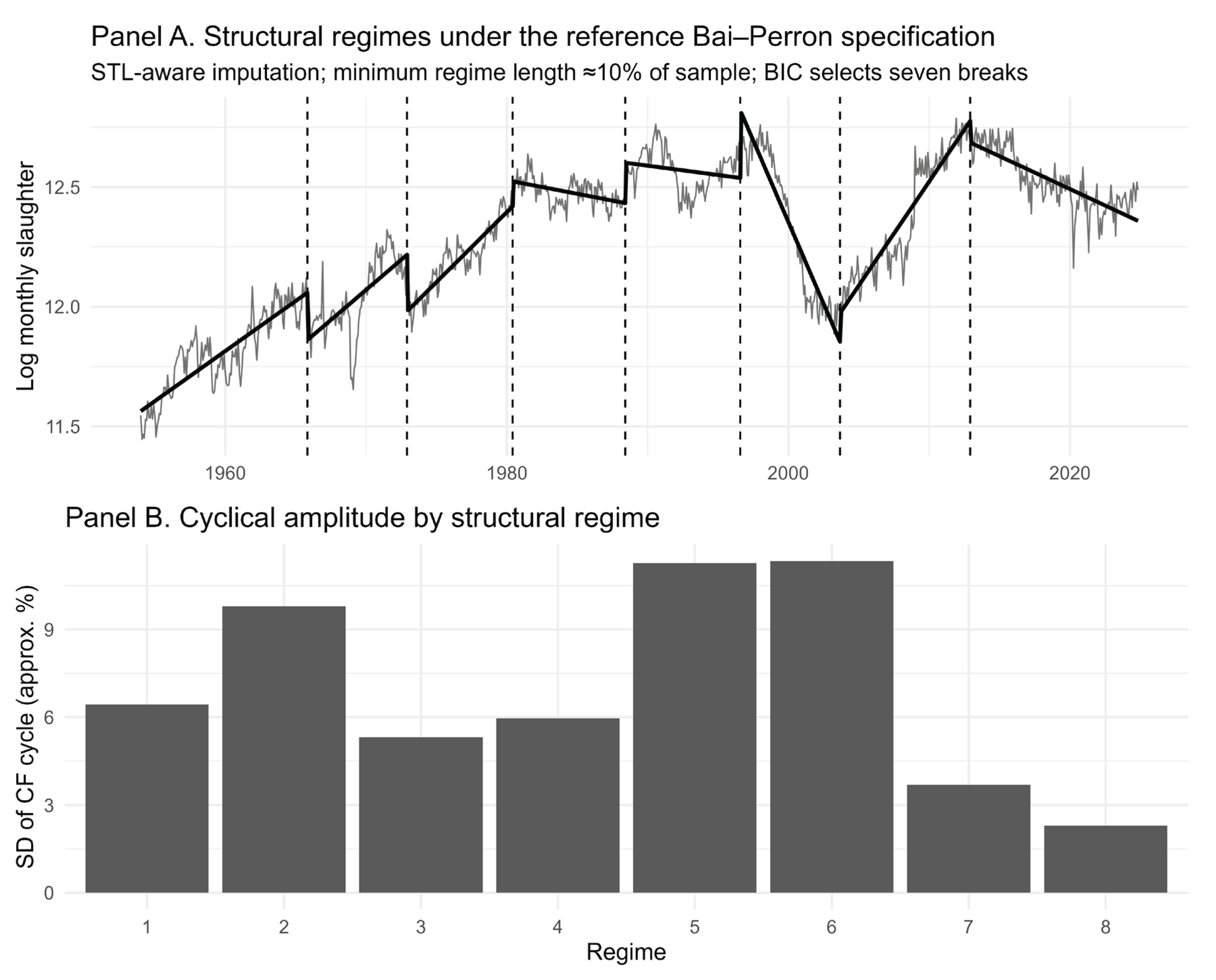
The Christiano-Fitzgerald filter (48–144 months) provides a reproducible turning-point chronology (Figure 3). Using a 48-month minimum separation, 11 complete peak-to-peak intervals average 6.11 years and 11 trough-to-trough intervals average 6.15 years; the combined summary is approximately 6.13 years. Complete-cycle durations range from about 4 to 10 years. The approximately 6.1-year result is therefore based on dated CF turning points rather than on a single spectral peak or on structural-regime lengths. Figure 4 reports cyclical amplitude by the eight regimes of the reference break specification.
4.4. Structural Change in Bovine Slaughter Dynamics
Andrews’ [31] QLR test rejects the hypothesis of parametric stability (supF = 1,144.4; p < 0.001). The Bai and Perron [23,42] algorithm selects seven breaks under the reference minimum regime length of 85 months (approximately 10% of the sample), with the BIC optimum lying inside the admissible search range rather than at its boundary (Table 6). The selected count is sensitive to the minimum regime length: BIC selects 11, 8, 7, 7, and 5 breaks for h = 60, 72, 85, 96, and 120 months, respectively; at h = 96 the seven-break solution lies at the admissible boundary. The first four reference dates are highly stable across nearby STL/linear specifications (maximum shifts of 0–2 months), whereas the 1996, 2003, and 2012 dates shift by as much as 37–48 months. Conditional confidence intervals in Table 6 therefore describe dating precision within the reference model and should not be confused with cross-specification stability (Figure 4).
The first two breaks (November 1965 and December 1972) coincide with major transformations in the Colombian cattle sector [18]: the reduction in slaughter age from 57 to ~35 months [2,9] and the progressive elimination of the rearing period, historically associated with the introduction of improved pastures and INCORA’s intervention [25]. The profitability of beef exports grew sharply between 1968 and 1972, reaching its historical peak that year, as documented in [26].
Figure 4.
Structural regimes of Colombian bovine slaughter, 1954–2024. Note: Top panel: log(slaughter) and segmented trends under the reference Bai-Perron specification (STL-aware imputation; h = 85 months). Vertical dashed lines mark the seven reference break dates. Bottom panel: cyclical amplitude, measured as the standard deviation of the Christiano-Fitzgerald cycle within each reference regime (approximately percentage units). See Table 6 and the text for conditional dating intervals and cross-specification sensitivity. Source: DANE-ESAG. Authors’ calculations.
Figure 4.
Structural regimes of Colombian bovine slaughter, 1954–2024. Note: Top panel: log(slaughter) and segmented trends under the reference Bai-Perron specification (STL-aware imputation; h = 85 months). Vertical dashed lines mark the seven reference break dates. Bottom panel: cyclical amplitude, measured as the standard deviation of the Christiano-Fitzgerald cycle within each reference regime (approximately percentage units). See Table 6 and the text for conditional dating intervals and cross-specification sensitivity. Source: DANE-ESAG. Authors’ calculations.
The June 1980 break coincides with the close of the fourth cattle cycle independently dated by Lorente [2] using CEGA data (1976–1981), marking a pronounced slowdown. FEDEGAN [48] and Kalmanovitz and López [20] document that closing external markets and falling real prices from 1978 contracted slaughter incentives. García [26] provides the full chronology. The following break, in June 1988, falls within the transition documented by Jaramillo and Caicedo [21] around 1990 toward the dual-purpose system, suggested but not directly tested as a mechanism for declining cyclical amplitude (Section 5.6).
In the reference STL-aware specification, breaks 5 and 6 bound an extended contraction regime from August 1996 to September 2003. Unlike the first four breaks, however, these later dates are specification-sensitive: with linear interpolation and the same h = 85 months, the corresponding late break sequence shifts to August 2000 and December 2008; with h = 72 months, the reference sequence places later breaks around 1996, 2002, 2008, and 2016. The reference contraction overlaps the 1999 recession and the documented DANE-ESAG discontinuity. FEDEGAN [48] documents that the proportion of females slaughtered reached 42.2 per cent in 1998 — the series’ historical maximum. Because the largest missing-data gap lies in this interval, interpretation should attach to the broad shift rather than to an exact month. In the reference specification, the regime following September 2003 expands through December 2012. The ESAG methodological redesign, the closure of municipal abattoirs [49], the 2009–2016 adverse-climate cycle [19], and the global financial crisis fall within a period in which exact break placement is sensitive; they are therefore treated as historical context rather than assigned as causes of a uniquely dated break.
The seventh reference break occurs in December 2012, close to the onset of the 2011–2019 contraction in the census-anchored stock-flow reconstruction (Section 4.7). This coincidence should not be described as independent confirmation: the state equation uses observed slaughter and exports between census anchors, although its census observations come from a separate source. Moreover, the late break date is specification-sensitive; with linear interpolation at the same h = 85 months, the corresponding final break is January 2016. The inventory reconstruction therefore corroborates the broad contraction-recovery phase, not a uniquely identified December 2012 structural date.
Figure 4 shows strongly heterogeneous cyclical amplitude rather than a monotonic secular decline: amplitude is highest in reference regimes 5 and 6 and falls sharply in regimes 7 and 8. The recent dampening is qualitatively consistent with evidence reported by Li and Shonkwiler [50] for the United States and by Twine et al. [6] for Canada, but Colombia’s full-sample amplitude path is non-monotonic. Candidate contributing mechanisms for the lower recent amplitude are discussed in Section 5.6.
4.5. Multivariate Analysis: Price Mechanisms
The VAR(1) estimated for January 1990–February 2000 operates over five endogenous variables in logarithms (Table 2). The Johansen trace test rejects the null of no cointegration (r = 0) at the 1 per cent level only marginally (trace = 84.60; 1% critical value = 84.45), while the null r ≤ 1 is not rejected even at 10 per cent (45.83 < 49.65). The maximum-eigenvalue test also rejects r = 0 at 5 per cent (38.77 > 34.40), but not at 1 per cent (39.79), and does not reject r ≤ 1. Taken together, the tests support one cointegrating relation rather than an absence of cointegration. The BIC selects a stable VAR(1) — maximum root 0.982 — with no conditional heteroscedasticity (multivariate ARCH: p = 0.103). Because standard causality tests can be sensitive to the integration/cointegration specification, Toda-Yamamoto inference is reported as a robustness check [54].
The conventional VAR(1) Granger tests in Table 7 indicate bidirectional price-slaughter predictability and significant baseline associations from milk and poultry prices to slaughter. These findings are not robust to Toda-Yamamoto inference: the augmented-lag Wald tests do not reject non-causality for cattle price → slaughter (p = 0.177), slaughter → cattle price (p = 0.537), milk price → slaughter (p = 0.214), poultry price → slaughter (p = 0.150), or pork price → slaughter (p = 0.136). The VAR(1) results are therefore treated as specification-dependent predictive associations consistent with the proposed mechanism, rather than as robust evidence of causal direction.
Figure 5 presents the baseline orthogonalised impulse-response function of cattle price to a shock in slaughter with 95 per cent bootstrap confidence bands (500 replications). Under the baseline ordering, the point estimate is negative in the initial months and turns positive around month 9. Across the four Cholesky orderings examined, the negative-to-positive crossing occurs between months 9 and 12 and the response amplitude changes, indicating some ordering sensitivity. Moreover, the 95 per cent bootstrap confidence bands for the baseline IRF include zero at every horizon tested (0–24 months). The lag should therefore be read as suggestive rather than precisely identified. As reported in Table 8, the FEVD result is more stable to ordering: own shocks account for 63.6–65.2 per cent of the 24-month slaughter variance, while cattle price remains the largest external contributor at 14.6–15.9 per cent.
4.6. External Shocks: Climate, Interest Rates, and the Real Exchange Rate
This section tests whether climate, interest rates, and the real exchange rate anticipate slaughter or improve the ARIMA model’s predictive capacity, using the same protocol for all three: a cross-correlation function (CCF) in differences, Granger predictive-causality in a bivariate VAR, and ARIMAX with an LRT against the baseline SARIMA (Figure 6). None of the three provides robust incremental predictive content.
Climate. The ENSO index shows no robust association with slaughter under any of the three tests (Table 9). This does not contradict the descriptive evidence: months coded as strong El Niño are associated with average slaughter 7.86 per cent above neutral months and a female-slaughter proportion of 0.410. These descriptive differences are episodic associations rather than identified causal effects. Under the Monte Carlo design used for the post-hoc power exercise, the climate test reaches 80 per cent power for standardised effects of approximately 0.015; relative to the interest-rate test, it is therefore comparatively sensitive, while remaining conditional on the simulation design (Section 5.7).
Interest rate. The CCF, Granger, and ARIMAX tests find no significant association with slaughter (Table 9). This result is consistent with García’s [26] finding that subsidised credit did not raise Colombian cattle-sector profitability. The power analysis indicates this test is markedly less sensitive than the climate or exchange-rate tests (minimum detectable effect ≈ 0.095 standardised units); a moderate true effect cannot be fully excluded (Section 5.7).
Real exchange rate. The CCF, Granger, and ARIMAX tests find no robust association running from the ITCR-IPC-NT to slaughter (Table 9). Reverse-direction predictive tests show nominal p-values below 0.05 at some lags, but none survives the Bonferroni correction for the four tests performed. The power analysis indicates this test is sensitive to standardised effects as small as 0.032. This is consistent with García [26]’s documentation of Colombia’s historically non-tradeable cattle sector (Section 2.2).
Taken together, Table 9 and Figure 6 indicate that, under the proxies and specifications tested here, climate, the policy rate, and the real exchange rate provide no robust incremental predictive content for monthly Colombian bovine slaughter beyond its own dynamics; the interest-rate result should be read with the power caveat above.
4.7. Bovine Herd Inventory: Monthly Estimation via Kalman Filter
To bridge the multi-year gap between agricultural censuses, the Kalman-filter state-space model described in Section 3.1 was implemented. Under the central calibration, the Kalman gain at the four update points following the initial anchor ranged between 0.93 and 0.97, giving predominance to census observations over model prediction when an anchor is available (Figure 7). Across the 54 parameter-sensitivity specifications, realised gains remain high overall (0.839–0.989), confirming that census anchors dominate the updates under the full calibration grid.
Note: Solid line: point estimate of monthly inventory (million head). Shaded band: 95% conditional state-uncertainty band (±1.96√Pt) propagated by the Kalman filter for the fixed central calibration; it is not a confidence interval for the peak-to-trough contraction itself. Red triangles (▲): ICA/FEDEGAN census inventories used as anchors (2008, 2010, 2014, 2019, 2022). The band widens during the unanchored 2014–2019 gap. Source: FEDEGAN; ICA. Authors’ calculations.
Under the central calibration, the herd trough is 18.19 million head in May 2019, and the central peak-to-trough point estimates imply a contraction of approximately 9.7 million head. The conditional state-uncertainty band widens substantially during the long unanchored interval before the 2019 census; because the covariance of the peak-trough difference is not estimated here, marginal state bands are not interpreted as a 95% confidence interval for contraction magnitude. Parameter sensitivity points in the same direction but broadens the level estimates: across 54 calibrations, the trough ranges from 16.07 to 21.21 million head, the peak-to-trough contraction from 7.90 to 11.67 million head, and the end-2024 inventory from 29.77 to 33.53 million head. Thus the contraction-recovery pattern is robust to plausible calibration changes, while its exact magnitude is not. The proportion of females in slaughter — 45.4 per cent in 2013 — is consistent with elevated liquidation pressure during the contraction phase without crossing the 50 per cent threshold. The COVID-19 slaughter reduction in 2020 (3.26 million versus 3.41 million in 2019) is consistent with temporary retention of animals otherwise slaughtered (Table 10).
The implicit extraction rate (Figure 8) traces a countercyclical pattern relative to inventory, a pattern consistent with the RMS mechanism. Its mean value was 14.9 per cent annually (Table 10), consistent with the historical ranges reported by Cuenca, Chavarro and Díaz [29]. Rates were elevated during the 2015–2019 contraction (18–19 per cent) and declined during the subsequent expansion (to 10.4 per cent in 2023).
The proportion of females in slaughter (Figure 9) serves as a leading indicator of the cycle’s phase, peaking at 45.4 per cent in 2013 before stabilising during the expansion, consistent with selective slaughter of non-breeding animals. Its failure to cross the 50 per cent threshold indicates the sector did not reach the reproductive collapse seen in previous episodes [9]. Live exports grew steadily over the period (Table 10); their modest share (3.22 per cent of total outflow) is an additional observed outflow channel. Taken together, Table 10 and Figure 7, Figure 8 and Figure 9 present an internally consistent picture: the independently observed female-slaughter share and census anchors support the phase interpretation, while the extraction rate is itself partly derived from the estimated inventory and should not be treated as independent validation. The direction of contraction and recovery is clearer than the precise magnitude of the trough.
5. Discussion
Viewed through an external-validity lens, the Colombian evidence asks not only whether a cattle cycle exists, but which elements of the classical retention-liquidation mechanism persist when biological, financial, and institutional conditions differ sharply from those of temperate cattle economies. The discussion therefore separates features that appear to travel across settings—cyclical persistence and strong internal propagation—from features whose magnitude, timing, or interpretation remain context-dependent.
5.1. The Cycle Shows Persistence and Internal Propagation, and Is Shorter than in Developed Cattle Economies
The average complete-cycle duration of approximately 6.1 years is consistent with prior Colombian estimates, including Lorente [9] and Rojo and Escobar [10], and with the shorter range documented internationally (Section 5.6). Biological and technological parameters offer a plausible explanation for this shorter periodicity: Mundlak and Huang [5] show that cycle duration is linked to the order of the biological difference equation. With slaughter age declining to about 35 months by 1993 [2,9], the Colombian evidence is consistent with a shorter biologically constrained cycle; this interpretation is not a separately identified causal effect.
The evidence is consistent with strong internal propagation, supported most directly by two results: (i) slaughter’s own component explains 63.6–65.2 per cent of its 24-month forecast-error variance across alternative Cholesky orderings; and (ii) none of the three external variables tested — climate, interest rate, exchange rate — provides robust incremental predictive content over the baseline ARIMA model, although the power analysis (Section 5.7) is less sensitive for the interest rate. The negative AR(1) and AR(2) coefficients capture significant short-run serial dynamics but are not treated as direct identification of the long cattle-cycle periodicity. This should not be read as evidence that the sector is insulated from macroeconomic or climatic conditions in any absolute sense — only that none of the proxies tested shows robust incremental predictive content beyond the series’ own history. This interpretation is consistent with Aadland [16], who shows that heterogeneity in producers’ expectations is a sufficient condition for the cycle to emerge endogenously.
5.2. Structural Transformation Is Concentrated in Specific Episodes, Not a Single Turning Point
Under the reference Bai-Perron specification (minimum regime length ≈10% of the sample), BIC selects seven structural breaks defining eight regimes. This count is not invariant to the minimum regime length: shorter admissible regimes produce more breaks and longer admissible regimes fewer. The first four reference dates (1965, 1972, 1980, 1988) are highly stable across nearby STL/linear specifications, whereas the post-1990 dates are materially more sensitive. The consolidation of the dual-purpose system, plausibly associated with the transition around the stable 1988 break, may dampen the financial-accelerator mechanism discussed in Section 2.1 (Bierlen, Dixon and Ahrendsen [52]); this remains a plausible but empirically untested mechanism for the Colombian case (Section 5.6).
Cyclical amplitude is also non-monotonic across the eight reference regimes (Figure 4): regimes 5 and 6 show the largest CF-cycle dispersion, followed by a sharp decline in regimes 7 and 8. The low recent amplitude is consistent with a dampening interpretation, but the full historical path does not support a simple secular decline. A January 2016 break appears under some sensitivity specifications, including linear interpolation at h = 85 months, so the reference December 2012 date should not be presented as uniquely determined. The recent deceleration remains descriptively visible even when its exact break date is specification-sensitive.
5.3. Price-Slaughter Dynamics Are Consistent with the Cycle Mechanism, but Causal Evidence Is Specification-Dependent
The conventional VAR(1) Granger tests suggest bidirectional price-slaughter predictability — price → slaughter (p = 0.0004) and slaughter → price (p = 0.011) — consistent with the feedback mechanism described by Jarvis [1] and Rosen, Murphy and Scheinkman [11]. However, this inference is specification-dependent: Toda-Yamamoto tests do not reject non-causality in either direction (p = 0.177 and p = 0.537, respectively), and neither the milk, poultry, nor pork price channel is significant under the same robustness procedure (all p > 0.13). The orthogonalised IRF of price to a slaughter shock also remains imprecise: its point estimate shifts from negative to positive between months 9 and 12 across alternative Cholesky orderings, while the baseline 95 per cent bootstrap confidence bands include zero at every horizon. The multivariate evidence is therefore consistent with a price-quantity feedback mechanism but does not robustly identify either causal direction or a precise biological lag.
5.4. The Structural Breaks Coincide with Technological and Institutional Change
The seven reference breaks coincide with a sequence of technological, institutional, and historical episodes (Section 4.4), but the strength of the dating evidence differs across the sample. The first four dates (1965, 1972, 1980, 1988) move by at most 0–2 months across nearby specifications and occur alongside changes in slaughter age, pasture expansion, and cycle turning points documented by Lorente [2]. By contrast, the 1996, 2003, and 2012 reference dates shift by roughly three to four years under some alternative imputation/trimming choices. The 1999 recession, DANE-ESAG discontinuity, and the 2011–2019 herd contraction therefore provide historical context for the later segmentation but do not establish uniquely dated causal breaks. None of these temporal correspondences identifies a monetary- or exchange-rate-policy cause, consistent with the absence of robust incremental predictive content from the policy-rate and ITCR variables (Section 4.6). Export profitability rose sharply from 1962, peaked in 1972, and reversed from 1974 onward [26], temporally aligning with the acceleration of the 1972–1980 reference regime and subsequent slowdown.
5.5. Inventory Dynamics Are Consistent with the Rms Mechanism, with Substantial Uncertainty in the 2015–2019 Trough
The Kalman-filter estimation of bovine inventory adds the trajectory of the biological capital stock that slaughter alone cannot observe directly. Under the central calibration, the 2011–2019 point estimates imply a contraction of approximately 9.7 million head; across 54 calibration variants the peak-to-trough contraction ranges from 7.9 to 11.7 million head. Conditional state-uncertainty bands widen markedly between census anchors and are not interpreted as confidence intervals for the contraction difference itself. None of the external variables tested in Section 4.6 provides evidence of a discrete shock that robustly accounts for the contraction; an accumulation of adverse profitability signals over several years remains a plausible interpretation rather than an identified cause.
The implicit extraction rate is consistent with Jarvis’s [1] mechanism: its trajectory is systematically countercyclical relative to inventory throughout the period. This countercyclical pattern reproduces with Colombian data the pattern that Rosen [53] identified for the United States and that Fliessbach and Ihle [7] documented for Brazil and Uruguay. The proportion of females in slaughter — averaging 45.4 per cent in 2013 without crossing the 50 per cent threshold — indicates that the 2012–2019 contraction, despite its severity, did not reach the reproductive-collapse point documented by Lorente [9].
The 2019–2024 period shows sustained recovery in the estimated inventory, reaching approximately 32 million head by December 2024 under the central calibration. Across the 54 sensitivity specifications, the end-2024 estimate ranges from 29.77 to 33.53 million head, so the direction of recovery is robust even though its level remains calibration-dependent. The extraction rate falls to 10.5 per cent by the end of the period. This article does not offer a forward-looking statement about the timing or likelihood of a future contraction. Neither this single observed contraction-expansion episode, nor a broader test across the seventy-year slaughter series — where an analogous pattern of high growth preceding deceleration is observed in only half of the historical episodes with a subsequent regime available for comparison — provides a statistically adequate basis for such a prediction. Cyclical regularity in the mean does not imply predictability of individual turning points, a distinction the broader cattle-cycle literature has not always maintained.
5.6. External Validity, International Comparison, and Rival Mechanisms
This comparison asks which features of the mechanism are portable across livestock systems, rather than ranking national cycle lengths.
A methodological caveat should precede any numerical comparison of cycle duration across countries: the figures cited below are not all measured on the same underlying variable. The United States and Uruguay estimates derive from herd inventory; the Colombian estimate derives from slaughter, with only a partial, uncertainty-bounded bridge to inventory for 2008–2024 (Section 4.7); and the South American durations reported by Fliessbach and Ihle [7] are estimated from price cycles rather than quantities. Within that partial inventory bridge, the peak-to-trough span from the early-2010s peak to May 2019 is roughly eight years, which lies inside the approximately 4–10-year range of complete CF-dated slaughter cycles. The reconstructed inventory series is too short to close a full peak-to-peak herd cycle, so cross-country comparisons should be read as indicative orders of magnitude rather than a precisely matched panel.
With that caveat in mind, Colombia’s average complete-cycle duration of approximately 6.1 years is shorter than the near-decade regularity documented for the United States and Argentina (approximately 10 years each; Aadland [16]; Mundlak and Huang [5]), and shorter still than Uruguay’s approximately 12-year cycle. This ordering cautions against a simple monotonic relationship between technological intensity and cycle length, since Uruguay has the least intensive system among the cases considered yet the longest reported cycle.
Six mechanisms could plausibly account for this pattern. Among the mechanisms considered, compressed biological parameters receive the strongest substantive support: slaughter age declined markedly over the historical period [2,9], and the formal model in Section 2.3 shows how shorter biological lags can shorten cycle periodicity. Data-source discontinuities are also directly documented, but they more plausibly affect measurement precision than the underlying biological periodicity. Dual-purpose diversification and credit-quantity rationing remain plausible but untested; climate shows no robust incremental predictive content under the specification in Section 4.6; and institutional disturbances — violence, displacement, and land concentration — coincide with changes in the slaughter trend but are not shown here to alter the underlying periodicity. Accordingly, compressed biological parameters are the mechanism most consistent with the evidence assembled in this study, rather than a separately identified causal explanation.
5.7. Limitations
National aggregation cannot distinguish regional cycles; measurement discontinuities (a 24-month data gap and a documented DANE-ESAG methodology change) limit what imputation can resolve; the VAR estimation window covers only 14 per cent of the full sample; and conventional VAR(1) Granger significance does not survive Toda-Yamamoto robustness, so the price results should be interpreted as specification-dependent predictive associations rather than robust causal effects. The interest-rate series spans three distinct monetary-policy regimes (Chow-confirmed breaks in October 1999, April 2009 and August 2021), which may affect the null result reported in Section 4.6; and the ENSO index is a discrete ordinal proxy for a continuous phenomenon.
Statistical power. A Monte Carlo power analysis (300 replications per grid point) indicates minimum detectable standardised effects of 0.015 for climate, 0.032 for the real exchange rate, and 0.095 for the policy interest rate at 80 per cent power under the simulation design used here. The climate and exchange-rate tests are therefore comparatively more sensitive than the interest-rate test; a moderate interest-rate effect cannot be excluded with the available 356 observations. These power calculations are design-conditional and should not be interpreted as proving the absence of small external effects.
State- and calibration-dependence of the inventory estimate. The Kalman reconstruction’s precision depends materially on proximity to a census anchor and on calibrated process and measurement variances. Under the central specification, the width of the 95% conditional state-uncertainty band expands from approximately 2.3 to 13.8 million head across the long unanchored gap; across the 54 calibration variants, the maximum band width ranges from 9.1 to 19.2 million head. The trough estimate spans 16.1–21.2 million head and the end-2024 level 29.8–33.5 million. These ranges show that the direction of contraction and recovery is considerably more stable than its exact magnitude. Because uncertainty in a peak-to-trough difference is not separately estimated, these state bands are not interpreted as confidence intervals for contraction magnitude. This is partly a structural constraint of Colombia’s census infrastructure: irregular anchors leave the state equation to propagate for long intervals and limit how far rival mechanisms in Section 5.6 can be tested beyond temporal coincidence.
5.8. Policy Implications
Consistent with the evidentiary limitations above, policy implications are offered as instruments to evaluate rather than as established conclusions.
Monetary policy. The absence of robust incremental predictive content from the policy interest rate provides limited support for using the policy rate itself as a short-run cattle-cycle stabilisation instrument. This result does not extend to credit-availability instruments, lending quantities, or other financial channels, which are not tested here. The findings therefore motivate evaluation of productive-structure and information instruments — including reproductive technology and long-run price information systems — rather than treating macroeconomic variables as demonstrated short-run levers for the cycle.
Data infrastructure. The substantial uncertainty in the estimated magnitude of the 2011–2019 contraction (Section 4.7) suggests that closing the multi-year gaps between livestock censuses — rather than relying on slaughter-based proxies alone — would materially improve the precision of future sector monitoring.
Forecasting. Neither the single observed contraction-expansion episode in the Kalman-filter reconstruction, nor the broader 70-year slaughter series, provides a statistically adequate basis for a validated forecast; no forward-looking statement regarding future herd or price movements is offered in this article.
6. Conclusions
This study examines how far the classical cattle-cycle mechanism extends to a tropical, extensive, dual-purpose production system operating under biological, institutional, and measurement conditions that differ markedly from the temperate, capital-intensive settings in which the theory was developed. Three main findings, plus a supplementary multivariate result, define the answer.
First, the evidence is consistent with strong internal propagation: own shocks account for 63.6–65.2 per cent of the 24-month slaughter variance across alternative Cholesky orderings, and none of the three external shocks tested — climate, monetary policy, or the real exchange rate — provides robust incremental predictive content, in contrast with the credit-channel effects documented for the United States [52]. This is evidence against these three specific proxies, not a general demonstration of irrelevance (Section 5.7); the credit-quantity channel distinct from price remains a priority for follow-up work.
Second, under the reference Bai-Perron specification with a minimum regime length of approximately 10% of the sample, BIC selects seven structural breaks defining eight regimes. The first four reference dates (1965, 1972, 1980, 1988) are highly stable across nearby specifications, whereas the 1996, 2003, and 2012 dates are materially more sensitive to imputation and minimum regime length. The result should therefore be read as a robust rejection of parameter stability with a reference seven-break segmentation, not as evidence that every later break month is uniquely identified.
Third, the census-anchored Kalman reconstruction of monthly herd inventory — to our knowledge, the first such reconstruction for Colombia — shows a substantial contraction between the early 2010s and 2019 followed by recovery through 2024 (Section 4.7). The magnitude is calibration-sensitive across 54 plausible variants, but the phase direction is considerably more robust than its exact size.
As a supplementary result, for the shorter 1990–2000 subsample over which comparable price data are available, conventional VAR(1) Granger tests suggest bidirectional price-slaughter predictability consistent with the retention-liquidation mechanism. That result does not survive Toda-Yamamoto robustness tests, and the orthogonalised price response to a slaughter shock changes sign between roughly months 9 and 12 depending on the Cholesky ordering; the baseline 95 per cent confidence bands include zero throughout. The multivariate evidence should therefore be read as suggestive dynamic association, not as robust causal identification or a precisely estimated biological lag.
Colombia’s shorter average complete-cycle duration (approximately 6.1 years, against 8–12 years commonly reported for temperate systems) is most consistent, among the mechanisms examined, with compressed biological parameters: the formal model in Section 2.3 shows how shorter biological lags can reduce cycle duration, and the historical reduction in slaughter age is directly documented [2,9]. Data-source discontinuities, dual-purpose diversification, and credit-quantity rationing may also contribute (Section 5.6), but the latter two are not directly identified here. This article does not offer a forward-looking statement about a future contraction: neither the single observed inventory episode nor the broader slaughter record provides an adequate statistical basis for forecasting individual turning points. Cyclical regularity in average duration does not imply deterministic timing.
These results are specific to Colombia over 1954–2024, with slaughter used as an indirect cycle indicator (Section 5.7). The evidence is consistent with retention-liquidation dynamics operating beyond the temperate, capital-intensive settings in which they were first developed, in a tropical, extensive, dual-purpose production system that the international cattle-cycle literature has examined less extensively. The cross-country ordering considered here does not map monotonically onto technological intensity — Uruguay’s less intensive system exhibits the longest cycle among the cases considered (Section 5.6) — and is consistent with Mundlak and Huang [5]’s emphasis on biological parameters in determining cycle length. Colombia therefore provides a useful case for studying cattle-cycle dynamics under substantially different institutional and production conditions, without implying that the same mechanisms operate with identical strength across countries.
Methodologically, dating structural breaks directly from slaughter data and evaluating external shocks jointly, without requiring a complete observed inventory series, offers a protocol that other tropical, extensive livestock economies with intermittent agricultural censuses — a data constraint common across much of Latin America, Sub-Saharan Africa, and South and Southeast Asia — could apply to their own series. On policy, the results provide stronger support for evaluating productive-structure, information, and data-infrastructure interventions than for treating the policy interest rate as an established short-run stabilisation lever; credit-availability instruments remain an important untested channel. Future research could apply this protocol to other tropical, dual-purpose systems with comparable data constraints — building, over time, a regional panel able to distinguish which of these findings are general features of tropical extensive livestock production and which are specific to Colombia’s institutional context — as well as examine synchronisation with Asia-Pacific beef markets, following Griffith and Alford [8] for Australia.
Supplementary Materials
The following supporting information can be downloaded at the website of this paper posted on Preprints.org. File S1: Reproducibility package containing the R scripts used for the final audited cycle-duration, structural-break, Toda-Yamamoto, Cholesky-order, and Kalman-sensitivity analyses, together with the derived workspaces required by those scripts, selected audit outputs, a file manifest, and a README.
Author Contributions
Conceptualization, investigation, resources, writing—original draft, writing—review and editing, supervision, project administration, W.V.V.; methodology, validation, writing—review and editing, A.U.; methodology, software, formal analysis, data curation, validation, visualization, writing—review and editing, D.V.C. All authors have read and agreed to the published version of the manuscript.
Funding
This research received no external funding.
Institutional Review Board Statement
Not applicable. This study involved no live-animal experimentation, intervention, or individual-level animal data; it uses only secondary, publicly available aggregate administrative and census data on cattle slaughter and herd inventories.
Informed Consent Statement
Not applicable.
Data Availability Statement
The bovine slaughter series (1954–2024) was compiled from the Encuesta de Sacrificio de Ganado (ESAG), produced by the Departamento Administrativo Nacional de Estadística (DANE), publicly available at https://www.dane.gov.co/index.php/estadisticas-por-tema/agropecuario/encuesta-de-sacrificio-de-ganado (historical series: https://www.dane.gov.co/index.php/estadisticas-por-tema/agropecuario/encuesta-de-sacrificio-de-ganado/encuesta-de-sacrificio-de-ganado-esag-historicos). Agricultural census inventory figures were obtained from Fedegán for the 2008 anchor (https://www.fedegan.org.co/inventario-ganadero) and from the Instituto Colombiano Agropecuario (ICA) national vaccination-based cattle census for the 2010, 2014, 2019 and 2022 anchors (https://www.ica.gov.co/areas/pecuaria/servicios/enfermedades-animales/fiebre-aftosa/censo-bovino-final.aspx). The real exchange rate index (ITCR) and the monetary policy intervention interest rate are publicly available from Banco de la República at https://www.banrep.gov.co/es/itcr and https://www.banrep.gov.co/es/glosario/tasa-interes-politica-monetaria, respectively. The climate indicator was obtained from NOAA/CPC, and the historical cattle, poultry, pork, and milk price series used in the 1990–2000 multivariate analysis were obtained from the Medellín Livestock Fair and DANE, as detailed in Table 2. The R scripts used to reproduce the final audited cycle-duration, structural-break, Toda-Yamamoto, Cholesky-order, and Kalman-sensitivity results, together with the derived workspaces required for those scripts, are provided as Supplementary File S1. Additional historical data-preparation code can be obtained from the corresponding author upon reasonable request. During the preparation of this manuscript, the authors used Anthropic Claude for the purposes of drafting assistance and language and editorial refinement. The authors have reviewed and edited the output and take full responsibility for the content of this publication.
Conflicts of Interest
The authors declare no conflict of interest.
References
- Jarvis, L.S. Cattle as Capital Goods and Ranchers as Portfolio Managers: An Application to the Argentine Cattle Sector. J. Polit. Econ. 1974, 82, 489–520. [Google Scholar] [CrossRef] [PubMed]
- Lorente, L. Un Modelo de Población Ganadera. Coyunt. Agropecu. 1990, 7, 137–185. [Google Scholar]
- ICA Censo Pecuario Nacional 2023. Inst. Colomb. Agropecu. 2024.
- UPRA Colombia Tiene 29,5 Millones de Cabezas de Ganado y Más de Un Millón de Empleos Generados Por La Carne Bovina. Unidad Planif. Rural Agropecu. 2025.
- Mundlak, Y.; Huang, H. International Comparisons of Cattle Cycles. Am. J. Agric. Econ. 1996, 78, 855–868. [Google Scholar] [CrossRef] [PubMed]
- Twine, E.E.; Rude, J.; Unterschultz, J. Canadian Cattle Cycles and Market Shocks. Can. J. Agric. Econ. Can. Agroecon. 2016, 64, 119–146. [Google Scholar] [CrossRef]
- Fliessbach, A.; Ihle, R. Cycles in Cattle and Hog Prices in South America. Aust. J. Agric. Resour. Econ. 2020, 64, 1167–1183. [Google Scholar] [CrossRef]
- Griffith, G.R.; Alford, A.R. The US Cattle Cycle and Its Influence on the Australian Beef Industry. Australas. Agribus. Rev. 2002, 10, 1–14. [Google Scholar]
- Lorente, L.; Vargas, C. Análisis y Reconstrucción de Series de Sacrificio de Ganado: Colombia 1954-2001. Doc. Trab. 2002. [Google Scholar]
- Rojo, A.E.; Escobar, S. El Sacrificio de Ganado En Colombia: Una Caracterizacion Desde Las Series de Tiempo. Master’s Thesis, Universidad EAFIT, 2014. [Google Scholar]
- Rosen, S.; Murphy, K.M.; Scheinkman, J.A. Cattle Cycles. J. Polit. Econ. 1994, 102, 468–492. [Google Scholar] [CrossRef]
- Breimyer, H.F. Observations on the Cattle Cycle. Agric. Econ. Res. 1955, 7, 1–11. [Google Scholar]
- Stephens, D.P.H. Where Are We In The Beef Cattle Cycle. J. ASFMRA 1959, 23. [Google Scholar]
- Aadland, D.; Bailey, D. Short-Run Supply Responses in the U.S. Beef-Cattle Industry. Am. J. Agric. Econ. 2001, 83, 826–839. [Google Scholar] [CrossRef]
- Hamilton, S.F.; Kastens, T.L. Does Market Timing Contribute to the Cattle Cycle? Am. J. Agric. Econ. 2000, 82, 82–96. [Google Scholar] [CrossRef]
- Aadland, D. Cattle Cycles, Heterogeneous Expectations and the Age Distribution of Capital. J. Econ. Dyn. Control 2004, 28, 1977–2002. [Google Scholar] [CrossRef]
- Marsh, J.M. The Effects of Breeding Stock Productivity on the U.S. Beef Cattle Cycle. Am. J. Agric. Econ. 1999, 81, 335–346. [Google Scholar] [CrossRef] [PubMed]
- Pertuz, A.P.P.; Elías, J. Competitividad En El Sector Ganadero En Colombia: Enfoque Desde La Historiografía Económica, Social y Empresarial. Panor. Económico 2019, 27, 453–480. [Google Scholar] [CrossRef]
- Bravo, A. Cadenas Sostenibles Ante Un Clima Cambiante. La Ganaderia En Colombia 2021. [Google Scholar]
- Kalmanovitz, S.; López, E.A. Patrones de desarrollo y fuentes de crecimiento de la agricultura; Banco de la República: Bogotá, Colombia, 2004. [Google Scholar]
- Jaramillo, C.; Caicedo, E. Caracterización Del Ciclo Ganadero; Departamento Nacional de Planeación: Bogotá, Colombia, 1996. [Google Scholar]
- FEDEGAN, F.C. Ganadería Colombiana Hoja de Ruta 2018-2022. 2018. [Google Scholar]
- Bai, J.; Perron, P. Computation and Analysis of Multiple Structural Change Models. J. Appl. Econom. 2003, 18, 1–22. [Google Scholar] [CrossRef]
- Brown, R.L.; Durbin, J.; Evans, J.M. Techniques for Testing the Constancy of Regression Relationships over Time. J. R. Stat. Soc. Ser. B Methodol. 1975, 37, 149–192. [Google Scholar] [CrossRef]
- Arias, J.H. La Ganadería En La Formación Social Colombiana: Entre El Atraso y La Competitividad; 1997. [Google Scholar]
- García, J. Las Políticas Económicas y El Sector Ganadero En Colombia: 1950-1977. 2006. [Google Scholar] [CrossRef]
- Gafaro, M.; Ibáñez, A.M.; Sánchez-Ordóñez, D.; Ortiz, M.C. Farm Size and Income Distribution of Latin American Agriculture: New Perspectives on an Old Issue (Working Paper); Inter-American Development Bank: Bogotá, Colombia, 2023. [Google Scholar]
- Harvey, A.C. Forecasting, Structural Time Series Models and the Kalman Filter; Cambridge University Press: Cambridge, UK, 1990. [Google Scholar] [CrossRef]
- Cuenca, N.J.; Chavarro, F.; Diaz, O. El Sector De Ganadería Bovina En Colombia. Aplicación De Modelos De Series De Tiempo Al Inventario Ganadero (The Bovine Cattle in Colombia. Application of Time Series Models to National Inventory). Rev. Investig. Reflexión Univ. Mil. Nueva Granada Vol. XVI 1 2008. [Google Scholar]
- Dickey, D.A.; Fuller, W.A. Distribution of the Estimators for Autoregressive Time Series with a Unit Root. J. Am. Stat. Assoc. 1979, 74, 427–431. [Google Scholar] [CrossRef]
- Andrews, D.W. Tests for Parameter Instability and Structural Change with Unknown Change Point. Econom. J. Econom. Soc. 1993, 821–856. [Google Scholar] [CrossRef]
- Phillips, P.C.; Perron, P. Testing for a Unit Root in Time Series Regression. biometrika 1988, 75, 335–346. [Google Scholar] [CrossRef]
- Kwiatkowski, D.; Phillips, P.C.; Schmidt, P.; Shin, Y. Testing the Null Hypothesis of Stationarity against the Alternative of a Unit Root: How Sure Are We That Economic Time Series Have a Unit Root? J. Econom. 1992, 54, 159–178. [Google Scholar]
- Cleveland, R.B.; Cleveland, W.S.; McRae, J.E.; Terpenning, I. STL: A Seasonal-Trend Decomposition. J. Stat. 1990, 6, 3–73. [Google Scholar]
- Thomson, D.J. Spectrum Estimation and Harmonic Analysis. Proc. IEEE 1982, 70, 1055–1096. [Google Scholar] [CrossRef]
- Baxter, M.; King, R.G. Measuring Business Cycles: Approximate Band-Pass Filters for Economic Time Series. Rev. Econ. Stat. 1999, 81, 575–593. [Google Scholar] [CrossRef]
- Christiano, L.J.; Fitzgerald, T.J. The Band Pass Filter*. Int. Econ. Rev. 2003, 44, 435–465. [Google Scholar] [CrossRef]
- Box, G.E.; Jenkins, G.M.; Reinsel, G.C.; Ljung, G.M. Time Series Analysis: Forecasting and Control; John Wiley & Sons, 2015. [Google Scholar]
- Hurvich, C.M.; Tsai, C.-L. Regression and Time Series Model Selection in Small Samples. Biometrika 1989, 76, 297–307. [Google Scholar] [CrossRef]
- Engle, R.F. Autoregressive Conditional Heteroscedasticity with Estimates of the Variance of United Kingdom Inflation. Econom. J. Econom. Soc. 1982, 987–1007. [Google Scholar] [CrossRef]
- Box, G.E.P.; Tiao, G.C. Intervention Analysis with Applications to Economic and Environmental Problems. J. Am. Stat. Assoc. 1975, 70, 70–79. [Google Scholar] [CrossRef]
- Bai, J.; Perron, P. Estimating and Testing Linear Models with Multiple Structural Changes. Econometrica 1998, 47–78. [Google Scholar] [CrossRef]
- Sims, C.A. Macroeconomics and Reality. Econom. J. Econom. Soc. 1980, 1–48. [Google Scholar] [CrossRef]
- Johansen, S. Estimation and Hypothesis Testing of Cointegration Vectors in Gaussian Vector Autoregressive Models. Econom. J. Econom. Soc. 1991, 1551–1580. [Google Scholar] [CrossRef]
- Granger, C.W. Investigating Causal Relations by Econometric Models and Cross-Spectral Methods. Econom. J. Econom. Soc. 1969, 424–438. [Google Scholar] [CrossRef]
- R Core Team. R: A Language and Environment for Statistical Computing; R Foundation for Statistical Computing: Vienna, Austria, 2025; Available online: https://www.R-project.org/.
- Burnham, K.P.; Anderson, D.R. Model Selection and Multimodel Inference: A Practical Information-Theoretic Approach, 2nd ed.; Springer: New York, NY, USA, 2002. [Google Scholar] [CrossRef]
- FEDEGAN La Ganadería Bovina En Colombia 1998–1999; Fondo Nacional del Ganado: Bogotá, Colombia, 1999.
- DANE Encuesta de Sacrificio de Ganado (ESAG). Dep. Adm. Nac. Estad.; 2025.
- Li, Y.; Shonkwiler, J.S. The Vanishing U.S. Cattle Cycle: A Stochastic Cycle Approach. 2020. [Google Scholar] [CrossRef]
- Sims, C.A.; Stock, J.H.; Watson, M.W. Inference in Linear Time Series Models with Some Unit Roots. Econom. J. Econom. Soc. 1990, 113–144. [Google Scholar] [CrossRef]
- Bierlen, R.; Dixon, B.L.; Ahrendsen, B.L. Cattle Cycles: Is There a Role for a Financial Accelerator? Appl. Econ. 2001, 33, 559–568. [Google Scholar] [CrossRef]
- Rosen, S. Dynamic Animal Economics. Am. J. Agric. Econ. 1987, 69, 547–557. [Google Scholar] [CrossRef]
- Toda, H.Y.; Yamamoto, T. Statistical Inference in Vector Autoregressions with Possibly Integrated Processes. J. Econom. 1995, 66, 225–250. [Google Scholar] [CrossRef]
| 1 | The dual-purpose
system, consolidated in Colombia from the early 1980s onward, combines milk and
meat production within the same herd: cows are milked daily and their calves
are fattened for slaughter. This diversifies the producer's cash flow, since milk
sales generate daily, predictable income independent of the price of cattle on
the hoof, while meat sales remain periodic and sensitive to the price cycle
—thereby reducing the producer's overall dependence on the cattle cycle's phase
to sustain liquidity. |
| 2 | The term
"noisy" refers to the gap between the extraction decision and its
recorded observation: logistical desynchronisation between the sale decision
and actual slaughter, methodological discontinuities in the ESAG [10], and short-term idiosyncrasy in
individual decisions uncorrelated with the systematic cycle. This
signal-to-noise gap is what justifies the Kalman filter as the optimal
estimator of the latent herd. |
Figure 1.
Monthly bovine slaughter and proportion of females — Colombia, January 1954–November 2024. Note: Top panel: total slaughter (thousand head, left axis). Bottom panel: proportion of females as a share of the total (%). Shaded areas indicate the seven break dates and eight regimes of the reference Bai-Perron specification [23,42]; later break dates are specification-sensitive (Section 4.4). Source: DANE-ESAG. Authors’ calculations.
Figure 1.
Monthly bovine slaughter and proportion of females — Colombia, January 1954–November 2024. Note: Top panel: total slaughter (thousand head, left axis). Bottom panel: proportion of females as a share of the total (%). Shaded areas indicate the seven break dates and eight regimes of the reference Bai-Perron specification [23,42]; later break dates are specification-sensitive (Section 4.4). Source: DANE-ESAG. Authors’ calculations.
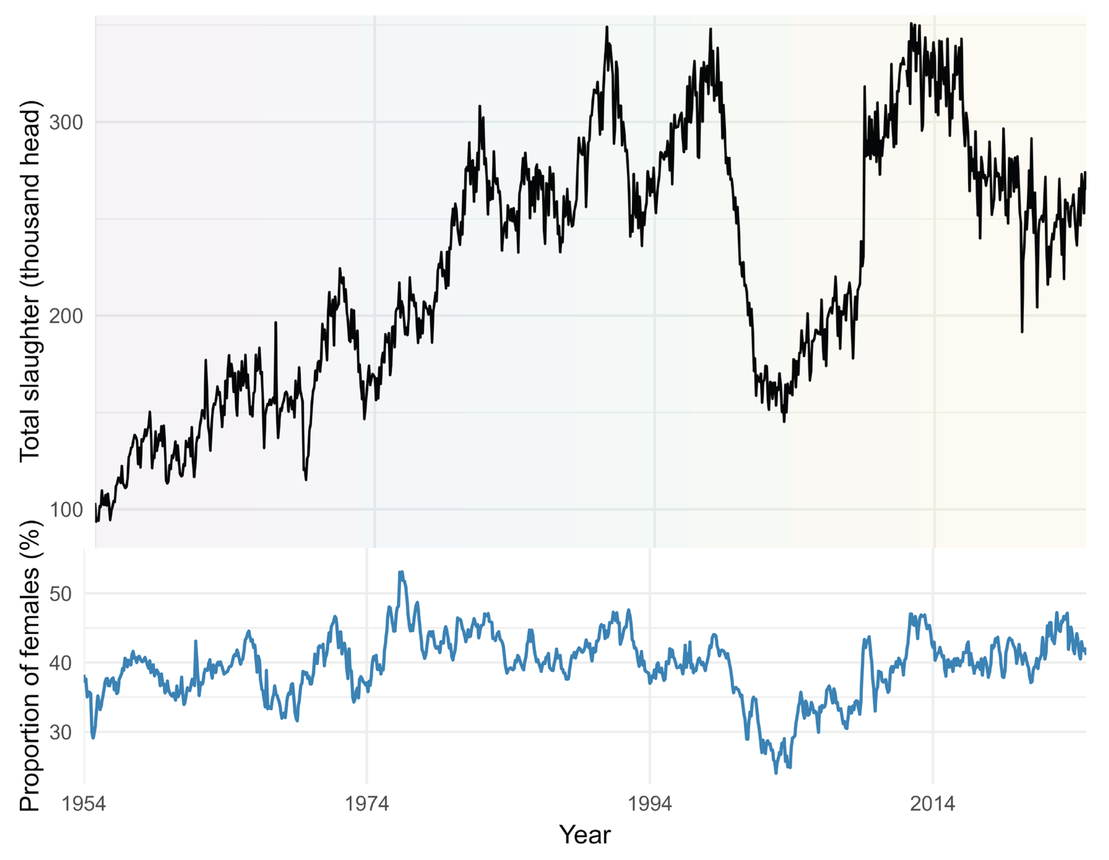
Figure 2.
Fit of the SARIMA(2,1,1)(1,0,1)12 model with intervention analysis — Observed vs. fitted series and standardised residuals. Note: Top panel: observed (grey) and fitted (blue) log(slaughter). Triangles: five statistically identified pulse outliers (Dec. 1966, Dec. 1968, Jan. 2009, Apr. 2020, May 2021). Bottom panel: standardised residuals with ±2σ bands. Source: authors’ calculations.
Figure 2.
Fit of the SARIMA(2,1,1)(1,0,1)12 model with intervention analysis — Observed vs. fitted series and standardised residuals. Note: Top panel: observed (grey) and fitted (blue) log(slaughter). Triangles: five statistically identified pulse outliers (Dec. 1966, Dec. 1968, Jan. 2009, Apr. 2020, May 2021). Bottom panel: standardised residuals with ±2σ bands. Source: authors’ calculations.
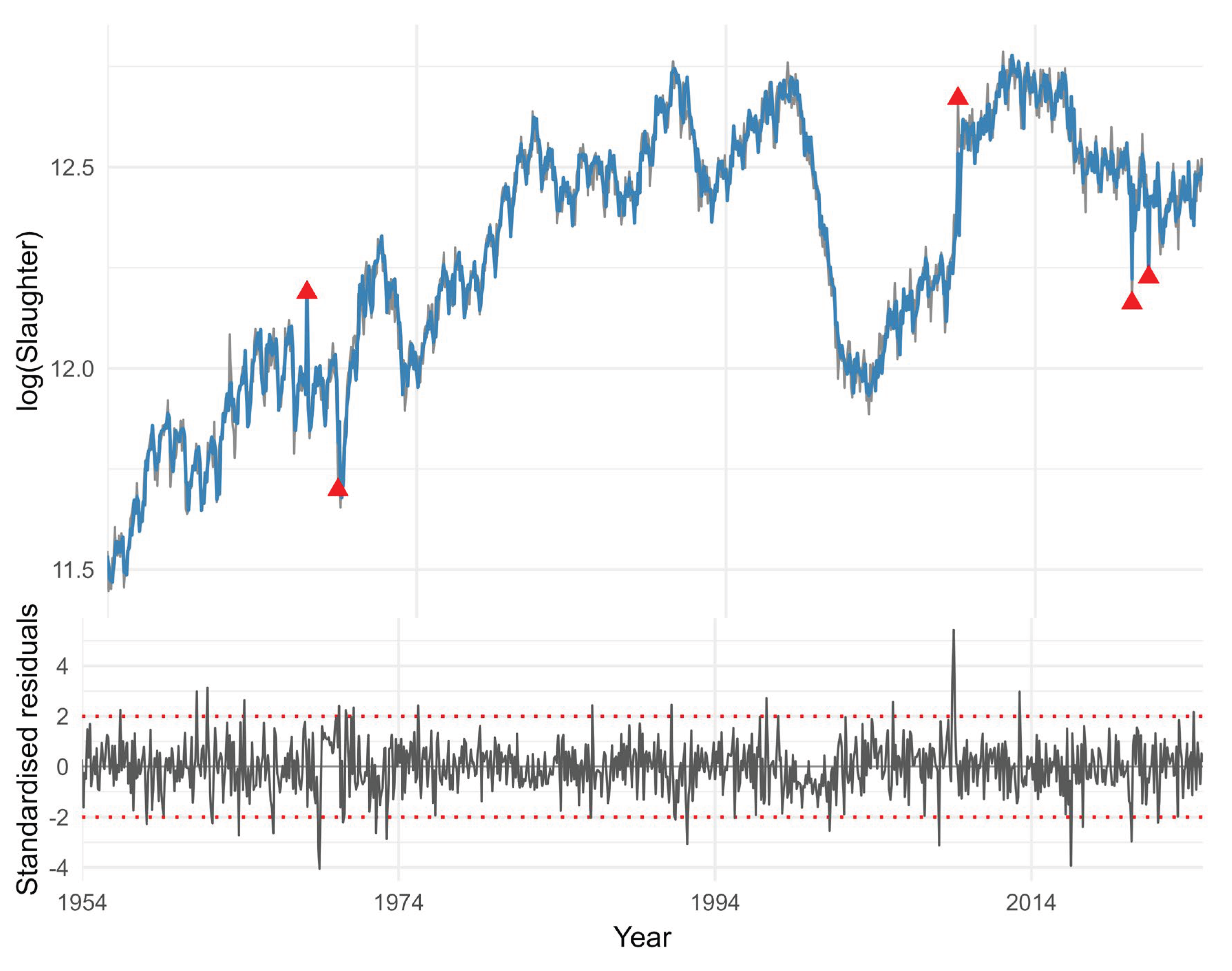
Figure 3.
Multitaper spectrum and Christiano-Fitzgerald cyclical component — Bovine slaughter, Colombia 1954–2024. Note: Left panel: spectral density (multitaper estimator, NW = 2.5; four tapers). Dotted lines indicate selected concentrations within the multimodal 4–8-year range, including peaks around 4.4–5.0 and 7.1–7.8 years. Right panel: cycle extracted using the Christiano-Fitzgerald filter (48–144 months). Source: authors’ calculations.
Figure 3.
Multitaper spectrum and Christiano-Fitzgerald cyclical component — Bovine slaughter, Colombia 1954–2024. Note: Left panel: spectral density (multitaper estimator, NW = 2.5; four tapers). Dotted lines indicate selected concentrations within the multimodal 4–8-year range, including peaks around 4.4–5.0 and 7.1–7.8 years. Right panel: cycle extracted using the Christiano-Fitzgerald filter (48–144 months). Source: authors’ calculations.
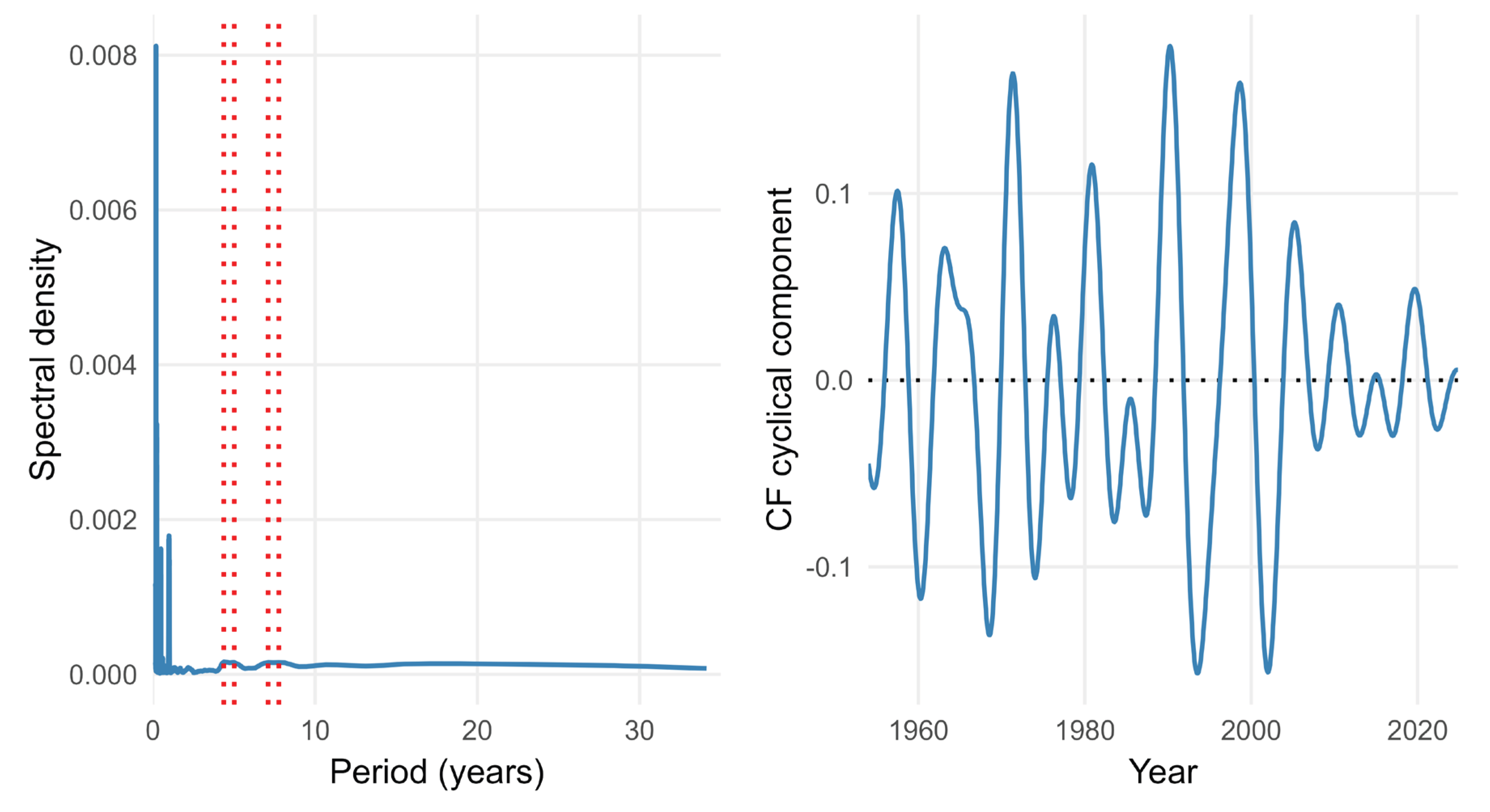
Figure 5.
Impulse-response function of cattle price to a unit shock in slaughter — VAR(1), Colombia January 1990–February 2000. Note: Solid line: mean response. Shaded band: 95% CI (bootstrap, 500 replications), which includes zero throughout the horizon shown. Horizontal axis: months. Source: authors’ calculations.
Figure 5.
Impulse-response function of cattle price to a unit shock in slaughter — VAR(1), Colombia January 1990–February 2000. Note: Solid line: mean response. Shaded band: 95% CI (bootstrap, 500 replications), which includes zero throughout the horizon shown. Horizontal axis: months. Source: authors’ calculations.
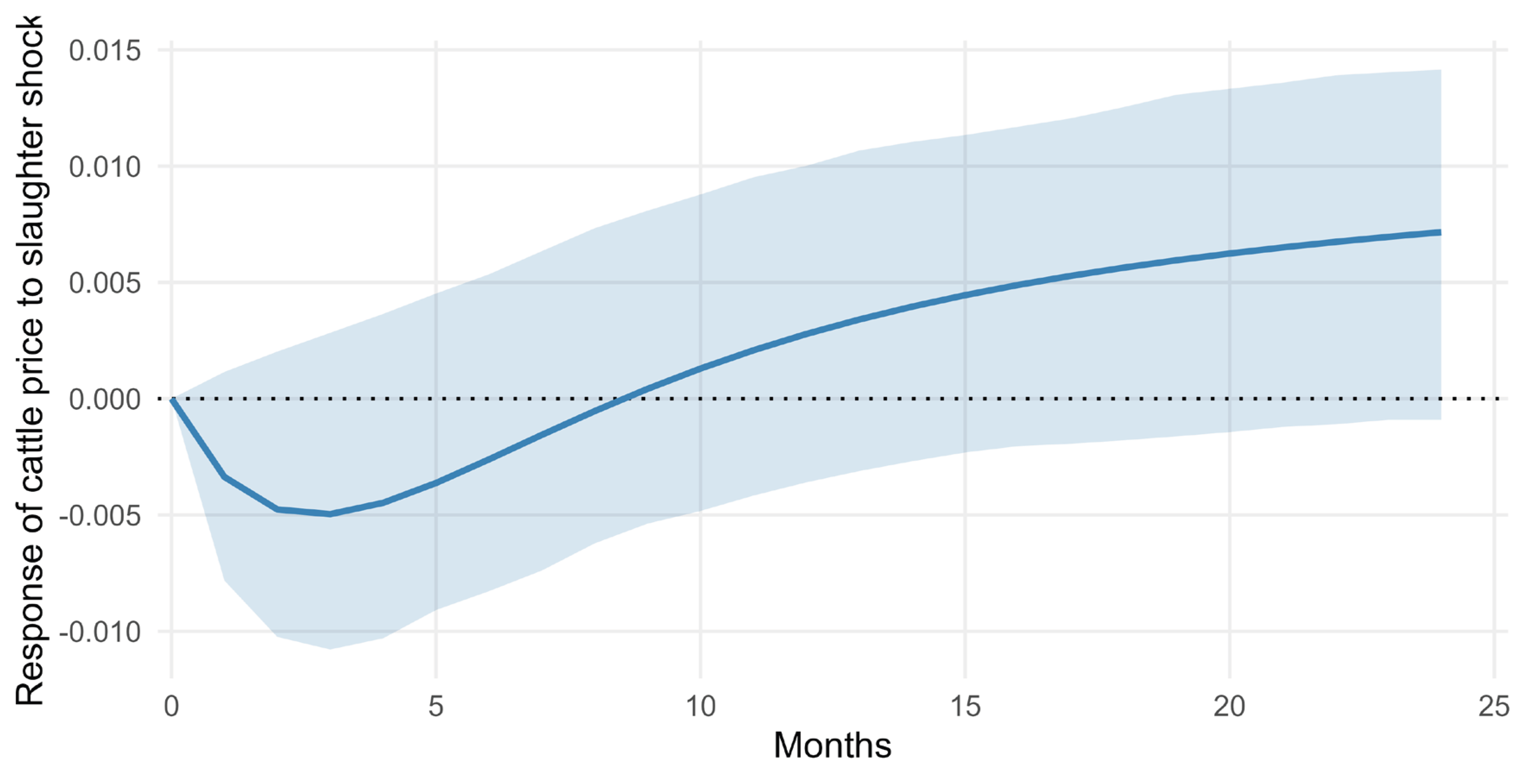
Figure 6.
Cross-correlation functions (CCF) of Δlog(slaughter) with changes in external variables — Colombia. Note: Top to bottom: CCF with changes in the ordinal ENSO index (1954–2024), policy interest rate (1995–2024), and ITCR-IPC-NT (1995–2024), each paired with Δlog(slaughter). The horizontal axis is plotted in years (±1 = ±12 months); Table 9 reports significant lags in months. Horizontal dotted lines: approximate 95% bands (±1.96/√T). External variables remain in their native measurement scales before differencing. Source: Banco de la República; NOAA/CPC. Authors’ calculations.
Figure 6.
Cross-correlation functions (CCF) of Δlog(slaughter) with changes in external variables — Colombia. Note: Top to bottom: CCF with changes in the ordinal ENSO index (1954–2024), policy interest rate (1995–2024), and ITCR-IPC-NT (1995–2024), each paired with Δlog(slaughter). The horizontal axis is plotted in years (±1 = ±12 months); Table 9 reports significant lags in months. Horizontal dotted lines: approximate 95% bands (±1.96/√T). External variables remain in their native measurement scales before differencing. Source: Banco de la República; NOAA/CPC. Authors’ calculations.
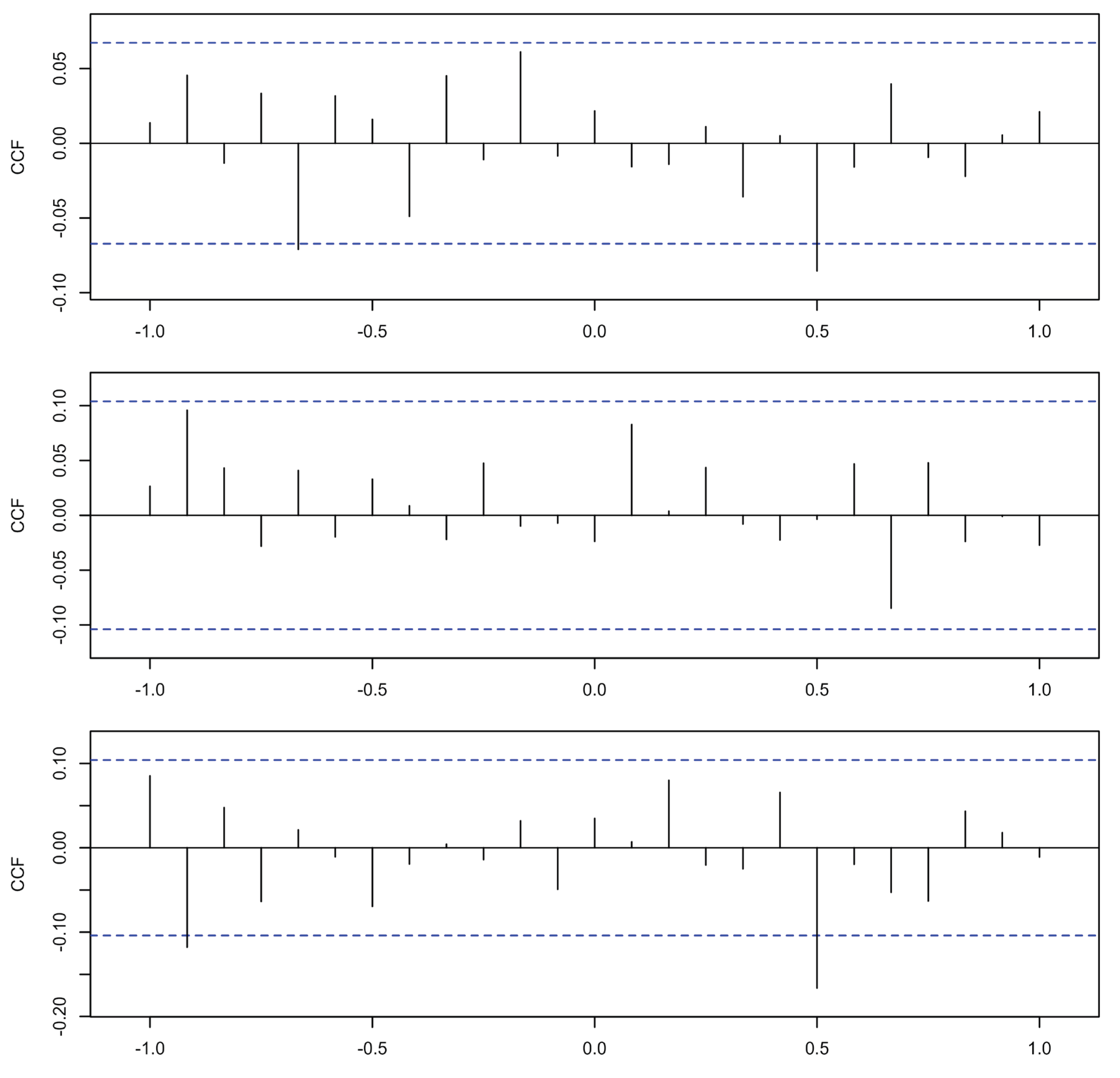
Figure 7.
Bovine inventory estimated via Kalman filter — Colombia, October 2008–December 2024.
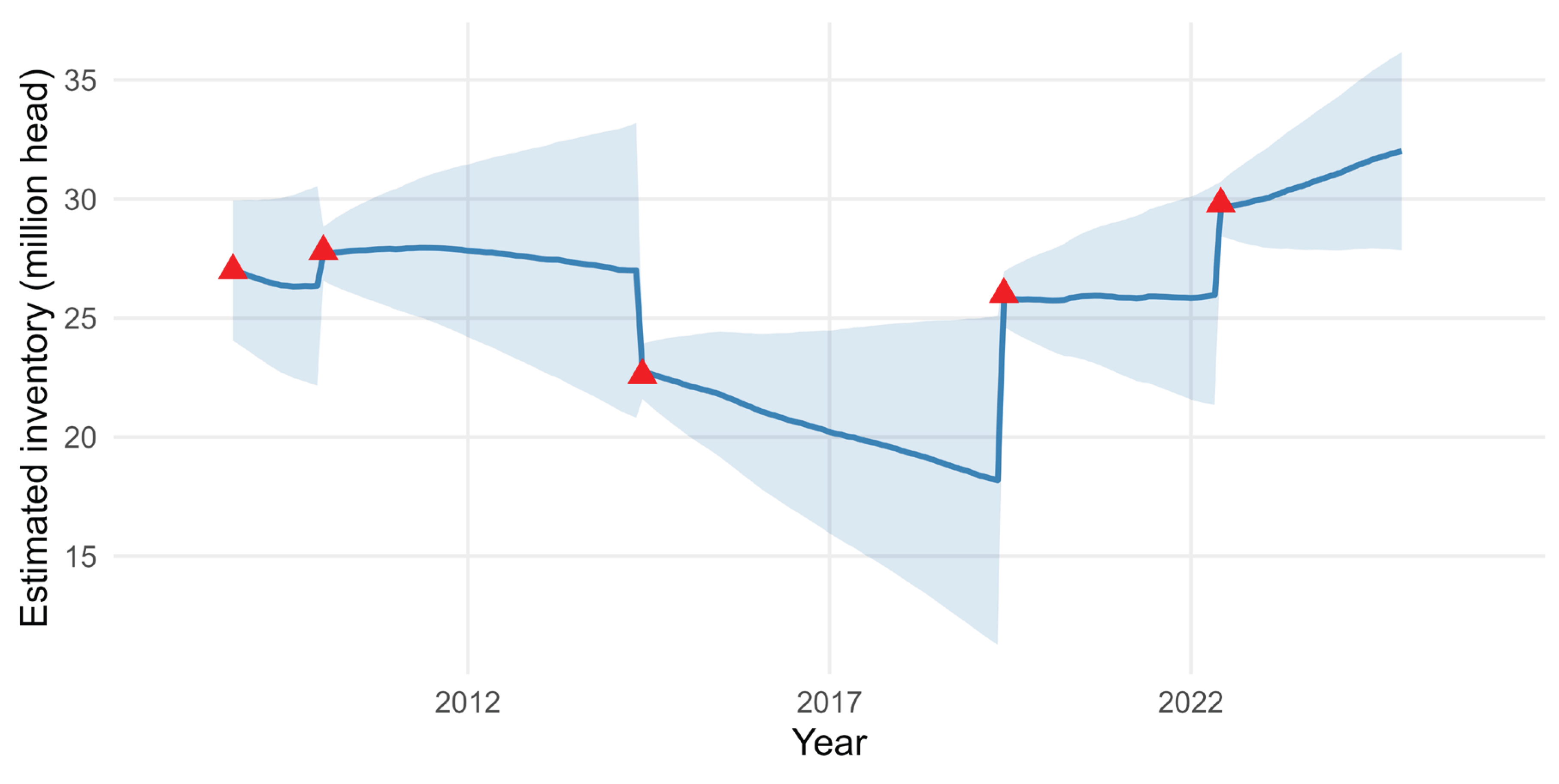
Figure 8.
Annualised implicit extraction rate — Colombia, 2008–2024. Note: Ratio of total monthly outflow (slaughter + live exports) to estimated inventory, annualised. Dotted line: period mean (14.9%). Bands: contraction phase (2012–2019, red) and expansion phase (2019–2024, green). Source: FEDEGAN. Authors’ calculations.
Figure 8.
Annualised implicit extraction rate — Colombia, 2008–2024. Note: Ratio of total monthly outflow (slaughter + live exports) to estimated inventory, annualised. Dotted line: period mean (14.9%). Bands: contraction phase (2012–2019, red) and expansion phase (2019–2024, green). Source: FEDEGAN. Authors’ calculations.
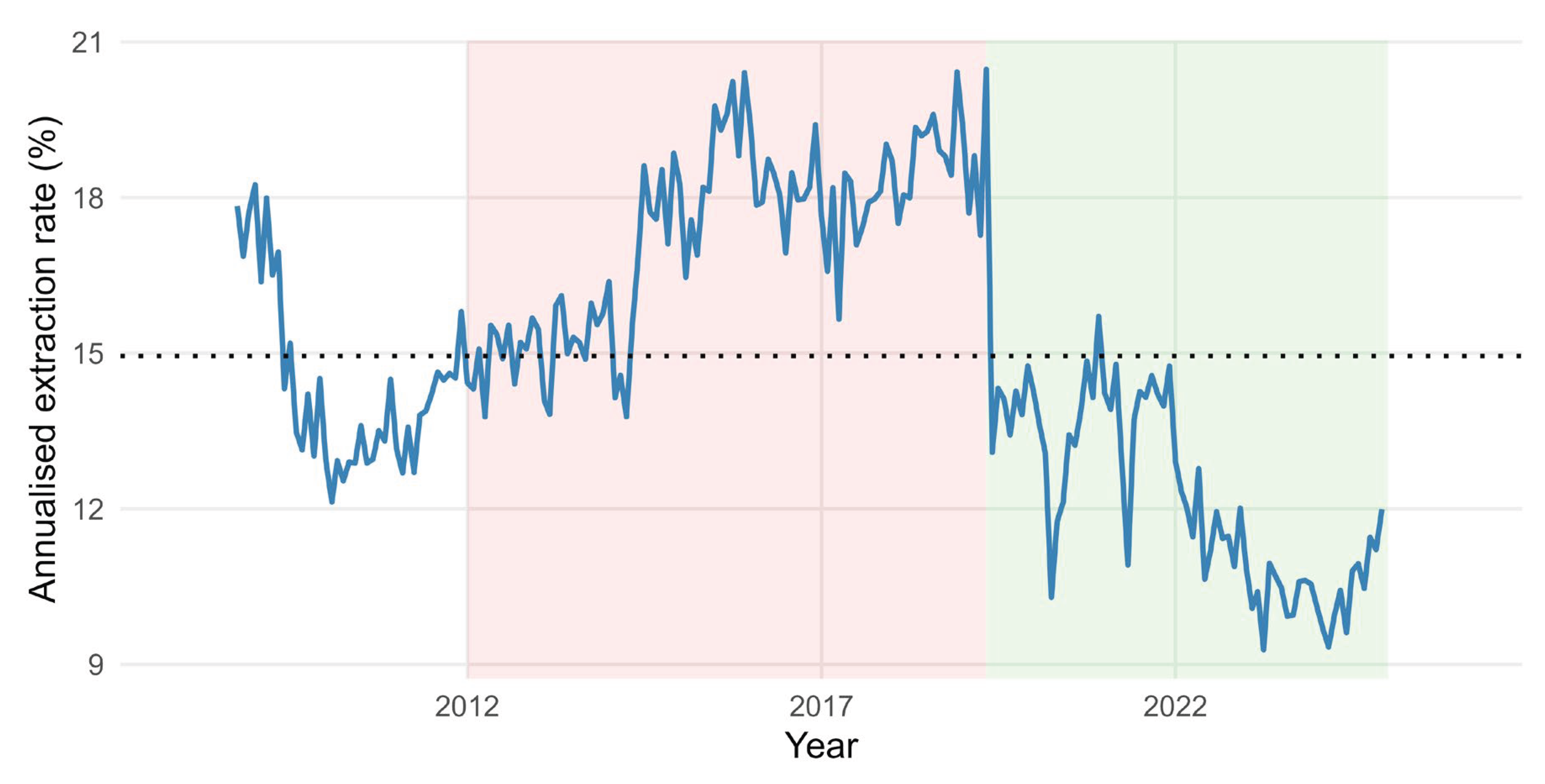
Figure 9.
Proportion of females in total slaughter — Colombia, October 2008–December 2024. Note: Solid line: monthly proportion. Dotted line at 50%: reproductive-collapse threshold. Dotted line at 39.5%: 1954–2024 historical mean. Thick blue line: 12-month moving average. Source: FEDEGAN; DANE-ESAG. Authors’ calculations.
Figure 9.
Proportion of females in total slaughter — Colombia, October 2008–December 2024. Note: Solid line: monthly proportion. Dotted line at 50%: reproductive-collapse threshold. Dotted line at 39.5%: 1954–2024 historical mean. Thick blue line: 12-month moving average. Source: FEDEGAN; DANE-ESAG. Authors’ calculations.
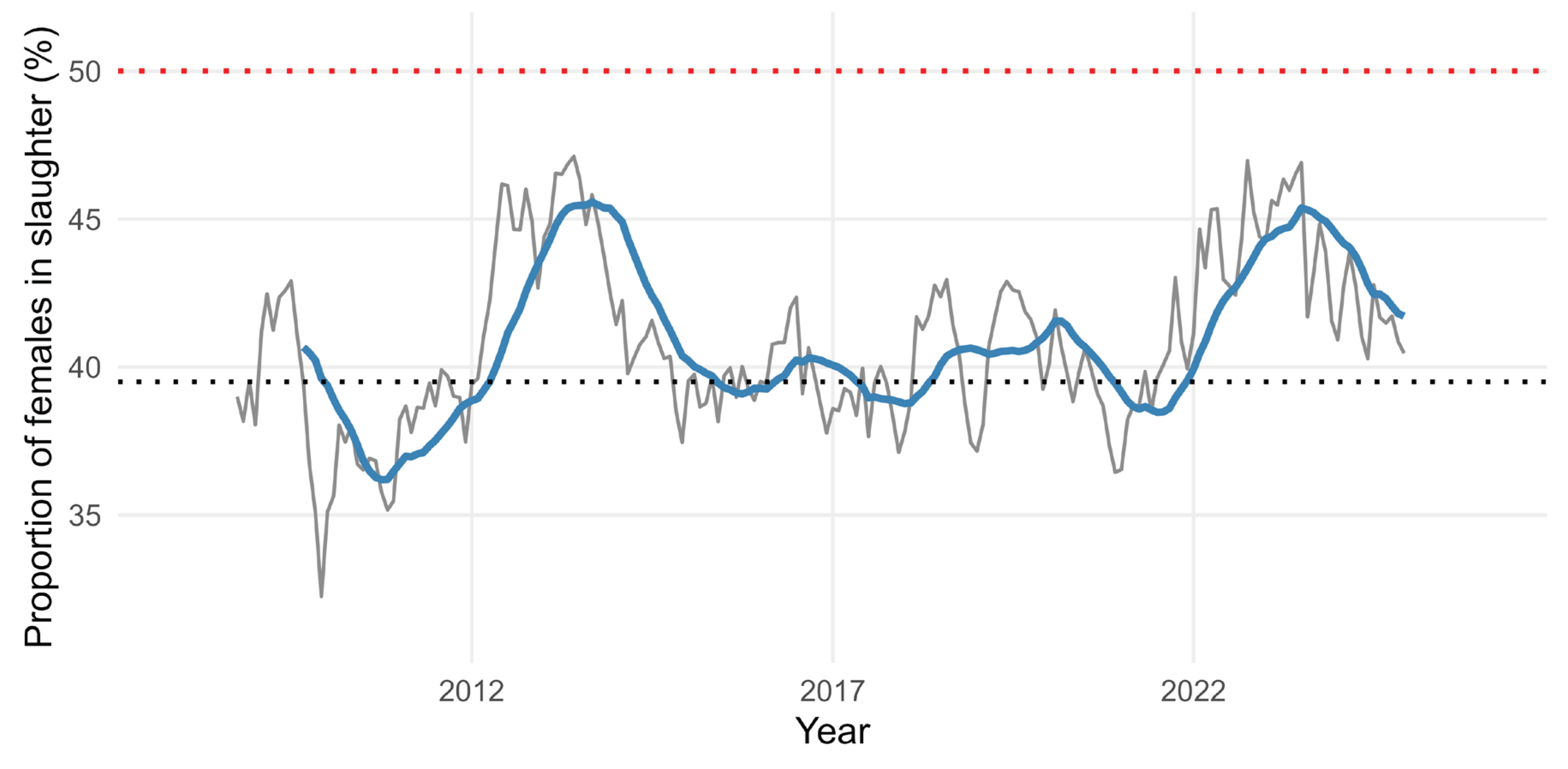

Table 1.
Parameters of the formal cattle-cycle model.
| Parameter | Definition |
|---|---|
| F(t) | Stock of breeding-age cows in period t |
| sf(t) | Number of females slaughtered in t |
| g | Fertility rate (calves born per breeding cow) |
| δ = 1 − μ | Survival factor (μ = mortality rate) |
| ab | Age at entry into breeding (in periods) |
| qt = pt − mt | Net return on sale: price less feeding cost mt |
| β = 1/(1+r) | Discount factor (r = real interest rate) |
| dt | Exogenous demand shock |
| Note: Source: authors’ elaboration based on [11] and [5]. | |
Table 2.
Data series used in the analysis.
| Variable | Period | Obs. | Source |
|---|---|---|---|
| Monthly bovine slaughter (total, female, male) | Jan 1954 – Nov 2024 | 851 | DANE-ESAG |
| Prices (cattle, poultry, pork, milk) — constant 1998 pesos | Jan 1990 – Feb 2000 | 122 | Medellín Livestock Fair; DANE |
| Monetary policy interest rate | Apr 1995 – Nov 2024 | 356 | Banco de la República |
| ITCR-IPC-NT (non-tradeables real exchange rate index) | Apr 1995 – Nov 2024 | 356 | Banco de la República |
| ENSO event index (ordinal, −3 to +1) | Jan 1954 – Nov 2024 | 851 | NOAA / CPC |
| Bovine inventory — monthly flows (slaughter + live exports) | Oct 2008 – Dec 2024 | 195 | FEDEGAN |
| Note: DANE = Departamento Administrativo Nacional de Estadística (National Administrative Department of Statistics); ESAG = Encuesta de Sacrificio de Ganado (Cattle Slaughter Survey); ITCR-IPC-NT = real exchange rate index deflated by the non-tradeables consumer price index; ENSO = El Niño–Southern Oscillation; NOAA = National Oceanic and Atmospheric Administration; CPC = Climate Prediction Center. All quantity and price series are natural-log transformed prior to analysis. | |||
Table 3.
Unit-root tests — Log(Total bovine slaughter), Colombia 1954-2024.
| Test | Statistic (level) | p-value (level) | Statistic (1st diff.) | p-value (1st diff.) |
|---|---|---|---|---|
| ADF (const. + trend) | −2.411 | 0.529 | −8.923 | < 0.010 |
| Phillips-Perron (const. + trend) | −2.318 | 0.467 | −42.716 | < 0.010 |
| KPSS (const. + trend) | 0.271 | < 0.010 | 0.043 | > 0.100 |
Note: ADF and PP: H0 = unit root. KPSS: H0 = stationarity. Source: authors’ calculations.
Table 4.
Comparison of ARIMA models — Log(Total bovine slaughter).
| Model | AICc | ΔAICc | Akaike weight | BIC |
|---|---|---|---|---|
| SARIMA(2,1,1)(1,0,1) [12] | −2,804.75 | 0.00 | 1.0000 | −2,776.38 |
| SARIMA(1,1,1)(1,1,1) [12] | −2,750.63 | 54.12 | 0.0000 | −2,727.04 |
Note: AICc = corrected Akaike information criterion. Search across 200 candidate specifications; top two shown. Source: authors’ calculations.
Table 5.
Coefficients of the SARIMA(2,1,1)(1,0,1) [12] model with intervention analysis.
Table 5.
Coefficients of the SARIMA(2,1,1)(1,0,1) [12] model with intervention analysis.
| Parameter | Estimate | Std. error | t | p-value |
|---|---|---|---|---|
| AR(1) | −0.854 | 0.099 | −8.589 | < 0.001 *** |
| AR(2) | −0.357 | 0.039 | −9.081 | < 0.001 *** |
| MA(1) | 0.456 | 0.104 | 4.403 | < 0.001 *** |
| SAR(1) | 0.996 | 0.002 | 530.830 | < 0.001 *** |
| SMA(1) | −0.916 | 0.016 | −55.215 | < 0.001 *** |
| Outlier Dec-1966 | +0.223 | 0.033 | 6.827 | < 0.001 *** |
| Outlier Dec-1968 | −0.171 | 0.034 | −5.233 | < 0.001 *** |
| Outlier Jan-2009 | +0.203 | 0.033 | 6.239 | < 0.001 *** |
| Outlier Apr-2020 | −0.197 | 0.034 | −5.958 | < 0.001 *** |
| Outlier May-2021 | −0.213 | 0.034 | −6.460 | < 0.001 *** |
Note: *** p < 0.001; * p < 0.05. AIC = −2,995.38 | BIC = −2,943.18. Estimation by exact maximum likelihood. Source: authors’ calculations.
Table 6.
Structural breaks in Colombian bovine slaughter — reference Bai-Perron specification.
| # | Date | 95% CI | Post-break trend | Associated historical event |
|---|---|---|---|---|
| 1 | Nov. 1965 | 1965(5)–1966(1) | +5.0% p.a. | Elimination of the rearing/fattening period |
| 2 | Dec. 1972 | 1972(11)–1973(3) | +5.9% p.a. | INCORA: improved-pasture expansion |
| 3 | Jun. 1980 | 1980(5)–1980(7) | −1.1% p.a. | Close of Lorente’s (1990) 4th cattle cycle (1976–1981) |
| 4 | Jun. 1988 | 1988(3)–1988(7) | −0.8% p.a. | Transition between Lorente’s 5th–6th cycles (1981–1990) |
| 5 | Aug. 1996 | 1996(7)–1996(9) | −13.6% p.a.* | Reference contraction shift; overlaps 1999 recession and DANE source discontinuity |
| 6 | Sep. 2003 | 2003(8)–2003(10) | +8.7% p.a. | Reference end of contraction regime; later dating is specification-sensitive |
| 7 | Dec. 2012 | 2012(11)–2013(1) | −2.8% p.a. | Reference break near onset of 2011–2019 contraction; exact late-sample date is specification-sensitive (Sec. 4.7) |
Note: Reference specification uses STL-aware imputation and a minimum regime length h = 85 months (≈10% of the sample); BIC selects seven breaks. Trend is the annualised slope in the subsequent reference regime. Conditional 95% break-date intervals are reported for this specification. Across nearby specifications, the first four dates move by at most 0–2 months, whereas the post-1990 dates are more sensitive (Section 4.4). QLR supF = 1,144.4 (p < 0.001). Source: authors’ calculations.
Table 7.
Predictive-causality tests — Monthly VAR(1) and Toda-Yamamoto robustness, Colombia January 1990–February 2000.
Table 7.
Predictive-causality tests — Monthly VAR(1) and Toda-Yamamoto robustness, Colombia January 1990–February 2000.
| Predictive direction | VAR(1) F | VAR(1) p | TY p | Interpretation |
|---|---|---|---|---|
| Cattle price → Slaughter | 5.206 | 0.0004 *** | 0.1774 | Baseline relation; not robust to TY |
| Slaughter → Cattle price | 3.311 | 0.0107 * | 0.5367 | Baseline relation; not robust to TY |
| Milk price → Slaughter | 3.556 | 0.0071 ** | 0.2143 | Baseline milk association; not robust to TY |
| Poultry price → Slaughter | 3.482 | 0.0080 ** | 0.1503 | Baseline poultry association; not robust to TY |
| Pork price → Slaughter | 2.085 | 0.0813 . | 0.1363 | Not significant at 5% in either test |
Note: Conventional VAR(1) p-values are from Granger F tests. Toda-Yamamoto uses an augmented VAR(2) (p = 1, dmax = 1) and tests only the first lag. *** p < 0.001; ** p < 0.01; * p < 0.05; . p < 0.10 for the conventional VAR(1) test. Cholesky identification is not used for these predictive-causality tests. Source: authors’ calculations.
Table 8.
Variance decomposition of Log(Slaughter) — VAR(1).
| Horizon | Own (%) | Cattle price (%) | Pork price (%) | Milk price (%) | Poultry price (%) |
|---|---|---|---|---|---|
| 1 month | 100.0 | 0.0 | 0.0 | 0.0 | 0.0 |
| 3 months | 91.9 | 2.0 | 2.3 | 3.7 | 0.1 |
| 6 months | 78.9 | 6.7 | 6.5 | 7.8 | 0.1 |
| 12 months | 70.5 | 12.2 | 9.4 | 7.8 | 0.1 |
| 18 months | 67.4 | 14.7 | 9.6 | 8.0 | 0.3 |
| 24 months | 65.2 | 15.8 | 9.4 | 8.4 | 1.1 |
Note: Rows sum to 100%. Baseline Cholesky ordering: cattle price → slaughter → poultry price → pork price → milk price. Across four total orderings (baseline plus three alternatives), the 24-month own share ranges from 63.6% to 65.2% and the cattle-price share from 14.6% to 15.9%; pork ranges from 8.6% to 9.4%, milk from 7.4% to 8.7%, and poultry from 1.1% to 4.6%. Source: authors’ calculations.
Table 9.
Summary: external-shock protocol for bovine slaughter.
| Variable | Window | Sig. CCF lag | Granger predictive p-val. | ΔAIC vs. base | LRT p-val. | Conclusion |
|---|---|---|---|---|---|---|
| Climate (ordinal ENSO index) | 1954–2024 | −8, +6 (r=−0.09, −0.08) | 0.912 | +1.85 | 0.698 | CCF-only association; no robust incremental predictive content |
| Interest rate | 1995–2024 | None | 0.731 | +1.92 | 0.783 | No discernible effect |
| ITCR-IPC-NT | 1995–2024 | −11, +6 | 0.480 | +1.30 | 0.404 | No discernible effect |
| Interest rate + ITCR (joint) | 1995–2024 | — | — | +3.53 | 0.788 | No joint effect |
Note: Baseline model SARIMA(2,1,1)(1,0,1) [12]: AIC = −1,071.91 (1995–2024 window). A positive ΔAIC indicates deterioration. Source: authors’ calculations.
Table 10.
Estimated bovine herd inventory and outflows — Colombia, 2008–2024.
| Year | Avg. herd (M) | Slaughter (M) | Exports (M) | Total outflow (M) | Extraction rate (%) | % females slaughtered |
|---|---|---|---|---|---|---|
| 2008* | 26.9 | 1.085 | 0.092 | 1.176 | 17.5 | 38.9 |
| 2009 | 26.4 | 3.823 | 0.232 | 4.056 | 15.3 | 39.6 |
| 2010 | 27.8 | 3.624 | 0.017 | 3.641 | 13.1 | 36.5 |
| 2011 | 27.9 | 3.900 | 0.011 | 3.910 | 14.0 | 38.8 |
| 2012 | 27.7 | 4.124 | 0.014 | 4.138 | 14.9 | 43.5 |
| 2013 | 27.3 | 4.055 | 0.114 | 4.169 | 15.3 | 45.4 |
| 2014 | 24.4 | 3.983 | 0.045 | 4.027 | 16.6 | 40.4 |
| 2015 | 21.8 | 3.987 | 0.069 | 4.056 | 18.6 | 39.3 |
| 2016 | 20.7 | 3.652 | 0.134 | 3.786 | 18.3 | 40.1 |
| 2017 | 19.9 | 3.408 | 0.110 | 3.517 | 17.7 | 38.8 |
| 2018 | 19.0 | 3.435 | 0.148 | 3.583 | 18.9 | 40.6 |
| 2019 | 22.7 | 3.408 | 0.122 | 3.530 | 15.9 | 41.0 |
| 2020 | 25.8 | 3.257 | 0.198 | 3.455 | 13.4 | 39.4 |
| 2021 | 25.9 | 3.302 | 0.282 | 3.584 | 13.9 | 39.5 |
| 2022 | 28.2 | 3.107 | 0.194 | 3.301 | 11.8 | 44.1 |
| 2023 | 30.5 | 3.086 | 0.074 | 3.159 | 10.4 | 44.7 |
| 2024 | 31.6 | 3.226 | 0.090 | 3.316 | 10.5 | 41.7 |
Note: Avg. herd = average annual estimated monthly inventory (million head). Slaughter, exports, and total outflow in million head per year. Extraction rate = (total outflow / estimated herd) × 100, annualised. * 2008: October–December only (3 months). Source: FEDEGAN and ICA. Authors’ calculations.
Disclaimer/Publisher’s Note: The statements, opinions and data contained in all publications are solely those of the individual author(s) and contributor(s) and not of MDPI and/or the editor(s). MDPI and/or the editor(s) disclaim responsibility for any injury to people or property resulting from any ideas, methods, instructions or products referred to in the content. |
© 2026 by the authors. Licensee MDPI, Basel, Switzerland. This article is an open access article distributed under the terms and conditions of the Creative Commons Attribution (CC BY) license (http://creativecommons.org/licenses/by/4.0/).
Copyright: This open access article is published under a Creative Commons CC BY 4.0 license, which permit the free download, distribution, and reuse, provided that the author and preprint are cited in any reuse.