
Submitted:
02 October 2026
Posted:
07 October 2026
You are already at the latest version
Abstract
Air quality indices, severity ratings, and similar series come as ordered categories, yet standard forecasting methods produce continuous predictions. We propose a two-stage approach using NeuralProphet, which decomposes a series into trend, seasonality, and autoregressive components. In the first stage, NeuralProphet is fit to the ordinal labels treated as continuous, yielding a decomposition and a continuous forecast. In the second, ordered thresholds mapping it to categories are optimized on a validation segment, replacing naive rounding. We evaluate on a controlled simulation and two real series, Beijing air quality and electricity load in a Ball State University building. On the simulation, the method recovers the latent ordering and generating components despite being fit on discretized labels, and threshold optimization improves the quadratic weighted kappa over rounding by 0.05 to 0.08, and by more when a miscalibrated trend leaves the ordering intact but the level off. On the real series it leads at every horizon, reaching a kappa of 0.57 on air quality and 0.89 on building load at 72 hours, and the gain grows with the horizon on air quality. The fitted components match each series’ structure. The approach is therefore an effective, interpretable framework for ordinal forecasting without specialized machinery.
Keywords:
ordinal time series
; forecasting
; NeuralProphet
; air quality prediction
; threshold optimization
; time series decomposition
1. Introduction
Time series forecasting is a fundamental problem in statistics and machine learning, with applications ranging from demand prediction to environmental monitoring. While extensive research has focused on forecasting continuous outcomes, some series are recorded as ordinal responses, where outcomes fall into ordered categories. Examples include air quality indices (e.g., Good, Moderate, Unhealthy), customer satisfaction ratings, disease severity stages, and activity intensity levels.
Traditional approaches to ordinal time series forecasting include ordinal regression models extended with autoregressive components [6] and hidden Markov models with ordinal emissions [7]. Both are specialized models requiring dedicated estimation machinery, and neither yields the interpretable decomposition a general-purpose forecaster provides. A simpler alternative is to forecast the labels continuously and discretize the result [8]. This keeps access to general-purpose forecasters, but it is typically implemented by rounding to the nearest integer, leaving the placement of the cut-points untuned. Our approach starts here and replaces the rounding with thresholds fitted to the data.
NeuralProphet [3] is a neural forecasting framework that extends the classical Prophet model with autoregressive components and lagged regressors, and that decomposes a series into interpretable additive components (Section 2.2).
In this paper, we propose a two-stage approach for ordinal time series forecasting. In the first stage, NeuralProphet is applied to the ordinal data treated as continuous, producing an interpretable decomposition and a continuous forecast. In the second stage, the continuous forecast is mapped to ordinal categories through a set of ordered thresholds optimized on a validation segment, rather than by naive rounding. We demonstrate that this approach recovers the underlying structure of the data and improves predictive accuracy over rounding across simulated and real datasets.
Our contributions are as follows:
- 1.
- We propose a two-stage method that combines NeuralProphet’s interpretable decomposition with validation-set threshold optimization for mapping continuous forecasts to ordinal categories.
- 2.
- Using a controlled simulation with a known generating process, we demonstrate that the method recovers both the latent ordering and the underlying component structure despite being fit on discretized labels.
- 3.
- We evaluate the method on two real ordinal time series spanning environmental and infrastructure domains, assessed with an expanding-window evaluation.
- 4.
- We show that threshold optimization consistently improves predictive accuracy over naive rounding, and that the gain is largest where the first-stage forecast is miscalibrated but order-preserving.
The remainder of this paper is organized as follows. Section 2 reviews related work on ordinal time series and NeuralProphet. Section 3 describes our methodology. Section 4 presents experimental results on simulated data and two real datasets. Section 5 discusses findings and limitations. Section 6 concludes.
2. Related Work
2.1. Ordinal Time Series Models
Ordinal regression models, particularly the cumulative link model [5,19], provide the statistical foundation for analyzing ordered categorical outcomes. The proportional odds model assumes a common effect of predictors across category thresholds, yielding parsimonious and interpretable models. Extensions to time series settings require incorporating autoregressive components, typically by including lagged responses as covariates.
Chen and Chiu [8] presented one of the few studies explicitly addressing ordinal time series forecasting, applying four methods to daily air quality index prediction across sixteen cities and counties in Taiwan: (1) an autoregressive model with exogenous variables and GARCH errors, (2) autoregressive multinomial logistic regression, (3) support vector machine classification, and (4) neural network autoregression. Seasonality was handled through monthly dummy variables, and the models used three weather covariates: precipitation and temperature entered at a one-day lag, while wind direction entered through an hour-lag nowcasting effect, treating its near-term value as available at forecast time. Forecasts were produced one step ahead under a rolling-window scheme, re-estimating each model on a fixed-length recent window and predicting the next day’s level. A consequence of this design is that the lagged response entering each prediction is the actual observed category from the previous day, so each forecast is conditioned on the true recent history. Our setting is more demanding. We make blind multi-step forecasts in which the target’s own past values are not observed over the forecast horizon, so the autoregressive terms beyond the forecast origin must be filled with the model’s own predictions rather than with observed responses. A one-step-ahead forecast made with observed lags and a blind multi-step forecast are different forecasting problems, the latter being harder because errors accumulate through the autoregressive recursion rather than being reset by each new observation. We return to this distinction in Section 4.2.4.
Outside the time series setting, ordinal outcomes have a substantial machine learning literature, surveyed by Gutiérrez et al. [20], in which a recurring strategy is to reduce the ordinal problem to simpler ones rather than model it directly [21]. Our two-stage approach is a reduction of that kind, applied to forecasting.
Recent work has produced R packages for ordinal time series analysis. The otsfeatures package [9] provides tools for feature extraction, clustering, and classification of ordinal time series, while ctsfeatures [10] addresses the more general categorical (nominal) case. However, these packages focus on characterizing and comparing existing series rather than forecasting future values. Weiß and colleagues have developed specialized models for discrete-valued series [18], including soft-clipping autoregressive (scAR) models [11] and discrete ARMA processes, which are tailored to particular ordinal structures and require model-specific estimation machinery.
Existing approaches to ordinal time series forecasting are therefore either specialized models requiring dedicated estimation methods, or ad hoc treatments in which ordinal data are handled continuously and rounded. Practitioners are left to either manually implement AR ordinal logistic models with seasonal dummy variables or apply standard continuous forecasting methods without accounting for the ordinal structure. Our work addresses this gap by demonstrating that a general, interpretable decomposition-based forecaster, NeuralProphet, can be adapted to ordinal outcomes through validation-set threshold optimization, using widely available software rather than model-specific machinery.
2.2. NeuralProphet
NeuralProphet [3] extends the Prophet model [4] by incorporating neural network components for autoregressive modeling and lagged regressors. Like Prophet, NeuralProphet decomposes time series into interpretable additive components: a piecewise-linear trend with learnable changepoints, Fourier-based seasonality at multiple frequencies, holiday and event effects, and covariate regressors.
The key extensions over Prophet include: (1) autoregressive modeling via a feedforward neural network that processes lagged target values, (2) lagged regressor handling that allows covariates to influence predictions through their recent history, and (3) global modeling capability for multiple related time series.
For seasonality, NeuralProphet uses Fourier series representations:
where P is the period (e.g., 24 for daily, 7 for weekly) and N controls the flexibility. This is more parsimonious than dummy encoding, which needs parameters per seasonal cycle. For hourly data with daily and weekly patterns, that is Fourier coefficients per cycle against 29 dummy variables (23 hourly plus 6 day-of-week).
3. Methodology
3.1. Problem Formulation
Let be an ordinal time series where represents ordered categories, and let with be an accompanying covariate series. We observe both for , with the first T steps used to fit and tune the model and the remaining N steps held out as the test set on which we report metrics. To allow threshold tuning without contaminating the test set, the in-sample window is further split chronologically into a training block and a validation block. The model is fit on the two blocks combined, and the validation block is additionally reused to tune the category thresholds (Section 3.5). The test block is used by neither the forecaster nor the threshold optimizer.
The model must forecast without ever observing the true values. The covariates, in contrast, are treated as exogenous and known throughout, including the test window. This is the natural setting whenever future covariate values can be anticipated, either from an external forecast (numerical weather prediction, for meteorological covariates) or because they are fixed in advance (calendar effects, scheduled events, controlled inputs). They are supplied to the model as inputs rather than forecast by it.
Forecasts are produced in a rolling-origin multi-step fashion. At each forecast origin the model emits a block of steps at once, then the origin advances by B and the procedure repeats until the full forecast horizon is covered. We detail this loop in Section 3.3.
3.2. NeuralProphet Model
NeuralProphet models the time series as a sum of additive components:
where is the trend (piecewise-linear with learnable changepoints), captures Fourier-based seasonality, is the autoregressive component with lags of the target, is the lagged-regressor component with lags of the covariate vector (set independently of , subject to ), and is the future-regressor component, contributing the contemporaneous value at the time being predicted. The future regressor requires the covariate’s future values to be known, exactly as assumed in Section 3.1. Together, the lagged and future regressors give the model access to a distributed lag of the exogenous covariates at every forecast step, capturing both delayed effects (such as pollutant accumulation over preceding hours) and instantaneous effects.
We treat the ordinal categories as continuous numeric values during fitting, and NeuralProphet minimizes a smooth (Huber) loss [16] between and the observed integer labels. We denote the resulting continuous forecast at time t by and reserve for the final ordinal prediction obtained by thresholding in the next subsection.
Treating ordinal categories as continuous in this way is deliberately misspecified. The integer labels carry only order, not a cardinal scale, so fitting them with a continuous regressor under a symmetric Huber loss assumes a metric structure and an error distribution that the data need not possess. The approach does not rely on these assumptions holding. It requires only that the continuous forecast preserve the ordering of the response, so that an order-preserving threshold mapping can recover the categories. The thresholding stage (Section 3.4) and its optimization (Section 3.5) then absorb the unequal spacing between categories and the regression-to-the-mean induced by the symmetric loss. Section 4.1.4 demonstrates the required monotonicity directly, using a simulation in which the underlying continuous variable is known.
3.3. Rolling-Origin Multi-Step Forecasting
Equation (2) describes a single one-step prediction. NeuralProphet generalizes this to a multi-step forecast by emitting B consecutive predictions from one input window: given , the lagged covariates , and the future-regressor values , the model outputs the block in a single pass. We refer to B as the output block width. It corresponds to NeuralProphet’s n_forecasts setting and is distinct from the forecast horizon H defined below. Within a block this is a direct multi-step strategy. The model is trained on the multi-step objective and the B predictions are produced in a single pass, with no prediction fed back as an input. Across blocks the scheme is recursive, since each new origin is supplied with the preceding block’s predictions, so error still accumulates, but once every B steps rather than at every step. Empirical comparisons of multi-step strategies for machine learning forecasting models have generally favored direct over recursive approaches, particularly at longer horizons [2].
A single block reaches only B steps ahead. NeuralProphet emits that block natively but does not extend beyond it, so the rolling-origin loop described below, in which the model’s own predictions fill the autoregressive input past the origin, is implemented here. To cover a horizon of steps we chain blocks as illustrated in Figure 1 for the case . Throughout our experiments the horizon spans the entire held-out test block, so . The first origin is , where the AR input window consists entirely of true training values. After the first block of B steps is produced, the origin advances by B steps, and the procedure repeats. The horizon is therefore covered by successive chunks (the final chunk is padded if H is not a multiple of B). The two input pathways are filled differently across chunks, reflecting what is and is not known.
For the target (y) pathway, the AR input window contains true observed values for timestamps , and the model’s own previous continuous predictions for timestamps . The model is therefore blind to the future target throughout the forecast window. By chunk the AR input consists entirely of fed-back predictions (shown by the red bracket in Figure 1), and the AR pathway accumulates error chunk over chunk. With the and used throughout, this is chunk 3, so the forecast is fully blind from step 25 of the horizon onward. At there is a single chunk and no feedback at all. This is the standard blind multi-step setup. For the covariate () pathway, the lagged- and future-regressor input windows are populated with real observations for timestamps and with the externally supplied future covariate values for timestamps (the inputs described in Section 3.1; the blue bracket in Figure 1 marks chunk 1’s future-regressor inputs as a representative example). The covariate pathway does not feed back model outputs at any point. Covariates are exogenous and the model never tries to forecast them.
The asymmetry between the two pathways is intentional and matches the assumption in Section 3.1. Future covariate values are known (or supplied by an external forecast), while future target values are not. The validation segment is forecast under the same rolling-origin multi-step procedure used for the test set, so the predictions used for threshold tuning are generated in the same way as those used for final evaluation, differing only in that the model has been fit on the validation segment as well (Section 3.5.4).
Table 1 collects the configuration symbols introduced above, together with those used in the sections that follow.
3.4. Ordinal Conversion via Thresholding
We map the continuous forecast to an ordinal category through a set of ordered cut-points :
with the conventions and .
The simplest choice places the cut-points at the integer midpoints, , which recovers the baseline rounding rule
This baseline implicitly assumes that the continuous forecast is symmetrically distributed within each category and that adjacent category boundaries on the underlying latent scale are equally spaced. Both assumptions can fail in practice. The Beijing AQI categories used in our experiments illustrate the unequal-spacing issue directly. They are defined by PM2.5 cut-points at 35, 75, and [1], so successive gaps on the underlying concentration scale are 40 and , which are markedly unequal. The symmetry assumption fails for two further reasons. NeuralProphet’s Huber objective shrinks predictions toward the mean, so imbalanced category frequencies leave asymmetrically distributed within a category, and drift over the test window shifts its location relative to the fixed midpoints. We therefore treat as parameters to be learned from a validation segment, a procedure we refer to as threshold optimization and describe in Section 3.5.
3.5. Threshold Optimization
3.5.1. Objective
We tune the thresholds to maximize Cohen’s quadratic weighted kappa, , on a validation segment. Section 3.6 defines and motivates the choice. Given continuous validation forecasts and the corresponding true ordinal labels :
where is obtained by applying (3) to . Because is integer-valued and changes only when a threshold crosses a data point, is piecewise constant in with discontinuities at those crossings. Its gradient is therefore zero almost everywhere and undefined at the jumps, so gradient-based methods are unusable without resorting to a smooth surrogate that changes the objective. We instead use the derivative-free Nelder–Mead simplex algorithm [15], which operates directly on function values and is well suited to objectives of this form.
3.5.2. Reparameterization
Direct optimization over subject to the ordering constraint is awkward, since enforcing the constraint by sorting inside the objective introduces discontinuities in the search landscape. We instead reparameterize the thresholds in terms of unconstrained gap parameters :
where the gap function maps each parameter to a strictly positive gap, so the ordering is satisfied automatically and the optimizer searches an unconstrained space with a smooth landscape suited to Nelder–Mead. We use the softplus function, , which maps onto and places no upper bound on the gaps, allowing the thresholds to spread as far apart as the data require. A bounded alternative that caps each gap (for example a scaled sigmoid with a user-specified maximum gap M) could in principle regularize the solution and discourage degenerate configurations in which a category is never predicted, but we found this unnecessary in practice. With enough random restarts the unbounded softplus parameterization converges to the same or nearly the same thresholds, so we adopt it throughout and avoid the additional hyperparameter M.
3.5.3. Multi-Start Search and top-m Averaging
Because the kappa surface is non-convex and piecewise constant, the optimizer can converge to suboptimal local maxima depending on initialization. We therefore run Nelder–Mead from S starting points: one at the evenly spaced initialization and random initializations drawn uniformly from the range of . To stabilize the solution against optimizer noise, we sort the S converged threshold vectors by their validation kappa, keep the top m, and report the elementwise mean as the final . This borrows the rank-and-average mechanic of Ordinal Forests [13], which generates many random score sets for the ordinal categories and averages the top-ranked ones, with the same goal of reducing sensitivity to any single run. We apply it to threshold vectors recovered after fitting rather than to score sets used during fitting. The optimized thresholds are then applied through (3) to the test set forecasts, with no further tuning, to produce the final ordinal predictions.
3.5.4. Use of the Validation Block
The continuous validation forecasts in Equation (5) are produced as follows. The model is fit once on the training and validation blocks combined, and this single fitted model supplies both the validation-block predictions used to tune the thresholds and the test-block forecast used for evaluation. The validation block is therefore used twice, once as part of the data the forecaster is fit on and once to select the thresholds, while the test block is held out from both stages.
This design is deliberate. The validation block is the segment immediately preceding the test window, and in a time series it is the most recent and most predictive history available. A strict train/validation/test partition would exclude exactly the observations adjacent to the test set, forcing the forecaster to extrapolate from a more distant origin. Including it also makes the two stages coherent, since the thresholds are calibrated on predictions from the same model that produces the test forecast rather than from a separate model fit on less data. No test observation is used to fit the model or to choose a threshold, so the reported metrics remain genuinely out-of-sample. The validation predictions are in-sample, however, and so somewhat more accurate than the test forecasts the thresholds are eventually applied to. Section 5 returns to this.
3.6. Evaluation Metrics
We evaluate ordinal predictions on the held-out test set using:
- Quadratic weighted kappa () [12]: a measure of agreement between predicted and actual categories with quadratic penalties on the distance between them. Two properties make it well suited to ordinal classification. It is chance-corrected, so a model that predicts only the dominant class is not credited for accidental matches, and the quadratic weighting respects ordinal structure, penalizing an error of two categories four times as heavily as an error of one. Both weighted kappas share these two properties. We optimize the thresholds against the quadratic form (Section 3.5) because its heavier penalty on distant errors matches the cost structure of the applications we consider, where a two-category miss is far more consequential than two adjacent-category misses. The remaining metrics are reported for comparison.
- Linearly weighted kappa (): like but with penalties proportional to category distance rather than its square. It is chance-corrected and respects ordinal structure, but weights large and small errors less disparately. We report it for comparison but do not optimize against it.
- Exact accuracy: proportion of exactly correct predictions, . It is neither chance-corrected nor sensitive to ordinal structure, treating all errors as equivalent.
- Within-one accuracy: proportion of predictions within one category of the true value, . It reflects ordinal structure coarsely, distinguishing only small errors from large ones, and is not chance-corrected.
- Mean absolute error (MAE): , treating categories as integers. It respects ordinal structure by penalizing errors linearly with category distance, but is not chance-corrected.
We report all metrics for both the baseline rounding rule and the threshold-optimized predictions to isolate the contribution of threshold tuning.
On the real series we do not report a fold-wise standard deviation for . Cohen’s kappa is chance-corrected, so on a fold spanning only two categories the expected-disagreement denominator is small and the statistic swings on a handful of observations. At the shortest horizons it is undefined outright on the folds whose observed or predicted categories never change, which do occur in these data. We therefore concatenate the paired predictions and observations across the non-overlapping origins at a given horizon and compute a single pooled on that concatenated table. Accuracy and MAE, which are stable on such folds, are pooled in the same way so that every metric on a horizon is computed from the same set of hours.
4. Experiments
4.1. Simulated Data
4.1.1. Motivation
On real data the true generating mechanism is unobserved, so we cannot separate the quality of the continuous forecast from the calibration of the threshold mapping or the strength of the ordinal signal. We therefore complement the real-data experiments with a controlled simulation in which the entire generating process (trend, seasonality, covariate effects, autocorrelation, and the thresholds that map a latent variable to ordinal categories) is specified in advance. Knowing the ground truth lets us ask whether the additive decomposition recovers the true components, which real data cannot answer (Section 4.1.4), and lets us vary the difficulty of the problem in controlled ways (Section 4.1.5).
The simulation’s structure is modeled on the Beijing air quality series analyzed in Section 4.2, with hourly sampling, four weather-like covariates of differing autocorrelation and cross-correlation, and four ordered categories. It is intended to represent the class of series the method targets rather than to reproduce that dataset exactly: series driven by trend, periodic seasonality, exogenous covariates, and serial dependence, then discretized through fixed ordered thresholds. Classical ordinal regression assumes ordinal data are produced by binning a continuous latent variable [5], and our simulation generates the data in that way.
4.1.2. Data-Generating Process
We generate a continuous latent series as an additive combination of interpretable components, mirroring the structure of Equation (2):
where is a linear trend, is the sum of a daily and a weekly sinusoid, are standardized covariates, and the govern serial dependence in the latent response. The covariates are constructed to span a range of temporal characteristics. Two are smooth and mutually correlated, one is anticorrelated with the first, and one is intermittent with sparse spikes. All are standardized before the coefficients are applied, so the are directly comparable as effects per standard deviation.
The latent series is mapped to K ordered categories by thresholds :
Only the covariates and the resulting ordinal labels are exposed to the model. The latent , the true components , the coefficients , and the thresholds are withheld and used only for assessment.
The model is fit on the integer labels rather than on the latent , with the discretization of Equation (8) lying between them. This is the deliberate misspecification discussed in Section 3.2, which the method tolerates through threshold optimization. For the recovery analysis that follows, its main consequence concerns scale. We expect the fitted components to recover the shape, sign, and relative magnitude of the true components, but not their absolute scale, which the monotone discretization compresses onto the label range. The required monotonicity of in is demonstrated in Section 4.1.4.
4.1.3. Configuration
Table 2 lists the baseline parameter values. The trend is mildly decreasing, representing a slowly improving series. Seasonality and covariate effects are set so that no single component dominates the latent variation. The thresholds are fixed rather than chosen to balance class frequencies, so the realized category proportions emerge from the process, as they would for an externally defined ordinal scale. The reference noise level corresponds to a noise-to-signal ratio of , defined as the standard deviation of the noise term relative to that of the combined trend, seasonal, and covariate components. This is below both ratios estimated by fitting the model to the real series, for building load and for Beijing AQI (Table 11), so the reference configuration sits at the lower end of a realistic regime. The noise sweep of Section 4.1.5 spans this regime and beyond, with the highest levels probing performance under noise heavier than the Beijing estimate.
The model is configured as in the real-data experiments (Section 4.2.2). It uses autoregressive lags, an output block of chained to cover a blind forecast horizon of hours, and daily and weekly seasonality. The four covariates enter as both lagged regressors at lags and future regressors. Thresholds are optimized via the softplus parameterization (Section 3.5) with Nelder–Mead starts and top-m averaging at .
Every number in this section is a mean over seeds with an accompanying standard deviation, rather than a single run. Seed-to-seed variation is substantial, with the optimized ranging from to across seeds, driven mainly by the small 72-observation test window. Each run is fully determined by its seed, which is injected into both the data generation and the model fitting, so any result reproduces exactly given the seed and the recorded software environment (Section 4.2.2). Code reproducing all simulation results is available (see the data availability statement). The final observations are held out as the test set. The preceding block is split into a training and a validation block, the model is fit on the two combined, and the validation block is used to tune the thresholds (Section 3.5.4).
4.1.4. Component and Latent Recovery
We ask three questions at the reference configuration of Table 2, the first two of which need the truth to be known. Does the continuous forecast recover the ordering of the latent , as the method requires? Does the fitted additive decomposition recover the true components that generated the data? And does threshold optimization improve predictive accuracy over naive rounding?
Latent recovery.
The method requires only that be monotonically related to (Section 4.1.2). The threshold-optimization stage then handles the mapping to categories. Figure 2 plots against on the held-out test set for a single representative seed. The two are strongly and near-linearly associated, with a Pearson correlation of and a Spearman correlation of across 40 seeds. The closeness of the two coefficients indicates that the relationship is not merely monotone but close to linear, and the small standard deviations indicate that this recovery is stable rather than seed-specific. The monotonicity the method depends on therefore holds in practice.
Component recovery.
The threshold-optimization stage acts only on the final prediction and does not alter the decomposition, so the fitted trend, seasonality, and regressor components can be compared directly against the true components that generated the data. The comparison in this subsection is reported for a single representative seed. Figure 3 shows it. Weekly seasonality is recovered almost exactly (correlation ), and daily seasonality is recovered with the correct period, phase, and shape (correlation ). The trend is the weakest-recovered component. The correlation between fitted and true trend is , and the fitted slope of , while correctly signed, is compressed to of the true , far more than the covariate coefficients of Table 3. This is expected. The true trend contributes a total drift of only about latent units over the entire series, small relative to the seasonal amplitudes and the noise, and a slow drift of this size can be partially absorbed by the autoregressive pathway and redistributed across the changepoints of the piecewise-linear trend. NeuralProphet’s trend component additionally absorbs the overall level of the series, so the comparison in Figure 3 centers both trends to isolate the slope.
The regressor coefficients are summarized in Table 3. All four recovered coefficients have the correct sign. In the true generating process is the strongest effect and negative, followed by , , and . The recovered coefficients preserve this ordering for , , and , with the exception of , which is recovered larger than and thus appears strongest. The aggregate covariate contribution is recovered with correlation . The recovered magnitudes are otherwise compressed relative to the truth because the model is fit on the integer labels rather than on , so all components are estimated on the label scale rather than the latent scale. The inflation of is the exception to this compression. carries its own daily cycle in the generating process, and the model distributes that daily variation between the explicit daily-seasonality term and the regressor, inflating the latter. The aggregate daily signal and the aggregate covariate contribution are nonetheless recovered accurately.
To test whether the weak reference-trend recovery reflects the discretization or merely the small trend signal, we repeated the experiment with larger piecewise-linear trends (segment slopes , over four times the reference), arranged to produce one, two, or three reversals. Figure 4 shows the recovery for a representative seed. The fitted trend tracks the reversals in all three cases, including those late in the series, with correlation declining gradually from to to as the trend grows more oscillatory. Recovery is thus limited by changepoint resolution rather than by the discretization. A substantial trend is recovered despite the ordinal labels, and the residual misfit late in the series is exactly the mild test-window miscalibration the threshold stage absorbs (Section 3.4).
Threshold optimization versus rounding.
Table 4 compares naive rounding of against the optimized thresholds on the test set, averaged over 40 seeds. At this reference configuration the continuous forecast is already accurate, so naive rounding attains a high quadratic weighted of , and threshold optimization improves it to , a gain of . The gain is of similar size under the linear weighting, where improves from to , and exact accuracy rises from to while mean absolute error falls from to . Within-one accuracy is essentially unchanged at , indicating that nearly all errors are off by a single category and that the optimization reshapes these small errors rather than correcting large ones. Threshold optimization improved quadratic in 35 of the 40 seeds. The improvement is therefore reliable on average but modest at this noise level, where rounding already performs well. Section 4.1.5 asks whether it survives as the noise grows.
Threshold optimization under trend miscalibration.
Table 5 repeats the comparison of Table 4 for the three piecewise trends. Because the model is fit on the data immediately preceding the test window (Section 3.5.4), it tracks the reversals well enough that the naive-rounding baselines stay moderately high ( between and ) rather than collapsing. Against these baselines, threshold optimization improves the mean quadratic by more under every miscalibrated trend (, , ) than at the well-calibrated reference (). The gain does not escalate with the number of reversals. Any structural trend miscalibration opens a roughly comparable margin for the second stage. Crucially, the Spearman correlation between and stays high across all conditions ( to ). The first stage can be wrong about the level without being wrong about the ordering, and the second stage converts the preserved ordering back into more accurate categories. This is the regime the two-stage design targets.
Together these results show that the method recovers the latent ordering and generating structure from discretized labels, and that threshold optimization delivers a reliable gain that grows when miscalibration leaves the ordering intact but the level off.
4.1.5. Robustness to Noise
The trend experiments above varied a structural source of difficulty. We now vary a stochastic one, sweeping the noise standard deviation in Equation (7) across while holding the rest of the reference configuration fixed, with 20 seeds at each level. Table 6 and Figure 5 report the result. As increases, the latent signal weakens relative to the noise, the continuous forecast tracks the latent less precisely, and performance under both mappings declines. Naive rounding falls from a quadratic weighted of at to at .
Two features of the sweep are worth noting. First, the optimization gain is positive at every noise level and roughly stable across the range, lying between and with no clear trend in . The benefit of threshold optimization is therefore present whether the forecast is accurate or degraded, and it does not grow sharply with noise in the way it responds to systematic trend miscalibration. The gain is smaller and flatter than under trend miscalibration, where it reached to . The smaller magnitude is expected, because additive noise is a symmetric perturbation that scatters predictions around the correct level rather than shifting them systematically, and threshold relocation cannot recover a prediction that noise has scattered into the wrong category. Second, the method degrades gracefully. Even at , where the Spearman correlation between and has fallen to , the latent ordering is still partially recovered and optimization still helps, improving in 18 of the 20 seeds at that level. A further run at , a high-noise setting at the upper end of what real ordinal series exhibit, continued the same pattern, with an optimization gain of and a Spearman correlation of , confirming that the gain does not reverse within the range examined.
4.2. Real Data
Having validated the method on data with a known generating process, we now apply it to two real ordinal time series for which the truth is unobserved. The datasets span environmental and infrastructure domains, and their categories come from different places: an external standard for air quality, a discretization we impose for energy load. They are treated uniformly. The same model configuration and the same two-stage procedure are applied to each, and performance is assessed with an expanding-window evaluation (Section 4.2.2).
4.2.1. Datasets
Table 7 summarizes the two datasets, and Figure 6 shows a two-week window of each. The distinction bears on interpretation. The Beijing scale is one practitioners and the public already act upon, so there the ordinal categories are the quantity of direct interest. For energy load they are a view of an underlying continuous measurement.
The category definitions are as follows. The Beijing air quality categories follow the PM2.5 cut-points of the national standard [1] at 35, 75, and , applied to an hourly record running from 12 January through 9 June 2014 ( hours, no gaps). The category names used in Figure 6 follow that standard, whose six levels these four partly merge. The energy series is hourly electricity load at Ball State University’s Foundational Sciences Building from 1 April 2024 through 28 July 2025 ( hours, no gaps), discretized into ordered categories by how far load sits from its typical level, with bands at the mean and at the mean standard deviations. With a mean of 415 kW and a standard deviation of kW, the cut-points fall at 370, 415, and 460 kW, giving categories of low, below-average, above-average, and high load with shares of 31, 16, 26, and 27 percent. These bands are equally spaced on the load scale, by construction, but the resulting category frequencies are not balanced. Covariates are outdoor temperature and academic-calendar occupancy indicators.
The two series behave quite differently, as Figure 6 shows. Campus load follows a pronounced daily cycle, low overnight and high through the afternoon and evening, with weekends a level or two below weekdays. Beijing air quality instead moves in multi-day episodes with little clock structure. The difference is not one of volatility, since the two change category at similar rates ( and of hours), but one of what drives the changes. The hour-of-day mean spans categories on building load against on Beijing.
4.2.2. Experimental Setup
Model configuration.
The model is configured identically for both series and matches the simulation configuration (Section 4.1.3). It uses autoregressive lags, an output block of , and daily and weekly seasonality. The block is chained as in Section 3.3 to cover whichever forecast horizon is under evaluation, at the headline and 12 to 240 across the ladder of Section 4.2.4. The available covariates enter as both lagged regressors at lags, the maximum permitted by , and as future regressors. Thresholds are optimized via the softplus parameterization (Section 3.5) with Nelder–Mead starts and top-m averaging at . We saw no change in the optimized thresholds beyond roughly 200 starts. A single fixed configuration is used throughout rather than tuning per dataset, both to limit researcher degrees of freedom and to reflect how a practitioner would apply the method without dataset-specific tuning.
Expanding-window evaluation.
Whereas the simulation admits unlimited independent replicates through reseeding, each real series is a single trajectory. We therefore assess performance with an expanding-window evaluation [17,22], which extracts multiple out-of-sample evaluations from one series while respecting temporal order. The origin of the training data is held fixed at the start of the series, and the end of the training window is advanced to a succession of later cutoffs. At each cutoff the model is fit on all data up to that point and evaluated on the out-of-sample block that follows. Because the training window grows rather than slides, every fit retains the full available history, which matters for a neural forecaster that benefits from a large training sample.
Threshold optimization is performed strictly within each fold. The in-sample portion of a fold is split chronologically into a training block and a validation block. The model is fit on the two combined, the thresholds are optimized on the validation-block predictions as described in Section 3.5, and the optimized thresholds are then applied to the fold’s held-out test block. The nesting keeps the test block out-of-sample within every fold, so no test observation is used to fit a model or select a threshold at any level.
Baselines.
We compare the optimized predictions against two internal baselines that share the same continuous forecaster, isolating the contribution of threshold optimization. The first is naive persistence, which predicts the most recent observed category. The second is NeuralProphet with naive rounding, which applies the integer-midpoint thresholds of Section 3.4 to the continuous forecast. We additionally compare against two multinomial logistic classifiers fit with the nnet package in R: an autoregressive specification, following Chen and Chiu [8] in using the previous category together with the covariates and calendar indicators, and a covariate-only specification that drops the autoregressive term. The two are otherwise identical in their feature sets, so the difference between them isolates the effect of the autoregressive term. All methods are evaluated under the same blind multi-step protocol (Section 4.2.4) and are given the observed covariate values over the forecast horizon but not the target’s own future categories, so any difference between them reflects the forecaster rather than differing information. We note that no established baseline exists for blind multi-step forecasting of ordinal series. The autoregressive specification is our adaptation of a one-step-ahead method to a horizon setting, and these comparisons are intended as reference points that bound the problem rather than as competing methods tuned for it.
4.2.3. Forecasting Results
Table 8 is the summary for both series at the headline forecast horizon , the same blind forecast length used in the simulation. Threshold-optimized NeuralProphet leads on both series. The gap to the autoregressive logistic baseline is large on Beijing, where that classifier degrades sharply under blind recursion, and smaller on building load, where the daily cycle keeps a calendar-aware classifier accurate. Horizon ladders in Section 4.2.4 show how these numbers sit on the path from 12 to 240 hours.
4.2.4. Horizon Degradation
The two-stage forecasts are blind multi-step. Beyond the forecast origin the target’s own past values are unobserved, so the autoregressive component propagates the model’s own predictions forward (Section 3.3). Performance should therefore degrade as the forecast horizon lengthens. We evaluate the same model on both series at a ladder of horizons H from 12 to 240 hours. For each H we fit at a set of fixed origins spaced so the test blocks do not overlap, pool the test-block predictions across origins, and compute the pooled metrics. On Beijing the number of available origins falls as H grows, so the longest-horizon estimates rest on only six to eight folds and are correspondingly noisier. On the Foundational Sciences Building series the record is long enough that we cap the number of origins at 100 for the shorter horizons. Even at there remain 39 non-overlapping origins. Future covariate values (weather and calendar occupancy) are treated as known over the horizon, matching the assumption in Section 3.1.
Table 9 and Figure 7 report the result. Optimized quadratic weighted declines steadily from at to roughly – at the longest horizons, confirming that the blind multi-step forecast becomes harder further out. Two features stand out. First, the persistence baseline, which simply repeats the most recent observed category, collapses from at to near zero and below by . The previous category carries essentially no information about the category a week or more ahead, whereas the decomposition-based forecast retains real skill throughout. Second, the advantage of threshold optimization over naive rounding grows with the horizon, from a negligible at to – at . This mirrors the simulation finding that optimization contributes most when the first-stage forecast is degraded. At short horizons the continuous forecast is accurate and rounding suffices, while at long horizons, where the forecast is miscalibrated, relocating the thresholds recovers a meaningful share of the lost accuracy. The slight uptick at is within the noise of the six-fold estimate at that horizon.
Table 10 and panel (b) of Figure 7 report the same ladder on building load. Persistence is already near zero at () and stays there. The last observed category does not survive even a half-day of the daily cycle. The two-stage forecast starts at and declines only to by . Threshold optimization improves rounding by a small, stable margin of to at every horizon, consistent with a well-calibrated first-stage forecast on a strongly cyclic series. Exact accuracy remains between and , and MAE stays near – category steps.
The accuracy and MAE columns reveal a tradeoff that the gain alone conceals. At the shorter horizons, where the continuous forecast is already accurate, optimization improves but slightly reduces exact accuracy and raises MAE. At exact accuracy falls from under rounding to and MAE rises from to , even as is essentially unchanged. This is the intended behavior of a quadratic-weighted objective rather than a defect. Because penalizes an error by the square of its category distance (Section 3.6), the optimizer accepts additional one-category errors to avoid two-category ones, lowering exact accuracy while improving the distance-weighted score. Where the forecast is already good there are few large errors to prevent, so the trade buys little. At long horizons, where large errors are common, correcting them improves all three metrics at once and the tradeoff disappears.
External baseline: autoregressive ordinal classification.
To place these results against a classifier-based alternative, we implemented autoregressive multinomial logistic regression following Chen and Chiu [8], fit with the nnet package in R on the previous category, the covariates, and month and hour-of-day indicators. Because a one-step forecast made with an observed lag and a blind 72-hour forecast are different problems, we do not compare against the one-step results reported by Chen and Chiu. We instead run the model under our blind multi-step protocol, in which the true categories are unavailable over the horizon and the classifier must feed its own predicted category back as the autoregressive input. Under this protocol its performance on Beijing degrades to (exact accuracy ), well below the two-stage method’s at the same horizon and below even the covariate-only classifier’s (Table 8). On building load the same blind classifier holds up considerably better at , against the two-stage method’s , because the daily cycle is visible in the calendar covariates.
The autoregressive classifier degrades under blind recursion for a straightforward reason. Because an integer category carries no information about where within the level the underlying quantity lay, feeding it back gives the recursion nothing finer than the category itself to propagate, and the trajectory tends to stall. At the blind forecast locked onto a single constant category in of evaluation origins.
The comparison with the covariate-only classifier is sharper still, since that is the identical model with the autoregressive term removed. The autoregressive specification is slightly ahead at ( against ), but from onward the ordering reverses and the gap widens steadily, reaching against at (Figure 7). Under blind multi-step forecasting, adding an autoregressive term to a category-level classifier makes it worse than having none. Deeper lag sets do not repair this. In preliminary runs, extending the classifier to lags at 2, 3, and 24 hours degraded the forecast further and raised the locked fraction, so we retain the single-lag specification.
This is the degradation the continuous first stage is designed to avoid. The two-stage recursion propagates a real-valued forecast that retains the within-level position, discretizing only once at the end. The covariate-only line also locates the surviving skill. Much of it is attributable to the weather covariates and the daily and seasonal cycles, with the two-stage method’s consistent margin above that line reflecting what the decomposition and the residual autoregressive signal add.
4.2.5. Component Interpretation
On the simulation we compared fitted components against a known generating process (Section 4.1.4). On real data that ground truth does not exist, so the same NeuralProphet pieces (trend, daily and weekly seasonality, and the additive covariate contribution) are extracted from the fitted model on each series and assessed by whether they match domain knowledge. The components are in-sample. They come from the historic predictions of a single fit and are not themselves a forecast. Their role is diagnostic. They show where the first-stage signal lives, and so account for the difference between the two series that the table and the horizon ladders establish.
Table 11 reports the standard deviation of each additive piece on the integer-label scale. The two series put their mass in different places. On building load the daily Fourier term dominates (), an order of magnitude larger than the Beijing daily term (). Weekly seasonality is modest on both. The covariate block is the reverse. Its SD is on Beijing against on building load. The residual-to-structural ratios are (load) and (Beijing), in the same range as the noise-to-signal ratios used to calibrate the simulator.

Table 11.
Standard deviations of the fitted NeuralProphet components on the integer-label scale, extracted from historic predictions of a single fit on each series. Structural SD is the standard deviation of the sum of trend, daily, weekly, and future-regressor terms; the noise-to-signal ratio is residual SD divided by structural SD.
| Series | Daily | Weekly | Covar. | Trend | Resid. | Struct. | NSR |
|---|---|---|---|---|---|---|---|
| Beijing AQI | |||||||
| FSB building load |
Figure 8 shows the daily and weekly profiles. Campus load has the occupancy cycle of a teaching building: a deep trough from about 03:00 to 10:00, a steep rise through late morning, and a high plateau from early afternoon through the evening, with Sunday the only large weekly departure. Beijing’s daily profile has the same clock shape, a pre-dawn dip and a mid-morning peak, but on a vertical scale twelve times smaller. Its weekly profile peaks on Thursday and is lower on the weekend, consistent with weekday activity, yet that weekly amplitude is still small next to the weather block.
Figure 9 completes the contrast. On building load the future-regressor contribution is a combination of academic-calendar indicators (in session, weekday, holiday, summer break) and outdoor temperature. The binaries move in the expected direction and temperature enters with a positive sign, as HVAC load should. On Beijing the same block is dominated by dew point (positive) with negative contributions from temperature and pressure. Wind speed is present but small. The Beijing trend over the January–June 2014 window is not monotone. It rises by about half a category unit through mid-February and then falls steadily, ending about one category unit below where it began. Over the same window the covariate block drifts upward by roughly three category units, driven by dew point rising from winter into summer, so the two components are partly compensating. The fitted trend should therefore be read as the residual level movement left after the weather block, identified inside a five-month record, and not as evidence of a longer-term trend in Beijing air quality.
Campus load is a series on which the clock is enough. The AR logistic baseline already reaches at , and its advantage holds steady out to ten days rather than eroding, which is what one would expect if the hour and the day, rather than the fed-back category, were carrying the prediction. The two-stage method’s further gain is the extra structure in the Fourier terms and the temperature path. Beijing is a series on which the clock is not enough. The same AR classifier degrades under blind multi-step recursion to , falling below the covariate-only logistic () that is the relevant baseline, and the two-stage method’s is the weather block plus whatever residual autoregressive signal survives on the continuous scale.
5. Discussion
Built-in seasonality and lag structure. Two features of NeuralProphet supply automatically what the multinomial logistic baseline must be given explicitly. Seasonality is fit through Fourier terms rather than specified as dummy variables, which is both more parsimonious and smooth where dummies are stepwise (Section 2.2). Lagged covariates are handled by add_lagged_regressor, which compresses each covariate’s 24-hour history into a single component contribution. Engineering equivalent seasonal and lagged features for the logistic baseline would add substantially to its complexity.
Interpretable decomposition. Despite treating ordinal categories as continuous, the additive decomposition remains readable. On the simulation the fitted components recover the true generating structure in shape, sign, and relative magnitude (Section 4.1.4). On the real series they match domain knowledge and locate the skill behind Table 8, separating a daily occupancy cycle on building load from a weather block with only a weak clock on Beijing (Section 4.2.5). Practitioners can read trend, seasonal, and covariate contributions separately, which an ordinal classifier’s coefficients do not support in the same way.
Limitations. The ordinal structure of the response enters only at the second stage. The first-stage decomposition is estimated under a symmetric continuous loss that is not a proper likelihood for ordinal data [23]. A fully ordinal-aware approach such as CORN (Conditional Ordinal Regression for Neural Networks) [14], which guarantees rank consistency in predicted probabilities, would integrate that structure into the model itself, and comparing it against our two-stage approach is a natural direction for future work. Separately, a direct multi-step ordinal classifier, which fits a separate model per step and so avoids the recursion altogether, would be a sharper comparison than the blind autoregressive classifier reported here. The thresholds raise a further consideration. Because the model is fit on the training and validation segments combined (Section 3.5.4), they are calibrated on predictions somewhat more accurate than the test forecasts they are applied to. We accept that in exchange for a forecaster conditioned on the most recent history, a tradeoff that proved favorable on the real datasets. The test set is untouched by both stages, so the reported metrics remain out-of-sample, but thresholds tuned on a fully held-out segment could differ.
6. Conclusions
We have proposed a two-stage approach to ordinal time series forecasting. NeuralProphet is fit to the ordinal labels treated as continuous, and the resulting forecast is mapped to categories through thresholds optimized on a validation segment. The approach needs no specialized ordinal machinery. NeuralProphet supplies the decomposition, the autoregressive component, and the covariate regressors, and the second stage adds only a derivative-free search over cut-points.
Three findings emerge. First, the decomposition survives discretization. On a simulation with a known generating process the fitted components recover the true seasonality, covariate effects, and (where its signal is large enough) trend in shape, sign, and relative magnitude, despite the model never seeing anything but integer labels. On the two real series the same components match domain structure, separating a clock-driven building load from weather-driven air quality. Second, threshold optimization improves consistently on naive rounding, and the size of the gain is predictable. It is smallest when the continuous forecast is well calibrated, and largest when the first stage is systematically miscalibrated but leaves the ordering intact, as under a miscalibrated trend or at long horizons. This is the regime the second stage is designed for, and it explains why the gain grows with horizon on Beijing ( at to at ) while staying small and stable on building load. Third, the continuous first stage matters structurally under blind multi-step forecasting. A classifier that must feed a predicted category back into its own recursion degrades until it performs worse than the same classifier with no autoregressive term at all, while a recursion carried on the continuous scale retains within-level position and discretizes only once.
The approach has clear limits. The first stage is fit under a symmetric loss that is not a proper likelihood for ordinal data, so the ordinal structure enters only at the second stage. The thresholds are tuned on validation predictions from a model that was fit on that same segment, which buys a forecaster conditioned on the most recent history at the cost of calibrating the cut-points on predictions somewhat more accurate than the test forecasts. And the quadratic weighting the thresholds are optimized against will trade exact accuracy for fewer distant errors, which is the intended behavior but should be chosen deliberately.
Future work includes integrating the ordinal structure directly into the model through rank-consistent methods such as CORN, comparing against a direct multi-step ordinal classifier that avoids the recursion entirely, quantifying the cost of forecasting on the discretized scale where an underlying continuous measurement is available, and tuning thresholds on a fully out-of-sample segment.
Author Contributions
Conceptualization, Y.H., A.A.-R., S.N. and D.L.; methodology, Y.H., A.A.-R., S.N. and D.L.; software, Y.H., A.A.-R., S.N. and D.L.; validation, Y.H., A.A.-R., S.N. and D.L.; formal analysis, Y.H., A.A.-R., S.N. and D.L.; investigation, Y.H., A.A.-R., S.N. and D.L.; data curation, Y.H., A.A.-R., S.N. and D.L.; visualization, Y.H., A.A.-R., S.N. and D.L.; writing—original draft preparation, Y.H., A.A.-R., S.N. and D.L.; writing—review and editing, Y.H., A.A.-R., S.N. and D.L.; supervision, D.L.; project administration, D.L. All authors have read and agreed to the published version of the manuscript.
Funding
This research received no external funding.
Institutional Review Board Statement
Not applicable.
Informed Consent Statement
Not applicable.
Data Availability Statement
The Beijing air quality data are publicly available from the UCI Machine Learning Repository (Beijing PM2.5 Data Set). The categories used here follow the PM2.5 cut-points of HJ 633-2012 [1]. The electricity-load series is the combined reading of the two meters serving Ball State University’s Foundational Sciences Building, summed to a single building-level series covering 1 April 2024 through 28 July 2025 at hourly resolution, used with the permission of Ball State University Facilities Planning and Management. The underlying kilowatt measurements are not redistributed. A three-month excerpt of the discretized series (September–November 2024), comprising the category labels and the calendar and weather covariates, is included in the repository. Requests for the underlying meter data should be directed to Ball State University Facilities Planning and Management. Code for the two-stage procedure, the simulation designs, the logistic baselines, and the decomposition notebook, together with the scripts used to produce the tables and figures, is available at https://github.com/DrewLazar/NeuralProphet_OrdinalForecasting.
Conflicts of Interest
The authors declare no conflicts of interest.
Abbreviations
The following abbreviations are used in this manuscript:
| AQI | Air Quality Index |
| AR | Autoregressive |
| CORN | Conditional Ordinal Regression for Neural Networks |
| GARCH | Generalized Autoregressive Conditional Heteroskedasticity |
| MAE | Mean Absolute Error |
| scAR | Soft-Clipping Autoregressive |
References
- Ministry of Environmental Protection of the People’s Republic of China. Technical Regulation on Ambient Air Quality Index (AQI) (on Trial); HJ 633-2012; China Environmental Science Press: Beijing, China, 2012. [Google Scholar]
- Ben Taieb, S.; Bontempi, G.; Atiya, A.F.; Sorjamaa, A. A Review and Comparison of Strategies for Multi-Step Ahead Time Series Forecasting Based on the NN5 Forecasting Competition. Expert Syst. With Appl. 2012, 39(8), 7067–7083. [Google Scholar] [CrossRef]
- Triebe, O.; Hewamalage, H.; Pilyugina, P.; Laptev, N.; Bergmeir, C.; Rajagopal, R. NeuralProphet: Explainable Forecasting at Scale. arXiv 2021, arXiv:2111.15397. [Google Scholar]
- Taylor, S.J.; Letham, B. Forecasting at Scale. Am. Stat. 2018, 72(1), 37–45. [Google Scholar] [CrossRef]
- McCullagh, P. Regression Models for Ordinal Data. J. R. Stat. Soc. Ser. B (Methodological) 1980, 42(2), 109–142. [Google Scholar] [CrossRef]
- Fokianos, K.; Kedem, B. Regression Theory for Categorical Time Series. Stat. Sci. 2003, 18(3), 357–376. [Google Scholar] [CrossRef]
- Weiß, C.H.; Swidan, O. Hidden-Markov Models for Ordinal Time Series. AStA Adv. Stat. Anal. 2025, 109(2), 217–239. [Google Scholar] [CrossRef]
- Chen, C.W.; Chiu, L.M. Ordinal Time Series Forecasting of the Air Quality Index. Entropy 2021, 23(9), 1167. [Google Scholar] [CrossRef]
- López-Oriona, Á.; Vilar, J.A. Ordinal Time Series Analysis with the R Package otsfeatures. Mathematics 2023, 11(11), 2565. [Google Scholar] [CrossRef]
- López-Oriona, Á.; Vilar, J.A. Analyzing Categorical Time Series with the R Package ctsfeatures. J. Comput. Sci. 2024, 76, 102231. [Google Scholar] [CrossRef]
- Weiß, C.H.; Swidan, O. Soft-Clipping Autoregressive Models for Ordinal Time Series. Appl. Stoch. Model. Bus. Ind. 2025, 41(3), e70015. [Google Scholar] [CrossRef]
- Cohen, J. Weighted Kappa: Nominal Scale Agreement Provision for Scaled Disagreement or Partial Credit. Psychol. Bull. 1968, 70(4), 213–220. [Google Scholar] [CrossRef]
- Hornung, R. Ordinal Forests. J. Classif. 2020, 37(1), 4–17. [Google Scholar] [CrossRef]
- Cao, W.; Mirjalili, V.; Raschka, S. Rank Consistent Ordinal Regression for Neural Networks with Application to Age Estimation. Pattern Recognit. Lett. 2020, 140, 325–331. [Google Scholar] [CrossRef]
- Nelder, J.A.; Mead, R. A Simplex Method for Function Minimization. Comput. J. 1965, 7(4), 308–313. [Google Scholar] [CrossRef]
- Huber, P.J. Robust Estimation of a Location Parameter. Ann. Math. Stat. 1964, 35(1), 73–101. [Google Scholar] [CrossRef]
- Tashman, L.J. Out-of-Sample Tests of Forecasting Accuracy: An Analysis and Review. Int. J. Forecast. 2000, 16(4), 437–450. [Google Scholar] [CrossRef]
- Weiß, C.H. An Introduction to Discrete-Valued Time Series; Wiley: Chichester, UK, 2018. [Google Scholar]
- Agresti, A. Analysis of Ordinal Categorical Data, 2nd ed.; Wiley: Hoboken, NJ, USA, 2010. [Google Scholar]
- Gutiérrez, P.A.; Pérez-Ortiz, M.; Sánchez-Monedero, J.; Fernández-Navarro, F.; Hervás-Martínez, C. Ordinal Regression Methods: Survey and Experimental Study. IEEE Trans. Knowl. Data Eng. 2016, 28(1), 127–146. [Google Scholar] [CrossRef]
- Frank, E.; Hall, M. A Simple Approach to Ordinal Classification. In Machine Learning: ECML 2001; Springer: Berlin, Germany, 2001; pp. 145–156. [Google Scholar]
- Bergmeir, C.; Benítez, J.M. On the Use of Cross-Validation for Time Series Predictor Evaluation. Inf. Sci. 2012, 191, 192–213. [Google Scholar] [CrossRef]
- Gneiting, T.; Raftery, A.E. Strictly Proper Scoring Rules, Prediction, and Estimation. J. Am. Stat. Assoc. 2007, 102(477), 359–378. [Google Scholar] [CrossRef]
Figure 1.
Rolling-origin multi-step forecasting with output block width . The forecast horizon H is covered by chaining such blocks.
Figure 1.
Rolling-origin multi-step forecasting with output block width . The forecast horizon H is covered by chaining such blocks.
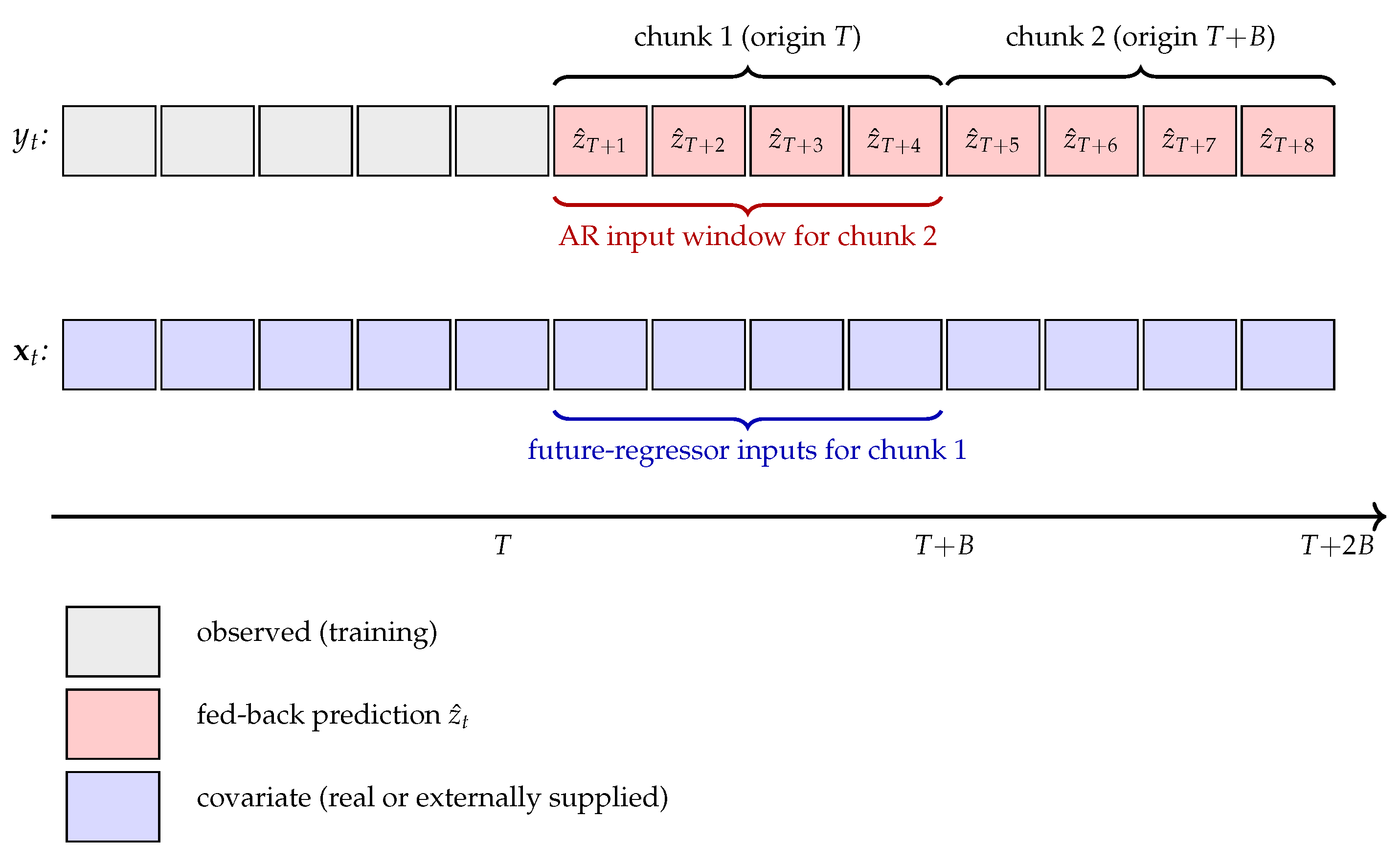
Figure 2.
Continuous forecast against the true latent on the test set. Points are colored by true category; dashed lines mark the true thresholds (on ) and the recovered thresholds (on ). The near-linear association demonstrates that the forecaster recovers the latent ordering.
Figure 2.
Continuous forecast against the true latent on the test set. Points are colored by true category; dashed lines mark the true thresholds (on ) and the recovered thresholds (on ). The near-linear association demonstrates that the forecaster recovers the latent ordering.
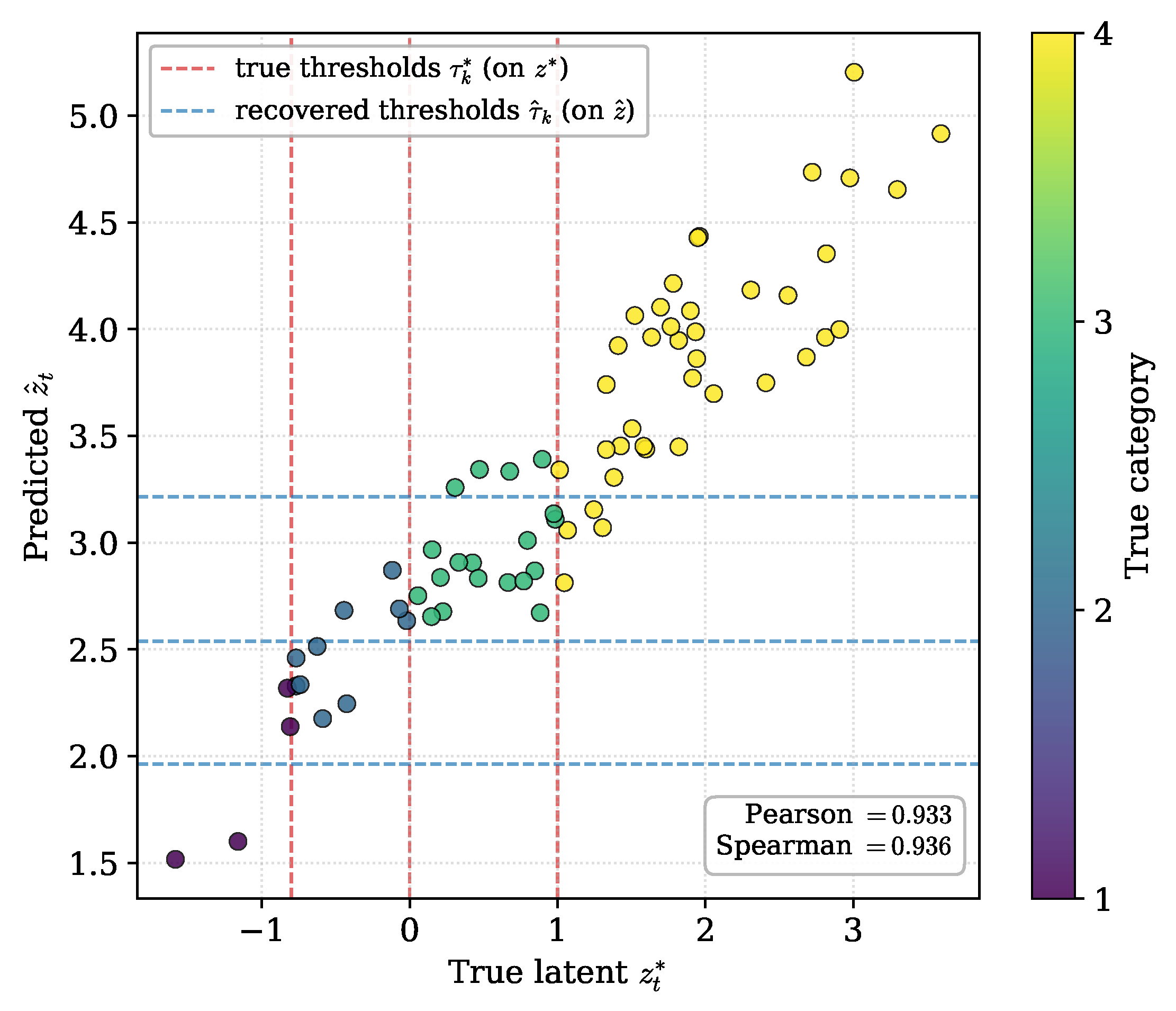
Figure 3.
Fitted components against the true generating components for a representative seed. Trend (centered), daily seasonality, weekly seasonality, and the regressor coefficients. Seasonality and covariate structure are recovered in shape, sign, and ranking; the small trend is only partially recovered. Magnitudes are compressed by the integer-label scale.
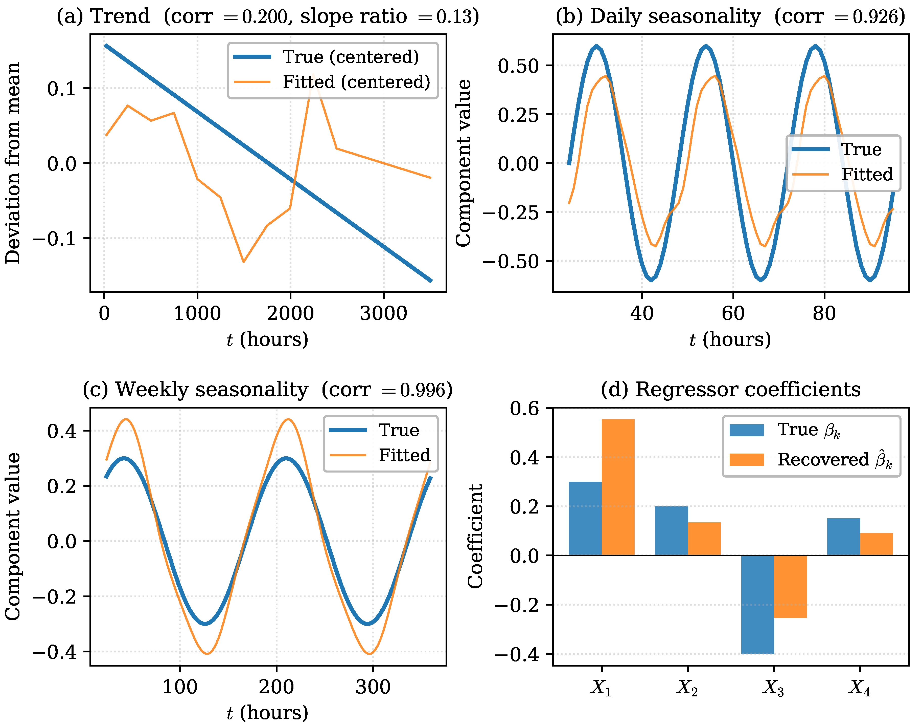
Figure 4.
Recovery of piecewise-linear trends with one, two, and three reversals for a representative seed. Dotted vertical lines mark the true change points. The fitted trend tracks the successive reversals in all three cases, with the correlation declining gradually as the trend becomes more oscillatory.
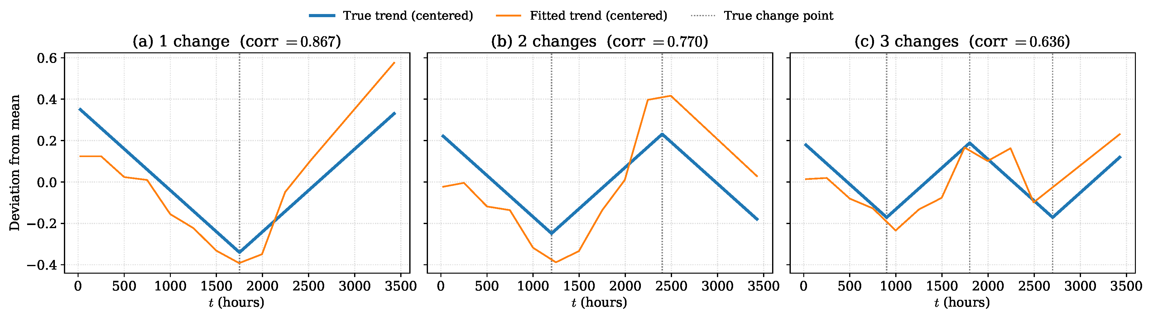
Figure 5.
Quadratic weighted under naive rounding and threshold optimization as a function of the noise level , with the shaded region marking the optimization gain. Error bars are one standard deviation across 20 seeds. Both mappings degrade as noise increases, while the optimization gain remains roughly stable.
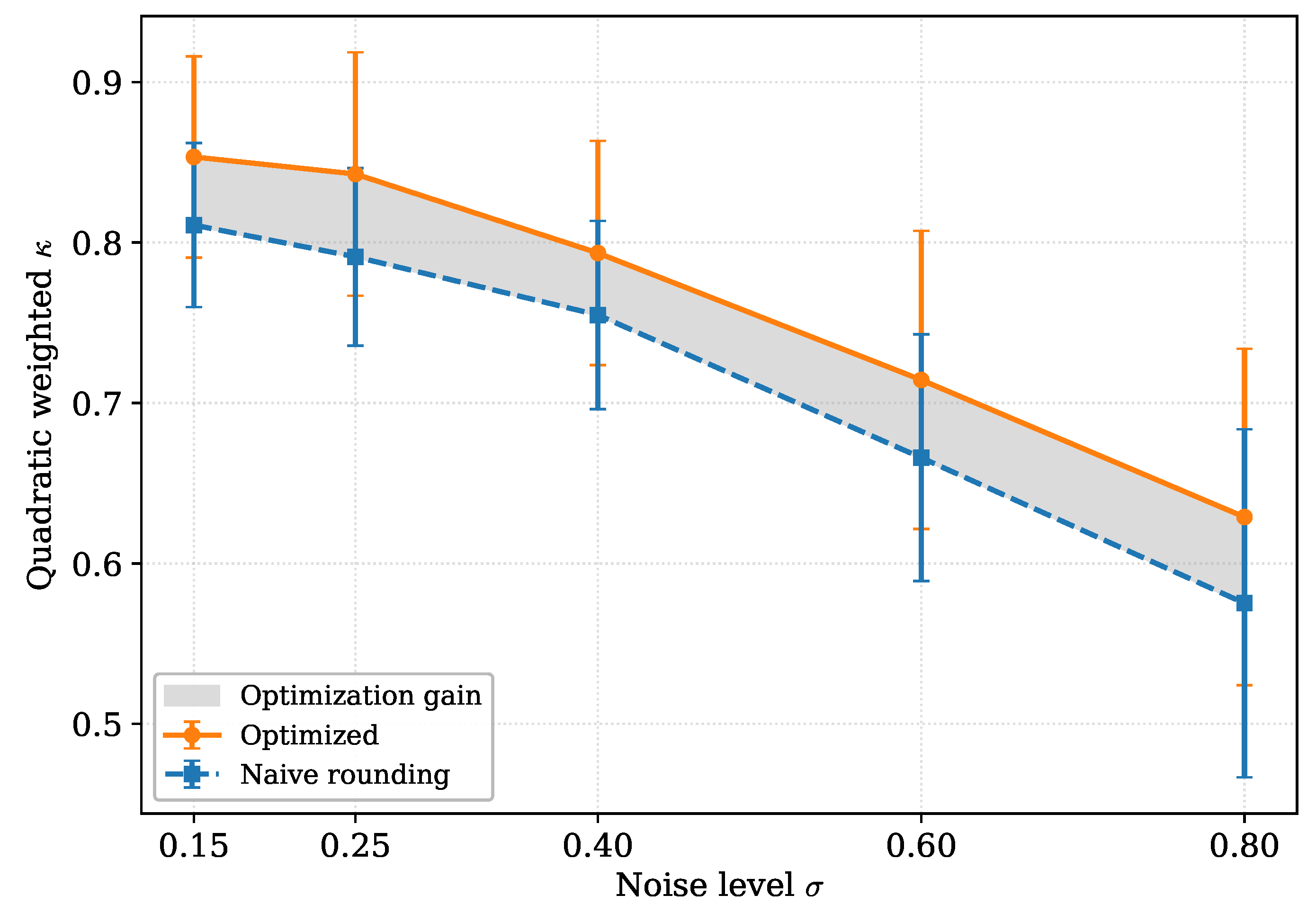
Figure 6.
Two-week windows of (a) Beijing air quality and (b) building load, on the category scale the model observes. Weekends are shaded; the y-axis names each category and gives the band defining it.
Figure 6.
Two-week windows of (a) Beijing air quality and (b) building load, on the category scale the model observes. Weekends are shaded; the y-axis names each category and gives the band defining it.
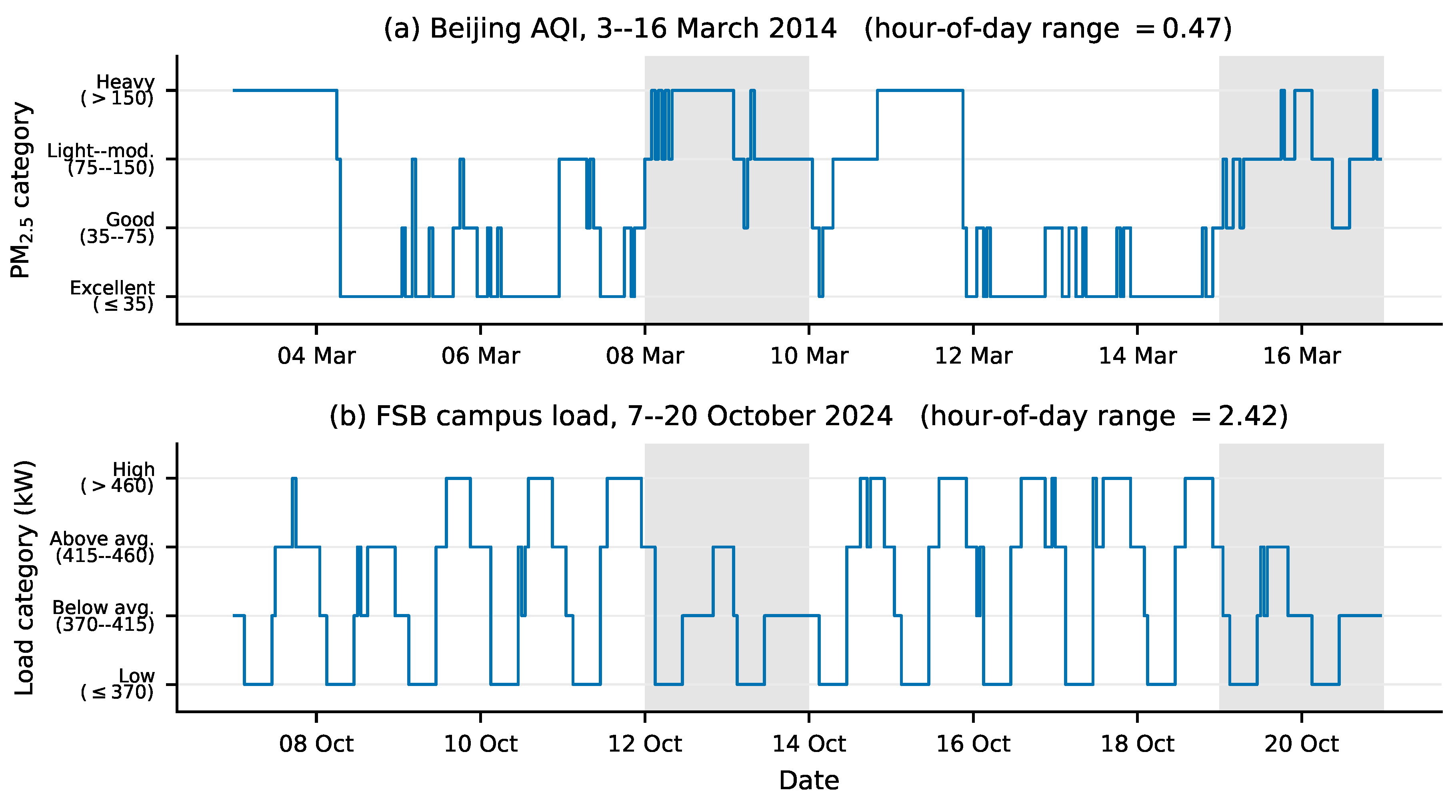
Figure 7.
Quadratic weighted against forecast horizon H for (a) Beijing air quality and (b) electricity load in a Ball State University building, on a common vertical scale from to 1. Both panels show the two-stage method, under optimized thresholds and under naive rounding, against persistence and the two multinomial logistic baselines.
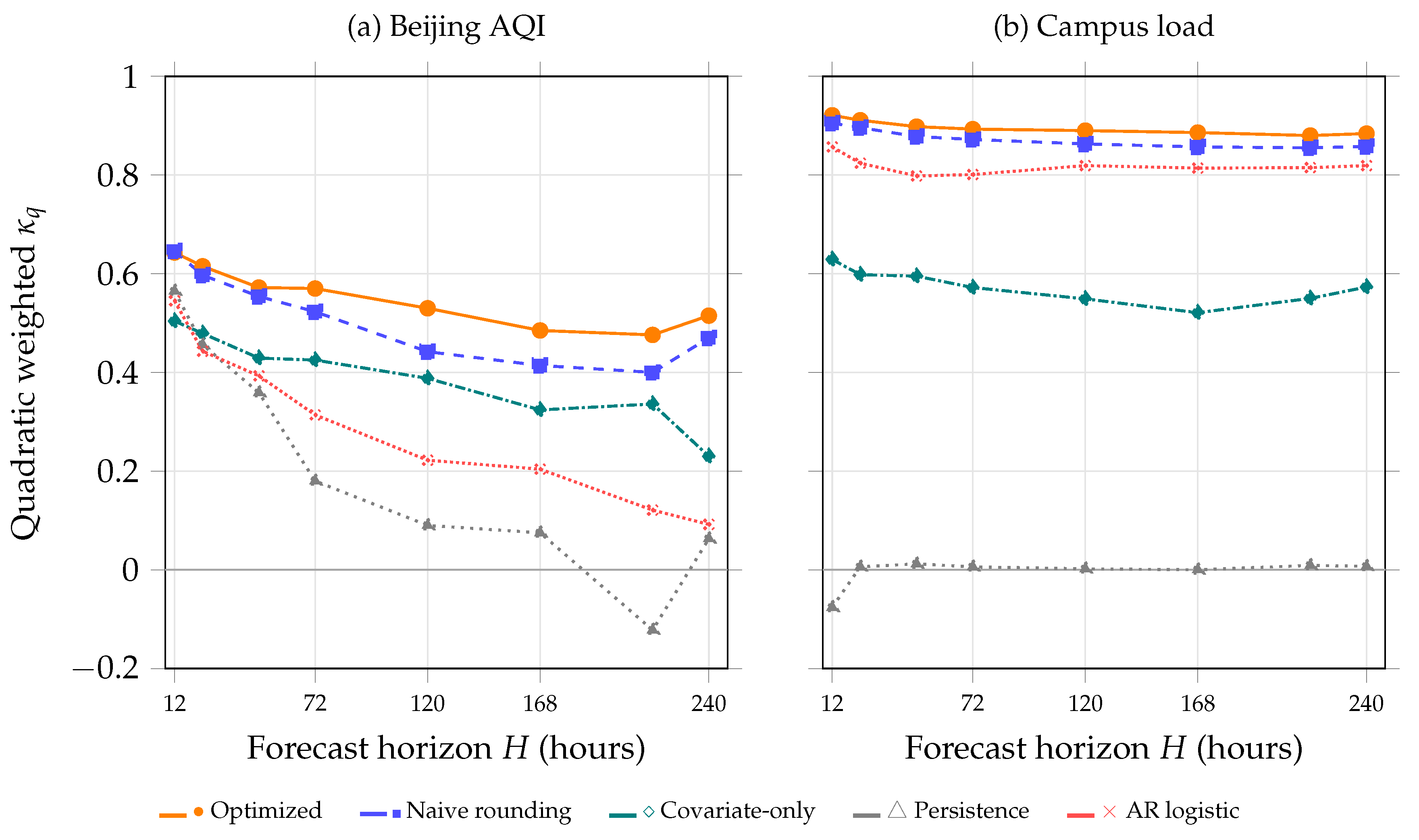
Figure 8.
Fitted NeuralProphet daily and weekly seasonality on the integer-label scale for Beijing air quality (a, c) and Foundational Sciences Building load (b, d). Vertical axes are not shared. Panel titles report the component standard deviation. Campus load is a clock-driven series; Beijing seasonality is present but small relative to the weather contribution in Table 11.
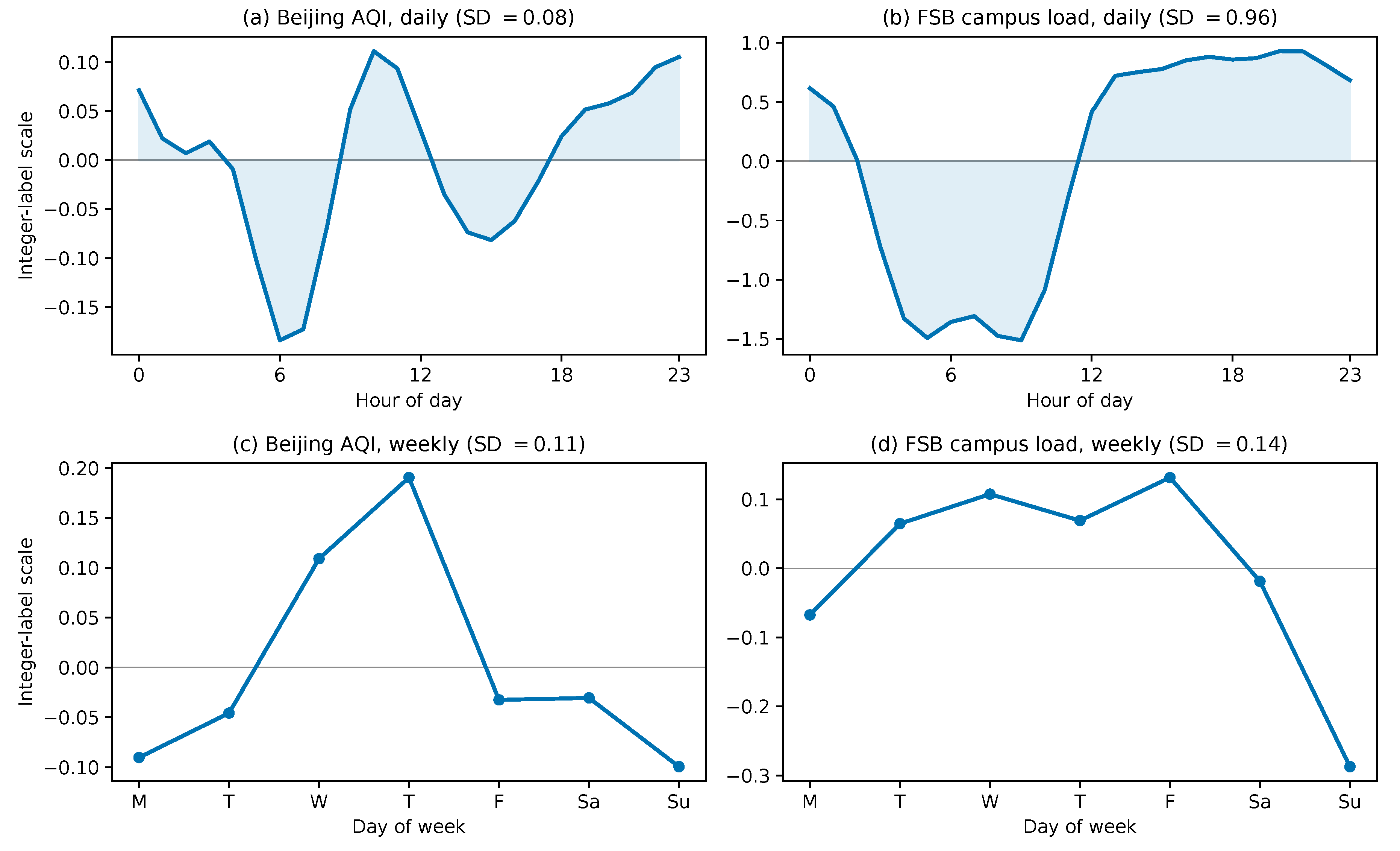
Figure 9.
Per-regressor future-regressor contributions on the integer-label scale for (a) Beijing air quality and (b) Foundational Sciences Building load, ordered within each series by the magnitude of the contribution. Vertical axes are not shared across panels.
Figure 9.
Per-regressor future-regressor contributions on the integer-label scale for (a) Beijing air quality and (b) Foundational Sciences Building load, ordered within each series by the magnitude of the contribution. Vertical axes are not shared across panels.
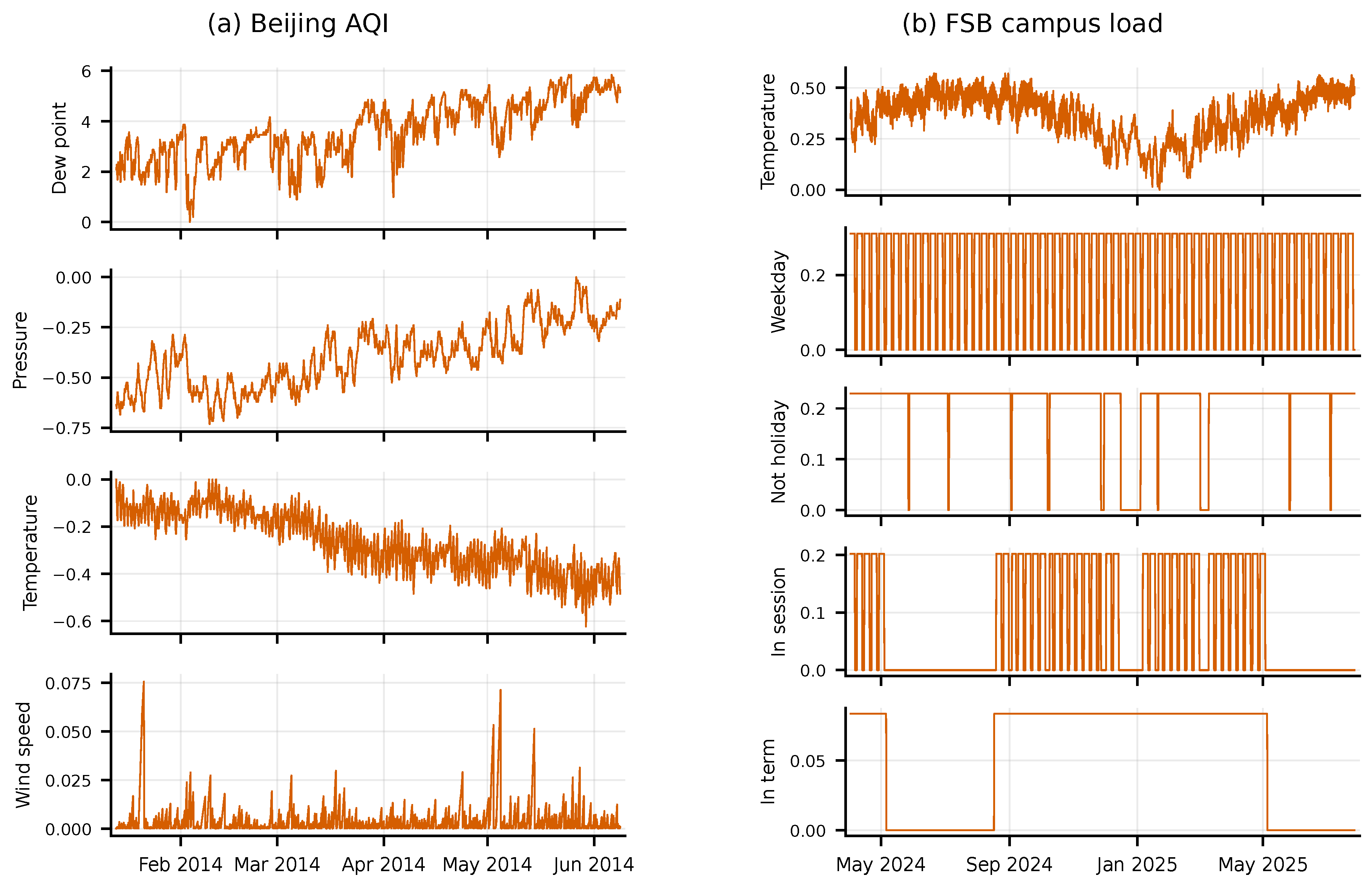
Table 1.
Notation for the forecasting configuration. Values used throughout the experiments are given in Section 4.1.3 and Section 4.2.2.
Table 1.
Notation for the forecasting configuration. Values used throughout the experiments are given in Section 4.1.3 and Section 4.2.2.
| Symbol | Meaning |
|---|---|
| B | Output block width: the number of steps the model emits in a single forward pass (NeuralProphet’s n_forecasts) |
| H | Forecast horizon: the number of steps forecast blind from an origin, covered by chained blocks |
| Number of autoregressive lags of the target | |
| Number of lags of each covariate entering the lagged-regressor component, with | |
| K | Number of ordered categories |
| N | Length of the held-out test block; the horizon spans it, so throughout |
Table 2.
Baseline data-generating parameters for the simulation.
| Component | Parameter | Value |
|---|---|---|
| Length / frequency | n, sampling | 3500, hourly |
| Categories | K | 4 |
| Thresholds | ||
| Trend | ||
| Daily seasonality | amplitude | |
| Weekly seasonality | amplitude | |
| Covariate effects | ||
| Autoregression | ||
| Noise |
Table 3.
True versus recovered regressor coefficients at the reference configuration. All signs are recovered; magnitudes are compressed by discretization onto the integer-label scale, except , which is inflated by absorbing part of the daily cycle it carries.
Table 3.
True versus recovered regressor coefficients at the reference configuration. All signs are recovered; magnitudes are compressed by discretization onto the integer-label scale, except , which is inflated by absorbing part of the daily cycle it carries.
| Covariate | True | Recovered | Sign |
|---|---|---|---|
Table 4.
Threshold optimization versus naive rounding on the simulated test set at the reference configuration, reported as mean ± standard deviation across 40 seeds. Quadratic is the optimization objective; linear is reported for comparison.
Table 4.
Threshold optimization versus naive rounding on the simulated test set at the reference configuration, reported as mean ± standard deviation across 40 seeds. Quadratic is the optimization objective; linear is reported for comparison.
| Metric | Naive rounding | Optimized | Change |
|---|---|---|---|
| Quadratic () | |||
| Linear () | |||
| Exact accuracy | |||
| Within-one accuracy | |||
| MAE |
Table 5.
Threshold optimization under piecewise-linear trends, quadratic weighted as mean ± standard deviation across 40 seeds per condition. Trend shapes correspond to Figure 4; the reference condition uses the single linear trend of Table 2.
| Trend | Naive rounding | Optimized | Change | Improved |
|---|---|---|---|---|
| Reference (linear) | ||||
| One change | ||||
| Two changes | ||||
| Three changes |
Table 6.
Noise sweep at the reference configuration, quadratic weighted and latent recovery as mean ± standard deviation across 20 seeds per level.
Table 6.
Noise sweep at the reference configuration, quadratic weighted and latent recovery as mean ± standard deviation across 20 seeds per level.
| Naive rounding | Optimized | Change | Spearman | |
|---|---|---|---|---|
Table 7.
Summary of the two real datasets.
| Dataset | Domain | Freq. | K | Covariates | Category source |
|---|---|---|---|---|---|
| Beijing AQI | Air quality | hourly | 4 | TEMP, DEWP, PRES, Iws | HJ 633-2012 [1] |
| FSB building load | Energy load | hourly | 4 | temperature, occupancy | discretized load |
Table 8.
Summary at the headline horizon under blind multi-step forecasting, both series. Metrics are pooled by concatenating predictions and observations across non-overlapping origins. We do not report a fold-wise standard deviation because kappa is unstable, and at short horizons sometimes undefined, on folds spanning few categories.
| Beijing AQI | FSB building load | |||
|---|---|---|---|---|
| Method | Acc. | Acc. | ||
| Persistence | ||||
| AR logistic | ||||
| Covariate-only logistic | ||||
| NP + naive rounding | ||||
| NP + threshold optimization | ||||
Table 9.
Beijing horizon degradation, pooled across the non-overlapping origins available at each horizon H (hours). “Gain” is optimized minus naive-rounding ; the last two columns are for the optimized method.
Table 9.
Beijing horizon degradation, pooled across the non-overlapping origins available at each horizon H (hours). “Gain” is optimized minus naive-rounding ; the last two columns are for the optimized method.
| H | Folds | Persist. | Round | Optim. | Gain | Acc. | MAE |
|---|---|---|---|---|---|---|---|
| 12 | 120 | ||||||
| 24 | 60 | ||||||
| 48 | 30 | ||||||
| 72 | 20 | ||||||
| 120 | 12 | ||||||
| 168 | 8 | ||||||
| 216 | 6 | ||||||
| 240 | 6 |
Table 10.
Foundational Sciences Building load, horizon degradation, pooled across fixed origins after hour 2000 (at most 100 origins per horizon). Columns match Table 9.
Table 10.
Foundational Sciences Building load, horizon degradation, pooled across fixed origins after hour 2000 (at most 100 origins per horizon). Columns match Table 9.
| H | Folds | Persist. | Round | Optim. | Gain | Acc. | MAE |
|---|---|---|---|---|---|---|---|
| 12 | 100 | ||||||
| 24 | 100 | ||||||
| 48 | 100 | ||||||
| 72 | 100 | ||||||
| 120 | 79 | ||||||
| 168 | 57 | ||||||
| 216 | 44 | ||||||
| 240 | 39 |
Disclaimer/Publisher’s Note: The statements, opinions and data contained in all publications are solely those of the individual author(s) and contributor(s) and not of MDPI and/or the editor(s). MDPI and/or the editor(s) disclaim responsibility for any injury to people or property resulting from any ideas, methods, instructions or products referred to in the content. |
© 2026 by the authors. Licensee MDPI, Basel, Switzerland. This article is an open access article distributed under the terms and conditions of the Creative Commons Attribution (CC BY) license (http://creativecommons.org/licenses/by/4.0/).
Copyright: This open access article is published under a Creative Commons CC BY 4.0 license, which permit the free download, distribution, and reuse, provided that the author and preprint are cited in any reuse.