

Submitted:
02 October 2026
Posted:
07 October 2026
You are already at the latest version
Abstract
Charging infrastructure for battery electric bus (BEB) fleets must be sized against the timing of demand, not only its magnitude: an accurate per-trip energy estimate cannot on its own establish whether a depot’s chargers, contracted grid connection, and dispatch schedule can recover the fleet’s energy deficit without breaching demand-based tariff thresholds. This is especially consequential in resource-constrained settings, where notified-maximum-demand penalties and steep time-of-use differentials turn a mistimed charging load into a direct commercial liability rather than an operational inconvenience. Yet pre-investment planning tools typically treat vehicle energy consumption, dispatch scheduling, and charging infrastructure as separate problems, so a validated demand estimate rarely translates into a validated depot load profile. This paper presents an operational digital twin that converts the per-trip arrival state-of-charge predicted by a companion rolling stock twin into a depot-level charging load profile for the Golden Arrow Bus Services (GABS) electric fleet at the Arrowgate depot in Cape Town, South Africa. The twin reconstructs each bus’s daily duty chain from scheduling data to determine its available charging window, then simulates session initiation, power draw, and duration against these windows using charging behaviour parametrised from depot Open Charge Point Protocol (OCPP) records, including the smart charging constraints already enforced at the depot. Each bus’s state of charge is carried from one depot visit to the next, so an undercharged departure reappears as a lower arrival rather than disappearing from the model. The simulated load profile is validated against 968 OCPP session records from two periods with different depot hardware, achieving energy-per-session agreement of 4.3 to 7.3 % and load-shape correlation of 0.95 to 0.99, and is evaluated against the depot’s contracted notified maximum demand of 3 000 kVA. Scenario analysis quantifies how the charging schedule, charger rate, and site pool limit shift the load profile relative to this threshold and to time-of-use cost exposure, showing that scheduling charging into off-peak windows without a site-wide limit can raise peak demand above uncontrolled charging and beyond the contracted threshold (3 167 against 1 832 kW), that a site pool limit controls peak demand and monthly cost together, and that a 30 kW per-charger cap leaves buses unable to complete up to 15 % of their trips. By coupling a validated, condition-aware demand layer to depot dispatch and charging logic, this work supports capital-efficient charging infrastructure decisions for transit operators in the Global South, where undersized infrastructure risks service disruption and oversized infrastructure diverts capital from wider electrification.
Keywords:
battery electric bus
; sustainable transport electrification
; digital twin
; charging infrastructure planning
; notified maximum demand
; time-of-use tariff
; depot operations
; sub-Saharan Africa
1. Introduction
The global transition to battery electric bus (BEB) fleets has emerged as one of the most actionable strategies available to municipal transit authorities seeking to decarbonise public transport. Road transport is responsible for approximately 15% of global CO2 emissions, within a transport sector that as a whole accounts for roughly a fifth of energy-related global emissions [1]; public transport represents a comparatively small but growing-priority share of this total, given the scale of fleet electrification programmes now underway in cities worldwide. Unlike a straightforward vehicle replacement, however, BEB adoption introduces a planning requirement that persists even after a fleet’s per-trip energy demand is known: that demand must still be translated into a depot-level charging load profile that the site’s contracted grid connection, chargers, and dispatch schedule can actually deliver [2,3]. This translation step is not incidental to infrastructure sizing; it is the step at which sizing decisions are actually made. A validated estimate of how much energy each bus will need on return from service says nothing, on its own, about whether the depot can recover that energy within the bus’s available charging window, at what rate chargers must draw power to do so, and whether that aggregate draw stays below the site’s contracted demand threshold.
This translation problem is materially harder in resource-constrained grid environments than in the stable-grid contexts in which most electrification planning tools have been developed and validated. In South Africa, transit operators contract a maximum demand threshold under the Notified Maximum Demand (NMD) mechanism, and drawing beyond it carries both financial penalties and grid-stability consequences [4]. Time-of-use (ToU) tariff structures compound this exposure: under the City of Cape Town’s Large User Medium Voltage ToU schedule, energy consumed in weekday peak windows can cost several times the off-peak rate [5]. For a large bus depot, where dozens of buses return from service within a narrow window, and each requires kilowatts of charging power, an uncoordinated or mistimed charging load is not merely an inefficiency to be optimised away later; it is a direct commercial liability the moment it is switched on, and in the worst case a risk to local distribution infrastructure that was never sized for a coincident load of that magnitude. Mischaracterising this load at the pre-investment stage propagates directly into infrastructure decisions that are expensive, and often impractical, to reverse once chargers are installed and a grid connection is contracted: undersized infrastructure or an undersized contracted capacity produces missed departures and service disruption, while oversized infrastructure commits capital that could otherwise fund a wider electrification programme [6].
The individual components of this depot-level planning problem are addressed, to varying degrees, in isolation. Vehicle energy consumption modelling has advanced considerably, with route geometry, ambient temperature, and operating conditions all shown to shift per-trip demand in ways a single fleet-average figure cannot represent [7,8,9]. A companion contribution to this work develops and validates a rolling stock digital twin that predicts this per-trip demand for the same fleet studied here, converting route-geometry and operating-condition features into a predicted arrival state of charge to within 2.95 to 3.46 percentage points depending on route familiarity [10], removing the need to assume a flat consumption rate. What remains open is how that validated per-trip demand is converted into an operational charging plan: which bus charges when, at what power, for how long, and what the resulting depot-level load looks like against the site’s grid and tariff constraints. Charging-infrastructure optimisation studies have addressed parts of this problem, but typically rely on assumed or stochastically generated vehicle arrival patterns rather than empirical operating logs, seeding arrival distributions with Monte Carlo methods where field data are unavailable [11] or sizing infrastructure around a consumption figure that is assumed rather than predicted from the routes actually driven [12]. The one study grounded in the same fleet and depot as this paper was itself seeded with observed arrival state-of-charge values rather than a predictive demand model, treating the link between vehicle operation and charging requirement as an external input rather than a twin-derived output [13].
The digital twin (DT) concept provides the architectural framework within which this depot-level translation problem can be operationalised for pre-investment planning. A DT is a high-fidelity virtual representation of a physical system that can be parametrised from historical operational data and used to evaluate infrastructure configurations in a risk-free environment before capital is committed [14,15]. Applied to depot operations, a DT converts a fleet’s dispatch schedule and predicted per-trip energy demand into a simulated charging load profile, reproducing the aggregate power draw the depot’s chargers and grid connection would actually experience under a given fleet size, charger configuration, and scheduling strategy. Although DT technology has been validated at the scale of hundreds of buses and multiple depots in European metropolitan networks [2], and depot-level load projections have been produced from field data at comparable scale [3], no such operational twin has been developed and validated against independent charging records for a scheduled public transit fleet operating under sub-Saharan African grid and tariff conditions, where the consequences of a mis-sized or mistimed load are structurally more severe than in the stable-grid contexts these frameworks were built for. This study adopts the pre-investment planning mode of the digital twin concept, detailed in Section 2: the twin is parametrised from historical operational data rather than maintaining a live bidirectional connection to the physical asset, which is the operationally appropriate form for infrastructure sizing decisions made before a fleet, or its charging infrastructure, is deployed.
1.1. Contribution
This paper addresses that gap by presenting the development and validation of an operational digital twin that converts predicted per-trip vehicle energy demand into a depot-level charging load profile for the Golden Arrow Bus Services (GABS) electric bus fleet at the Arrowgate depot in Cape Town, South Africa. The twin takes as its input the per-trip arrival state of charge produced by a companion rolling stock digital twin [10], reconstructs each bus’s daily duty chain from GABS scheduling data to determine when it is at the depot and available to charge, and simulates the timing, rate, and duration of each charging session against these windows, carrying each bus’s state of charge from one visit to the next. Charging behaviour, including the smart charging constraints already enforced at Arrowgate, is parametrised from Open Charge Point Protocol (OCPP) records drawn from the depot’s charging station management system. The resulting simulated depot load profile is validated against observed depot charging in OCPP records from two periods, on quantities to which the twin was not tuned, and evaluated against the depot’s contracted notified maximum demand and the City of Cape Town’s time-of-use tariff structure. The principal contributions of this work are: (i) an empirically parametrised operational digital twin that closes the gap between a validated per-trip energy estimate and a validated depot-level charging load, for a BEB fleet operating in a sub-Saharan African context; (ii) a reproducible methodology for reconstructing bus-level charging windows and simulating aggregate charging load directly from duty schedules and OCPP records, requiring no assumed arrival distributions; and (iii) a scenario analysis, on the depot’s real fleet, quantifying how the charging schedule, charger rate, and site pool limit shift the depot’s peak demand and tariff exposure, intended to support charger and grid-connection sizing decisions before capital is committed.
This operational twin is the second layer of a broader digital twin system under development for the Arrowgate depot, built on the rolling stock demand layer described above [10] and intended for future integration with solar photovoltaic and battery energy storage twins currently under development. Sizing decisions for those renewable and storage assets are properties of that full system and fall outside the present paper’s scope. What this paper establishes is that a validated per-trip demand estimate can be reliably translated into a validated depot-level load profile, the step on which charger count, charger rating, and contracted grid capacity decisions directly depend. Because undersizing and oversizing this infrastructure carry different but equally consequential sustainability costs, service disruption and stranded diesel operation on the one hand, wasted capital that could otherwise fund fleet electrification on the other, a validated operational layer is, alongside a validated demand layer, a precondition for capital-efficient, low-risk electrification in resource-constrained transit systems.
2. Literature
This literature review establishes the foundation for an empirical operational digital twin by evaluating the state of the art in charging-infrastructure scheduling, digital-twin deployment for depot operations, and the treatment of resource-constrained grid conditions, before identifying the current research gap.
2.1. Charging Infrastructure Optimisation and Scheduling
Sizing and scheduling charging infrastructure for a BEB fleet is a distinct problem from predicting how much energy that fleet will consume. Even where per-trip demand is well characterised, the depot must still determine which bus charges when, at what rate, and for how long, subject to the constraint that every bus be available for its next scheduled departure. Kunith et al. formulated the joint placement of fast-charging infrastructure and battery-capacity sizing as a capacitated set-covering problem, establishing a foundational framing for cost-effective infrastructure planning at the network level [16]. Building on this direction, An formulates battery-electric bus infrastructure planning explicitly under energy-demand uncertainty [17], while He et al. jointly optimise charging-infrastructure placement, vehicle scheduling, and charging management within a single framework [18]. Mixed-integer linear programming approaches have also been applied directly to depot-level charging schedules; a MILP scheduling strategy calibrated with real operating data from the same fleet and depot studied here reduced the peak demand charge by 17% while keeping total depot demand below 1 MW and ensuring full fleet readiness [13], and hardware-level interventions such as capping individual charger output to keep buses within a constant-current charging phase have been shown to constrain aggregate depot draw within a fixed off-peak window at the same site [13].
A recurring limitation across this body of work is the treatment of vehicle arrival and departure patterns. Many studies rely on assumed or stochastically generated arrival distributions rather than empirical operating logs; Monte Carlo methods are used to seed arrival distributions where field data are unavailable [11], and fleet-electrification cost models size infrastructure around a consumption and arrival pattern that is assumed rather than derived from the routes and duties actually operated [12]. Where real fleet telematics have been incorporated, the resulting scheduling strategies are more operationally credible, but the arrival state of charge is frequently supplied as an external, observed input rather than propagated from a predictive vehicle energy model [13]. This separation between predicted demand and simulated charging behaviour is the gap a companion contribution to this work addresses on the demand side [10], and which the present paper addresses on the operational side.
The consequence of unmanaged versus managed charging at depot scale is well documented. Uncoordinated charging, in which vehicles begin drawing power immediately upon return from service, produces an unevenly distributed load profile with high peaks that is problematic both for the local grid and for equipment dimensioning at the depot [19]. At Arrowgate, buses are connected on return from 17:00 but held until the off-peak window opens at 22:00, and the measured depot load steps up as that window opens; in simulation, 50 buses charging unmanaged at 60 kW reach about 1 MW in the evening return window [13]. Smart charging strategies that stagger session initiation and cap individual charger power have been shown to constrain aggregate depot demand well below what an unmanaged profile would produce, with peak-shaving algorithms developed specifically for large-scale bus depots [19] and smart charging optimisation reducing average peak power demand by 49.8% across a large European metropolitan bus network [2]. What this literature does not generally address is how such scheduling strategies interact with a demand-side twin whose per-trip consumption estimates already vary with route, time of day, and ambient conditions rather than assuming a flat rate; most charging-optimisation studies take fleet energy demand as a fixed or externally supplied parameter, leaving the coupling between a condition-aware demand model and the resulting depot load profile largely unexamined.
2.2. Digital Twins for Depot Operations and Pre-Investment Planning
The digital twin provides the architecture within which vehicle-level demand and depot-level charging behaviour can be coupled into a single planning instrument. A digital twin is a virtual representation of a physical system maintained from operational data, distinguished from a static simulation by its capacity to be parametrised from real measurements and used to evaluate configurations before they are built [14,15]. For pre-investment planning, the relevant mode is a twin parametrised from historical operational data rather than a live bidirectional feed, since it does not control a physical asset in real time but instead allows infrastructure and scheduling scenarios to be tested at model scale before capital is committed.
Such frameworks have been validated at an operationally significant scale. The eflips-X framework modelled Berlin’s bus network against large volumes of real driving data, integrating energy modelling, scheduling, and charging into a single environment [2], and depot-level studies have projected consumption and load for fleets of hundreds of buses using field data [3]. Outside the transit context, coordinated digital twins that couple vehicle charging with other on-site energy assets have demonstrated that treating charging as one component of an integrated, co-optimised system yields materially different outputs than scheduling it in isolation: a four-twin framework spanning photovoltaic generation, stationary storage, electric vehicles, and facility infrastructure reduced operational costs for a waste-collection fleet relative to the industry’s existing procedure [20], and a discrete-event digital twin coupling vehicle charging with production demand and dynamic electricity pricing in a manufacturing context achieved substantial energy cost reductions over uncontrolled and first-come-first-served charging strategies [21]. A comparable digital twin of charging stations for rental EV fleets similarly showed that jointly modelling charging stations and vehicles under predicted mobility patterns supports higher self-sufficiency and lower operating cost than scheduling charging sessions independently of the wider energy system [22].
What these large-scale implementations have in common, however, is that they were developed and validated in stable-grid, temperate-to-cold European operating contexts, or in industrial settings where the marginal cost of unmanaged charging is a matter of energy-cost optimisation rather than a binding grid-capacity or demand-penalty constraint [2,3,20]. Depot-level digital twins explicitly designed to test infrastructure configurations against a hard demand-based penalty threshold, rather than against a continuous cost-minimisation objective alone, remain comparatively rare; the GABS Arrowgate depot studied in this paper is itself one of the few sites where such a threshold has been treated as the primary planning constraint [13], discussed further below. None of the frameworks reviewed here validates their simulated load profile against independently metered charging records from the same site, the validation step this paper undertakes.
2.3. The Empirical-Grounding Gap in a Resource-Constrained Context
The limitation identified above is sharpest in the operating context of this study. South Africa’s Notified Maximum Demand mechanism requires operators to contract a maximum demand threshold in advance, with both financial and grid-stability penalties for exceeding it [4,13], and the City of Cape Town’s time-of-use tariff structure imposes a substantial cost differential between peak and off-peak charging periods [5]. These are not background conditions that a charging schedule can treat as secondary to cost minimisation; they are hard constraints that determine whether an infrastructure configuration is viable at all. Grid capacity itself is also less certain in this context than in the stable-grid settings in which most of the frameworks reviewed above were developed, meaning that a depot-level twin intended for this environment must be validated not only against cost or peak-magnitude criteria but against the specific regulatory and tariff thresholds the operator faces [13].
The work most closely grounded in the same fleet and depot as this study, a charging-optimisation analysis of the GABS Arrowgate depot, addressed exactly this regulatory environment, evaluating scheduling strategies against the depot’s contracted demand threshold [13]. That study, however, was seeded with observed arrival state-of-charge values rather than a predictive vehicle energy model, meaning the charging schedule it evaluated was decoupled from route geometry, ambient conditions, and the other operationally variable drivers of per-trip demand identified in the companion rolling stock twin developed for this fleet [10]. More broadly, no operational digital twin has been developed that both propagates a condition-aware, empirically validated per-trip demand estimate into a depot-level charging simulation, and validates the resulting load profile against independently metered charging records, for a scheduled public transit fleet operating under sub-Saharan African grid and tariff conditions. This paper addresses that gap by coupling the validated demand layer established in [10] to an empirically parametrised charging and dispatch simulation, and by validating the resulting depot load profile against Open Charge Point Protocol records from the same depot.
3. Method
3.1. Depot, Fleet and Tariff Context
The twin models the Golden Arrow Bus Services (GABS) electric bus fleet at the Arrowgate depot, Cape Town, South Africa, over two periods in 2025: 14 to 18 July and 1 to 5 September. The fleet and its charging infrastructure both expanded between the two: 30 buses and 24 dual-connector charger units rated 60 kW each (48 connectors) in July, against 62 buses and 30 units rated 120 kW each (60 connectors) in September, sharing a 1 300 kW site pool that came into force in August 2025 (Section 3.5 and Section 3.6). Each bus carries an eight-pack BYD B12 battery of 229.06 kWh usable capacity (Section 3.4).
Tariff structure.
Arrowgate is billed under the City of Cape Town’s Large User Medium Voltage Time-of-Use tariff, 2025/26, including 15 % VAT [5]. Three daily bands apply on weekdays: peak (07:00 to 09:00 and 18:00 to 21:00), standard (06:00, 09:00 to 17:00, and 21:00), and off-peak (22:00 to 06:00). Energy rates additionally vary by season: 1 June to 31 August is the high-demand season, and 1 September to 31 May the low-demand season, with peak-period energy costing more than double in the high-demand season than in the low-demand season at Arrowgate’s rates (R8.1295 against R3.8405 per kWh). July 2025 therefore falls in the high-demand season and September 2025 in the low-demand season, so the two validation eras differ in tariff cost as well as in hardware. The depot’s own charging schedule blocks charging from 06:00 to 09:00 and from 17:00 to 22:00, a wider window than the current tariff’s peak band strictly requires. These hours match the peak periods of the tariff structure previously in force, and the depot has retained them unchanged to keep operations simple. A contracted notified maximum demand of 3 000 kVA applies, compared in this paper against simulated peak power in kW at unity power factor, with a monthly demand charge of R87.27 per kVA of measured peak and a network capacity charge of R20.09 per kVA of the contracted 3 000 kVA regardless of demand drawn.
Scope.
This paper concerns the depot’s electric bus fleet and its charging infrastructure only. Diesel operations and facility loads other than bus charging are outside its scope. Arrowgate’s solar photovoltaic and battery energy storage system (BESS) were operational throughout the validation periods and contribute to the site load used in one validation comparison (Section 4.1), but modelling either system is outside this paper’s scope, reserved for separate components of the wider digital-twin system (Section 1).
3.2. Two-Layer Architecture
The twin is organised around one separation: a connector is a place to plug in, and a kilowatt is a share of a power budget, and different constraints decide the two. Whether a bus holds a connector depends on connector count, assignment order and dwell timing; how much power it draws depends on the site limit, the charger hardware and the battery. Keeping the two apart is the architectural decision this paper’s central contribution rests on, and Figure 1 shows the resulting pipeline.
Each stage is developed in its own section. Section 3.3 describes dispatch events, the OCPP records used for validation, and the calibrated battery-acceptance model. A dispatch event becomes a session, a record of when a bus becomes eligible to charge, how much energy it needs, and by when, in Section 3.4. The physical layer (Section 3.5) holds one slot per connector and decides, minute by minute, which sessions occupy those slots; it knows nothing about power. The electrical layer (Section 3.6) is a function of the physical layer’s output alone: given the connected set and each session’s unit, it applies four limits, in order of pool share, charger rate, unit ceiling and battery acceptance, and delivers the narrowest. The two eras and populations against which this pipeline is run and validated are defined in Section 3.7, and the verification and validation approach itself is described in Section 3.8.
This separation is not merely organisational. The physical layer determines occupancy from connector counts, assignment order, and dwell timing alone, and would produce the same connected set regardless of how much power the depot could supply; the electrical layer determines power from pool, hardware, and battery limits alone, and would produce the same allocation regardless of which specific buses occupied which connectors. Each layer can therefore be verified and reasoned about independently, and the boundary between them, the connected set and unit assignment passed from one to the other, is the only information that crosses it.
3.3. Inputs and Provenance
The twin draws on four kinds of input: the duty schedule and its predicted per-trip energy, the OCPP charging records used for validation, a calibrated battery-acceptance model, and a fleet roster used to match buses across data sources. The twin performs no scheduling, prediction, or telemetry processing of its own.
Duty schedule and predicted energy.
Each depot visit’s arrival time, dwell window, time-of-use (ToU)-adjusted charging start, and predicted next-trip energy arrive pre-merged in a single dispatch events table, the output of a separate operations and dispatch digital twin that precedes this charging digital twin. That twin merges each trip’s context (route, date, duty, scheduled departure) against the predicted energy from the companion rolling-stock digital twin [10] on a shared trip index, then derives each visit’s dwell window by shifting each bus’s departure times forward by one within same-day duty groups: the dwell window closes at the bus’s next scheduled departure, or, for the last trip of the day, at 06:00 the following morning, the municipality’s off-peak/peak tariff boundary. Where the same bus’s next recorded departure falls before 06:00, the charging twin closes the window at that departure instead, since charging credited after a bus has left would otherwise be carried into its next visit (Section 3.4); this applies to 227 of the 377 overnight visits across both periods. A visit is classified as overnight or midday accordingly, and is flagged as arriving in the depot’s charging-blocked window (06:00 to 09:00 or 17:00 to 22:00); the effective charging start defers to 09:00 or 22:00 exactly when arrival falls inside one of these windows, and equals the arrival time otherwise. This operations layer was itself validated against independently reconstructed ground-truth trips for 4 September 2025 (88 of 105 trips matched; the remainder were excluded upstream by the rolling-stock twin’s own quality filter and are inherited by design): arrival time agreement of minutes, predicted-energy error of kWh, and state-of-charge error of percentage points, the last comfortably inside the -point accuracy the rolling-stock twin reports for itself [10], so this layer does not measurably degrade the demand prediction it propagates. This twin treats the rolling-stock twin’s per-trip prediction as given and propagates it unchanged (Section 3.4). The prediction itself depends on route and operating conditions only, not on the state of charge at which a bus starts its trip, so carrying state of charge between visits requires no change to the upstream twins.
OCPP charging records.
Charging behaviour is parametrised and validated against OCPP session records drawn from the depot’s charging station management system, in two forms. Session-level records (start and end time, initial and final state of charge, total energy, and the connector used) cover 14 to 18 July and 1 to 5 September 2025, giving 286 and 682 charger records respectively. Per-minute telemetry, giving power draw at one-minute resolution, is available only for two single-day extracts within those periods: 16 July and 4 September 2025. The charging management system (CMS) platform exposes per-minute telemetry only session by session, with no bulk per-period export, so building even one day’s extract requires one request per session; the two days reported here were the extent that time allowed. Within that constraint, 16 July and 4 September were chosen at random from the weekdays available inside the validated windows, preferring days that represented normal depot operation. The per-minute records are the only source against which load shape and per-bus power can be validated; the session-level records support only session-count and energy-per-session comparisons.
Battery acceptance.
The charge-acceptance lookup used in Section 3.6 is calibrated from a pool of 32 charging sessions confirmed solo: alone on its connector’s gun for the full session, and, even at the worst moment of depot-wide concurrency during it, its share of the site pool would still have exceeded its own average draw, so the session was never meaningfully constrained by either the unit or the pool clip. Four sessions were confirmed solo directly; 28 further candidates were drawn by stratified sampling across charging-rate bands and checked against the same two conditions. Of the 32, 22 were retained for the constant-current-constant-voltage fit; the remaining 10 were solo but had too few data points in the plateau (40 to 80 % state of charge) or taper () regions to fit reliably. This selection is independent of date and window rather than restricted to a particular period; it draws on the depot’s full available OCPP history rather than only the July and September extracts used for validation elsewhere in this paper. One fitted session is also one of the 43 sessions in the 4 September per-minute validation extract, and is disclosed here for that reason; checked against both the July and September per-minute validation extracts, no other overlap between the calibration pool and either validation window was found.
Fleet roster and arrival timing.
A MAC-address roster maps each bus’s onboard telematics identity to its charging account, and is used to identify which buses are common to both the physical-layer simulation and the metered per-minute records (the “like-for-like” subset used in Section 3.6’s validation). The fleet’s own telematics history also supplies the plug-in delay used in Section 3.5: the median gap between a bus’s physical arrival and the start of its charging session, 5.0 minutes for evening returns and 11.0 minutes for morning returns (the latter reflecting a washbay queue ahead of the charger), computed from 16,315 filtered plug-in events across 133 buses between April and August 2026.
3.4. Session Construction
Each depot visit becomes one charging session: a record holding when the bus becomes eligible to charge, how much energy it needs, and by when it needs it. Sessions are the unit that the physical and electrical layers (Section 3.5 and Section 3.6) operate on; nothing downstream of this step knows about trips, duties or routes.
From duty visit to session.
A depot visit is defined by an arrival and the bus’s next scheduled departure (Section 3.3). Three timestamps carry through into the session: the dwell start, when the bus physically arrives; effective charging start, when the time-of-use schedule first permits charging on or after arrival; and dwell end, the deadline by which the bus must be ready to depart. A session’s connect time is either the effective charging start or the arrival time plus a short plug-in delay, depending on the connect-time rule in effect (Section 3.5); its deadline is always dwell end.
Required energy.
Each visit carries the energy of the trip that brought the bus back to the depot, : on the duty-matched tier, the companion rolling-stock twin’s per-trip prediction [10], propagated unchanged; on the observed-energy tier, the trip’s own observed state-of-charge drop (Section 3.7). kWh is the usable capacity of the fleet’s BYD B12 pack (8 packs of 28.63 kWh). Every session charges towards 100 % state of charge, consistent with the metered charging records, which show a median final state of charge of 100 % and a mean of 96.5 % across the fleet.
State of charge is carried between visits.
A session’s arrival state of charge is not assumed; it is the bus’s departure state of charge from its previous visit, less the trip it has just driven:
where k indexes a bus’s visits in time order, across day boundaries. Because is a simulated outcome, each session’s arrival state of charge is resolved during the simulation, at the moment the session first seeks a connector, by which time its predecessor has departed. A bus that leaves one visit short of full therefore arrives at the next one correspondingly lower, and the energy needed to return it to full, , includes the carried shortfall. Without this, any undercharging would vanish from the model at the next visit instead of accumulating, and a scenario that undercharges would appear to need less energy rather than to fall behind. Three boundary rules apply. A bus’s first visit in a simulated window starts from a departure at 100 %. A gap of more than 36 hours between visits resets the bus to 100 %, on the assumption that it was charged outside the modelled window. An arrival that Equation 1 places below 0 % is floored at 0 % and counted as a stranded trip: one the bus could not have completed on the charge it left with.
Sufficiency.
A session is sufficient if the bus leaves it with enough energy to complete the trip it actually drives next, that is, if its next arrival in Equation 1 is not below zero. Sufficiency is reported as the share of sessions not followed by a stranded trip. Because the test uses the trip the bus actually made rather than a lookup in the duty schedule, it is defined on both tiers (Section 3.7). The energy still owed at the end of a simulated window, each bus’s shortfall below full after its last session, is reported separately as the closing deficit. Every kWh the buses drive is thus accounted for exactly once: delivered, owed at the close, or lost to a stranded trip, an identity checked for every run reported here (Section 3.8).
Coverage.
The July 2025 validation period yields 173 duty-matched sessions across 29 of the fleet’s 30 buses (97 %), and the September 2025 period yields 423 sessions across 62 buses. In July, these split into 114 overnight and 59 midday visits by window type; the mean of 1.52 sessions per bus per day, against an expected 2.00 if every bus completed two duty cycles, reflects visits present in the duty schedule but without a matching charging record, not missing buses.
3.5. Physical Resource Layer
The physical layer holds one slot per connector and decides, minute by minute, which sessions occupy these slots. It knows nothing about power; it releases finished sessions, orders the sessions waiting for a connector, and assigns free slots to them. Its only output is the set of connected sessions and each session’s unit , which Section 3.6 takes as given.
Connectors and Units.
Each of the depot’s charger units exposes two connectors that share one power stage (Section 3.6). A configuration is fixed by its unit count and connectors per unit: 24 units (48 connectors) in the July 2025 validation period, 30 units (60 connectors) in the September 2025 validation period. Every connector is numbered, and connectors and belong to the same unit.
When a session wants a connector.
A session becomes eligible for a connector at its connect time and remains eligible until it is finished. Two connect-time rules are available. Under the first, a session connects only when its charging window opens, so any queueing is pre-empted by the Time-of-Use (ToU) schedule and never appears in the simulation. Under the second, a session connects shortly after the bus physically arrives, and the charging-allowed schedule in Section 3.6 handles any blocking, so a bus can arrive, occupy a connector, and wait unpowered until charging is allowed. All results reported here use the second rule. The plug-in delay between physical arrival and connection is a declared parameter, not fitted: 5.0 minutes for evening returns and 11.0 minutes for morning returns, drawn from the median of 16,315 filtered plug-in events across 133 buses between April and August 2026 (observed ranges 5.3 to 6.5 and 9.4 to 12.1 minutes respectively); the longer midday figure reflects a washbay queue ahead of the charger. A session stops wanting a connector at its deadline, the scheduled time of its next departure, or, for a visit with no further departure that day, at 06:00 the following morning or the bus’s next recorded departure if that is earlier (Section 3.3).
When a session releases its connector.
At Arrowgate, a bus coming off duty plugs in and charges until either it is fully charged or it is due to depart, whichever comes first; if it finishes charging early, it remains connected, drawing no further power, until its next scheduled departure. The twin reproduces this: a session’s connector is released only at its deadline, never earlier, so a bus that finishes charging early continues to occupy, but not draw from, its connector until it departs. A departure that is a quick top-up, a service run, or otherwise unscheduled is outside the twin’s scope, which works from the published duty schedule. A released connector is unavailable for a short changeover of 5 minutes before it can take another session, representing physical reconnection time.
Assigning free connectors.
Sessions waiting for a connector are served in order of connect time, first-come-first-served, and are matched to free connectors in one of two orders. Pack assignment fills connectors by index, so a unit’s second connector is only used once its first is occupied, matching the order in which drivers park at Arrowgate: charger 1’s first connector, then its second, then charger 2’s first connector, and so on. This concentrates sessions on as few units as possible and is the assignment used throughout this paper. Spread assignment instead ranks free connectors by how loaded their unit will be once the current queue is served, favouring empty units over one that already has a session; it was evaluated as an alternative and is not used in the results reported here. Pack assignment is what makes the unit ceiling in Section 3.6 a live constraint: a session assigned to a unit’s second connector shares that unit’s rating with whichever session already occupies the first.
Connection rate.
The twin exposes an optional cap on how many buses can be physically connected per hour, intended for depots where a shunter drives and plugs in every returning bus. It is not used in any scenario reported here: at Arrowgate, an in-service bus is driven and plugged in by its own driver directly from duty, by way of the washbay when needed, with no separate handoff step for the fleet the twin models. Shunters move and connect buses only when they arrive from the workshop, a category outside the scheduled duty chain from which this twin’s sessions are built. The arrival-to-plug-in gap that does occur in practice is instead represented by the plug-in delay described above.
What the physical layer does not do.
It does not compute power, does not know a connector’s rating, and does not decide which session should be prioritised beyond first-come-first-served ordering. If more sessions want connectors than are free, the excess is counted as queued rather than powered at a reduced rate; no scenario reported in this paper produces a non-zero queue, so queueing is not a binding constraint in the results but remains available should a smaller fleet of units be scenario-tested.
3.6. Electrical Allocation Layer
The physical layer (Section 3.5) delivers, for every simulated minute t, the set of sessions that hold a connector and the charger unit that each session i occupies. The electrical layer is a function of that set alone; it converts it into a power draw for each session and never moves a session between connectors. The separation is deliberate. A connector is a place to plug in, whereas a kilowatt is a share of a budget, and the two are limited by different equipment.
Four limits are evaluated for every session in every minute, in the order of pool share, charger rate, unit ceiling and battery acceptance, and the narrowest one sets the power. In the configurations reported here, the charger-rate limit is inactive, so the pool share, the unit ceiling and battery acceptance do the work. Let be the number of connected sessions, the number of those that still need energy, and the number of connectors occupied on unit u. The set point is
with
and the power actually delivered is
where is the one-minute time step. The first three terms are operator and hardware limits, and the fourth is a property of the electric bus’s battery management system (BMS), which is why the battery clip is applied last.
Pool share.
is the site limit set by the depot’s dynamic load balancing (DLB) profile, which holds a maximum load and a time-of-day schedule and is applied through the operator’s charge management system [23]. It is zero during windows when charging is blocked. The profile uses the weighted-average strategy, which divides the site limit in proportion to the rated power of the occupied connectors [23]. All Arrowgate connectors share one rating, so the division becomes equal. The denominator in Equation 3 counts a full bus that keeps its connector at reduced weight. The factor is the fraction of that unused headroom which the load balancer hands to the buses still charging: gives full buses a whole share, and hands their headroom back entirely.
Charger rate.
is a single value per hour that applies identically to every connector; no individual connector is assigned its own rate. It represents a uniform charger-side output cap of the kind examined at this depot [13] and is available in the twin as a scenario control. Arrowgate applies no such cap separate from the unit rating: the effective 30 kW per bus reported at this depot in 2025 [13] is the unit limit shared between the unit’s two connectors, and the site pool limit came into force only in August 2025. None of the scenarios reported here uses it independently of the unit rating, so equals U, the unit clip always reaches the same value first, and the rate clip never decides the outcome (Figure 2). It remains in Equation 2 so that one expression covers every lever the twin exposes.
Unit ceiling.
A dual-connector unit shares one power stage, and the manufacturer specifies a maximum combined output equal to the unit’s rated power [24]. All Arrowgate chargers are the same make, model and configuration, so the two connectors on a unit carry equal rated power and, under the weighted-average allocation described above, split the unit ceiling equally. The July 2025 units were rated at kW, giving 30 kW to each of two simultaneous sessions, consistent with the tight clustering of per-bus power around 27 to 30 kW observed in the per-minute July telemetry (Section 3.8). The September 2025 units are rated at kW, giving 60 kW to each of two sessions. This is the only clip through which the physical layer influences the electrical layer, since comes from connector occupancy. A held-full bus is counted in , so the split within a unit is static and equal.
Battery acceptance.
The function f is a lookup table over the set point (20 to 120 kW) and state of charge. It is generated from a constant-current constant-voltage kernel [25] calibrated to the 229 kWh BYD pack. Acceptance is capped at about 107 kW at the charger, and the constant-current phase ends at a rate-dependent onset (with s in kW, valid for 70 to 108 kW), after which power decays exponentially with per percentage point. Below 70 kW the constant-current phase is assumed flat. The onset and decay were fitted on 22 unconstrained (solo) sessions selected from 32 candidates, spanning 71 to 108 kW. The onset-rate line is fitted through the median onset of three observed rate levels rather than through all 22 raw points, since 18 of the 22 sessions cluster at the charger’s current ceiling and would otherwise dominate an unweighted fit; on the same 22 sessions this gives a mean absolute onset error of 1.18 percentage points of state of charge, against 3.12 points for a single fixed onset. One session fits 8.2 points below the line despite being the best-sampled session in the pool, which can be attributed tentatively to per-vehicle battery-management variation rather than to charge rate, since the current ceiling group shows a comparable spread (83.2 to 93.4 %) at an essentially constant rate. Below 70 kW the table is not fitted; it assumes flat constant-current charging to 99 % state of charge based on a single controlled session at approximately 30 kW, extended down to a floor of 20 kW below which the model declines to estimate. Acceptance depends on state of charge and rate only; pack temperature is not modelled [26].
Attribution of the binding clip.
For interpretation only, each drawing bus-minute is credited to the clip that set its power. When two clips tie, the credit follows the order: pool, rate, unit. A minute is credited to the battery when delivered power falls more than 0.5 kW below the set point, and to the final-minute clamp when the energy still required limits the draw. This bookkeeping does not alter any result.
The calibrated parameter .
is the only fitted allocation parameter. It was calibrated to the measured overnight peak of the buses common to the simulation and the metered data on 4 September 2025 (569.8 kW across 23 like-for-like buses). Values of , , , and 1 gave simulated peaks of 505.6, 535.3, 574.7, 645.5 and 789.3 kW, and was adopted. Per-minute metered data exist only for that night, so is calibrated on it and not validated by it. The validation targets in Section 3.8 are scale-independent quantities to which was not tuned. Every scenario that depends on reports its range over (Table 1). The value moves the peak demand by about 7 % and the attribution between the pool and the unit clips, but not the delivered energy: with state of charge carried between visits (Section 3.4), every configuration in Table 1 delivers the full 40 632 kWh the fleet drove. Pool and unit together set 96 to 98 % of drawing bus-minutes at every value, and battery acceptance is at most 3.4 %.
Simplifications.
Four simplifications are deliberate. First, the twin divides the power of a unit equally between its occupied connectors, whereas the hardware appears to release power to the remaining bus. In the per-minute records of 4 September, six events on five units show the surviving bus rising from 20.8 to 49.2 kW before its partner finished from 44.1 to 90.7 kW within 15 minutes after, a mean rise of 29 kW, so the static split is conservative. A sensitivity run that instead divides unit power only across sessions still drawing (rather than every occupied connector) leaves the reported peak and total energy for the September configuration unchanged (1 237.1 kW and 40.6 MWh under both), because the unit ceiling binds mainly in the early afternoon (13:00 to 16:00), a window that never sets the depot’s overnight, pool-bound peak, and because this configuration already delivers every kWh the fleet requires under the static split, so faster afternoon delivery does not increase the total. Within that afternoon window the static split is conservative on a finer measure: the unit clip’s share of drawing bus-minutes falls from 66.5 to 36.3 %, the battery-acceptance clip’s share rises from 6.2 to 19.3 % as freed capacity reaches individual buses’ acceptance ceiling, and mean delivered power rises from 62.2 to 67.8 kW. The static split is therefore conservative for individual buses’ charging speed in the afternoon, but does not affect the peak-demand or total-energy results reported in Section 4. Second, the roughly 4 % conversion loss between the charger and the pack is not modelled; the manufacturer’s peak efficiency is at least 96 % [24]. Third, no charger failure mode is represented. Fourth, and by design, the allocation rules are fixed inputs: the twin evaluates a configuration and does not search for a better one.
3.7. Scenario Definitions
Two validation eras.
Results are reported against two periods with different depot hardware (Section 3.5 and Section 3.6): 14 to 18 July 2025, with 24 charger units, 60 kW per unit and no site pool limit, and 1 to 5 September 2025, with 30 units, 120 kW per unit and a 1 300 kW site pool. Each is treated separately throughout; no result combines data across the two.
Two visit populations.
Within each era, sessions can be built from either of two sources, referred to as tiers. The duty-matched tier is built from the published duty schedule and the companion rolling-stock twin’s predicted per-trip energy (Section 3.3). The observed-energy tier is instead built directly from GPS-based trip detection, taking each visit’s required energy from its observed state-of-charge drop rather than a prediction, and classifying window type by dwell duration rather than arrival hour alone.
The two disagree substantially on coverage. Traced to source, the duty-matched tier under-covers because the duty-schedule export records an EV fleet number reliably for morning duties (93.9 % matched) but not for afternoon ones (74.5 %): a bus’s morning duty may carry its own fleet number while its afternoon duty on the same vehicle appears under a diesel placeholder. This is a limitation of the schedule export, not of the twin’s matching logic, and does not affect the observed-energy tier, which needs no duty match at all. Against the charger records taken as the reference count, duty-matched coverage is 60 % (173 of 286 sessions) in July and 62 % (423 of 682) in September; observed-energy coverage is 76 % (216 of 286) and 74 % (506 of 682) respectively. Table 2 summarises both tiers for both eras.
Validation against per-minute and session-level metered records (Section 3.8) uses the observed-energy tier, since it is closer to a complete count of what the depot actually did and its required-energy figures are themselves measured rather than predicted. The use-case scenarios below are reported on the observed-energy tier for the same reason, and repeated on the duty-matched tier as a cross-check. With state of charge carried between visits, the duty-matched tier’s missing afternoon duties have a directional effect: a missing trip is never subtracted from the bus’s battery, and its time on the road appears as additional dwell, so that tier makes buses look better charged than they were. The sufficiency test (Section 3.4) is defined on both tiers. The duty-matched tier remains the one through which the companion twin’s predicted demand enters the simulation, and agreement between the two tiers on the scenario comparisons is what the cross-check tests.
Use-case scenarios.
Seven scenarios are defined on the September hardware, run on the observed-energy tier with the duty-matched tier as a cross-check, varying only the charging schedule, the per-unit charger rate, and the site pool limit; every other feature (dual-connector sharing, hold-from-arrival, hold-until-departure, overshoot clamping, and headroom redistribution) is held fixed across all seven, so that any difference between them is attributable to the varied lever alone. Uncontrolled charging removes the time-of-use schedule entirely, so every session may draw power as soon as it connects; schedule control only restores the time-of-use blocking with no site limit, which is the depot’s existing practice of holding buses until the off-peak window opens, applied to the September hardware; the schedule control + pool cases add a site limit of 1 300 or 1 000 kW; and schedule control + 30 kW instead caps every charger at 30 kW with no site limit. Table 3 lists the seven configurations; their simulated outcomes are reported in Section 4.
3.8. Verification and Validation Design
Verification and validation are treated as distinct exercises [27]: verification asks whether the implementation does what the conceptual model specifies, independent of any comparison to the real depot; validation asks whether the model’s behaviour agrees with observed depot behaviour, at whatever level of agreement is appropriate to how the model will be used.
Verification.
The physical and electrical layers (Section 3.5 and Section 3.6) are built as an ordered sequence of features, each added on top of the last and re-run against the full population, so that every feature’s individual effect on peak demand, delivered energy, and sufficiency is visible before the next is added. Adding the binding-clip attribution used in Section 3.6’s figure (Figure 2) is verified the same way: introducing it does not alter the simulation’s numerical results, since it only labels a value already computed rather than changing how that value is computed, confirmed by re-running the full feature sequence before and after and comparing every reported figure by hand. Carrying state of charge between visits (Section 3.4) was added as a switchable feature and verified by two automated checks. With the feature switched off, the twin reproduces the preceding version’s energy, peak demand and sufficiency exactly for all seven use-case scenarios. With it switched on, the energy identity of Section 3.4 closes to 0 kWh for every run reported in this paper, with one explained exception: the July validation run, whose configuration leaves the final-minute overshoot clamp off, delivers 66.1 kWh past 100 % state of charge over five days, which the identity correctly attributes.
Validation design principle.
The use-case scenarios (Section 3.7) are run on populations, hardware configurations, and headroom-redistribution settings that differ from any period for which per-minute metered data exists, so the twin cannot be validated by reproducing one specific depot-wide total. Instead, validation targets scale-independent quantities: energy per session, per-bus charging power, and the temporal shape of depot load. These do not depend on how many buses were present on a given day, and so remain meaningful comparisons even though no scenario reported in Section 4 replicates a validated day’s population or configuration exactly. Total delivered energy and absolute peak demand are reported throughout the paper as conditional outputs of a given scenario, never as validation targets in their own right.
Why two eras, not one.
July and September validate different parts of the mechanism, and neither can substitute for the other. July’s hardware has no site pool, so the pool-share clip (Section 3.6), the electrical layer’s central mechanism and its one calibrated parameter , is never exercised that period: no site limit applies throughout. July instead validates the parts of the mechanism that do not depend on the pool: connector assignment, unit sharing, battery acceptance, and overall energy accounting, across five days and 286 charger records. September is the only period with a site pool in force, and is therefore the only period against which the pool-share clip, and , can be validated at all; its per-minute telemetry, however, covers a single night rather than July’s full window. The two eras are reported separately because they are testing different things, not because one supersedes the other.
July 2025.
Two comparisons are made, at two granularities. Across the full five-day window (14 to 18 July), simulated energy per session on the observed-energy tier (Section 3.7) is 94.22 kWh against 90.15 kWh measured across 286 Autel charger records, a 4.5 % gap, and the load shape correlates at 0.977 across the five days. For the single day with per-minute telemetry (16 July), energy per session is 97.9 kWh simulated against 93.9 kWh measured, the load shape correlates at 0.947, and overnight power per connected bus (22:00 to 23:59) is 30.0 kW simulated (pack assignment) against 27.5 kW measured, with a spread-assignment alternative (Section 3.5) instead giving 60.0 kW, evaluated but not used in any reported result. The corresponding figures for this period are presented in Section 4.
September 2025.
On the like-for-like subset of 23 buses common to the simulation and the 4 September per-minute record, the fully-featured configuration (dual-connector sharing, hold-from-arrival, hold-until-departure, overshoot clamping, and headroom redistribution; Section 3.6) gives a load-shape correlation of 0.953 and a mean absolute difference of 0.91 kW per visit against the observed-energy tier, with energy per session of 112.8 kWh measured against 104.6 kWh simulated. The same comparison on the duty-matched tier is weaker (correlation 0.894, mean absolute difference 1.42 kW per visit, 102.9 kWh simulated), consistent with the observed-energy tier’s closer match to actual depot behaviour noted above; the observed-energy figures are the ones reported as this era’s validation result.
The measured overnight peak on this same 23-bus subset (569.8 kW) is not a validation target: it is the figure to which was calibrated (Section 3.6), and comparing the simulation’s output to it after fitting would be circular. As a check that is not circular, a full-population reconstruction using each bus’s real (rather than GPS-derived) arrival time, initial SoC, and required energy for 4 September, still with fixed at its calibrated value, gives a correlation of 0.987 and a mean absolute difference of 0.568 kW per visit against 0.972 and 0.850 kW per visit at ; this improvement is evidence that better represents depot behaviour on quantities it was not fitted to, though it remains a same-day check and does not substitute for validation on an independent night (Section 3.3). The corresponding figures for this period are presented in Section 4.
What is not independently validated.
Three limitations follow directly from the data available (Section 3.3). First, is calibrated to a single night’s overnight peak and not tested against a held-out night, since per-minute telemetry exists for only one day per era; its sensitivity to that choice is instead reported as a range (Table 1). Second, the static equal split of a shared unit’s power (Section 3.6) is evaluated only against six give-back events on 4 September, not a full validation set. Third, one session used to calibrate the battery-acceptance lookup also appears in the 4 September per-minute validation extract (Section 3.3); given the fitted lookup draws on 22 sessions and the extract on 43, this is judged to have negligible effect on the reported comparison, but it is disclosed rather than corrected for.
4. Results
4.1. July 2025 Validation
Three scale-independent claims (Section 3.8) are tested against the charger records for 14 to 18 July 2025, on the observed-energy tier with pack assignment and hold-from-arrival (Section 3.7). Figure 3 presents all three together.
Energy per session.
Across the five days, measured energy per session is 90.15 kWh against 25 781.9 kWh delivered over 286 sessions; simulated energy per session is 94.22 kWh over 216 sessions, an agreement of 4.5 %. Nineteen measured sessions, 0.6 % of total measured energy, deliver under 5 kWh, interrupted plug-ins and top-ups the twin cannot produce since it has no session failure mode (Section 3.6); excluding them raises the measured mean to 96.42 kWh and narrows the gap to 2.3 %, with the simulated value then below the measured one. The full set, including these sessions, is the figure reported.
Power per bus.
Median overnight power per connected bus is 27.5 kW measured against 30.0 kW simulated under pack assignment, and 60.0 kW under spread assignment: pack matches measured behaviour, and spread would draw roughly double. This is corroborated directly, independent of the power comparison itself; at the measured overnight peak minute, 12 of the 18 active charger units had both connectors occupied, physical confirmation that units fill front-to-back as pack assignment models, rather than sessions spreading across more units than necessary.
Load shape.
For 16 July, the one day with per-minute telemetry, measured and simulated load shapes correlate at 0.947 (mean absolute difference 1.05 kW per visit), and session coverage for that day is 80 % (43 of 54 Autel sessions). Direct per-minute charger telemetry, the basis for every other claim in this section, was pulled for this single day only; for the full five-day window, charging load is instead estimated from an independent reconstruction of total site load, combining grid import, solar generation, and battery energy storage system (BESS) discharge into a single site-level consumption series (Figure 4). This reconstruction correlates with the simulated load shape at 0.977 (mean absolute difference 0.16 kW per session, 286 measured against 216 simulated sessions); isolating the charging-specific component of this total requires subtracting the depot’s non-charging base load, interpolated across the hours when charging is blocked, and the resulting reconstructed five-day charging total agrees with the sum of the charging stations’ own per-session records to within 2.8 %, an independent check on the reconstruction method itself, not a fitted result.
4.2. September 2025 Validation
September’s hardware includes an active site pool (Section 3.1). Both comparisons below use the 23 buses common to the simulation and the 4 September per-minute charger record, the fully-featured configuration (dual-connector sharing, hold-from-arrival, hold-until-departure, overshoot clamping, and headroom redistribution; Section 3.6).
Tier choice.
The duty-matched tier takes each visit’s energy requirement from the companion twin’s prediction, whereas the observed-energy tier derives it from the visit’s own observed state-of-charge drop (Section 3.7). On the 23-bus subset (Figure 5), the observed-energy tier agrees better with the measured load shape: correlation rises from 0.894 (duty-matched) to 0.953, and the mean absolute difference falls from 1.42 to 0.91 kW per visit. It does not close the gap in energy per session. Measured energy per session is 112.8 kWh, against 102.9 kWh simulated on the duty-matched tier and 104.6 kWh on the observed-energy tier, an agreement of 7.3 % for the tier reported. The simulated value sits below the measured one, opposite in sign to July’s full-set comparison (Section 4.1) but the same sign as July once its 19 sub-5 kWh sessions are excluded (2.3 % below). One candidate contributor is the charger-to-pack conversion loss of roughly 4 %, which the twin does not model (Section 3.6): measured energy is recorded at the charger, whereas the requirement is derived from the change in battery state of charge. This has not been isolated, and the gap is reported as found.
Headroom redistribution, on an independent day.
The redistribution fraction (Section 3.6) was calibrated to the measured overnight peak on this same 4 September subset, so that comparison cannot itself validate . As an independent check, on quantities was not fitted to, the 4 September simulation was re-run with each of the 23 buses’ arrival time and initial state of charge, taken from the charger records, substituted for their GPS-derived equivalents, with each visit’s dwell deadline shifted to match the corrected arrival time. Under this ground-truth arrival configuration, load-shape correlation rises from 0.972 at to 0.987 at , and mean absolute difference falls from 0.850 to 0.568 kW per visit. Both directions of change are consistent with improving, rather than merely reproducing, the fit to depot behaviour on this independent day, though it remains a same-day check and does not substitute for validation against a held-out night (Section 3.8).
4.3. Use-Case Scenarios
Seven scenarios (Section 3.7) isolate the effect of the time-of-use schedule, the per-unit charger rate, and the site pool limit on the September hardware over 5 weekdays. Table 4 and Figure 6 report them on the observed-energy tier (506 visits, 62 buses); Table 5 and Figure 7 repeat them on the duty-matched tier (423 visits) as a cross-check. Every scenario shares the same physical and electrical-layer configuration (Section 3.6) except the schedule, charger rate, and pool limit varied here, so any difference between scenarios is attributable to that lever alone. The two tiers rank the seven scenarios in exactly the same order on peak demand. Absolute values are higher on the observed-energy tier, which holds about 20 % more visits.
Scenarios that keep up need the same energy.
Scenarios 1, 2a, 3 and 4a deliver exactly the same energy, 49 492 kWh over the five days, which is the energy the buses drove. The levers change when and how fast that energy is delivered, not how much of it is needed. Where a scenario delivers less, the difference is energy the fleet still owes or trips it could not complete, not a saving.
Scheduling alone can increase peak demand.
Moving all charging into the off-peak and standard tariff windows, with no pool limit (scenario 3), produces a higher peak than uncontrolled charging (scenario 1): 3 166.9 kW against 1 832.2 kW, a 73 % increase that takes the depot above its contracted 3 000 kVA. This follows directly from the mechanism in Section 3.6: restricting when sessions may draw power without also restricting how much they may draw concentrates the same total energy into a narrower window, and every session still competing for that window draws at its full charger rate simultaneously. The duty-matched cross-check shows the same effect at a lower level (2 520 against 1 500 kW, a 68 % increase), which stays below the contracted threshold; whether scheduling alone breaches it therefore depends on counting the depot’s visits fully. Scheduling still reduces the monthly bill, R821 208 against R876 385, but only because the shifted energy falls in cheaper tariff periods, not because it moderates the load’s magnitude; it is the pool limit, not the schedule, that does that.
The pool limit is what controls peak demand and cost together.
Adding a 1 300 kW site pool to the schedule (scenario 4a) holds peak demand at the limit, 1 300.0 kW against 3 166.9 kW, and reduces the monthly bill from R821 208 to R657 866, a saving of R163 342 per month, almost entirely from the demand charge component, while every bus still completes every trip. A tighter 1 000 kW pool (scenario 4b) reduces peak further, to exactly its own limit, and lowers the bill to R629 668, but leaves one bus unable to complete one trip in the week (sufficiency 99.80 %) on the observed-energy tier, and none on the duty-matched tier: at 1 000 kW the pool is close to the point at which an aggregate limit alone begins to cost readiness.
A hard per-charger cap is where sufficiency fails.
Capping every charger at 30 kW is the lever under which buses fall behind. Without the schedule (scenario 2b), ten trips in the week are stranded and 864 kWh is still owed at the end of it. With the schedule (scenario 5), the overnight window at 30 kW is too short for buses to recover what they used, the shortfall grows from day to day, and 74 trips are stranded, 15 % of visits, with 3 087 kWh owed at the close (sufficiency 85.38 %). The duty-matched cross-check shows the same pattern at a smaller scale (one and 20 stranded trips), consistent with that tier’s missing trips making buses look better charged. Scenario 5’s monthly bill is the lowest of the seven, but only because it does not deliver the energy the fleet needs. This is a materially different kind of limit from the site pool: the pool limit constrains the depot’s aggregate draw and can be met by drawing more slowly over a longer window, whereas a 30 kW per-charger cap constrains the rate available to an individual bus regardless of how much depot-wide headroom exists.
5. Discussion
5.1. Principal Findings
The two validation periods together establish that the twin’s mechanism, not merely its output, agrees with observed depot behaviour. July, with no site pool in force, validates connector assignment, unit sharing, battery acceptance, and overall energy accounting across five days and 286 charger records; September, the only period with an active pool, validates the pool-share clip and its one calibrated parameter, , specifically. Neither period could substitute for the other, and the agreement achieved in each is on quantities that do not depend on how many buses happened to be present on a given day: energy per session agrees to within 4.3 to 7.3 %, and load-shape correlation ranges from 0.95 to 0.99 depending on era and reconstruction method. A physical check independent of the power comparison itself, gun occupancy at the measured July peak, corroborates the pack-assignment finding directly rather than by inference. The redistribution fraction , calibrated to a single night’s overnight peak, was shown on an independent same-day check, using each bus’s real rather than GPS-derived arrival time and state of charge, to improve agreement on quantities it was not fitted to, evidence that it captures genuine depot behaviour rather than merely reproducing the one figure it was tuned to.
The seven use-case scenarios, run on the actual September fleet and hardware rather than a hypothetical future configuration, produce a result that runs against the intuitive planning heuristic of simply avoiding peak tariff hours: scheduling all charging into the off-peak and standard windows, with no site-wide power limit, produces a higher peak demand than uncontrolled charging (3 167 kW against 1 832 kW), above the depot’s contracted 3 000 kVA. Restricting when sessions may draw power, without also restricting how much, concentrates the same total energy into a narrower window and does not moderate its magnitude. It is the site pool limit that controls peak demand and cost together, reducing the scheduled case’s monthly bill by R163 342 largely through the demand charge with every trip still completed, while a hard per-charger rate cap is a qualitatively different kind of limit: the lever under which buses fall progressively behind, stranding 74 trips in a week when combined with the schedule. Because each bus’s state of charge is carried between visits, these outcomes are visible as accumulating shortfalls rather than being absorbed into a lower energy total; every scenario that keeps up delivers the same energy, and one that does not shows its shortfall as energy owed and trips stranded. The duty-matched tier, which carries the companion twin’s predicted demand, ranks all seven scenarios identically.
5.2. Practical Implications
For Arrowgate specifically, these results quantify, against independently metered data, the contribution of an already-installed piece of infrastructure: the site pool limit. Its removal, scenario 3 relative to scenario 4a, would cost the depot R163 342 more per month and expose it to a peak of 3 167 kW, more than double what the pooled configuration achieves and above the contracted 3 000 kVA, entirely as a consequence of scheduling energy into cheaper tariff windows without also bounding how much power may be drawn within them.
For transit operators in comparable resource-constrained, demand-tariff settings more broadly, the finding that scheduling alone can increase rather than decrease peak demand is a specific, actionable caution. Time-of-use scheduling is often the first and cheapest intervention an operator considers, and this result shows it is not a safe default under a notified-maximum-demand or demand-charge tariff structure unless paired with an aggregate site-wide limit. The distinction that emerges between the two remaining levers is equally practical: a site pool limit constrains the depot’s aggregate draw and can be met by drawing more slowly over a longer window without compromising any bus’s readiness, whereas a per-charger rate cap constrains the rate available to an individual bus regardless of how much depot-wide headroom exists elsewhere. Combined with a charging schedule, a 30 kW cap at Arrowgate leaves the overnight window too short for buses to recover what they use, so shortfalls compound from day to day until trips cannot be completed. Sizing charger power ratings down to reduce capital cost therefore trades cost against a qualitatively different and less forgiving risk than tightening a site-wide pool limit does, a distinction that a demand estimate alone, without the operational layer this paper adds, would not reveal.
5.3. Comparison to Prior Work
The MILP-based scheduling strategy evaluated at this same depot [13] reports a 17 % reduction in peak demand per actively charging bus, which it equates to the peak demand charge, against what its text describes as an unmanaged charge-at-will off-peak baseline, a window-restricted condition comparable to scenario 3 here. The equivalent comparison in this paper, adding the site pool limit to the schedule-only case (scenario 3 to scenario 4a), reduces peak demand, and therefore the demand charge, by 59 % (R276 375 to R113 451 per month) and the total monthly bill by R163 342. The two figures are not directly comparable: the fleets differ, the pool limit here is 1 300 kW whereas the MILP works under a 1 000 kW demand limit, and [13] schedules a per-bus rate of 30 kW. Both are, however, reductions relative to a window-restricted, uncoordinated baseline, and the pool limit, which the depot’s load balancing enforces in real time (Section 3.6), achieves its reduction without solving a scheduling optimisation.
The eflips-X framework demonstrated a 49.8 % peak-power reduction through smart charging across a large European metropolitan network [2], and peak-shaving algorithms have been developed specifically for large-scale bus depots [19]. Both were developed and validated in stable-grid contexts where the consequence of a mistimed load is a matter of cost optimisation rather than a structural, penalty-bearing threshold, and both measure their peak reductions against charging that starts as soon as a bus arrives, as does the cost saving reported for the real-time scheduling of [14]. Such a baseline combines two effects that the scenarios here separate: deferring charging to an allowed window, and coordinating power within it. Scenario 3 isolates deferral, and raises the peak from 1 832 to 3 167 kW; scenario 4a adds coordination through the site pool limit and brings it to 1 300 kW, below the uncontrolled case. At a 30 kW unit rating the same deferral raises the peak from 765 kW (scenario 2b) to 840 kW (scenario 5), an increase of 10 %, against 73 % at 120 kW, which is what would be expected if the synchronised start at the opening of the window scales with charger rating, although no scheduled 60 kW case was run to test this directly. Prior work at this depot is the exception: buses at Arrowgate are held until 22:00 by the dispensers’ time-of-use logic, and [13] compares this off-peak-restricted practice with unmanaged charging and with a MILP-optimised schedule. At a 30 kW per-bus cap, the measured maximum grid load under this practice exceeds the simulated unmanaged maximum by 12.7, 12.9 and 1.1 % for fleets of 30, 40 and 50 buses, while the simulated off-peak profile differs from the simulated unmanaged one by , and % (Table 2 of [13]); that study does not comment on the difference. These increases are much smaller than the 73 % found here at a 120 kW unit rating, and each bus at the depot in [13] was already limited to 30 kW by its charger unit. The present paper extends that comparison by carrying each bus’s state of charge from visit to visit, so that the energy a scenario fails to deliver is tracked rather than lost, by repeating it on per-trip demand predicted by the companion twin as well as on observed demand, and by adding the site pool limit as a separate lever. Prior results showing that scheduling reduces peak demand are consistent with these findings, since those schedules also coordinate power within the window: deferral and aggregate limiting are two independently necessary levers, and under an NMD-type threshold, deploying the first without the second can be counterproductive.
More broadly, this paper closes the specific gap identified in Section 2 that no prior operational digital twin has both propagated a condition-aware, empirically validated per-trip demand estimate into a depot-level charging simulation and validated the resulting load profile against independently metered charging records, for a scheduled transit fleet operating under sub-Saharan African grid and tariff conditions. The validation reported here uses observed per-trip energy, which is closer to a complete count of the depot’s visits; the duty-matched tier, which couples the simulation to the demand layer described in Ryklief et al. [10], reproduces the same ranking of all seven scenarios. Planning conclusions drawn from predicted demand therefore agree with those drawn from observed demand at the same site, although the predicted tier’s incomplete afternoon coverage makes its absolute peaks and stranded-trip counts lower (Section 3.7).
5.4. Limitations and Future Work
Several limitations, detailed in full in Section 3.8, bound how far these results should be read. The redistribution fraction is calibrated to a single night’s overnight peak, not tested against a held-out night, because per-minute telemetry exists for only one day per era; its sensitivity is instead reported as a range. The static equal split of a shared unit’s power is a conservative simplification, evaluated against only six give-back events on a single day. One session used to calibrate the battery-acceptance lookup also appears in the September validation extract, judged to have negligible effect given the relative sizes of the calibration pool and the extract, but disclosed rather than corrected for. Charger-to-pack conversion loss, of the order of 4 %, and any charger failure mode are not modelled, and the allocation rules the twin applies are fixed inputs to be evaluated, not variables it searches over. Carrying state of charge between visits introduces three assumptions of its own (Section 3.4): each bus’s first visit in the window is taken to follow a full charge, a gap of more than 36 hours resets a bus to full, and a stranded trip is counted rather than modelled as a missed departure, so the bus remains in service in the simulation. Energy owed at the end of the five-day window is reported but not recovered, which slightly understates the energy the capped scenarios would eventually need. On the duty-matched tier, a visit with no recorded next departure keeps the 06:00 deadline, which can credit charging after a bus has in fact left.
This paper deliberately does not extend the use-case analysis to a fleet size beyond what was operating during the study period; all seven scenarios vary schedule, charger rate, and pool limit on the existing September 2025 fleet, not a larger planned one. Applying this now-validated engine to a future, larger fleet configuration, the pre-investment planning application motivating this work, is a natural next step once fleet-size scenarios are within scope. Arrowgate’s solar photovoltaic and battery energy storage systems were operational throughout the validation periods and measurably contributed to the site load used in the July load-shape reconstruction, but modelling either system remains future work, to be integrated as separate components of the wider digital-twin system this operational layer is part of. Extending per-minute validation to additional nights, particularly nights on which the site pool binds more heavily than 4 September 2025 did, would allow and the static unit-split assumption to be tested against data they were not calibrated on, strengthening the validation claims this paper is currently able to make only on a single night in each configuration.
6. Conclusions
This paper presented and validated an operational digital twin that converts predicted per-trip vehicle energy demand into a depot-level charging load profile for the GABS electric bus fleet at the Arrowgate depot. The twin separates the question of which sessions hold a connector from the question of how much power each receives, and validates each layer independently against charger OCPP records from two periods with different depot hardware: 14 to 18 July 2025, with no site pool limit, and 1 to 5 September 2025, with an active 1 300 kW pool. Validation targets scale-independent quantities, energy per session, per-bus power, and load-shape correlation, since the twin’s use-case scenarios are run on populations and configurations that no period of metered data replicates exactly; agreement across both periods ranges from 4.3 to 7.3 % in energy per session and 0.95 to 0.99 in load-shape correlation, with the pool-share mechanism’s calibrated parameter further corroborated by an independent same-day check on quantities it was not fitted to.
Applied to seven scenarios varying the charging schedule, charger rate, and site pool limit on the depot’s real September fleet, the twin shows that scheduling charging into off-peak tariff windows, without also limiting site-wide power, can increase peak demand above uncontrolled charging and beyond the contracted threshold; that a site pool limit, not the schedule, is what controls peak demand and monthly cost together; and that a hard per-charger rate cap trades cost against a materially different and less forgiving risk than a site-wide limit does, with shortfalls that compound from day to day until buses cannot complete their trips. Because each bus’s state of charge is carried between visits, the twin shows undercharging where it happens rather than letting it disappear from the energy total, and the same conclusions hold whether the fleet’s demand is taken from observation or from the companion twin’s prediction. By coupling a validated, condition-aware demand layer to a validated depot dispatch and charging simulation, this work supports capital-efficient charging infrastructure decisions for transit operators in resource-constrained grid environments, where the choice between scheduling and site-wide limiting is not merely a matter of degree but can determine whether an infrastructure configuration reduces or increases the commercial and grid-stability risk it is intended to manage.
References
- International Energy Agency. Road Transport; Paris, 2025, IEA: Paris, 2025. [Google Scholar]
- Heide, L.; Guo, S.; Göhlich, D. From Simulation to Implementation: A Systems Model for Electric Bus Fleet Deployment in Metropolitan Areas. World Electr. Veh. J. 2025, 16, 378. [Google Scholar] [CrossRef]
- Dietmannsberger, M.; Schumann, M.; Meyer, M.; Schulz, D. Modelling the Electrification of Bus Depots using Real Data: Consequences for the Distribution Grid and Operational Requirements. In Proceedings of the 1st E-Mobility Power System Integration Symposium, Berlin, Germany, October 2017. [Google Scholar]
- National Energy Regulator of South Africa (NERSA). The Notified Maximum Demand (NMD) and Maximum Export Capacity (MEC) Rules. The Notified Maximum Demand (NMD) and Maximum Export Capacity (MEC) Rules. Technical report. NERSA: 2021.
- City of Cape Town. Electricity Generation and Distribution: Consumption and Generation Tariffs. Technical report, City of Cape Town, 2025. Annexure 6 — Tariffs, Fees and Charges Book, 2025/26 Budget.
- Todorov, Y. Beyond transport: Electric buses are becoming power sources, emergency assets and energy market players; VTT Technical Research Centre of Finland Ltd, 2025. [Google Scholar]
- Péter Ákos, S.; Földes, D. Impact of Ambient Temperature, Passenger Load, and Delay on the Consumption of Battery Electric Buses. Period. Polytech. Transp. Eng. 2024, 52. [Google Scholar] [CrossRef]
- Oliveira, T.R.; Oliveira, H.C.; Peña, T.E.M.; Mariotto, F.T.; Almeida, M.C. Assessing Digital Elevation Models for Battery Electric Buses Energy Prediction. IEEE Access 2026, 14, 8584–8597. [Google Scholar] [CrossRef]
- Mariprasath, T.; Esakkiappan, K.; Ali, S.M.; Natarajan, M.; Zneid, B.A.; Rubanenko, O. A system-level critical assessment of electric mobility integrating electric vehicle powertrains, advanced battery technologies, grid impacts, artificial intelligence, and sustainability. Energy Explor. Exploit. 2026, 44, 2097–2157. [Google Scholar] [CrossRef]
- Ryklief, L.; Booysen, M.J. Towards Sustainable Electric Bus Fleet Electrification: A Rolling Stock Digital Twin for Pre-Investment Charging Infrastructure Planning in a Resource-Constrained Environment. Sustainability 2026, 18. [Google Scholar] [CrossRef]
- Syamroni, A.; Albachrony, M.; Dinanta, G.; Windaru, A. Operation-driven modeling of depot charging stations for electric bus rapid transit (eBRT) power demand projection for the new capital city of Indonesia. Proc. IOP Conf. Ser. Earth Environ. Sci. 2024, Vol. 1312. [Google Scholar] [CrossRef]
- Crewe, C.; Gao, B.; Walker, A. Road Freight Electrification: Digital Model for Fleet Depot Electric HGV Charging Infrastructure; Technical report; ResearchGate, 2025. [Google Scholar]
- George-Kayode, P.; Stratford, H.; Booysen, M.J. Electric Bus Depot Charging in South Africa: Lessons for Grid Integration. World Electr. Veh. J. 2025, 16. [Google Scholar] [CrossRef]
- Verbrugge, B.; Rauf, A.M.; Rasool, H.; Abdel-Monem, M.; Geury, T.; El Baghdadi, M.; Hegazy, O. Real-Time Charging Scheduling and Optimization of Electric Buses in a Depot. Energies 2022, 15, 5023. [Google Scholar] [CrossRef]
- Verma, S.; Sharma, A.; Tran, B.; Alahakoon, D. A systematic review of digital twins for electric vehicles. J. Traffic Transp. Eng. (English Edition) 2024, 11. [Google Scholar] [CrossRef]
- Kunith, A.; Mendelevitch, R.; Goehlich, D. Electrification of a city bus network: An optimization model for cost-effective placing of charging infrastructure and battery sizing of fast-charging electric bus systems. Int. J. Sustain. Transp. 2017, 11, 707–720. [Google Scholar] [CrossRef]
- An, K. Battery electric bus infrastructure planning under demand uncertainty. Transp. Res. Part C Emerg. Technol. 2020, 111, 572–587. [Google Scholar] [CrossRef]
- He, Y.; Liu, Z.; Song, Z. Joint optimization of electric bus charging infrastructure, vehicle scheduling, and charging management. Transp. Res. Part D. Transp. Environ. 2023, 117, 103653. [Google Scholar] [CrossRef]
- Jahic, A.; Eskander, M.; Schulz, D. Charging Schedule for Load Peak Minimization on Large-Scale Electric Bus Depots. Appl. Sci. 2019, 9, 1748. [Google Scholar] [CrossRef]
- Bernabeu-Santisteban, A.; Henao-Muñoz, A.C.; Borrego-Orpinell, G.; Díaz-González, F.; Heredero-Peris, D.; Trilla, L. Energy Management System for Renewable Energy and Electric Vehicle-Based Industries Using Digital Twins: A Waste Management Industry Case Study. Appl. Sci. 2025, 15. [Google Scholar] [CrossRef]
- Liu, C.; Liu, R.; Liu, X. A digital twin framework for intelligent electric vehicle charging optimization in smart manufacturing systems. Appl. Energy 2026, 406, 127281. [Google Scholar] [CrossRef]
- Francisco, A.M.B.; Monteiro, J.; Cardoso, P.J.S. A Digital Twin of Charging Stations for Fleets of Electric Vehicles. IEEE Access 2023, 11, 125664–125683. [Google Scholar] [CrossRef]
- Autel Digital Power Co.; Ltd. Autel Charge Cloud – Product Guidelines: Full Manual, Charging Station Management System (CSMS). Document created 26 December 2024; charging-strategy description as displayed in the Charge Cloud interface, captured 20 September 2026. 2024. [Google Scholar] [PubMed]
- Autel Intelligent Technology Corp.; Ltd. Installation and Operation Manual MaxiCharger DC Fast (EU); Version V2.1; Autel Intelligent Technology Corp., Ltd., 2023. [Google Scholar]
- Stratford, H. li-ion_charging_profile. GitHub repository. 2026. Available online: https://github.com/HallyStrats/li-ion_charging_profile (accessed on July 2026).
- Wang, J.; Wang, H.; Wang, C. Optimal Charging Pile Configuration and Charging Scheduling for Electric Bus Routes Considering the Impact of Ambient Temperature on Charging Power. Sustainability 2023, 15, 7375. [Google Scholar] [CrossRef]
- Sargent, R.G. Verification and validation of simulation models. J. Simul. 2013, 7, 12–24. [Google Scholar] [CrossRef]
Figure 1.
The charging twin’s two-layer architecture. Dispatch events (schedule and predicted energy) are converted into sessions, which the physical layer alone converts into a connected set and a unit assignment for each connected session; the electrical layer takes that set as its only input and converts it into delivered power. The depot load profile is this delivered power aggregated over the fleet.
Figure 1.
The charging twin’s two-layer architecture. Dispatch events (schedule and predicted energy) are converted into sessions, which the physical layer alone converts into a connected set and a unit assignment for each connected session; the electrical layer takes that set as its only input and converts it into delivered power. The depot load profile is this delivered power aggregated over the fleet.
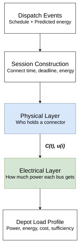
Figure 2.
Binding allocation clip by hour of day in the simulated September 2025 depot (30 units, 1 300 kW pool; duty-matched tier, 423 visits over 1 to 5 September; ). (a) Mean number of buses connected, by state. (b) Share of drawing bus-minutes by the clip that set each bus’s power. Hours with no drawing bus (all buses full, or charging blocked by the time-of-use schedule) are left empty. The figure shows simulated model behaviour, not a measurement.
Figure 2.
Binding allocation clip by hour of day in the simulated September 2025 depot (30 units, 1 300 kW pool; duty-matched tier, 423 visits over 1 to 5 September; ). (a) Mean number of buses connected, by state. (b) Share of drawing bus-minutes by the clip that set each bus’s power. Hours with no drawing bus (all buses full, or charging blocked by the time-of-use schedule) are left empty. The figure shows simulated model behaviour, not a measurement.
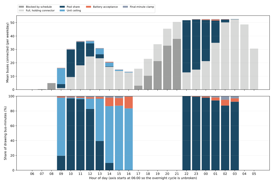
Figure 3.
July 2025 validation. (a) Distribution of energy delivered per session, five days, 286 measured against 216 simulated sessions. (b) Median power per connected bus, overnight (22:00 to 23:59), measured against simulated under pack and spread connector assignment (Section 3.5). (c) Load shape for 16 July, the single day with per-minute telemetry, measured against simulated, with time-of-use-blocked hours shaded.
Figure 3.
July 2025 validation. (a) Distribution of energy delivered per session, five days, 286 measured against 216 simulated sessions. (b) Median power per connected bus, overnight (22:00 to 23:59), measured against simulated under pack and spread connector assignment (Section 3.5). (c) Load shape for 16 July, the single day with per-minute telemetry, measured against simulated, with time-of-use-blocked hours shaded.
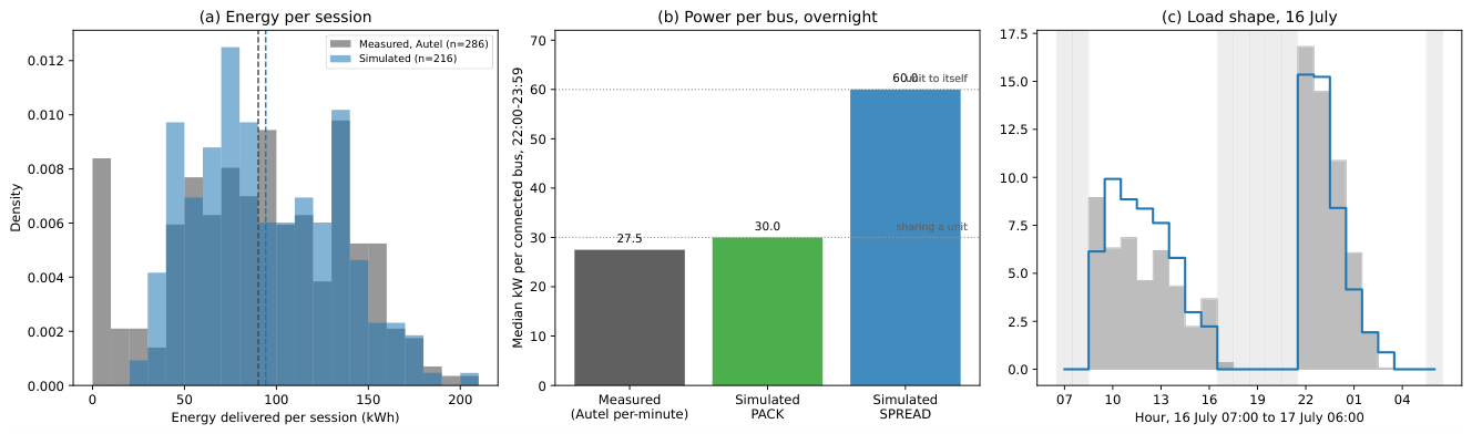
Figure 4.
Five-day site load reconstruction, 14 to 18 July 2025, measured (grid import, solar generation, and BESS discharge combined) against simulated. (a) Load per depot visit by hour of day, absolute power. (b) The same comparison normalised to each series’ own maximum, isolating timing agreement from magnitude; time-of-use-blocked hours are shaded.
Figure 4.
Five-day site load reconstruction, 14 to 18 July 2025, measured (grid import, solar generation, and BESS discharge combined) against simulated. (a) Load per depot visit by hour of day, absolute power. (b) The same comparison normalised to each series’ own maximum, isolating timing agreement from magnitude; time-of-use-blocked hours are shaded.
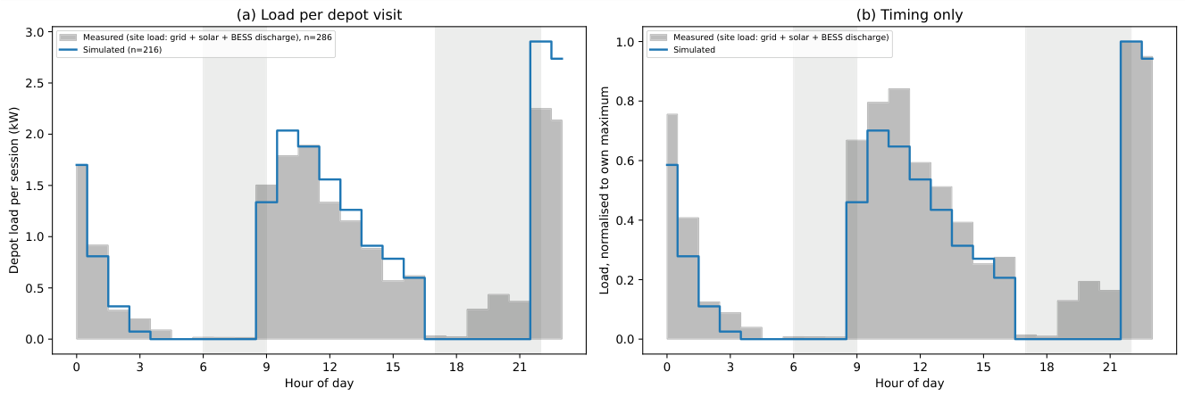
Figure 5.
Charging load per depot visit, 4 September 2025, on the 23-bus like-for-like subset: measured against simulated on both the duty-matched and observed-energy tiers (Section 3.7).
Figure 5.
Charging load per depot visit, 4 September 2025, on the 23-bus like-for-like subset: measured against simulated on both the duty-matched and observed-energy tiers (Section 3.7).
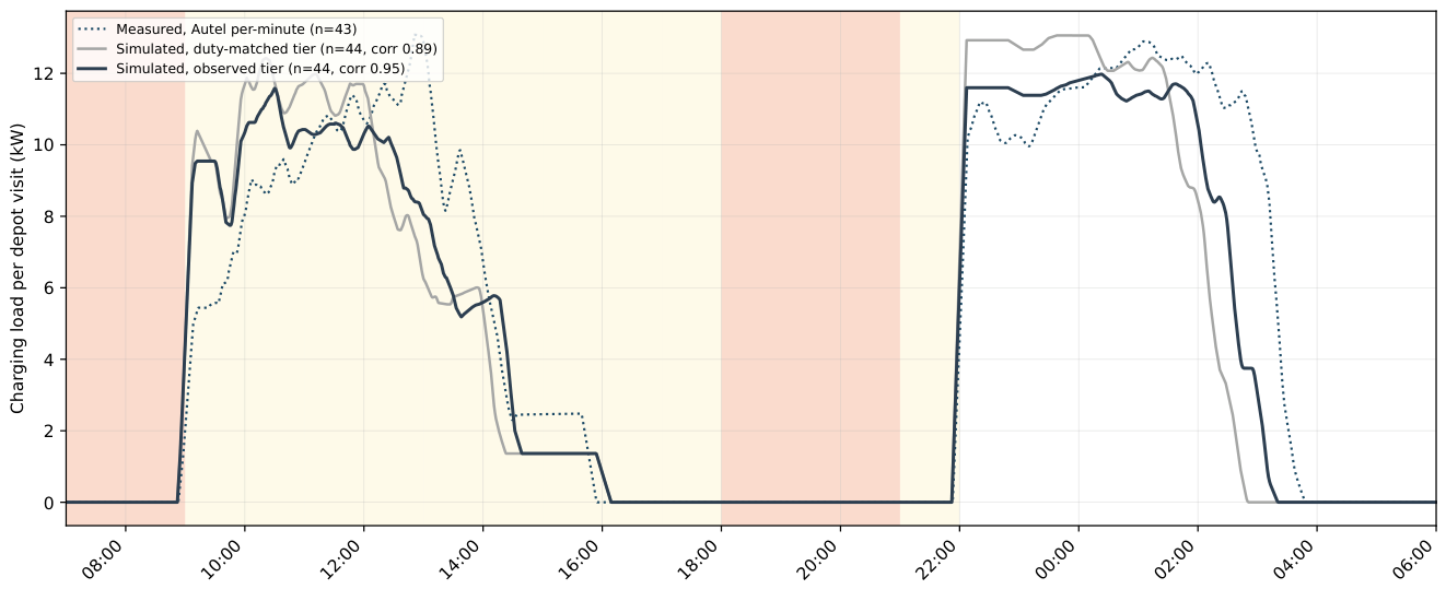
Figure 6.
Depot charging load by hour of day for the seven use-case scenarios (September hardware, observed-energy tier, fleet size 62). The left axis gives load per bus in the fleet and the right axis the equivalent fleet load. The curves are 15-minute means across the five days, so they sit below each scenario’s peak minute in Table 4; scenario 3’s peak minute, 3 166.9 kW, exceeds the contracted notified maximum demand of 3 000 kVA. In the 30 kW scenarios the load drops to zero at 06:00 as buses depart, most of them below full; that shortfall is carried into their next visit.
Figure 6.
Depot charging load by hour of day for the seven use-case scenarios (September hardware, observed-energy tier, fleet size 62). The left axis gives load per bus in the fleet and the right axis the equivalent fleet load. The curves are 15-minute means across the five days, so they sit below each scenario’s peak minute in Table 4; scenario 3’s peak minute, 3 166.9 kW, exceeds the contracted notified maximum demand of 3 000 kVA. In the 30 kW scenarios the load drops to zero at 06:00 as buses depart, most of them below full; that shortfall is carried into their next visit.
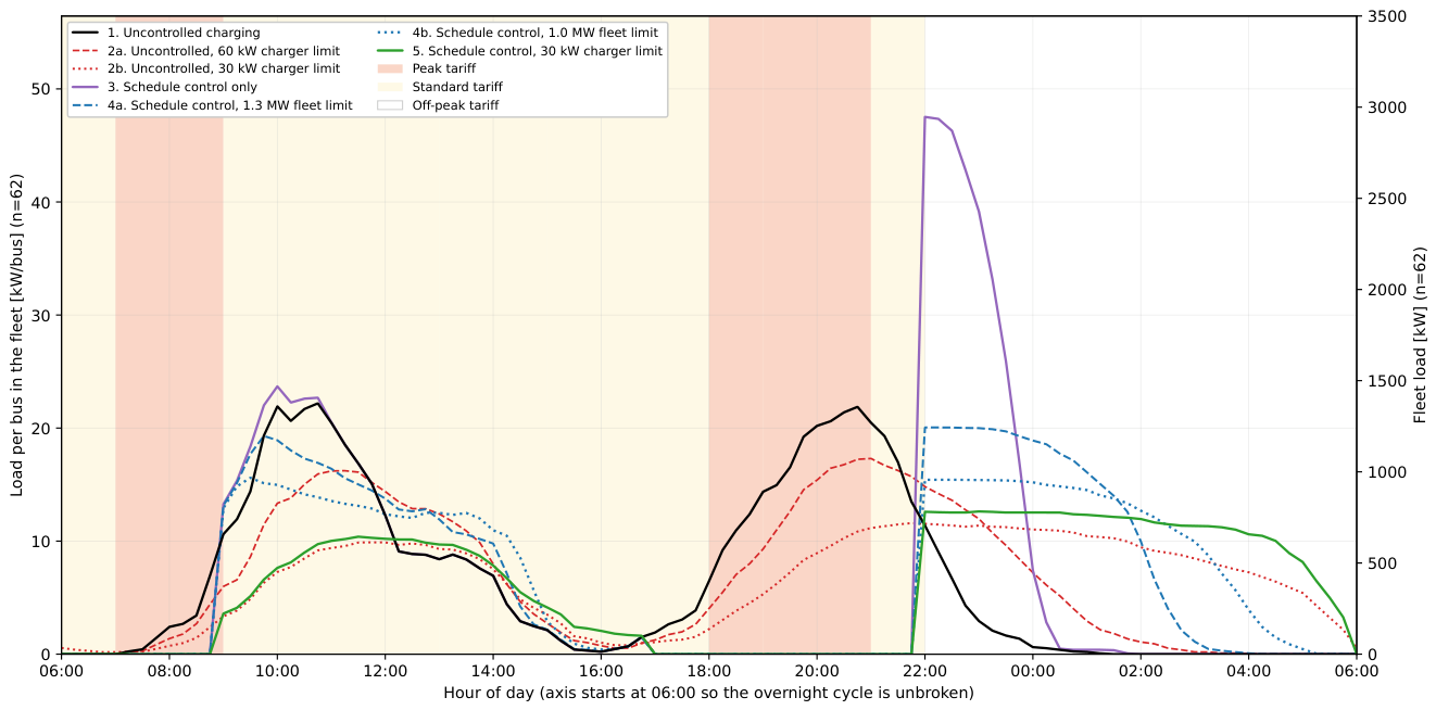
Figure 7.
Depot charging load by hour of day for the seven use-case scenarios on the duty-matched tier (September hardware, fleet size 62), plotted on the same scale as Figure 6.
Figure 7.
Depot charging load by hour of day for the seven use-case scenarios on the duty-matched tier (September hardware, fleet size 62), plotted on the same scale as Figure 6.
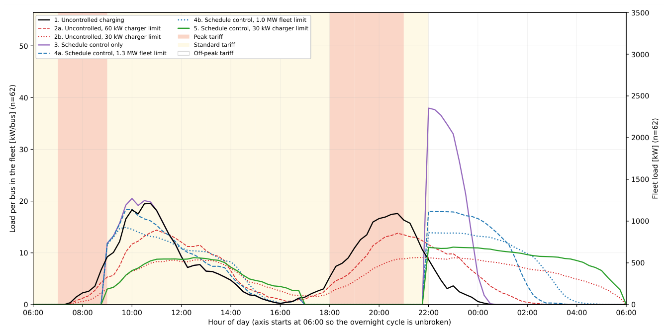

Table 1.
Sensitivity of the September 2025 simulation to the redistribution fraction (30 units, 1 300 kW pool; duty-matched tier, 423 visits over 1 to 5 September). Shares are percentages of the bus-minutes in which a bus was drawing power. All values are simulated.
Table 1.
Sensitivity of the September 2025 simulation to the redistribution fraction (30 units, 1 300 kW pool; duty-matched tier, 423 visits over 1 to 5 September). Shares are percentages of the bus-minutes in which a bus was drawing power. All values are simulated.
| Peak (kW) | Energy (kWh) | Pool (%) | Unit (%) | Battery (%) | Clamp (%) | |
|---|---|---|---|---|---|---|
| 0.25 | 1 209.9 | 40 632 | 90.7 | 7.1 | 1.6 | 0.6 |
| 0.50 | 1 237.1 | 40 632 | 86.8 | 11.0 | 1.6 | 0.7 |
| 0.75 | 1 258.9 | 40 632 | 74.2 | 22.8 | 2.3 | 0.8 |
| 1.00 | 1 300.0 | 40 632 | 61.1 | 34.6 | 3.4 | 0.8 |
Table 2.
Visit-population coverage against charger records, by era and tier.
| Era | Charger records | Duty-matched | Observed-energy | |
|---|---|---|---|---|
| July 2025 (14–18) | 286 | 173 (60 %) | 216 (76 %) | |
| September 2025 (1–5) | 682 | 423 (62 %) | 506 (74 %) |
Table 3.
The seven use-case scenarios (September hardware, 5 weekdays; observed-energy tier, 506 visits, with the duty-matched tier, 423 visits, as a cross-check). Every scenario shares the same physical and electrical-layer features except the three columns varied here. Charger rate is the per-unit rating, shared by the unit’s two connectors.
Table 3.
The seven use-case scenarios (September hardware, 5 weekdays; observed-energy tier, 506 visits, with the duty-matched tier, 423 visits, as a cross-check). Every scenario shares the same physical and electrical-layer features except the three columns varied here. Charger rate is the per-unit rating, shared by the unit’s two connectors.
| Scenario | Time-of-use schedule | Charger rate (kW) | Site pool limit (kW) |
|---|---|---|---|
| 1. Uncontrolled charging | none | 120 | none |
| 2a. Uncontrolled, 60 kW charger limit | none | 60 | none |
| 2b. Uncontrolled, 30 kW charger limit | none | 30 | none |
| 3. Schedule control only | applied | 120 | none |
| 4a. Schedule control + 1.3 MW pool | applied | 120 | 1 300 |
| 4b. Schedule control + 1.0 MW pool | applied | 120 | 1 000 |
| 5. Schedule control + 30 kW | applied | 30 | none |
Table 4.
Outcomes of the seven use-case scenarios on the observed-energy tier (September hardware, 506 visits over 5 weekdays). Sufficiency is the share of sessions not followed by a stranded trip; energy owed is the fleet’s shortfall below full after each bus’s last session (Section 3.4). The monthly bill scales the 5-weekday energy total to 21.5 weekdays per month and adds a fixed demand, network, and service component (Section 3.1); it is not directly comparable to an actual invoice, which bills on metered grid import net of any future solar or storage contribution.
Table 4.
Outcomes of the seven use-case scenarios on the observed-energy tier (September hardware, 506 visits over 5 weekdays). Sufficiency is the share of sessions not followed by a stranded trip; energy owed is the fleet’s shortfall below full after each bus’s last session (Section 3.4). The monthly bill scales the 5-weekday energy total to 21.5 weekdays per month and adds a fixed demand, network, and service component (Section 3.1); it is not directly comparable to an actual invoice, which bills on metered grid import net of any future solar or storage contribution.
| Scenario | Peak (kW) | Sufficiency (%) | Stranded trips | Energy delivered (kWh) | Energy owed (kWh) | Bill (R/month) |
|---|---|---|---|---|---|---|
| 1. Uncontrolled charging | 1 832.2 | 100.00 | 0 | 49 492 | 0 | 876 385 |
| 2a. Uncontrolled, 60 kW charger limit | 1 260.0 | 100.00 | 0 | 49 492 | 0 | 783 424 |
| 2b. Uncontrolled, 30 kW charger limit | 765.0 | 98.02 | 10 | 48 372 | 864 | 665 893 |
| 3. Schedule control only | 3 166.9 | 100.00 | 0 | 49 492 | 0 | 821 208 |
| 4a. Schedule control + 1.3 MW pool | 1 300.0 | 100.00 | 0 | 49 492 | 0 | 657 866 |
| 4b. Schedule control + 1.0 MW pool | 1 000.0 | 99.80 | 1 | 49 483 | 0 | 629 668 |
| 5. Schedule control + 30 kW | 840.0 | 85.38 | 74 | 44 206 | 3 087 | 554 696 |
Table 5.
Duty-matched cross-check of Table 4 (September hardware, 423 visits over 5 weekdays). Columns as in Table 4.
| Scenario | Peak (kW) | Sufficiency (%) | Stranded trips | Energy delivered (kWh) | Energy owed (kWh) | Bill (R/month) |
|---|---|---|---|---|---|---|
| 1. Uncontrolled charging | 1 500.0 | 100.00 | 0 | 40 632 | 0 | 729 203 |
| 2a. Uncontrolled, 60 kW charger limit | 1 020.0 | 100.00 | 0 | 40 632 | 0 | 652 014 |
| 2b. Uncontrolled, 30 kW charger limit | 615.0 | 99.76 | 1 | 40 269 | 327 | 567 324 |
| 3. Schedule control only | 2 520.0 | 100.00 | 0 | 40 632 | 0 | 679 413 |
| 4a. Schedule control + 1.3 MW pool | 1 237.1 | 100.00 | 0 | 40 632 | 0 | 567 448 |
| 4b. Schedule control + 1.0 MW pool | 1 000.0 | 100.00 | 0 | 40 632 | 0 | 546 316 |
| 5. Schedule control + 30 kW | 765.0 | 95.27 | 20 | 38 751 | 1 363 | 498 846 |
Disclaimer/Publisher’s Note: The statements, opinions and data contained in all publications are solely those of the individual author(s) and contributor(s) and not of MDPI and/or the editor(s). MDPI and/or the editor(s) disclaim responsibility for any injury to people or property resulting from any ideas, methods, instructions or products referred to in the content. |
© 2026 by the authors. Licensee MDPI, Basel, Switzerland. This article is an open access article distributed under the terms and conditions of the Creative Commons Attribution (CC BY) license (http://creativecommons.org/licenses/by/4.0/).
Copyright: This open access article is published under a Creative Commons CC BY 4.0 license, which permit the free download, distribution, and reuse, provided that the author and preprint are cited in any reuse.