

Submitted:
01 October 2026
Posted:
06 October 2026
You are already at the latest version
Abstract
Motorcyclists account for ~83.8% of Thailand’s road-traffic deaths, yet fatalities per crash—the metric most relevant to intervention—have rarely been modelled for motorcycles using frameworks that handle both underdispersion and zero-fatality inflation. Building on prior aggregate-level zero-inflated Conway–Maxwell–Poisson (ZICMP) research on Thai road deaths, we compared Poisson, CMP, Zero-inflated Poisson (ZIP), and ZICMP models, each incorporating location-by-collision-type interactions, using seven years of motorcycle crash data (2019-2025; n = 23,335)—to our knowledge the first interaction-based ZICMP analysis of this outcome. The ZICMP-interaction model fit best (AIC = 32,940.71; BIC = 33,367.76; ν ̂ = 2.54, confirming underdispersion). Head-on and fixed-object collisions raised expected fatalities (IRR = 2.77 and 1.69; p < 0.001). Nighttime crashes proved far more lethal than daytime ones (39.6% vs. 25.3% fatal; OR = 0.23, p < 0.001), while April (Songkran) showed the highest non-fatal odds (OR = 1.36, p = 0.002), suggesting its toll stems from crash volume, not severity. Interactions also cut lethality at intersections (head-on, ~37%; IRR = 0.49) and access points (fixed-object, ~70%; IRR = 0.21)—patterns additive models miss. Nighttime open roads, not festivals, emerge as the priority target for motorcycle-safety interventions.
Keywords:
motorcycle fatality severity
; count regression
; Conway–Maxwell–Poisson
; zero inflation
; underdispersion
; interaction effects
; road safety
1. Introduction
Road traffic injuries continue to impose a major public health and economic burden worldwide. The World Health Organization (WHO) identifies road traffic injuries as a leading cause of death globally and notes that road crashes cost most countries around 3% of their gross domestic product (GDP) [1]. Thailand is among the most severely affected nations: in 2021, the WHO ranked Thailand 16th globally and 2nd in Asia for road traffic fatalities, recording an alarming death rate of 25.4 per 100,000 population. The WHO Thailand road safety profile further estimates 18,218 road traffic deaths (RTD) in that year—approximately 50 deaths per day—placing the country among the highest-burden settings globally. The economic toll is correspondingly large; the Thailand Development Research Institute (TDRI) estimates that losses from road traffic accidents during 2015–2019 ranged from approximately 260,000 to 430,000 million baht per year, averaging about 3.5% of GDP [2]. These figures position road safety not merely as a public-health emergency but also as a development and fiscal priority aligned with Sustainable Development Goal 3.6.
Within this burden, motorcyclists are disproportionately represented. The WHO reports that motorcyclists accounted for about 83.8% of all traffic deaths in Thailand in 2021—far exceeding the global figure of roughly 21% for powered two- and three-wheeler users [1]. National surveillance corroborates this pattern: the Department of Disease Control (DDC) recorded 17,477 RTD in 2024, of which 14,144 (≈80%) were motorcycle-related [3], while the Department of Highways reported 55,749 crashes, 31,007 injuries, and 5345 deaths on the national highway network in the same year [4]. These sources differ in coverage—the DDC compiles deaths nationwide across all road types, whereas the Department of Highways captures only its managed network—but both converge on the same conclusion: motorcycle riders bear an outsized share of Thailand’s road fatalities.
To examine this pattern within a single operational dataset, this study draws on official road accident records from Thailand’s Ministry of Transport covering 2019–2025 [5]. After removing duplicate records, the dataset comprises 148,969 reported crashes, 122,989 injuries, and 20,151 deaths across all vehicle types. Crashes involving at least one motorcycle account for 32,651 cases (≈21.9% of all crashes), yet they are associated with 11,140 deaths—roughly 55.3% of all fatalities in the dataset—and 32,654 injuries (≈26.6%). In other words, motorcycles are involved in about one-fifth of crashes but more than half of all deaths, a striking asymmetry consistent with the national pattern reported by the DDC. Figure 1 makes this contrast explicit: panel (a) shows that motorcycle-related crashes do not consistently constitute the largest share of total crashes by vehicle category, whereas panel (b), measured as deaths per 1000 crashes, shows that motorcycle crashes exhibit the highest fatality rate in each year, clearly exceeding all other vehicle categories. Motorcycles may contribute a smaller portion of absolute crash counts, but they produce disproportionately lethal outcomes—an asymmetry that motivates an analysis focused on fatality severity rather than crash occurrence alone.
This divergence implies that analyses focusing only on aggregate crash counts, or on a binary fatal-versus-non-fatal outcome modeled through logistic regression or machine-learning classifiers [6,7], may substantially understate the true burden of motorcycle crashes. A binary outcome collapses severity into a single threshold and therefore cannot represent the distribution of the number of deaths per crash, nor reveal how risk factors shape the magnitude of loss once a crash turns fatal. What is required is an analytical framework that models fatality severity directly—as a count of deaths per crash. Count regression models are well suited to this task because they accommodate non-negative integer outcomes and allow the expected number of fatalities to vary systematically with crash characteristics and contextual conditions.
Modeling the number of deaths per crash raises two statistical challenges that frequently co-occur in road-safety data. First, most crashes are non-fatal, producing a large mass of zero counts (excess zeros). Second, the death count often departs from the Poisson assumption of equidispersion—typically through overdispersion, where variance exceeds the mean [8,9,10], but occasionally through underdispersion [11]. The standard Poisson model can represent neither feature, and the widely used Negative Binomial (NB) model accommodates only overdispersion [12,13,14,15]. The Conway–Maxwell–Poisson (CMP) distribution resolves this limitation through a dispersion parameter ν that flexibly captures both over- and underdispersion, while a zero-inflated formulation adds a structural-zero component that separates “always non-fatal” crashes from those governed by the count process [16]. The zero-inflated Conway–Maxwell–Poisson (ZICMP) regression unifies both mechanisms [17]. A further, largely unaddressed limitation is that risk factors are typically modeled as acting independently, even though the lethality of a given collision type plausibly depends on where it occurs.
The present study addresses these gaps by modeling the number of fatalities per motorcycle crash in Thailand using count regression, comparing Poisson, CMP, and their zero-inflated counterparts, and extending the best-fitting specification with interaction terms between collision type and accident location. As detailed in the sections that follow, the zero-inflated Conway–Maxwell–Poisson model with interaction terms provides the best balance of fit and parsimony among the specifications considered. Fatality risk proves highly sensitive to both collision type and time of day, and—critically—the lethality of a given collision type depends systematically on where it occurs: certain high-risk collision types become markedly less lethal at specific location types, a pattern that models without interaction terms cannot detect. These findings translate directly into spatially targeted, rather than uniformly applied, road-safety interventions. The remainder of the paper is organized as follows. Section 2 reviews the literature on motorcycle crash severity, underdispersed count modeling, and interaction effects. Section 3 describes the data source, screening procedure, and the count regression framework. Section 4 reports the exploratory analysis, model comparison, and estimation results. Section 5 discusses the findings and their policy implications, and Section 6 concludes with limitations and future directions.
2. Literature Review
Motorcyclists are consistently the most vulnerable road users in Thailand, where crashes and fatalities have long been linked to young riders, alcohol use, and helmet non-compliance [6,18,19]. More recent work has broadened this view to roadway and environmental contributors, and the relative weight of behavioral versus infrastructural risk factors remains debated: some studies attribute the bulk of motorcycle fatality risk to rider behavior, while others argue that road geometry, lighting, and traffic control at the crash site are equally, if not more, decisive—a distinction with direct implications for whether interventions should target riders or road design. Internationally, Acosta-González et al. [20] likewise report the highest fatality risk for motorcycles among vehicle types, alongside separately elevated risk at night and in rural areas, lending support to the infrastructural view. Much of the severity literature, however, treats the outcome as categorical—binary or ordinal—and models it with logistic regression, mixed logit, or machine-learning classifiers [7,21,22], an approach that identifies risk factors but cannot represent the distribution of the number of deaths per crash, motivating a count-based formulation. Table 1 summarises representative count-regression studies in road-safety and insurance research, organised by outcome variable, covariates, count model, evaluation criteria, and their principal distinction from the present study.
Collectively, these studies trace a clear methodological progression. Early work relied on the Poisson model and its negative binomial (NB) extension to accommodate the overdispersion that is common in crash-frequency data [23]. Spatial and spatio-temporal extensions have also been proposed to capture correlation across road segments and interactions between roadway and environmental factors [25]. As researchers increasingly encountered data exhibiting underdispersion or clustering, more flexible specifications were adopted, including the CMP model, which accommodates both over- and underdispersion through a single dispersion parameter, and random-effects formulations such as the clustered COM–Poisson model with gamma random effects [24]. A parallel strand of literature addressed the excess-zero problem that frequently arises when the response is the number of fatalities per crash. This motivated zero-inflated models, which separate crashes that are structurally non-fatal (i.e., can never produce a death, regardless of circumstances) from those governed by a random count process—specifications including Zero-inflated Poisson (ZIP), ZINB, ZICMP, and ZIHTCMP have all been applied in this spirit [11,12,26,27]. Model selection across these studies has typically been guided by goodness-of-fit comparisons, information criteria (AIC, BIC), and formal statistical tests—including likelihood-ratio statistics and the Vuong test, which compares non-nested models—and, more recently, by out-of-sample validation and empirical-Bayes ranking [12,28].
Despite this maturation, two limitations persist in the existing literature. First, although zero-inflated and dispersion-flexible models such as ZICMP have been applied to aggregate or general crash data, their use for motorcycle-specific fatality counts—where simultaneous underdispersion and zero inflation are particularly salient—remains scarce. Second, and more importantly, prior studies have almost exclusively specified covariates in an additive (main-effects-only) fashion. Where interaction effects have been examined, the focus has been on roadway-by-weather interactions in the context of freeway crash frequency [25], leaving interactions among crash type, location, and other risk factors in the context of fatality severity unexplored—particularly for motorcycles. A head-on impact on an open road, for instance, plausibly carries very different consequences from one at a speed-controlled intersection [20,26], yet no study to date has tested this directly for motorcycle fatalities. The present study addresses both gaps by fitting Poisson, CMP, ZIP, and ZICMP regressions to deaths per motorcycle crash, explicitly incorporating interaction terms, and evaluating the competing specifications through a comprehensive set of criteria—the likelihood-ratio test, AIC, BIC, and the score test for zero inflation. Its contributions are threefold: (i) it is, to our knowledge, among the first studies to apply ZICMP regression to motorcycle-specific fatality severity in Thailand; (ii) it jointly addresses excess zeros and underdispersion rather than treating them in isolation; and (iii) it quantifies location-by-collision-type interactions that translate directly into targeted road-safety interventions.
3. Methods
3.1. Study Design and Data Source
This was a retrospective, observational study based on the open road-crash dataset published by Thailand’s Ministry of Transport through its open-data portal (datagov.mot.go.th), covering the period 2019–2025. The records are compiled from on-scene reports filed by traffic police and road authorities operating under the Department of Rural Roads (DRR), the Department of Highways (DOH), and the Expressway Authority of Thailand (EXAT). Each record documents the circumstances of a crash, including vehicle types involved, accident location and road geometry, probable cause, weather and lighting conditions, time of occurrence, and the resulting counts of injuries and fatalities. Because the data are publicly available and contain no information that could identify individual persons, the study did not involve direct contact with participants and required neither ethical approval nor informed consent.
3.2. Outcome Variable and Covariates
The outcome variable was fatality severity, defined as the number of deaths per motorcycle crash, a non-negative count ranging from 0 to 8. The covariates were drawn from established crash-severity frameworks and prior peer-reviewed studies and were organized into four conceptual domains: crash characteristics (collision type and accident location), causal factors (probable cause), environmental conditions (weather), and temporal factors (year, month, and time of day). All covariates were categorical. Their operational definitions, the consolidation of original Thai-language field values into analytic categories, and the frequency distribution of each category are summarized in Table 2. For each categorical predictor, the most frequent and substantively interpretable level was set as the reference category for the regression models.
3.3. Data Screening and Analytical Sample
The construction of the analytical sample followed a sequential screening procedure, summarized in Figure 2. The raw dataset comprised 150,759 crash records. Duplicate records were removed in two steps: first, 1702 records sharing an identical accident code were removed; second, 88 records sharing identical date, time, latitude, and longitude coordinates were removed, leaving 148,969 unique crashes across all vehicle types. The sample was then restricted to motorcycle-involved crashes—defined as any crash involving at least one motorcycle—yielding 32,651 records.
To address missing values, complete-case screening was applied to the analysis variables only, rather than listwise deletion across all available fields. This decision retained 24,784 records. By comparison, deletion based on missingness in any field—including variables not used in the analysis—would have retained only 21,079 records, discarding 3705 more crashes (11,572 vs. 7867 removed from the 32,651 motorcycle-involved records) and disproportionately removing certain annual cohorts, which would have biased temporal comparisons.
Finally, to limit the instability introduced by sparsely populated categories, predictor levels representing fewer than 0.5% of the screened motorcycle sample (n = 24,784; <124 records) were excluded. This step removed 1449 records spanning rare levels of accident location, probable cause, and collision type. One exception was made: the cause category roadway fixed object (n = 110) fell marginally below this threshold but was retained because of its theoretical relevance and its significant association with fatality counts in preliminary analyses. The final analytical sample comprised 23,335 motorcycle-related crashes spanning seven annual cohorts (2019–2025), ranging from 2953 crashes in 2022 to 3628 in 2019.
3.4. Statistical Models
To accommodate the joint presence of excess zeros and underdispersion observed in the fatality count, four count-regression specifications of increasing flexibility were fitted and compared: the Poisson model as a baseline; the CMP model, which relaxes the equidispersion assumption; the ZIP model, which isolates the contribution of excess zeros; and four count-regression specifications were fitted and compared, each incorporating an identical set of covariates—including an interaction term between accident location and collision type—so that the comparison isolated the effect of distributional and zero-inflation assumptions rather than covariate structure.
3.4.1. Poisson Regression
Let Yi denote the number of fatalities in the i-th motorcycle-related crash (i = 1, …, n). Under the Poisson regression framework, the fatality count is assumed to follow a Poisson distribution with mean λi > 0:
A fundamental property of the Poisson distribution is equidispersion, whereby the conditional mean and variance are equal: E(Yi) = Var(Yi) = λi. The expected fatality count is linked to a set of explanatory variables xi—comprising road characteristics, weather and environmental conditions, crash characteristics, and temporal indicators—through a log-link function:
where β is the vector of regression coefficients. Parameters are estimated via maximum likelihood (ML). The log-likelihood function, summed over n observations, is:
Exponentiated coefficients, exp(βj) are interpreted as incidence rate ratios (IRRs), representing the multiplicative change in the expected fatality count associated with a one-unit increase in the j-th covariate, or relative to a reference category for indicator variables. Although the Poisson model provides a natural baseline for count data, the equidispersion constraint renders it inappropriate when the observed variance departs substantially from the mean.
3.4.2. Conway–Maxwell–Poisson (CMP) Regression
To relax the equidispersion constraint of the Poisson model, we employ the CMP distribution [29,30], a two-parameter generalization capable of accommodating both overdispersion and underdispersion. The probability mass function of the CMP distribution is:
where is a normalizing constant, and ν > 0 is the dispersion parameter. When ν = 1, the CMP reduces to the standard Poisson distribution. Values ν < 1 yield overdispersion, whereas values ν> 1 yield underdispersion, with the ratio . The approximate mean and variance are:
In the regression framework, the location parameter is modeled via a log-link:
The dispersion parameter is held constant across all observations (νi = ν), consistent with the constant-dispersion specification of the COMPoissonReg package [31]. The log-likelihood function for the CMP regression is therefore:
Parameters are estimated by maximum likelihood using iterative numerical optimization [16]. To assess whether the dispersion parameter departs significantly from unity—that is, to test whether the Poisson model is preferred over CMP—a likelihood ratio test (LRT) is conducted under H0: ν = 1 versus H1: ν ≠ 1, with test statistic:
where denotes the ML estimates under the Poisson model. A significant LR statistic indicates that the CMP model provides a superior fit by accounting for the observed degree of dispersion.
3.4.3. Zero-Inflated Poisson (ZIP) Regression
As an intermediate specification, the ZIP model [32] is considered to isolate the contribution of zero-inflation from that of non-equidispersion. The ZIP model assumes a two-component mixture: with probability πi, an observation arises from a structural-zero state; with probability 1 − πi, it is drawn from a Poisson (λi) distribution. The zero-inflation probability is modelled via a logistic link, logit (πi) = . The ZIP model is nested within the ZICMP model (obtained when ν = 1), permitting a direct LRT of whether the CMP count structure is necessary given that zero-inflation has been accounted for.
3.4.4. Zero-Inflated Conway–Maxwell–Poisson (ZICMP) Regression
Motorcycle crash fatality data typically contain a substantial proportion of zero counts corresponding to non-fatal accidents and may simultaneously exhibit dispersion that is inconsistent with the Poisson assumption. To jointly accommodate excess zeros and flexible dispersion, we adopt the ZICMP regression proposed by Sellers and Raim [17]. The model assumes a two-component mixture process: with probability πi, the observation is generated from a structural-zero state (an accident that can never result in a fatality under any circumstance); with probability 1 − πi, the observation is drawn from a CMP(λi, ν) distribution, which itself assigns positive probability to a zero count (a non-fatal accident arising from the count process). The resulting probability mass function is:
where and .
Pr(Yi = 0) = πi + (1 − πi)fCMP(0; λi; ν)
Pr(Yi = yi) = (1 − πi)fCMP(yi; λi; ν), yi = 1, 2, …
The ZICMP model is specified through three sub-models. The count component relates the CMP location parameter to crash-level covariates via a log-link:
The dispersion parameter is held constant across all observations (νi = ν), consistent with the constant-dispersion specification adopted in the CMP component of this study. The zero-inflation component models the probability of belonging to the structural-zero state via a logistic link:
where zi is a vector of covariates (which may overlap with or differ from xi) and γ is the corresponding coefficient vector. The full log-likelihood function for the ZICMP regression is:
Parameters are estimated by maximum likelihood. In the count component, exponentiated coefficients exp(βj) are interpreted as IRRs for the fatality count among crashes that belong to the at-risk (non-structural-zero) group. In the zero-inflation component, exponentiated coefficients exp(γj) are interpreted as odds ratios for the probability of belonging to the structural-zero state. The ZICMP model nests both the CMP model (when πi = 0) and the ZIP model (when ν = 1), with model selection guided by the LRT.
To capture the joint effect of road location and collision type on fatality counts, the count component additionally incorporates interaction terms between accident location and accident type. These terms allow the effect of a given collision type to vary systematically across road location categories, providing a more nuanced assessment of how crash dynamics and contextual setting jointly influence severity outcomes (see Table 2 for retained covariate levels).
3.5. Model Diagnostics and Selection
Model adequacy and relative performance were assessed through a sequence of formal tests and information criteria. First, a score test for excess zeros [33] was applied to determine whether a zero-inflation component was warranted. Second, likelihood-ratio tests were used for nested comparisons: Poisson versus CMP(H0: ν = 1), CMP versus ZICMP, and ZIP versus ZICMP. Third, the Akaike Information Criterion (AIC) [34] and the Bayesian Information Criterion (BIC) were used to compare overall fit and parsimony across both nested and non-nested specifications, with BIC given particular weight in view of the large sample size (n = 23,335).
Prior to fitting zero-inflated models, the presence of excess zeros in the fatality count distribution is formally assessed using the score test proposed by Van den Broek [33]. Under the null hypothesis H0: π = 0—that is, all observed zero counts arise from the standard Poisson count process, and no structural-zero component is present—the score statistic is defined as:
where n is the total number of observations, n0 is the observed number of zero counts, is the sample mean of the fatality counts (serving as the Poisson parameter estimate under H0), and = is the estimated probability of a zero count under the Poisson model. In large samples, S follows asymptotically a chi-squared distribution with one degree of freedom. Rejection of H0 provides evidence that the proportion of zeros in the data exceeds what the Poisson distribution can accommodate, thereby justifying the inclusion of a zero-inflation component. This test is implemented via the zero.test() function in the vcdExtra package [35].
For any pair of nested models, the likelihood ratio test (LRT) statistic is defined as:
where 𝓵1 and 𝓵0 are the maximised log-likelihoods of the full and restricted models, respectively, and ∆k is the difference in the number of free parameters. Three specific applications are employed in this study: (i) H0: ν = 1 to assess whether CMP is preferred over Poisson; (ii) H0: γ = 0 to assess whether zero-inflation is warranted over the standard CMP model; and (iii) H0: ν = 1 within the ZICMP framework to assess whether ZICMP is preferred over ZIP. Rejection of each null hypothesis at the 5% significance level indicates that the more flexible model is supported by the data.
LR = 2(𝓵1 − 𝓵0)~χ2(df = ∆k)
For comparing both nested and non-nested models, the Akaike Information Criterion (AIC) and the Bayesian Information Criterion (BIC) are reported:
where 𝓵 is the maximised log-likelihood, k is the number of estimated parameters, and n is the sample size. Lower values of both criteria indicate a preferable balance between goodness of fit and model parsimony [34,36]. Because BIC imposes a heavier penalty for model complexity than AIC—a distinction that becomes consequential at the present sample size of n = 23,335—both criteria are reported to provide a comprehensive basis for model comparison.
AIC = −2𝓵 + 2k
BIC = −2𝓵 + k × ln(n)
3.6. Statistical Software
All analyses were conducted in R version 4.5.1 [37]. The Poisson model was fitted using glm() (MASS package); the ZIP model using zeroinfl() (pscl package; Zeileis et al., 2008); and the CMP and ZICMP models—including dispersion testing, zero-inflation testing, and coefficient inference—using glm.cmp() in the COMPoissonReg package (Sellers et al., 2026), which supports constant-dispersion CMP and ZICMP estimation via maximum-likelihood optimization with the L-BFGS-B algorithm. The score test for excess zeros was implemented via zero.test() in the vcdExtra package.
4. Results
The outcome variable Y—the number of deaths per motorcycle crash—is a non-negative integer with an excess of zeros, motivating zero-inflated and underdispersed count specifications. Across the final sample of 23,335 motorcycle-related crashes (2019–2025), Y ranged from 0 to 8, with a mean of 0.3395 and a variance of 0.3147. The variance-to-mean ratio of 0.927 (<1) confirms underdispersion, while 16,316 crashes (69.92%) recorded no fatality, 6231 (26.70%) one, 696 (2.98%) two, and 92 (0.39%) three or more. This joint presence of underdispersion and excess zeros confirms the need for a CMP-based, zero-inflated framework.
Descriptive frequencies and fatality severity by covariate are summarized in Table 2. Two columns are reported alongside the conventional frequency distribution (n and %): the mean number of deaths per crash and the percentage of crashes involving at least one fatality [% fatal (≥1)], which jointly characterize the severity profile of each subgroup and anticipate the underdispersed, zero-inflated structure of the response. Across collision types, head-on crashes were the most lethal, exhibiting the highest mean deaths per crash (0.577) and fatality rate (47.5%) despite accounting for only 9.89% of the sample, whereas the predominant rear-end category (61.02%) was comparatively less severe (0.285; 25.3%). Marked heterogeneity was also evident across the remaining covariates: night-time crashes were substantially more severe than daytime crashes (0.448 vs. 0.285; 39.6% vs. 25.3%), adverse weather elevated severity relative to normal conditions (0.439 vs. 0.335), and crashes on curves carried higher fatality risk than those on straight segments (0.437 vs. 0.331).
A particularly noteworthy temporal pattern emerged for the month covariate: April and December—Thailand’s principal festival periods (Songkran and New Year)—recorded the two largest crash volumes (16.28% and 14.46%, respectively) yet the two lowest mean deaths per crash (0.247 and 0.276) and fatality rates (22.4% and 24.7%). This decoupling of crash frequency from fatality severity, in which an unusually high number of non-fatal (zero-death) crashes concentrates within specific subgroups, illustrates precisely the excess-zero mechanism that a zero-inflation component is designed to capture, and motivates the inclusion of temporal terms in the zero-inflation sub model.
4.1. Model Comparison and Selection
Prior to fitting the zero-inflated specifications, the score test for excess zeros confirmed that a zero-inflation component was warranted (p < 0.001), rejecting the null hypothesis that the observed zero counts arise solely from a standard Poisson process. As shown in Table 3, four count models were compared using log-likelihood, AIC, and BIC. The ZICMP model provided the best overall balance of fit and parsimony, achieving the lowest AIC (32,940.71) and BIC (33,367.76) with a log-likelihood of −16,417.35, outperforming Poisson, CMP, and ZIP across all criteria. Relative to the Poisson baseline, ZICMP improved the log-likelihood by 418.9 units (from −16,836.24 to −16,417.35). The estimated dispersion parameter was ν = 2.54 (SE = 0.0873). Because ν > 1 in the Conway–Maxwell–Poisson parameterization corresponds to underdispersion, this estimate points in the same direction as the descriptive variance-to-mean ratio of 0.927 (<1). The two quantities are not numerically comparable—the variance-to-mean ratio is a marginal, unconditional summary of the raw counts, whereas ν is a conditional dispersion parameter estimated after adjustment for covariates and the zero-inflation component—but both indicate that the equidispersion assumption of the Poisson model is untenable. Collectively, these results identify ZICMP as the best-fitting model, providing the flexibility required for underdispersed, zero-inflated motorcycle fatality counts. Nested model comparisons via likelihood-ratio tests (LRT) corroborated this ranking. CMP was strongly preferred over Poisson (LR = 172.78, df = 1, p < 0.001), confirming that the dispersion parameter departs significantly from unity. ZICMP was preferred over CMP (LR = 665.00, df = 13, p < 0.001), confirming that the zero-inflation component contributes significantly beyond the CMP count process alone. ZICMP was also preferred over ZIP (LR = 499.76, df = 1, p < 0.001), confirming that allowing ν to depart from 1 significantly improves fit once zero-inflation has been accounted for. Taken together, these tests indicate that neither dispersion adjustment nor zero-inflation alone suffices; both mechanisms are required jointly.
4.2. Interpreting the Best Model and Key Factors
The ZICMP model was identified as the most suitable specification, effectively capturing underdispersion and separating covariates influencing fatality occurrence (zero part) from those influencing fatal severity (count part). As exhibited in Table 4, the odds ratios (zero part) and incidence rate ratios (count part) with 95% confidence intervals reveal distinct effects on the two components. Each part is interpreted as follows.

Table 5.
Observed and model-predicted fatality counts for head-on and fixed-object collisions across accident locations.
Table 5.
Observed and model-predicted fatality counts for head-on and fixed-object collisions across accident locations.
| Location | Collision Type |
n | Observed Mean |
λ(Main) | E(Y), Main |
λ (with Interaction) |
E(Y), with Interaction |
B (Interaction) |
IRR [95% CI] |
p |
|---|---|---|---|---|---|---|---|---|---|---|
| Straight (ref) | Head-on | 1554 | 0.583 | 1.873 | 0.931 | - | - | - | - | - |
| Curve | Head-on | 375 | 0.731 | 2.268 | 1.037 | 2.620 | 1.122 | 0.1445 | 1.16 [0.88, 1.51] |
0.290 |
| Access point | Head-on | 257 | 0.432 | 2.021 | 0.972 | 1.499 | 0.816 | −0.2991 | 0.74 [0.52, 1.06] |
0.100 |
| Intersection | Head-on | 123 | 0.342 | 1.735 | 0.891 | 0.846 | 0.563 | −0.7183 |
0.49 [0.31, 0.76] |
0.001 |
| Straight (ref) | Fixed object | 1586 | 0.441 | 1.146 | 0.690 | - | - | - | - | - |
| Curve | Fixed object | 146 | 0.432 | 1.385 | 0.779 | 1.108 | 0.675 | −0.2250 | 0.80 [0.54, 1.17] |
0.250 |
| Access point |
Fixed object |
25 | 0.120 | 1.237 | 0.725 | 0.262 | 0.225 | −1.5513 |
0.21 [0.06, 0.77] |
0.019 |
| Intersection | Fixed object | 18 | 0.444 | 1.062 | 0.657 | 1.094 | 0.670 | 0.0304 | 1.03 [0.39, 2.72] |
0.951 |
Note. Predictions = model-implied E(Y) from the fitted CMP count component, computed via the CMP normalizing constant (Shmueli et al., 2005); λ (the rate parameter before adjustment for dispersion) is not reported here as it can differ substantially from E(Y) under strong underdispersion. β = interaction-term coefficient; IRR = interaction incidence rate ratio; CI = confidence interval. Percentage reductions cited in the text are calculated as (E(Y)main − E(Y)interaction)/E(Y)main.
4.2.1. Count Part (Fatality Severity)
In the count component, which models the expected number of deaths given the at-risk process, collision type was the dominant driver. Head-on collisions carried the largest effect, sharply increasing the expected fatality count relative to rear-end crashes (IRR = 2.77, 95% CI: [2.48, 3.09]), followed by collisions with a fixed object (i.e., the collision-type category; IRR = 1.69, 95% CI: [1.50, 1.91]) and run-off-road crashes (IRR = 1.16, 95% CI: [1.06, 1.26]). Crashes on curves carried higher expected counts than straight roads (IRR = 1.21, 95% CI: [1.02, 1.44]), and adverse weather raised expected counts relative to normal conditions (IRR = 1.18, 95% CI: [1.04, 1.33]). Among probable causes, roadway fixed object (IRR = 0.33, 95% CI: [0.20, 0.55]) and environment/animals (IRR = 0.87, 95% CI: [0.81, 0.95]) were associated with lower counts than human speeding. After adjustment, fatality counts were significantly lower than the 2019 baseline in most subsequent years (IRRs = 0.80–0.86), indicating a modest downward trend net of compositional differences.
4.2.2. Zero Part (Non-Fatality)
In the zero-inflation component, which models the odds of a crash being structurally non-fatal, time of day and month were significant. Nighttime crashes were far less likely to be non-fatal than daytime crashes (OR = 0.23, 95% CI: [0.18, 0.29]), confirming the elevated fatal risk associated with reduced visibility and delayed emergency response after dark; descriptively, 39.6% of nighttime crashes were fatal versus 25.3% by day. Month effects were pronounced: relative to January, every month from February through November except April showed significantly lower odds of being non-fatal (i.e., higher per-crash fatal risk; ORs = 0.29–0.51). April—the Songkran festival period—was the sole exception, exhibiting significantly higher non-fatal odds (OR = 1.36, 95% CI: [1.12, 1.65]), indicating that although crashes surge during Songkran, each is less likely to be fatal. December did not differ significantly from January (OR = 1.10, p = 0.362). Although December, like April, exhibited elevated crash volume with descriptively lower severity (Table 2), this pattern did not persist after adjustment for collision type, weather, and other covariates, suggesting that December’s apparent non-fatal excess was attributable to compositional differences in crash characteristics rather than a genuine calendar-driven effect independent of them. This challenges the prevailing misconception that Thai festivals are inherently more fatal, a belief amplified by intensive media coverage.
4.2.3. Interaction Effects
Table 5 focuses on head-on and fixed-object collisions—the two collision types with the largest main-effect IRRs in Table 4—to test whether their elevated lethality is further shaped by accident location. Two location-by-type interactions were significant (Table 5), indicating that road context substantially moderates the lethality of high-risk crash types beyond what the additive main effects alone predict. At intersections, the elevated fatal risk associated with head-on collisions was significantly attenuated (interaction IRR = 0.49, 95% CI: [0.31, 0.76]; p = 0.001): the model-implied expected fatality count fell from 0.891 deaths per crash under the additive main-effect specification to 0.563 once the interaction was incorporated—a reduction of roughly 37%—consistent with the speed-reducing effect of intersection traffic control. A parallel but stronger pattern emerged for fixed-object collisions at access points (interaction IRR = 0.21, 95% CI: [0.06, 0.77]; p = 0.019), where the expected fatality count fell from 0.725 to 0.225—a reduction of nearly 70%—reflecting the markedly lower operating speeds of entry/exit transitions. By contrast, curve × head-on, the cell with both the highest observed mean fatality count (0.731 deaths per crash) and the highest model-implied expected count among all eight cells (E(Y) = 1.037 under the additive specification), showed no significant interaction (interaction IRR = 1.16, 95% CI: [0.88, 1.51]; p = 0.290): its extreme lethality is fully explained by the combination of the head-on and curve main effects, with curves offering no additional moderating context. The remaining location × type combinations were similarly non-significant, implying a largely additive structure elsewhere in the model.
5. Discussion
This study modelled motorcycle crash fatality severity as a count of deaths per crash across a seven-year national dataset from Thailand (2019–2025; n = 23,335), motivated by two statistical features that render standard count models inadequate: underdispersion and a heavy inflation of zero-fatality records. The ZICMP-interaction model provided the best balance of fit and parsimony among four competing specifications, and its two-part structure revealed qualitatively distinct sets of risk factors governing whether a crash is structurally non-fatal and how many deaths it produces when it is not. Three sets of findings warrant particular attention: the dominance of collision type and, to a lesser extent, accident location (curve versus straight) in shaping the expected death toll; the extraordinary elevation of fatal risk at night, independent of crash characteristics; and two significant location-by-collision-type interactions that imply road context materially moderates the lethality of the most dangerous crash types, with direct consequences for how countermeasures should be targeted.
5.1. Model Performance and Methodological Contribution
The clear superiority of the ZICMP-interaction model over Poisson, CMP, and ZIP on both AIC and BIC—with BIC imposing a heavier parsimony penalty that becomes consequential at this sample size—demonstrates that neither dispersion flexibility nor zero-inflation alone suffices: both mechanisms must be addressed jointly. The ZICMP regression proposed by Sellers and Raim [17] was specifically designed to unify these two features within a single framework, yet its application to motorcycle-specific fatality counts—where simultaneous underdispersion and high structural-zero proportions are particularly salient—has remained largely unexplored. The present study addresses this gap in two important respects. First, the estimated dispersion parameter ( = 2.54) substantially exceeds unity, departing from the Poisson model’s equidispersion assumption, and is consistent with the strong underdispersion documented for fatality-per-crash outcomes in mixed-road-user datasets. This pattern is suggestive of a data-generating process bounded by the physical mechanics of a single-rider collision: unlike car crashes, where the death toll can vary widely with occupancy, a motorcycle crash offers a comparatively narrow range of plausible outcomes, and this structural regularity is precisely what the CMP framework is built to accommodate. Second, by incorporating interaction terms within the ZICMP-interaction model’s count component, this study advances beyond the additive-only specifications—lacking location-by-collision-type interaction terms—that have characterised prior applications of CMP-family models in the road-safety literature [26,27], enabling a more nuanced assessment of how crash configuration and road environment jointly govern fatal outcomes. The two-part structure of the ZICMP-interaction model further proved analytically productive: the covariates governing the structural non-fatality process and those governing the expected death toll among at-risk crashes were substantively distinct, underscoring that collapsing the outcome to a binary fatal/non-fatal indicator—as in logistic regression or machine-learning classifiers [6,7]—would conceal information directly relevant to intervention design. In practical terms, a binary classifier might correctly flag a head-on collision as high-risk yet remain silent on whether that risk is meaningfully reducible by intersection design—information that determines whether limited road-safety budgets are better directed toward speed-control infrastructure or toward broader helmet-compliance enforcement.
5.2. Collision Type and the Dominance of Head-On Crashes
In the count component, head-on collisions emerged as the single most lethal crash configuration relative to the rear-end reference category, nearly tripling the expected number of deaths per at-risk crash. This result is mechanistically unsurprising: a head-on impact between a motorcycle and an opposing vehicle compounds the closing speeds of both parties, eliminates the deceleration distance that softens rear-end impacts, and leaves the unenclosed rider entirely exposed to the full kinetic energy of the collision. What is notable is the cross-methodological consistency of this finding in the Thai context specifically. Se et al. [22], employing a mixed ordered probit framework on Thai highway data, identified head-on crashes as a temporally stable predictor of fatal and serious injuries across all four annual sub-models from 2016 to 2019, in both daytime and nighttime settings. Using an entirely different approach—Random Forest classifiers with SHAP-based importance ranking—Sum et al. [7] similarly found head-on collisions to consistently carry strong positive SHAP values across all four urban–rural and day–night scenarios in Thailand. The convergence of a parametric count model, an ordered severity model, and a machine-learning classifier on the same conclusion across overlapping Thai datasets substantially strengthens the empirical case that head-on crashes represent a persistent and cross-methodologically robust safety priority, rather than an artefact of any particular modelling choice.
5.3. Accident Location and Environmental Conditions
Beyond collision type, road environment shaped the expected fatality count in consistent and interpretable ways. Fixed-object collisions produced the second-largest elevation in expected deaths among crash types, a finding corroborated by Aristizábal et al. [38], who identified impact with fixed roadside objects as one of the strongest correlates of fatal motorcycle trauma in a case-control study conducted in Medellín, Colombia, underscoring the cross-national relevance of clear-zone and forgiving roadside treatments as a safety priority. Crashes on curved segments carried higher expected fatality counts than those on straight roads, consistent with Chang et al. [39], who reported elevated fatality probability on curved and sloped county roads in Hunan, China, and with Sum et al. [7], who similarly identified horizontal curvature as a positive predictor of crash severity in rural daytime settings in Thailand. The underlying mechanism is well established: curves restrict sight distance, demand continuous lateral control inputs, and reduce the margin for error in the event of a handling perturbation—demands that are particularly acute for unenclosed motorcycle riders. Adverse weather conditions likewise elevated expected fatality counts, consistent with Sangkharat et al. [40], whose nationwide time-series analysis of Thai ambulance-dispatch data confirmed that rainfall significantly increases crash frequency, likely through reduced tyre–road friction, impaired visibility, and extended braking distances.
5.4. Temporal Trends
Year-on-year fixed effects in the count component revealed a consistent, statistically significant reduction in expected fatality counts relative to the 2019 baseline across most subsequent years, with 2020 exhibiting the sharpest decline. This pattern is consistent with the broader reduction in road traffic fatalities documented across Southeast Asia during the COVID-19 pandemic period, when national mobility restrictions substantially curtailed traffic volumes and reduced physical exposure to crash risk on public roads [1,3]. The persistence of modestly lower fatality counts beyond the lockdown period—extending through 2021, 2022, 2024, and 2025—is cautiously encouraging and may reflect the cumulative effects of road safety investments under Thailand’s Road Safety Master Plan alongside structural changes in travel patterns following the pandemic. However, the non-significant estimate for 2023 (IRR = 0.92, p = 0.113) warrants continued monitoring, as a partial return toward baseline severity in that year is consistent with the traffic volume recovery documented in national transportation statistics following the removal of pandemic restrictions. In practical terms, this trajectory offers a cautious but important counternarrative to public perceptions shaped by rising crash headlines: the underlying severity of each individual motorcycle crash has, if anything, been easing over this period, even as absolute crash and fatality counts respond to broader shifts in traffic volume. Importantly, these year effects do not alter the substantive interpretation of other covariates in the model, but they confirm that the fatality-reduction trend observable at the national aggregate level is also detectable at the crash-level count after controlling for compositional differences in crash type, location, cause, and environmental conditions.
5.5. Nighttime Fatal Risk
The most striking finding in the zero-inflation component was the effect of time of day. Nighttime crashes were far less likely to be structurally non-fatal than their daytime counterparts—an odds ratio implying that, all else equal, a crash occurring at night carries approximately fourfold higher odds of producing at least one fatality. This effect substantially exceeds the elevation in nighttime fatal risk reported by Acosta-González et al. [20], who found significantly higher fatality odds during nighttime relative to daytime hours in Ecuador; and is consistent in direction with Se et al. [22], who found that the proportion of fatal injuries in nighttime motorcycle crashes in Thailand (40.21%) exceeded that in daytime crashes (26.42%) by more than 13 percentage points across four consecutive annual cohorts, and with Chang et al. [39], who reported that daylight reduced the probability of motorcyclist fatality by 36–65% relative to complete darkness across both intersection and non-intersection settings in China. Several mechanisms converge to explain this pattern. Reduced visibility shortens the effective reaction distance available to both the motorcyclist and other road users; higher operating speeds at night—enabled by lower traffic volumes—amplify kinetic energy at impact; and the incidence of alcohol-impaired riding may be elevated during nighttime hours, consistent with reduced enforcement presence after dark; and emergency medical response times are typically extended in low-traffic nocturnal conditions, reducing the survival probability of severe injuries. Taken together, these mechanisms point to nighttime riding as a context in which a crash that might have been survivable in daylight instead crosses the fatality threshold—a distinction that matters less for how a crash happens than for whether it becomes fatal at all. Crucially, the nighttime effect operates through the zero-inflation component—governing whether a crash is structurally non-fatal—rather than through the count component, indicating that the primary mechanism is not that nighttime crashes produce more deaths per fatal incident, but that a fundamentally larger proportion of nighttime crashes cross the fatality threshold at all. The concentration of this effect in the zero-inflation component thus identifies the fatality threshold itself—rather than the conditional severity of crashes that already cross it—as the primary leverage point for nocturnal road safety investment, a distinction whose implications for intervention prioritisation are developed in the following section.
5.6. The Songkran Paradox
A particularly counterintuitive finding emerged for the month covariate in the zero-inflation component. April—the Songkran festival period, which recorded the highest crash volume in the sample at 16.28% of all observations—was the only month to show significantly elevated odds of a structurally non-fatal outcome relative to January, while most other months from February through November showed substantially reduced odds of non-fatality, indicating higher per-crash fatal risk. In other words, although Songkran generates the largest number of crashes in Thailand, each individual crash during this period is less likely to be fatal than crashes occurring during the rest of the year. December showed no significant difference from January despite also representing a high-volume holiday period, indicating that the paradox is specific to Songkran’s congestion dynamics rather than a general Thai holiday effect. The underlying mechanism is interpretable in terms of Songkran’s unique traffic characteristics: the festival triggers the largest interprovincial human migration of the Thai calendar, saturating road capacity on interprovincial corridors, inducing severe and sustained congestion, and thereby compelling vehicles to operate at substantially reduced speeds. These conditions simultaneously elevate crash frequency through increased exposure and reduce crash energy through lower operating speeds, producing the observed decoupling of volume from per-crash lethality. Prior evidence from general road accident data in Thailand has noted a related pattern of lower per-crash fatality risk during the festival period [11]; the present study provides the first motorcycle-specific, seven-year confirmation of this mechanism across a substantially longer observation window. Collectively, these results reveal that the elevated absolute death toll during Songkran reflects the exceptional crash frequency of the festival period rather than any heightened probability of death given a crash—a distinction that carries fundamental implications for how festival-period interventions should be designed and resourced, as elaborated in the following section.
5.7. Interaction Effects
Two significant location-by-collision-type interactions provided the most novel contribution of this study, demonstrating that road context materially moderates the lethality of the highest-risk crash configurations in ways that additive main-effects models cannot capture. At intersections, the elevated fatal risk associated with head-on collisions was substantially attenuated: the model-implied expected fatality count under the intersection × head-on combination was approximately 37% lower than predicted by the additive specification alone, a reduction consistent with the speed-moderating effect of traffic control devices at junction approaches. This finding is conceptually aligned with Haleem and Hosseinpour [26], who documented that intersection design and control characteristics were significant predictors of fatal and injury crash counts among commercial motor vehicles. This contrasts, however, with Chang et al. [39], who reported that signal-controlled intersections in China were associated with elevated—not reduced—injury severity, a pattern the authors attributed to prevalent red-light-running behaviour among motorcyclists at signalized approaches. This divergence suggests that the protective effect of intersection context observed in the present study may be contingent on context-specific factors such as enforcement intensity and rider compliance culture, rather than reflecting a universal mechanism of speed moderation at intersections. At access points, the attenuation of fixed-object collision severity was even more pronounced, with the expected fatality count reduced by approximately 70% relative to the additive prediction; the mechanism is the structurally enforced deceleration at entry and exit transitions, which sharply limits the kinetic energy available at impact. By contrast, the curve × head-on interaction was not significant: the combination of horizontal curvature and opposing-direction impact produces extreme lethality that is fully accounted for by the additive main effects of each factor independently, with curved open roads offering no compensatory geometric protection. Taken together, the two significant interactions delineate with precision the road environments where contextual speed reduction already provides partial protection and those where no such protection exists—a spatial targeting logic for countermeasure investment whose practical implications are elaborated in the following section.
5.8. Policy Implications
The findings of this study carry specific and actionable implications for motorcycle road safety policy in Thailand, organised across three complementary intervention axes. First, infrastructure investment should prioritise physical head-on separation on open, uncontrolled rural and inter-urban highway segments—precisely the road environment where, by contrast with the intersection findings, no protective geometry appears to attenuate head-on lethality. Centreline barriers, continuous edge rumble strips, and enforceable no-passing zones on undivided two-lane corridors identified as high-severity segments would target the crash configuration that accounts for the largest single increment in expected fatality count. Second, temporal enforcement must be substantially intensified during nighttime hours. The nighttime odds ratio—the most extreme effect estimated within the zero-inflation component—indicates that the primary leverage point for fatality reduction lies in preventing crashes from crossing the fatality threshold, not in improving post-crash survival. This calls for targeted speed camera deployment, sobriety checkpoints, and mandatory helmet and lighting compliance operations concentrated on high-severity nocturnal corridors rather than uniformly distributed enforcement. Third, and most urgently, festival-period road safety strategy requires fundamental reorientation. The Songkran paradox—elevated crash volume paired with paradoxically lower per-crash lethality—reveals that decades of severity-focused festival enforcement have been directed at a problem that does not exist in the per-crash data. Resources should instead be redirected toward crash-frequency reduction: expansion of interprovincial public transport capacity, staggered departure advisory systems, real-time route guidance on high-migration corridors, and journey time management to distribute peak-period traffic loads. Collectively, these three axes redirect investment from macro-level festive enforcement and post-crash medical response toward targeted open-road infrastructure treatments, nighttime speed and impairment management, and frequency-focused festival interventions—a reorientation that the present analysis suggests would yield substantially greater reductions in motorcycle crash fatalities per baht invested.
5.9. Limitations and Future Directions
Several limitations should be acknowledged. The dataset consists of police-reported crash records, which are known to undercount minor crashes that do not reach reporting thresholds; however, because the outcome of interest is the count of deaths per crash rather than crash occurrence, this selection process is expected to introduce conservative rather than directional bias in the fatality estimates. The analysis is further constrained by the absence of rider-level covariates—including age, alcohol involvement, and helmet use—that prior Thai studies have identified as significant correlates of crash outcomes [6,18]; their omission may introduce residual confounding that future linked-record or field-survey studies could address. From a modelling perspective, the constant-dispersion specification of the COMPoissonReg package precludes the estimation of covariate-dependent dispersion, a flexibility that the heterogeneous HTCMP framework of Haleem and Hosseinpour [26] accommodates and that may capture additional heterogeneity at the observation level; future work should evaluate whether a ZIHTCMP specification further improves fit for motorcycle-specific fatality data. The cross-sectional crash-level design also precludes causal inference; quasi-experimental designs exploiting discrete policy changepoints, such as speed-limit reforms or the introduction of camera enforcement programmes, would be needed to estimate the causal effect of specific interventions on fatality severity. Finally, the national pooling of crash records averages over substantial spatial heterogeneity in road type, density, and safety infrastructure; geographically weighted CMP specifications and province-level safety performance functions represent productive directions for capturing the urban–rural severity gradient that aggregate models necessarily conceal.
6. Conclusions
This study applied ZICMP regression with interaction effects to a seven-year national dataset of motorcycle-related crashes in Thailand (n = 23,335; 2019–2025), jointly addressing the underdispersion and excess-zero structure that standard count models cannot accommodate. The ZICMP specification demonstrated clear superiority over Poisson, CMP, and ZIP alternatives on both AIC and BIC, and the estimated dispersion parameter (= 2.54) confirmed that the fatality count distribution is more tightly concentrated than the Poisson assumption permits—a feature of motorcycle-specific data that imposes non-trivial consequences for coefficient estimates and inference under misspecified models. Beyond model fit, the two-part structure of ZICMP proved analytically productive: the zero-inflation component, governing whether a crash is structurally non-fatal, and the count component, governing the expected death toll among at-risk crashes, yielded substantively distinct sets of risk factors. This structural distinction confirms that collapsing motorcycle crash severity to a binary fatal/non-fatal indicator or an aggregate fatality count obscures two qualitatively different processes that jointly determine the burden of motorcycle fatalities in Thailand.
Two sets of findings from the zero-inflation component carry particular significance for how motorcycle safety in Thailand is understood and how interventions should be designed. The nighttime odds ratio—the most extreme effect estimated within the zero-inflation component—indicates that crashes at night are approximately fourfold higher odds to cross the fatality threshold than daytime crashes, and that this elevation operates through the structural non-fatality process rather than through the conditional severity of crashes already fatal. The primary leverage point for nocturnal road safety investment therefore lies in preventing crashes from becoming fatal, not in improving survival once the threshold has been crossed. Equally important, the Songkran festival period—Thailand’s highest-volume crash month—paradoxically exhibited the lowest per-crash fatality odds of any month, while December showed no analogous reduction, confirming that this pattern is specific to Songkran’s congestion-induced speed reduction and not a property of Thai holiday periods in general. Together, these two findings reveal a fundamental misalignment between the risks that current Thai road safety policy most visibly addresses and the risks that the empirical data most strongly identify: the highest per-crash lethality is concentrated at night on open roads, not during media-prominent festival periods, and the absolute death toll during festivals reflects crash frequency rather than crash severity. Redirecting policy attention accordingly represents the most direct translation of the present findings into actionable change.
The incorporation of location-by-collision-type interaction terms provided a spatial precision that additive models cannot achieve: head-on collision severity was substantially attenuated at intersections, where traffic control enforces deceleration, but remained unmoderated on curved open roads, where no such geometric protection exists; and fixed-object collision severity was reduced by approximately 70% at access points, where structural entry and exit geometry compels low operating speeds. These interactions define, with a degree of specificity not previously available in the motorcycle road-safety literature, the road environments where contextual speed reduction already partially moderates lethality and those where targeted physical infrastructure would yield the greatest marginal reduction in fatality risk. The analysis is constrained by the limitations inherent in police-reported data, the absence of rider-level covariates including helmet use and alcohol involvement, and the constant-dispersion specification of the model; future research should evaluate ZIHTCMP extensions, geographically weighted formulations, and quasi-experimental designs exploiting policy changepoints to advance from association toward causal inference. Nonetheless, the principal contribution of this study is to demonstrate that motorcycle crash fatality severity in Thailand is governed by structurally distinct processes—each with its own dominant risk factors, each pointing toward a different countermeasure axis, and each revealing a different dimension of a problem whose full magnitude only a jointly specified, two-part count model can capture.
Author Contributions
Conceptualization, P.K., N.K. and S.W.; methodology, P.K. and N.K.; software, P.K.; validation, N.K. and S.W.; formal analysis, P.K. and N.K.; investigation, S.W. and S.P.; resources, N.K. and S.P.; data curation, P.K. and N.K.; writing—original draft preparation, P.K. and N.K.; writing—review and editing, S.W. and S.P.; visualization, P.K. and S.P.; supervision, S.W.; project administration, S.W.; funding acquisition, S.W. All authors have read and agreed to the published version of the manuscript.
Funding
This study was supported by Thammasat University Research Fund, Contract No. TUFT 021/2569.
Data Availability Statement
The raw crash-record data underlying this study are publicly available from Thailand’s Ministry of Transport open-data portal at data gov.mot.go.th.
Acknowledgments
During the preparation of this work the authors used a generative AI tool to assist with language editing and to check consistency. After using this tool, the authors reviewed and edited the content as needed and take full responsibility for the content of the publication.
Conflicts of Interest
The authors declare no conflicts of interest. The funders had no role in the design of the study; in the collection, analyses, or interpretation of data; in the writing of the manuscript; or in the decision to publish the results.
References
- World Health Organization. Global Status Report on Road Safety 2023: Country and Territory Profiles. 2024. Available online: https://www.who.int/publications/i/item/9789240086517.
- Thailand Development Research Institute. Assessment of Economic Losses from Road Traffic Accidents in Thailand [การประเมินมูลค่าความสูญเสียจากอุบัติเหตุทางถนนของไทย]. 2024. Available online: https://tdri.or.th/2024/04/wb209/.
- Department of Disease Control Department of Disease Control Reports 14,144 Motorcycle-Related Deaths in 2024, Urging the Public to Wear Helmets at all Times While Riding to Prevent Road Traffic Accidents [กรมควบคุมโรคชี้ ปี 2567 ยอดผู้เสียชีวิตจากรถจักรยานยนต์ 14,144] 2024. Available online: https://ddc.moph.go.th/odpc7/news.php?deptcode=&news=53275 (accessed on 15 September 2026).
- Department of Highways. Traffic Accident on National Highways in 2024 [อุบัติเหตุจราจรบนทางหลวงแผ่นดิน 2567]. 2024. Available online: https://bhs.doh.go.th/files/accident/67/report_accident_2567.pdf.
- Information and Communication Technology Center. Accidents on the Road Network under the Ministry of Transport. 2025. Available online: https://datagov.mot.go.th/dataset/roadaccident.
- Champahom, T.; Se, C.; Aryuyo, F.; Banyong, C.; Jomnonkwao, S.; Ratanavaraha, V. Crash Severity Analysis of Young Adult Motorcyclists: A Comparison of Urban and Rural Local Roadways. Appl. Sci. 2023, 13, 11723. [Google Scholar] [CrossRef]
- Sum, S.; Se, C.; Champahom, T.; Jomnonkwao, S.; Sinha, S.; Ratanavaraha, V. A Random Forest and SHAP-Based Analysis of Motorcycle Crash Severity in Thailand: Urban-Rural and Day-Night Perspectives. Transp. Eng. 2025, 21. [Google Scholar] [CrossRef]
- Al Haris, M.; Arum, P.R. NEGATIVE BINOMIAL REGRESSION AND GENERALIZED POISSON REGRESSION MODELS ON THE NUMBER OF TRAFFIC ACCIDENTS IN CENTRAL JAVA. Barekeng 2022, 16, 471–482. [Google Scholar] [CrossRef]
- Islam, M.A.; Haque, M.B.; Hasan, M.J.; Amin, M.R. Frequency Modelling and Risk Evaluation of Road Crashes in Sylhet Region of Bangladesh. Int. J. ITS Res. 2022, 20, 90–102. [Google Scholar] [CrossRef]
- Ouni, F.; ben Abdallah, K. Bouzidi Mohamed Taoufik Towards a Spatially Intelligent Approach for Road Safety Analysis in Tunisia: Spatial Autocorrelation Approach vs. Crash Count Models. In Proceedings of the International Conference on Logistics, LOGISTIQUA. 2025, Casablanca, Morocco, 28–30 May 2025; Available online: https://ieeexplore.ieee.org/document/11122672.
- Simmachan, T.; Wongsai, N.; Wongsai, S.; Lerdsuwansri, R. Modeling Road Accident Fatalities with Underdispersion and Zero-Inflated Counts. PLoS ONE 2022, 17. [Google Scholar] [CrossRef] [PubMed]
- Boonkrong, P.; Simmachan, T. A Comparative Analytical Framework for Modeling Road Fatalities with Count Regression Techniques. Transp. Res. Interdiscip. Perspect. 2026, 36. [Google Scholar] [CrossRef]
- Bedbur, S.; Kamps, U. Uniformly Most Powerful Unbiased Tests for the Dispersion Parameter of the Conway–Maxwell–Poisson Distribution. Stat. Probab. Lett. 2023, 196, 109801. [Google Scholar] [CrossRef]
- Barriga, G.D.C.; Louzada, F. The Zero-Inflated Conway–Maxwell–Poisson Distribution: Bayesian Inference, Regression Modeling and Influence Diagnostic. Stat. Methodol. 2014, 21, 23–24. [Google Scholar] [CrossRef]
- Lord, D.; Guikema, S.D.; Geedipally, S.R. Application of the Conway–Maxwell–Poisson Generalized Linear Model for Analyzing Motor Vehicle Crashes. Accid. Anal. Prev. 2008, 40, 1123–1134. [Google Scholar] [CrossRef] [PubMed]
- Sellers, K.F.; Shmueli, G. A Flexible Regression Model for Count Data. Ann. Appl. Stat. 2010, 4, 943–961. [Google Scholar] [CrossRef]
- Sellers, K.F.; Raim, A. A Flexible Zero-Inflated Model to Address Data Dispersion. Comput. Stat. Data Anal. 2016, 99, 68–80. [Google Scholar] [CrossRef]
- Riyapan, S.; Thitichai, P.; Chaisirin, W.; Nakornchai, T.; Chakorn, T. Outcomes of Emergency Medical Service Usage in Severe Road Traffic Injury during Thai Holidays. West. J. Emerg. Med. 2018, 19, 266–275. [Google Scholar] [CrossRef] [PubMed]
- Tanaboriboon, Y.; Satiennam, T. Traffic Accidents in Thailand. IATSS Res. 2005, 29, 88–100. [Google Scholar] [CrossRef]
- Acosta-González, N.; Cahueñas, S.; Pérez, C. Risk Factors for Fatal Road Traffic Accidents in Ecuador. Transp. Res. Interdiscip. Perspect. 2025, 32. [Google Scholar] [CrossRef]
- Islam, S.; Brown, J. A Comparative Injury Severity Analysis of Motorcycle At-Fault Crashes on Rural and Urban Roadways in Alabama. Accid. Anal. Prev. 2017, 108, 163–171. [Google Scholar] [CrossRef] [PubMed]
- Se, C.; Champahom, T.; Jomnonkwao, S.; Wisutwattanasak, P.; Laphrom, W.; Ratanavaraha, V. Temporal Instability and Transferability Analysis of Daytime and Nighttime Motorcyclist-Injury Severities Considering Unobserved Heterogeneity of Data. Sustainability 2023, 15, 4486. [Google Scholar] [CrossRef]
- Lord, D.; Geedipally, S.R.; Guikema, S.D. Extension of the Application of Conway-Maxwell-Poisson Models: Analyzing Traffic Crash Data Exhibiting Underdispersion. Risk Anal. 2010, 30, 1268–1276. [Google Scholar] [CrossRef] [PubMed]
- Khan, N.M.; Soobhug, A.D.; Jannoo, Z. Modeling Road Traffic Accidents in Mauritius Using Clustered Longitudinal COM-Poisson with Gamma Random Effects. Commun. Stat. Case Stud. Data Anal. Appl. 2020, 7, 113–127. [Google Scholar] [CrossRef]
- Truong, L.T.; Currie, G. Macroscopic Road Safety Impacts of Public Transport: A Case Study of Melbourne, Australia. Accid. Anal. Prev. 2019, 132, 105270. [Google Scholar] [CrossRef] [PubMed]
- Haleem, K.; Hosseinpour, M. Comprehensive Investigation of Commercial Motor Vehicle Crashes at Signalized and Unsignalized Intersections in Kentucky. Transp. Res. Rec. 2024, 2678, 350–365. [Google Scholar] [CrossRef]
- Banerjee, A.; Pathivada, B.K.; Haleem, K.; Khan, T.; Justice, D. Developing Distraction-Related Safety Performance Functions at Interchange Ramp Terminals in Kentucky. J. Saf. Res. 2025, 93, 66–78. [Google Scholar] [CrossRef] [PubMed]
- Pathivada, B.K.; Banerjee, A.; Haleem, K.; Khan, T.; Justice, D. Modeling Motorcycle Crash Frequency on Rural Multilane Segments in Kentucky. Accid. Anal. Prev. 2025, 218. [Google Scholar] [CrossRef] [PubMed]
- Conway, R.W.; Maxwell, W.L. A Queuing Model with State Dependent Service Rates. J. Ind. Eng. 1962, 13, 132–136. [Google Scholar]
- Shmueli, G.; Minka, T.P.; Kadane, J.B.; Borle, S.; Boatwright, P. A Useful Distribution for Fitting Discrete Data: Revival of the Conway–Maxwell–Poisson Distribution. J. R. Stat. Soc. Ser. C Appl. Stat. 2005, 54, 127–142. [Google Scholar] [CrossRef]
- Sellers, K.F.; Lotze, T.; Raim, A.M. COMPoissonReg: Usage, the Normalizing Constant, and Other Computational Details [R Package Vignette]. 2026. Available online: https://CRAN.R-project.org/package=COMPoissonReg.
- Lambert, D. Zero-Inflated Poisson Regression, with an Application to Defects in Manufacturing; Taylor & Francis: Abingdon-on-Thames, UK, 1992; Volume 34. [Google Scholar] [CrossRef]
- van den Broek, J. A Score Test for Zero Inflation in a Poisson Distribution. Biometrics 1995, 51, 738. [Google Scholar] [CrossRef]
- Akaike, H. A New Look at the Statistical Model Identification. IEEE Trans. Autom. Contr. 1974, 19, 716–723. [Google Scholar] [CrossRef]
- Friendly, M.; Klorfine, G. VcdExtra: “vcd” Extensions and Additions [Computer Software] 2026. Available online: https://cran.r-project.org/web/packages/vcdExtra/index.html.
- Schwarz, G. Estimating the Dimension of a Model. Ann. Stat. 1978, 6, 461–464. [Google Scholar] [CrossRef]
- R Core Team. R: A Language and Environment for Statistical Computing. R Foundation for Statistical Computing. 2025. Available online: https://www.R-project.org/.
- Aristizábal, D.; González, G.; Fredy Suárez, J.; Roldán, P. Factores Asociados al Trauma Fatal en Motociclistas Medellín, 2005–2008. Biomédica 2012, 32, 112–124. [Google Scholar] [CrossRef]
- Chang, F.; Li, M.; Xu, P.; Zhou, H.; Haque, M.M.; Huang, H. Injury Severity of Motorcycle Riders Involved in Traffic Crashes in Hunan, China: A Mixed Ordered Logit Approach. Int. J. Environ. Res. Public Health 2016, 13, 714. [Google Scholar] [CrossRef] [PubMed]
- Sangkharat, K.; Thornes, J.E.; Wachiradilok, P.; Pope, F.D. Determination of the Impact of Rainfall on Road Accidents in Thailand. Heliyon 2021, 7, e06061. [Google Scholar] [CrossRef] [PubMed]
Figure 1.
Vehicle fatality severity in Thailand, 2019–2025: (a) number of crashes by vehicle category per year l; (b) fatality rate (deaths per 1000 crashes) by vehicle category per year. “Heavy” combines all truck and bus categories; “Other” combines van, three-wheelers, pedestrians, cyclists, and minor categories. Based on all unique crash records (N = 148,969), classified by first vehicle involved.
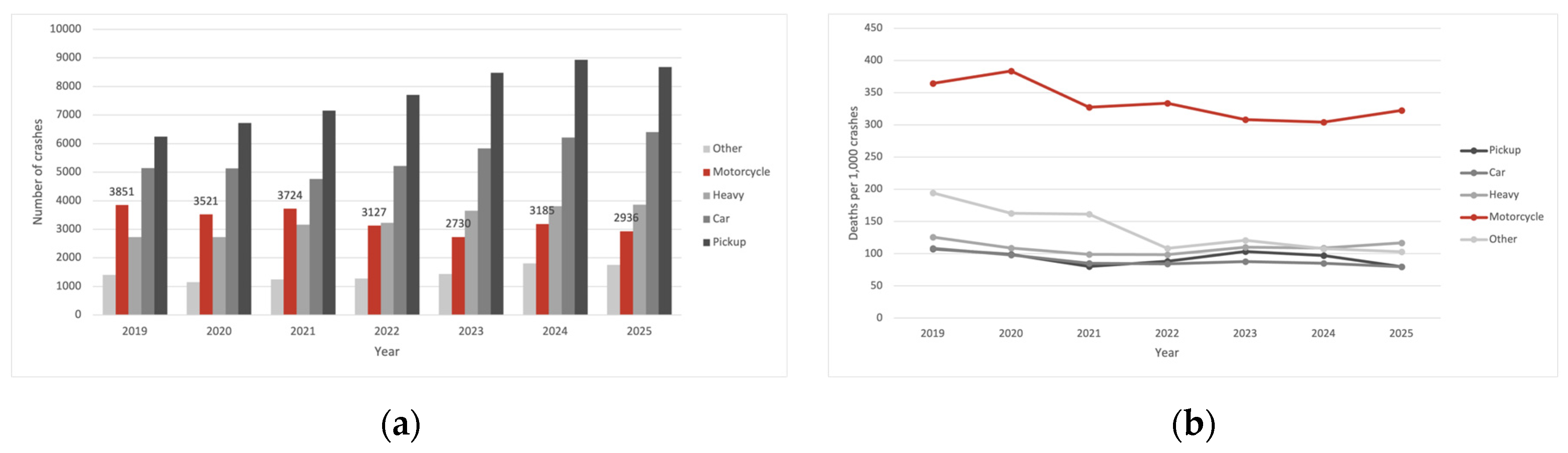
Figure 2.
Sample selection flowchart for the analytical dataset of motorcycle-involved crashes, Thailand 2019–2025.
Figure 2.
Sample selection flowchart for the analytical dataset of motorcycle-involved crashes, Thailand 2019–2025.
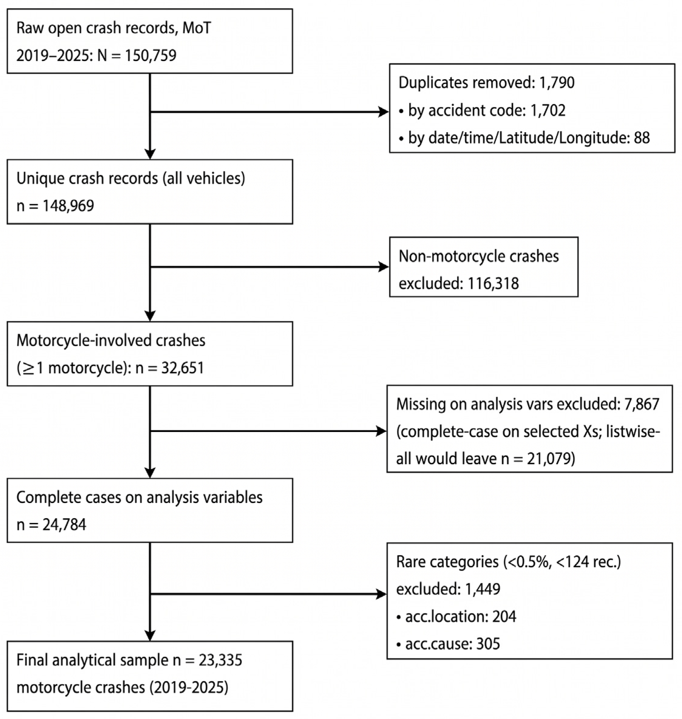
Table 1.
Comparison of representative count-regression studies on crash and fatality severity.
| Author | Response | Covariate | Count Model | Criteria | Main Distinction from the Present Study |
|---|---|---|---|---|---|
| Lord et al. (2010) [23] | Crash counts (underdispersed) at railway–highway crossings, South Korea |
Crossing & traffic characteristics | Poisson, CMP, gamma | Goodness-of-fit comparison |
Applies CMP to underdispersed crash counts at railway crossings, not motorcycle fatalities, and does not model zero inflation or covariate interactions. |
| Khan et al. (2020) [24] | Road traffic accident counts (clustered, longitudinal), Mauritius |
Time-variant explanatory variables (causes of crashes) |
Clustered longitudinal COM-Poisson with gamma random effects (CMP-G) | GQL estimation, comparison with Poisson-gamma & log-normal mixtures | Addresses clustering via random effects rather than a zero-inflation mechanism and does not incorporate location-by-collision-type interactions. |
| Truong & Currie (2019) [25] | Monthly crash count on freeway roadway segments, China | Traffic composition, curve, slope, weather (wind, precipitation, visibility) + interactions | Bayesian spatio-temporal model | Comparison against random effect and spatial models |
Examines roadway-by-weather interaction effects on freeway crash frequency in China using Bayesian spatio-temporal methods but does not address motorcycle-specific fatality severity, zero-inflation, or dispersion-flexible (CMP-family) models. |
| Simmachan et al. (2022) [11] | Fatalities per crash (count), Thailand | Road type, weather, light, month | Poisson, CMP, ZIP, ZICMP | AIC, log-likelihood, Pearson χ2, LRT, score test | Applies ZICMP to general road-traffic fatalities rather than motorcycle-specific crashes and specifies covariates additively without interaction terms. |
| Haleem & Hosseinpour (2024) [26] | Commercial motor vehicle (CMV) crashes at signalized/unsignalized intersections, Kentucky |
Intersection design & control |
ZICMP, Zero-Inflated Hurdle-Truncated CMP (ZI-HTCMP) | AIC, GOF | Focuses on commercial-vehicle intersection crashes rather than motorcycles specifically and does not test whether collision-type lethality varies by location. |
| Banerjee et al. (2025) [27] | Fatal-and-injury distraction crashes at ramp terminals, Kentucky | Ramp-terminal design & control | ZINB, ZICMP, ZIHTCMP (ZIHTCMP best-fitting) | AIC, GOF | Examines distraction- related crashes at ramp terminals with zero-inflated models but does not address motorcycle fatalities or interaction effects between risk factors. |
| Boonkrong & Simmachan (2026) [12] | Road traffic fatalities per accident (count, 0–4), Thailand | Road, region, vehicle, crash type, cause, weather, time | Poisson, NB, ZIP, ZINB, Hurdle Poisson, Hurdle NB | AIC, BIC, χ2, pseudo-R2, MAE, RMSE, Friedman, Vuong, 5-fold CV | Compares a broad set of count models for general road-traffic fatalities across all vehicle types but does not isolate motorcycles or test covariate interactions. |
| Pathivada et al. (2025) [28] | Motorcycle crash frequency on rural multilane segments, Kentucky | AADT, shoulder width, horizontal curves, undivided alignments, cable median barrier |
CMP, Heterogeneous CMP (HTCMP) | GOF screening, out-of-sample validation (MAD, MSPE), empirical Bayes ranking |
Applies CMP-family models to motorcycle crash frequency along corridors, not fatality severity per crash, and does not incorporate zero inflation or interaction terms. |
| Present study | Deaths per motorcycle crash (count), Thailand | Crash type, location, cause, weather, year, month, time + interactions | Poisson, CMP, ZIP, ZICMP (+interaction) | LRT, AIC, BIC, score test | — |
Note. GOF = goodness-of-fit; GQL = generalised quasi-likelihood; CMP-G = Conway–Maxwell–Poisson with gamma random effects; ZI-HTCMP = zero-inflated heterogeneous Conway–Maxwell–Poisson; LRT = likelihood-ratio test; AIC = Akaike Information Criterion; BIC = Bayesian Information Criterion. Studies are ordered by publication year. Dashes (—) indicate not applicable.
Table 2.
Descriptive statistics and fatality severity by covariate (n = 23,335).
| Category | n | % | Mean Deaths/Crash | % Fatal (≥1) |
|---|---|---|---|---|
| Collision type | ||||
| Rear-end (ref) | 14,240 | 61.02 | 0.285 | 25.3 |
| Run-off-road crash | 4612 | 19.76 | 0.350 | 32.7 |
| Head-on | 2309 | 9.89 | 0.577 | 47.5 |
| Collision with fixed object | 1775 | 7.61 | 0.435 | 38.4 |
| Pedestrian-involved | 213 | 0.91 | 0.357 | 31.9 |
| Angle | 186 | 0.80 | 0.403 | 34.4 |
| Accident location | ||||
| Straight (ref) | 19,569 | 83.86 | 0.331 | 29.5 |
| Curve | 2053 | 8.80 | 0.437 | 37.2 |
| Intersection | 882 | 3.78 | 0.319 | 28.1 |
| Access point | 831 | 3.56 | 0.320 | 28.6 |
| Accident cause | ||||
| Human speeding (ref) | 16,057 | 68.81 | 0.347 | 31.0 |
| Environment/animals | 4806 | 20.60 | 0.296 | 26.3 |
| Human impairment | 969 | 4.15 | 0.353 | 28.3 |
| Human non-compliance with signs | 615 | 2.64 | 0.392 | 34.5 |
| Human overtaking | 520 | 2.23 | 0.454 | 37.7 |
| Vehicle defect | 135 | 0.58 | 0.385 | 30.4 |
| Human inexperience | 123 | 0.53 | 0.268 | 25.2 |
| Roadway fixed object | 110 | 0.47 | 0.182 | 16.4 |
| Weather | ||||
| Normal (ref) | 22,174 | 95.03 | 0.335 | 29.7 |
| Adverse weather | 1022 | 4.38 | 0.439 | 38.6 |
| Poor visibility | 139 | 0.60 | 0.309 | 24.5 |
| Time | ||||
| Day (ref) | 15,517 | 66.50 | 0.285 | 25.3 |
| Night | 7818 | 33.50 | 0.448 | 39.6 |
| Year | ||||
| 2019 (ref) | 3628 | 15.55 | 0.359 | 31.2 |
| 2020 | 3406 | 14.60 | 0.340 | 30.1 |
| 2021 | 3244 | 13.90 | 0.328 | 29.5 |
| 2022 | 2953 | 12.66 | 0.334 | 29.8 |
| 2023 | 3434 | 14.72 | 0.349 | 30.6 |
| 2024 | 3445 | 14.76 | 0.330 | 29.5 |
| 2025 | 3225 | 13.82 | 0.334 | 29.6 |
| Month | ||||
| January (ref) | 3209 | 13.75 | 0.280 | 25.2 |
| February | 1574 | 6.75 | 0.376 | 33.0 |
| March | 1629 | 6.98 | 0.371 | 32.8 |
| April | 3798 | 16.28 | 0.247 | 22.4 |
| May | 1328 | 5.69 | 0.406 | 35.2 |
| June | 1260 | 5.40 | 0.421 | 36.9 |
| July | 1443 | 6.18 | 0.404 | 35.8 |
| August | 1265 | 5.42 | 0.403 | 35.1 |
| September | 1335 | 5.72 | 0.369 | 33.3 |
| October | 1451 | 6.22 | 0.416 | 36.2 |
| November | 1668 | 7.15 | 0.421 | 36.6 |
| December | 3375 | 14.46 | 0.276 | 24.7 |
Note. n = number of crashes in category; % = percentage of the 23,335-crash analytical sample; % fatal (≥1) = percentage of crashes in the category with at least one fatality. Reference (ref) categories were set as the most frequent level within each covariate. Percentages within each covariate sum to 100%, subject to rounding. The near-identical severity statistics for the rear-end collision type and the Day time-of-day category are not coincidental: the two categories substantially overlap, with 72.4% of rear-end collisions occurring during daytime and 66.4% of daytime crashes being rear-end collisions.
Table 3.
Comparison of model performance for predicting motorcycle fatality counts (n = 23,335).
| Model | Log-Likelihood | k | AIC | BIC |
|---|---|---|---|---|
| Poisson | −16,836.24 | 39 | 33,750.48 | 34,064.73 |
| CMP | −16,749.85 | 40 | 33,579.70 | 33,902.01 |
| ZIP | −16,667.23 | 52 | 33,438.46 | 33,857.46 |
| ZICMP | −16,417.35 | 53 | 32,940.71 | 33,367.76 |
Note. k = number of estimated parameters, including the intercept; AIC = Akaike Information Criterion; BIC = Bayesian Information Criterion. Lower AIC/BIC values indicate a preferable balance between goodness of fit and model parsimony. The best-fitting model on each criterion is shown in bold.
Table 4.
ZICMP regression estimates for crash-level covariates, excluding interaction terms (n = 23,335).
Table 4.
ZICMP regression estimates for crash-level covariates, excluding interaction terms (n = 23,335).
| (a) Count component | ||||
| Predictor | β | SE |
IRR [95% CI] |
p |
| Intercept | −0.3902 | 0.0638 | 0.68 [0.60, 0.77] |
<0.001 |
| Collision type | ||||
| Angle (ref Rear-end) | −1.1636 | 1.0278 | 0.31 [0.04, 2.34] |
0.258 |
| Fixed-object collision | 0.5263 | 0.0613 | 1.69 [1.50, 1.91] |
<0.001 |
| Head-on | 1.0176 | 0.0564 | 2.77 [2.48, 3.09] |
<0.001 |
| Pedestrian-involved | 0.2639 | 0.1612 | 1.30 [0.95, 1.79] |
0.102 |
| Run-off-road | 0.1449 | 0.0433 | 1.16 [1.06, 1.26] |
<0.001 |
| Accident location | ||||
| Access point (ref Straight) | 0.0762 | 0.1115 | 1.08 [0.87, 1.34] |
0.495 |
| Curve | 0.1914 | 0.0871 | 1.21 [1.02, 1.44] |
0.028 |
| Intersection | −0.0763 | 0.1104 | 0.93 [0.75, 1.15] |
0.489 |
| Accident cause | ||||
| Environment/animals (ref Speeding) |
−0.1343 | 0.0411 | 0.87 [0.81, 0.95] |
0.001 |
| Human impairment | −0.0216 | 0.0757 | 0.98 [0.84, 1.14] |
0.775 |
| Human inexperience | −0.3806 | 0.2189 | 0.68 [0.45, 1.05] |
0.082 |
| Non-compliance with signs | −0.0240 | 0.0941 | 0.98 [0.81, 1.17] |
0.799 |
| Human overtaking | 0.0926 | 0.0983 | 1.10 [0.90, 1.33] |
0.346 |
| Roadway fixed object | −1.1041 | 0.2599 | 0.33 [0.20, 0.55] |
<0.001 |
| Vehicle defect | 0.1194 | 0.1862 | 1.13 [0.78, 1.62] |
0.522 |
| Weather | ||||
| Adverse weather (ref Normal) |
0.1618 | 0.0642 | 1.18 [1.04, 1.33] |
0.012 |
| Poor visibility | −0.3233 | 0.1865 | 0.72 [0.50, 1.04] |
0.083 |
| Year | ||||
| Year 2020 (ref 2019) | −0.2172 | 0.0543 | 0.80 [0.72, 0.90] |
<0.001 |
| Year 2021 | −0.1518 | 0.0549 | 0.86 [0.77, 0.96] |
0.006 |
| Year 2022 | −0.1588 | 0.0560 | 0.85 [0.76, 0.95] |
0.005 |
| Year 2023 | −0.0841 | 0.0531 | 0.92 [0.83, 1.02] |
0.113 |
| Year 2024 | −0.1696 | 0.0540 | 0.84 [0.76, 0.94] |
0.002 |
| Year 2025 | −0.1454 | 0.0550 | 0.86 [0.78, 0.96] |
0.008 |
| (b) Zero-inflation component | ||||
| Predictor | β | SE |
OR [95% CI] |
p |
| Intercept | 0.1018 | 0.0916 | 1.11 [0.93, 1.32] |
0.267 |
| February (ref January) | −0.6716 | 0.1502 | 0.51 [0.38, 0.69] |
<0.001 |
| March | −0.7528 | 0.1537 | 0.47 [0.35, 0.64] |
<0.001 |
| April | 0.3061 | 0.0992 | 1.36 [1.12, 1.65] |
0.002 |
| May | −1.0358 | 0.1867 | 0.35 [0.25, 0.51] |
<0.001 |
| June | −1.2502 | 0.2150 | 0.29 [0.19, 0.44] |
<0.001 |
| July | −1.1641 | 0.1971 | 0.31 [0.21, 0.46] |
<0.001 |
| August | −0.9646 | 0.1868 | 0.38 [0.26, 0.55] |
<0.001 |
| September | −0.7901 | 0.1707 | 0.45 [0.32, 0.63] |
<0.001 |
| October | −1.0115 | 0.1757 | 0.36 [0.26, 0.51] |
<0.001 |
| November | −1.1298 | 0.1761 | 0.32 [0.23, 0.46] |
<0.001 |
| December | 0.0938 | 0.1030 | 1.10 [0.90, 1.34] |
0.362 |
| Night (ref Day) | −1.4703 | 0.1226 | 0.23 [0.18, 0.29] |
<0.001 |
Note. IRR = incidence rate ratio (count component, panel a); OR = odds ratio (zero-inflation component, panel b); CI = confidence interval. Reference (ref) categories are indicated in parentheses. The estimated dispersion parameter was 2.54 (SE = 0.0873), confirming underdispersion (ν > 1). Location-by-collision-type interaction terms, included in the fitted model, are presented separately in Table 5.
Disclaimer/Publisher’s Note: The statements, opinions and data contained in all publications are solely those of the individual author(s) and contributor(s) and not of MDPI and/or the editor(s). MDPI and/or the editor(s) disclaim responsibility for any injury to people or property resulting from any ideas, methods, instructions or products referred to in the content. |
© 2026 by the authors. Licensee MDPI, Basel, Switzerland. This article is an open access article distributed under the terms and conditions of the Creative Commons Attribution (CC BY) license (http://creativecommons.org/licenses/by/4.0/).
Copyright: This open access article is published under a Creative Commons CC BY 4.0 license, which permit the free download, distribution, and reuse, provided that the author and preprint are cited in any reuse.