
Submitted:
02 October 2026
Posted:
06 October 2026
You are already at the latest version
Abstract
Dissective analysis of predictive skill for medium range ensemble streamflow forecasting is carried out for 43 headwater locations in the US. To assess the component-specific contributions of the full HEFS, 20-yr hindcasting experiments were performed for the wettest 3-month period for each location. The results show that, when all ranges of observed flow are considered, hydrologic modeling, the use of NWP precipitation forecast and its post processing, streamflow assimilation and streamflow post processing contribute on average 6, 43, 31 and 20% to the collective predictive skill in reference to climatology, respectively. The contributions vary greatly from location to location and with the magnitude of the verifying observed flow in reflection of the predictability of precipitation and streamflow. When only high flows are considered, the use of NWP precipitation forecast and its post processing is by far the largest contributor. For several locations, including some with significant snowmelt, the predictive skill is noticeably poor due to deficient or very challenging hydrologic modeling relative to climatology. Overall, the results indicate that, for holistic improvement of medium range ensemble streamflow forecasting, efforts should be directed at improving hydrologic modeling particularly at skill-challenged locations in addition to improving future forcings particularly for large events.
Keywords:
ensemble streamflow forecasting
; hydrologic ensemble forecast service (HEFS)
; predictive skill dissection
; data assimilation
; statistical post-processing
1. Introduction
Improving streamflow forecasting entails reducing total uncertainty in streamflow prediction such that the forecast accuracy is increased while the forecast attributes meet the needs of the user decision making and support. In such efforts, headwater basins are of particular interest as they are generally the largest source of uncertainty. Total uncertainty at headwater locations comprises future input uncertainty and hydrologic uncertainty (Krzysztofowicz 1999, WMO 2025). Future input uncertainty refers to the uncertainty in the future forcings such as precipitation and temperature used as input to the hydrologic models. Hydrologic uncertainty refers to structural, parametric and initial condition (IC) uncertainties in the hydrologic and water management models used as well as anthropogenic uncertainties associated with unknown or partially known human control and alterations of movement and storage of water. Accordingly, streamflow forecast systems and processes include components and elements that are aimed at reducing the above uncertainties individually or collectively (Demargne et al. 2014, Troin et al. 2021).
Ensemble forecasts aim at describing higher-order statistical moments of the predictands beyond central tendency while maximizing predictive skill. Because generating such forecasts requires dynamical-statistical coherence, ensemble forecasting lends itself to holistic design, assessment and improvement of the forecast systems and processes. To that end, the Hydrologic Ensemble Forecast Service (HEFS, Demargne et al. 2014; see Figure 1) of the US National Weather Service (NWS) was designed to address input uncertainty with the Meteorological Forecast Ensemble Processor (MEFP, Schaake et al. 2007, Wu et al. 2011, NWS 2019ab), the IC uncertainty with data assimilation (DA) (NWS 2010) and other hydrologic uncertainties with streamflow post processing (Seo et al. 2006, Alizadeh et al. 2020). To date, however, only the MEFP has been implemented across all River Forecast Centers (RFC), leaving large room for potential improvement (Kim and Seo 2025ab).
An important consideration in the design and implementation of an ensemble streamflow forecast system is the availability and quality of streamflow assimilation. Of all hydrologic uncertainties, only the IC uncertainty is lead time-dependent. Because soil moisture and other state variables are rarely observed at the catchment scale, they are typically inferred from real-time observations of streamflow and forcing variables via hydrologic models. If streamflow assimilation is included in the ensemble forecast system, it may not be necessary to include real-time streamflow observations as a predictor in streamflow post processing. The implication for the HEFS, for example, is that one may use the MEFP or its recent enhancement, the conditional bias penalized regression (CBPR)-aided MEFP (Kim et al. 2025, Kim and Seo 2025a), for streamflow post processing as well. The MEFP combines multiscale probability matching, regression (in normal space), downscaling and the Schaake Shuffle (SS, Clark et al. 2004, Wu et al. 2018) for statistical post processing of precipitation forecasts from numerical weather prediction (NWP) models. The CBPR-aided MEFP uses CBPR in place of ordinary least squares regression (OLSR) to ameliorate under-forecasting of heavy-to-extreme precipitation by reducing Type II error (i.e., false negative) for large events but at some expense of increasing Type I error (i.e., false positive) for small events. The use of a common post processing method for both precipitation and streamflow would not only simplify and streamline statistical modeling but may also improve parsimony for reduced data requirements.
With the above backdrop, this paper aims at addressing two objectives. The first is to describe the full HEFS in which streamflow assimilation and streamflow post processing operate in tandem as designed at inception (see Figure 1). The second is to dissect the performance of the full HEFS toward maximizing the collective predictive skill for medium range (~14 days) ensemble streamflow forecasting. A similar study has recently been reported by Zhang et al. (2025) for prediction of mean daily flow at the outlet of the 15,876 km2 upper Huai River Basin in east China using the ensemble Kalman filter for streamflow assimilation, Bayesian Joint Probability method for post processing of precipitation forecast, and Quantile Regression for post processing of streamflow forecast. This study differs significantly from the above in two important ways. First, the spatial scale of the catchments of interest is much smaller in this work, ranging from 190 to 2,400 km2 with a median of 985 km2. In addition, the predictand of primary interest is instantaneous discharge at a 6-hr timestep in line with the operational practices at the RFCs. Second, the relatively small space-time scale associated with the predictands of precipitation and streamflow means that predictability is rather limited (Kim et al. 2025, Kim and Seo 2026), and that Type II error is also an important source of uncertainty particularly for all-important heavy precipitation and high flows (WMO 2025). Accordingly, we use the CBPR-aided MEFP for post processing of precipitation forecasts from NWP and DA-aided streamflow predictions, and the fixed-lag smoother application of the adaptive conditional bias-penalized ensemble Kalman filter for streamflow assimilation (AEnKF, Shen et al. 2022ab, Seo et al. 2022, Kim and Seo 2025b). We then assess the flow magnitude-dependent contributions of hydrologic modeling, NWP precipitation forecast and its post processing, assimilation of streamflow and streamflow post processing to the collective predictive skill of the resulting ensemble streamflow forecast in reference to climatological ensemble streamflow forecast.
This work advances assessment and understanding of the performance of a full ensemble streamflow forecast system for headwater basins and the contribution of each component to the collective predictive skill in short to medium ranges. Whereas the details are given in the context of the HEFS, the general approach and methodology apply to similar ensemble streamflow forecast systems that partition input and hydrologic uncertainties. This paper is organized as follows. Section 2 describes the study locations, data, models and tools used. Section 3 describes the methodological framework, the simplified streamflow post processor and the evaluation approach. Section 4 presents the results and discussions. Section 5 provides conclusions and future research recommendations.
2. Study Locations, Data, Models and Tools Used
The study area comprises 43 headwater locations in the HEFS Testbed (Lee et al. 2018, 2020) in the service areas of 11 RFCs (see Figure 2 for the map and Supplementary Data (SD) 1 for geographical names and hydrologic attributes). In Figure 2, the forecast points are identified by their 5-character NWS abbreviations. The same locations were used in Kim and Seo (2025a) from which 20-yr ensemble precipitation hindcasts covering 2000 to 2019 are available from the NWS Office of Hydrologic Prediction (OWP). The precipitation hindcasts were generated with the CBPR-aided MEFP forced by the Global Ensemble Forecast System Version 12 (GEFSv12) ensemble mean precipitation hindcasts (Guan et al. 2022, Hamill et al. 2022). The observed mean areal precipitation (MAP) and mean areal temperature (MAT) data are from the RFCs. Climatological mean areal potential evapotranspiration (MAPE) is used for both observed and future MAPE. The observed instantaneous streamflow data are from the US Geological Survey.
The hydrologic models used are SNOW-17 for snowmelt (Anderson 1976), Sacramento for soil moisture accounting (SAC, Burnash et al. 1973) and unit hydrograph for surface runoff routing (UHG, Chow et al. 1988). All models are run at a 6-hr timestep even though some RFCs use shorter timesteps for fast-responding basins. The use of the same timestep for all locations is to allow skill assessment under the same hydrologic assimilation cycle of 6 hours. The data assimilated into SAC and UHG include streamflow, MAP and MAPE where MAP comprises rainfall and snowmelt. For SNOW-17, no DA was performed. Hence, the snow model states, including the snow water equivalent (SWE), are not updated throughout the 20-yr hindcast period which may degrade the quality of snowmelt prediction relative to that attainable operationally via manual DA. To counter the potential degradation of MAP due to lack of snow DA, we assumed clairvoyant future temperature in this work by using MAT in place of temperature forecast. Franz et al. (2014) reports that, for water supply forecasting, the impact of SWE DA relative to DA-less prediction is mixed; whereas DA improved percent bias for ensemble mean forecasts, ensemble forecasts were more skillful without DA. The above finding suggests that the combination of no snow DA and clairvoyant temperature forecast likely inflates the accuracy of snowmelt prediction. Whereas the assumption of clairvoyant temperature forecast is an apparent limitation of this study, it avoids potentially under-representing the predictive skill attainable in the current operations at the RFCs, which is generally not reproducible, and has little impact on the principal findings of this work as shown in the Results and Discussions Section. For medium range streamflow forecasting, SWE and streamflow should ideally be assimilated jointly as a coupled inverse problem. Such coupled DA and the use of temperature forecast warrant separate attention and is left as a future endeavor. Figure 3 describes the dataflow for the hindcast experiment.
Reducing hydrologic uncertainty necessarily depends on the quality of hydrologic modeling, including that of observed forcings. Significant but easily addressable biases or systematic errors in observed forcings or hydrologic model parameters likely inflate the impact of streamflow assimilation and post processing whereas poorly modeled UHG likely deflates the impact of streamflow assimilation (Kim and Seo 2025b). For critical assessment of predictive skill of an ensemble streamflow forecast system, it is hence desirable to reduce such errors as much as possible. To that end, we used AB_OPT (Adjoint-Based OPTimizer, Seo et al. 2009) to correct long-term biases in MAP and MAPE, refine the operational UHG (or newly estimate if necessary) and locally optimize the SAC parameters using the operational settings as starting points. AB_OPT uses adjoint-based optimization to estimate the biases and UHG and the Sequential Line Search (SLS, Kuzmin et al. 2008) to refine the SAC parameters. For the majority of the locations, the magnitude of the adjustment and refinement is relatively small. For some locations, however, the adjustment is rather significant, particularly for UHG due to flow magnitude-dependent variations. Figure 3 shows how AB_OPT was used for the hindcast experiment in this work.
3. Methodology
Ensemble forecasting is a form of Monte Carlo integration for the predictive conditional probability density function (PDF) sought. Hence, an ensemble streamflow forecast system and its composition are determined by this PDF as described below for the HEFS and similar systems.
3.1. Ensemble Streamflow Prediction
For medium range ensemble streamflow forecasting, The HEFS numerically derives the conditional PDF of streamflow valid up to 14 days into the future, given the observed streamflow valid up to and including the current time and the GEFS ensemble mean forecasts of precipitation and temperature valid at the same future times. The above PDF may be written as where qf is the future streamflow, qo is the observed streamflow and is the ensemble mean forecasts of precipitation and temperature. Throughout this paper, f( ) denotes a PDF in which only the experimental values of the random variables are indicated for brevity. For example, abbreviates where Qf, Qo and are the random variables, and qf, qo and are their experimental values, respectively. In some forecast systems, the predictor for the forcings may be ensemble forecasts from NWP, pf, rather than their ensemble mean, , or some other single-valued representation. In such cases, pf would replace with little loss of generality. One may of course choose to model purely statistically or exclusively via machine learning, but most operational agencies use hydrologic modeling to leverage encapsulated knowledge (Abbott 1999).
Introducing the hydrologic model-predicted streamflow valid at the same future times, sf, the above conditional PDF may be written via the total probability law as (Krzysztofowicz 1999, Seo et al. 2006):
where sf is the future streamflow due to the future forcings and the ICs of the hydrologic models. In the above, may be written in terms of the uncertainty sources modeled:
where bf is the future input forcings and ic is the ICs of the hydrologic models. Inserting Eq. (2) into Eq. (1), we have for :
Noting that Bf is independent of Qo and the ICs are independent of future forcings, one may reduce and to and f5(ic| qo), respectively. Similarly, noting that ic and bf in reflect qo and via f5(ic| qo) and , respectively, one may reduce to f4(sf| bf,ic). Because sf already reflects qo and via in Eq. (1), one may reduce to f2(qf| sf). With the above reductions, Eq. (3) may be rewritten as:
Eq. (4) captures the 4 scientific components of the full HEFS where f2(qf| sf), f4(sf| bf,ic), f5(ic| qo) and represent streamflow post processing, hydrologic modeling, streamflow assimilation and future input uncertainty processing, respectively (see Figure 1). In most operational practices, hydrologic models do not include uncertainty terms. Hence, f4(sf| bf,ic) is an impulse function which simply maps ic and bf to sf with a probability of unity. Figure 4 depicts the ensemble generation process associated with Eq. (4) where the order of f5(ic| qo) and may be reversed with no loss of generality. If desired, one may include parametric uncertainty or multi-model ensembles in the above. Because a unique combination of a hydrologic model and a parameter set defines a unique state space, multi-model ensembles are algorithmically no different from multi-parameter ensembles. In this work, parametric uncertainty or multi-model ensembles are not considered because such processing is unlikely to be operationalized in the very near future due to the computational cost associated with performing DA for each state space and the challenges associates with modeling parametric uncertainty and its interpretation by human forecasters.
Hydrologic modeling is described in Section 2, the MEFP is described in Schaake et al. (2007), Wu et al. (2011) and NWS (2019ab), the CBPR-aided MFEP is described in Kim et al. (2025) and Kim and Seo (2025a) and streamflow assimilation is described in Shen et al. (2022ab), Seo et al. (2022) and Kim and Seo (2025b). Streamflow assimilation is applied in a strongly-constrained mode in this work, i.e., the hydrologic models act as equality constraints in the optimization. Hence, the DA results reflect, and often reveal, deficiencies in hydrologic modeling which may be difficult to detect and identify in forward simulations alone (Lee et al. 2019, Kim and Seo 2026). Below, we describe post processing of DA-aided streamflow predictions via the CBPR-aided MEFP.
3.2. Post Processing of DA-Aided Streamflow Predictions
Streamflow post processing addresses hydrologic uncertainty only. Hence, one may exclude future input uncertainty by replacing the forecast forcings in Eq. (4) with the observed forcings which are assumed uncertainty-free over the prediction horizon:
SD 2 shows the numerical integration of Eq. (5) and hence the ensemble generation process for parameter estimation and verification of streamflow post processing. A practical challenge in modeling the streamflow post processor, f2(qf| sf) in Eq. (5), is that, depending on the relative proximity of the ensemble members to the (unknown) true state in the state space, the predictive skill of sf may vary from one ensemble member of Ic to the next. Hence, it may be necessary for parameter estimation of , where ni is the ensemble size for streamflow assimilation (see Figure 4), to be ensemble member-specific, making it computationally very expensive. Alternatively, one may assume that the predictive skill of ensemble mean of sf, or , is comparable to that of , and approximate Eq. (5) with:
In other words, collapse the ensemble members of Sf, , into ensemble mean of Sf, , and use it as the sole predictor in streamflow post processing, thereby reducing computational cost for parameter estimation by a factor of ni. The above simplification does not mean that the DA-updated uncertainty in the ICs is ignored. Rather, the updated IC uncertainty is lumped together with all other hydrologic uncertainties into . In this work, a single set of hydrologic models (i.e., SNOW-17, SAC and UHG) and a single set of model parameters are used. Hence, one may expect the ensemble members, , to be strongly inter-correlated and most of the information content therein to be explainable by a very small number of orthogonal components (Brown and Seo 2009). In such a case, one may expect Eq. (6) to be a good approximation of Eq. (5). Indeed, limited comparative analysis indicates that the impact of the simplification is negligible. If multiple models or multiple sets of model parameters are used, however, Eq. (6) is not likely to be reasonable. SD 2 shows the ensemble generation processes under the above simplification which is to be compared with Figure 4.
When represented by in Eq. (6), post processing of streamflow is completely analogous to that of precipitation forecast represented by in Eq. (4). Hence, in principle, one may use the CBPR-aided MEFP not only for precipitation but also for streamflow. The MEFP combines multiscale probability matching for bias correction, linear regression in normal space for statistical prediction, multiscale downscaling via historical ensemble traces and the SS to stitch together the synthetic ensemble traces across different canonical events (CE) while preserving rank correlation in the historical ensemble traces. Contrary to the name, CEs are not events in the hydrometeorological or probabilistic sense but forecast sub-horizons of varying durations and hence equivalent to support in geostatistics. To apply the CBPR-aided MEFP to streamflow post processing, however, a few modifications are desirable as elaborated below.
The first pertains to distribution modeling. In the CBPR-aided MEFP, and the verifying observed precipitation are assumed to follow 2-parameter Weibull or gamma distributions (NWS 2019ab). In streamflow post processing, empirical distributions are used instead. Streamflow is strongly modulated by regime-dependent hydrologic processes, fixed boundary conditions across scale and anthropogenic controls and alterations by varying degrees. Hence, the probability distribution of streamflow varies very widely and, unlike precipitation, is often not well described by additive or multiplicative random processes which lead to known parametric distributions (Benjamin and Cornell 2014). The use of empirical distributions means that it is necessary to model the tails outside of the historically observed ranges. The left tail is of little practical concern because the magnitude of flow involved is very small though it may significantly impact certain verification statistics such as the rank histogram. The right tail, on the other hand, has large impact on large to extreme flows, including record-breaking flows, and hence requires care. In this work, we use the hyperbolic model for the right tail end (Deutsch and Journel 1998):
In the above, Q is instantaneous flow (observed or simulated), FQ≥(q) is the cumulative distribution of Q, qmax is the maximum observed or predicted flow, pmax is the probability of less than or equal to qmax and is the user-specified parameter which controls the length of the tail (the smaller, the longer). In this work, we used = 3.25 for all locations based on limited sensitivity analysis.
The second modification pertains to the modeling of temporal variability of the ensemble traces over the forecast horizon sampled from in Eq. (6). Compared to the modeling of probability distribution or conditional bias, temporal variability modeling is of second-order importance (Wu et al. 2018). The quality of temporal variability, however, impacts the quality of multi-daily flow forecasts and hence is likely important for large events. In the MEFP and CBPR-aided MEFP, the SS matches rank correlation of the ensemble traces sampled from to that of the climatological precipitation forecast (for graphical illustration, see Figure 3 of Kim and Seo 2025a). In streamflow post processing, the SS is modified to match rank correlation of the post-processed streamflow prediction to that of the DA-aided. The rationale for the above change is that, for large events, the temporal variability of DA-aided streamflow prediction is likely much more realistic than that of the climatological streamflow forecast. Whereas the DA-aided predictions reflect the current hydrologic and hydrometeorological conditions, climatological streamflow forecasts are bound to include many historical traces of low flow which are overly persistent for large events. Below, we provide a brief algorithmic description of the CBPR-aided MEFP as applied to streamflow post processing after Kim and Seo (2025a).
Given the DA-aided ensemble mean streamflow forecast, , the streamflow post processor samples synthetic traces from for each CE where is modeled using CBPR (Kim et al. 2025). Figure 5 shows the 77 CEs used for streamflow post processing. Though not pursued in this work, the CE selection may be empirically optimized to maximize skill while minimizing the number of CEs used (see Kim 2024 for an example for precipitation). The streamflow post processor then uses the SS to stitch together the CE-specific synthetic traces of streamflow with the temporal variability of the DA-aided ensemble streamflow forecast in the ordinal sense over the forecast horizon of 14 days. The SS starts with the DA-aided ensemble streamflow forecast at a 6-hr timestep valid over the forecast horizon. For a given CE, the ensemble members are aggregated to the duration of the CE and sorted in the ascending order. The streamflow post processor samples synthetic traces from the CE-specific and sort them in the ascending order. Each of the sorted, or rank-ordered, synthetic traces is then assigned the ensemble member identifier in which the DA-aided streamflow forecast of the same rank occurred.
For example, if the CE covers 0-to-96 hrs of lead time (see Figure 5) and the largest DA-aided streamflow prediction in this 4-day period occurred in the 21th ensemble member for the basin of interest, the largest synthetic trace sampled from the CE-specific is assigned an ensemble member identifier of “21”. The SS then updates each synthetic trace from the latest shuffling of the ensemble streamflow forecast at a 6-hr timestep (recall that this is initially the DA-aided ensemble streamflow forecast) by multiplicatively adjusting the instantaneous streamflow at a 6-hr timestep uniformly within the CE such that the adjusted mean flow is the same as the synthetic trace sampled from the CE-specific . The above process is repeated for all CEs beginning with the CE with the smallest Pearson product-moment correlation, or correlation for short, in the bivariate standard normal space between the positive DA-aided ensemble mean streamflow forecast and the positive observed streamflow and ending with the CE with the largest correlation.
The above sequence of operations cumulatively reflects the temporal patterns of granularity in instantaneous streamflow at a 6-hr timestep gleaned from the successive adjustments during the SS while utilizing all available scale-dependent skill in the input DA-aided ensemble mean streamflow forecast. Once the above steps are completed for all CEs, one has replaced the initial traces of the DA-aided ensemble streamflow forecast over the forecast horizon with the same number of ensemble traces of post-processed streamflow. The resulting ensemble streamflow forecast reflects the multi-scale predictive skill in the DA-aided ensemble mean streamflow forecast over different parts of the forecast horizon and share the same rank correlation and temporal variability in the ordinal sense.
The conditional distributions of observed flow, Y, given the ensemble mean of DA-aided streamflow prediction, X, is modelled identically to that of observed precipitation given the ensemble mean precipitation forecast as described in Wu et al. (2011). The only algorithmic difference is that Pr[Y = 0| X = x,X > 0], denoted as c(x) in Wu et al. (2011), is evaluated empirically in this work rather than analytically due to the use of empirical cumulative distribution functions for positive X and Y. For ephemeral basins, intermittency in streamflow is modeled in the same way as precipitation intermittency (Wu et al. 2011).
Lastly, in streamflow post processing, the CBPR coefficient is estimated without magnitude-dependent optimization (Kim et al. 2025), i.e., by minimizing mean CRPS only once using all available pairs of positive DA-aided prediction and verifying observed flow. In magnitude-dependent optimization, the number of pairs of positive observed flow and positive DA-predicted flow are successively reduced by incrementally increasing the conditioning threshold. The rationale for this simplification is that, unlike precipitation forecasts, magnitude-dependent biases in streamflow prediction tend to arise from regime-dependent errors or routing errors. In such cases, the CBPR coefficient from magnitude-dependent optimization likely lacks robustness necessary for use in operational forecasting.
3.3. Evaluation
Eq. (4) provides the framework for evaluation as well; using climatological streamflow forecast as reference, evaluate the incremental contributions of hydrologic modeling, f4(sf| bf,ic), the use of NWP precipitation forecast and its post processing, , streamflow assimilation, f5(i| qo), and post processing of the DA-aided streamflow predictions, f2(qf| sf) (or with simplification), to the collective predictive skill. Climatological streamflow forecast, or climatology for short, is constructed by sampling observed streamflow over the same prediction horizon of 14 days as the subject forecast from each of the available historical years except the year of the hindcast. Due to many missing streamflow observations, the ensemble size for climatology varies from location to location and from one prediction time to another. The minimum ensemble size used for climatology is 10 to include as many locations as possible.
The primary measure used to assess the predictive skill of the subject forecast in reference to climatology is the CRPSS. The CRPSS is equivalent to the percent reduction in mean CRPS by the subject forecast over the reference forecast:
where and are the mean CRPS (Hersbach 2000) of the reference and subject forecasts, respectively. The CRPS is a continuous integration of the Brier Score (BS, Brier 1951) weighted by the magnitude of the predictand. Hence, mean CRPS reflects reliability, resolution and uncertainty via the calibration-refinement decomposition of the BS and Type II conditional bias, discrimination and sharpness via the likelihood base rate decomposition (Murphy and Wrinkler 1987). Because reliability and Type II conditional bias are competing attributes over the tails of the distribution, it is necessary to assess at minimum reliability and Type II conditional bias or, alternatively, discrimination (WMO 2025). In this work, we assess reliability using the reliability diagram and discrimination using the relative operating characteristic (ROC) which is insensitive to reliability (WMO 2025).
Large-sample hindcasting of the full HEFS for many locations is expensive. Given that flood and water supply forecasting is often the most important service for the producers of ensemble streamflow forecasts, we limit ourselves to the wettest consecutive 3 months for each location in this work. This means that the predictive skill for the entire year is likely larger than that seen in this work. Comparative verification of the MEFP and CBPR-aided MEFP using 20-yr precipitation hindcasts has shown that 10-fold cross validation results are very similar to the dependent validation results (Kim and Seo 2025a). This is an indication that parametric uncertainty due to interannual variability of precipitation is relatively small for the CBPR-aided MEFP owing to the parsimony of the statistical modeling. Accordingly, we used the 20-yr precipitation ensemble hindcasts generated with the CBPR-aided MEFP in a dependent validation mode in this work available from the NWS OWP. For streamflow post processing, 2-parameter Weibull and gamma distributions are replaced by a combination of empirical distributions and hyperbolic modeling of the upper tail as described above. Hence, streamflow post processing is likely subject to larger sampling uncertainties than precipitation post processing. For this reason, we carried out leave-one-year-out cross validation for streamflow post processing.
3.4. Results and Discussion
Before presenting the results for dissection of predictive skill, we first assess the performance of the streamflow post processor described above under clairvoyant input forcings. In this way, we may validate its performance without being obscured by future input uncertainty. The following questions are to be addressed. Does the streamflow post processor consistently improve accuracy over streamflow assimilation alone? How significant is the margin of improvement? Are the post-processed streamflow ensembles reliable? How does streamflow post processing impact the discriminatory skill of the DA-aided predictions? What are the factors impacting the performance?
3.5. Assessment of Streamflow Post Processing
Figure 6a shows the CRPSS averaged over all 43 locations vs. lead time of the base (i.e., DA-unaided) prediction, or CRPSSBASE (black), the DA-aided prediction, or CRPSSDA (red), the post-processed DA-aided prediction, or CRPSSPP (blue), and the post-processed DA-aided prediction under perfect weak-sense reliability, or (purple), for all ranges of observed flow. The reference forecast is climatology. The number parenthesized in the title of each panel indicates the number of locations included. For base and DA-aided predictions, the hydrologic models are initialized with warm states generated by running the models with observed forcings over the entire period of record prior to hindcasting. For the base prediction, the warm states are perturbed based on the observational uncertainties for MAP and MAPE over the assimilation window used for DA. For the DA-aided prediction, the perturbed warm states are updated via AEnKF based on the observational uncertainties for MAP, MAPE and streamflow (Kim and Seo 2026). In this way, we do not unfairly penalize the base predictions for lack of hedging vs. the DA-aided predictions. is calculated using the potential mean CRPS, , via the mean CRPS decomposition (Hersbach 2000):
where REL, RES and UNC are reliability, resolution and uncertainty, respectively. Figs 6bcd show the results for verifying observed flow exceeding the 90th, 95th and 99th percentiles, respectively.
The CRPSS results vary greatly from one location to another in reflection of the widely varying hydrologic predictability (Kim and Seo 2026). To provide a sense of the variations across all locations, SD 3 shows the location-specific CRPSS overlaid in single plots where the worst-performing locations for CRPSSBASE are identified by name. Before summarizing the results, two comments are in order. First, the largest conditioning threshold of the 99th percentile is generally much smaller than flood flow. Hence, the 99th percentile results provide only a glimpse into how streamflow post processing might perform for flood flows. Second, the conditional CRPSS shown in Figs 6bcd and SD 3 is not a proper score. If used by itself, such scores will lead to frequent poor decisions. Potential for misinterpretation or misuse, however, may be avoided by accompanying them with the unconditional results such as Figure 6a and the relationship between the two (WMO 2025). For example, one may write mean CRPS as:
E [CRPS] = E[CRPS| obs > qc]Pr[obs > qc] + E[CRPS| obs ≤ qc]Pr[obs ≤ qc]
where obs is the observed flow, qc is the threshold flow of choice and Pr[∙] is the probability of occurrence of the event bracketed. Note in Eq. (10) that Pr[obs > qc] is the familiar exceedance probability. Depending on one’s verification interest, one may use any conditioning event as long as the two conditioning events in Eq. (10) are mutually exclusive and collectively exhaustive.
Figure 6 indicates the following. On average, streamflow post processing improves over streamflow assimilation beyond the first day or so of lead time. Over very short lead times, however, streamflow post processing adds little for most locations. This is because DA-aided predictions are highly accurate where the IC memory is very strong. Statistical correction via post processing, on the other hand, improves accuracy at longer lead times where the IC memory fades and other hydrologic errors take hold. When all ranges of flow are considered, CRPSSPP is very close to (see Figure 6a), an indication that the post-processed streamflow ensembles are generally very reliable in the weak sense. This is because low flows, which dominate the sample size, are highly predictable. For higher flows, however, the post-processed streamflow ensembles are increasingly less reliable as predictability quickly decreases (see Figs 6bcd). Figure 6 also shows that CRPSSBASE for high flows is significantly larger than that for all ranges of flow. This is because hydrologic modeling is generally more skillful for high flows than low flows relative to climatology which is very poor for high flows. The location-specific results (see SD 3) indicate that the impact of streamflow post processing is mostly positive for most locations but the magnitude of the impact varies very significantly from location to location in reflection of the wide variations in hydrologic predictability. The margin of improvement by streamflow DA and streamflow post processing is particularly large for basins where snowmelt is important due to a combination of longer hydrologic memory associated with snowmelt (Kim and Seo 2026) and increased error in streamflow simulation arising from increased error in MAP which comprises rainfall and (DA-unaided) simulated snowmelt.
Climatological streamflow forecast is free from parametric, structural or anthropogenic uncertainties but has fully saturated IC and future input uncertainties. If the hydrologic uncertainty in streamflow prediction under clairvoyant future forcings is larger than the total uncertainty in climatological streamflow forecast, it is a clear indication that hydrologic modeling warrants attention (Kim and Seo 2026). One may identify such locations by examining location-specific CRPSSBASE. SD 3 indicates that MFNW1 and ORTW1 in the NWRFC, GTBM3 in the NERFC and CWAC1 and FTJC1 in the CNRFC are such skill-deficient locations. Scatter plots of the DA-aided predictions vs. observed flow for the above locations (see SD 4) show large variations in the quality of the predictions and pronounced sensitivity to the ICs. SD 4 also illustrates how regime-dependent errors may be particularly challenging for streamflow post processing. The first 3 of the above 5 locations have snow fractions over 20% and the first 2 have glaciers (see SD 1). It is very likely that the uncertainties in snowmelt simulation and the lack of glacier modeling contributed to the deficient skill at these locations. Recall that snowmelt is a part of the observed precipitation input to SAC. Hence, even a small but consistent error in snowmelt simulation may greatly deteriorate skill for streamflow prediction particularly for low flows. In addition, snowmelt is strongly seasonal and often very predictable which makes climatological streamflow forecast highly competitive. For the above locations, hydrologic modeling should ideally be addressed first before streamflow DA and streamflow post processing may be applied.
Figure 7 shows the reliability diagrams of the post-processed DA-aided predictions of instantaneous flow at selected lead times of the first 6-hr period in Day 1, the last 6-hr period in Day 4 and the last 6-hr period in Day 14. The thresholds used are the 50th, 90th, 95th and 99th percentiles of observed flow. In each plot, there are 43 curves corresponding to the 43 locations. Recall that the streamflow post processor samples ensembles from (see Eq. (6)) which is equivalent to the conditional PDF in the calibration-refinement factorization (Murphy and Winkler 1987). Hence, if the assumptions behind the post processor are met, one may expect the post-processed ensemble to be reliable in the strong sense. Figure 7 thus informs how well the assumptions for the multiscale probability matching, regression, downscaling and the SS may be met given the limits of hydrologic predictability.
In Figure 7, the slanted “S” shape in the reliability curves at the shortest lead time is due to heteroscedasticity of the error in the bivariate normal space as explained below. In the MEFP or CBPR-aided MEFP, the predicted flow and the verifying observed flow resulting from normal transformation are assumed to be jointly normal. At very short lead times, the errors in the DA-aided predictions primarily reflect flow-dependent structural and parametric uncertainties particularly when DA is strongly constrained. Such errors tend to vary significantly across different flow regimes in the joint normal space and are often larger over the tails than in the middle of the distribution relative to the ellipsoidal joint normal PDFs. Because the CBPR or OLSR does not model heteroscedasticity, the predicted probability tends to over- and under-prescribe small and large probabilities, resulting in over- and under-spread ensembles in the middle and over the tails of the distribution, respectively. As the lead time increases, the errors become more random and the pattern largely disappears.
Figure 7 indicates that the post-processed streamflow ensembles are generally reliable. The degree of reliability, however, varies significantly from location to location and tends to deteriorate at the lowest and highest thresholds. There are several locations where reliability is noticeably poor. Such results are due primarily to deficient or very challenging hydrologic modeling and cannot, in general, be addressed effectively by streamflow assimilation, which depends on the fidelity of hydrologic modeling, or post processing, which depends on the statistical attributes of the DA-aided predictions. Whereas a more complex streamflow post processor might improve reliability, it is likely to increase the degrees of freedom and hence data requirements for parameter estimation.
Reliability, or Type I conditional bias, competes with Type II conditional bias over the tails of the distribution of the predictand. Recall that AEnKF used for streamflow assimilation addresses Type II error jointly with Type I error. Streamflow post processing without magnitude-dependent optimization of the CBPR coefficient, on the other hand, mainly addresses reliability. Hence, it is necessary to assess the impact of streamflow post processing on the discriminatory skill of the DA-aided predictions. For this purpose, we use the area under the curve (AUC) of the ROC. Figure 8 shows the AUC averaged over all available locations of the base predictions (black), DA-aided predictions (red) and post-processed DA-aided predictions (blue) under clairvoyant future forcings. The conditioning events are the verifying observed instantaneous flow exceeding the 50th, 90th, 95th and 99th percentiles for the respective locations. Note that some locations could not be included at the highest threshold due to lack of data points. Predictions with perfect discrimination have an AUC of unity. Predictions with no discriminatory skill have an AUC of 0.5.
Figure 8 shows that the AUC of the post-processed DA-aided predictions is nearly identical to that of the DA-aided (i.e., red and blue lines overlap), an indication that streamflow post processing has little impact on the discriminatory skill of the DA-aided prediction. This is not very surprising in that streamflow post processing without magnitude-dependent optimization largely functions as a reliability operator, and that ROC, and hence AUC, is insensitive to reliability. Figure 8 shows that streamflow assimilation using AEnKF significantly improves discrimination over the base prediction for all conditioning thresholds owing to the conditional bias-aware assimilation of real-time observations. To provide a sense of the variations across all locations, SD 5 shows the location-specific results overlaid in single plots. Note that some of the reliability-deficient locations in SD 3 reappear in SD 5, but that there are new locations that are deficient in discrimination, i.e., LNDK1 in MBRFC and CATA1 in SERFC. Similarly to the reliability-deficient locations, discrimination-deficient locations indicate regime-dependent errors in the DA-aided predictions (see SD 4). For these locations, hydrologic modeling should be improved first before streamflow assimilation and streamflow post processing may be applied. Collectively, the results presented in this subsection indicate that the streamflow post processor improves accuracy over streamflow assimilation, renders the DA-aided predictions reliable for most locations and retains the discriminatory skill of the DA-aided predictions. For a number of locations, however, performance is noticeably poor due to deficient or very challenging hydrologic modeling.
3.6. Component-Specific Contributions to Predictive Skill
With the performance of the simplified streamflow post processor assessed, we are now in a position to assess the component-specific contributions to the overall predictive skill in reference to climatology. Table 1 summarizes the forecasts assessed.
In Table 1, CLIMP refers to the ensemble streamflow forecast generated by forcing the hydrologic models with climatological ensemble precipitation forecast. The hydrologic models are initialized with warm states generated by running the models with observed forcings over the entire period of record prior to hindcasting. The warm states are perturbed in the same way as described in Section 4.1. Hence CLIMP represents an imperfect translation of climatological forcings to future streamflow using imperfect hydrologic models with skillful initialization and is equivalent to the long-standing NWS operation Ensemble Streamflow Prediction (ESP, Day 1985) but with perturbed ICs. Climatological ensemble streamflow forecast, on the other hand, represents a perfect translation of climatological forcings to future streamflow using perfect hydrologic models but with skill-less ICs. Climatological ensemble precipitation forecast is sampled from each year of the historical record except the year of the hindcast over the same forecast horizon of 14 days as the subject forecast. The forecast GEFS_CM refers to the streamflow prediction forced by the post-processed NWP precipitation forecast where the post processor is the CBPR-aided MEFP and the NWP forecast is the GEFS ensemble mean. The forecast DA refers to the DA-aided streamflow prediction forced by GEFS_CM. The forecast PP refers to the post-processed DA-aided streamflow prediction.
Figure 9a shows the CRPSS of CLIMP (green), GEFS_CM (black), DA (red) and PP (blue) for all ranges of flow vs. lead time averaged over all 43 locations. The gray line, which is to be compared with GEFS_CM (black) only, represents the CRPSS of the DA-less streamflow prediction forced by the ensemble precipitation hindcasts from the MEFP, rather than the CBPR-aided MEFP, with the same GEFS ensemble mean precipitation forecast as input. The CRPSS results vary greatly from location to location in reflection of the widely-varying predictability of precipitation and streamflow. To provide a sense of the variations of the CRPSS, SD 6 shows the location-specific results and identifies skill-deficient locations. It is important to note that the same 5 skill-deficient locations in SD 3 (see Section 5.3), of which 3 have snow fractions over 20%, reappear in SD 6. Recall that SD 3 reflects hydrologic uncertainty only whereas SD 6 reflects both input and hydrologic uncertainties. The above result suggests that, for those basins where snowmelt is important, the hydrologic uncertainty associated with snowmelt modeling is likely a larger modulator of predictive skill seen in Figure 9 than the input uncertainty associated with precipitation and temperature forecasts. The CRPSS of CLIMP at the lead time of 6 hrs closely reflects the skill of DA-unaided streamflow analysis (i.e., streamflow prediction at the lead time of 0 hrs) and hence reflects the quality of hydrologic modeling, including that of observed forcings (Kim and Seo 2026). The CRPSS of CLIMP with perfect hydrologic modeling and perfectly skillful initialization and forcings would be unity whereas that with perfect hydrologic modeling but with skill-less initialization and forcings (such as climatology) would be zero. The asymptotic CRPSS of CLIMP at long lead times also reflects the quality of hydrologic modeling. If hydrologic modeling is perfect, the future forcings are skill-less and the ICs are skillful, the CRPSS of CLIMP would be significantly positive at short lead times and decrease toward zero as the lead time increases. Because hydrologic modeling is never perfect in reality, the CRPSS of CLIMP typically turns negative as the lead time increases by varying margins.
The rate of decay of the CRPSS of CLIMP reflects the hydrologic memory of the catchment for streamflow generation captured by hydrologic modeling. The more slowly or quickly the CRPSS of CLIMP decays with increasing lead time, the longer or shorter hydrologic memory is, respectively, in reflection of the residence time of the streamflow-generating runoff. Hence, one may consider the area between the CRPSS of CLIMP (green) and the line of zero CRPSS as representing the skill due to a combination of hydrologic modeling, initialization and hydrologic memory as represented by the hydrologic models. A negative area due to negative CRPSS contributes negatively. The difference in CRPSS between GEFS_CM and CLIMP (i.e., the area between the black and green lines) represents the skill added by the NWP precipitation forecast and its post processing. The difference in CRPSS between DA and GEFS_CM (i.e., the area between the red and black lines) represents the skill added by streamflow assimilation. The difference in CRPSS between PP and DA (i.e., the area between the blue and red lines) represents the skill added by streamflow post processing.
In Figure 9a, the contributing areas associated with CLIMP, GEFS_CM, DA and PP are 0.22, 1.60, 1.18 and 0.75 (days), respectively. Hence, on average over all 43 locations, the 4 components of f4(sf| bf,ic), , f5(ic| qo) and in Eq. (4) contribute 6.0, 42.6, 31.5 and 19.9% to the collective predictive skill, respectively, when all ranges of flow are considered. The rather low contribution by f4(sf| bf,ic) is due to the fact that its CRPSS usually falls below zero at large lead times which contributes negatively. Figs 9bcd shows the results for observed flow exceeding the 90, 95th and 99th percentiles, respectively. It is immediately clear that the conditional results of Figs 9bcd are very different from the unconditional results of Figure 9a. For verifying observed flow exceeding the 99th percentile, streamflow post processing contributes little and the contribution of streamflow DA is significant only over the first two days or so of lead time where the IC memory is strong. For Figure 9d, the contributing areas associated with CLIMP, GEFS_CM, DA and PP are 0.58, 3.32, 0.30 and 0.01 (days), respectively, and the 4 components of f4(sf| bf,ic), , f5(ic| qo) and in Eq. (4) contribute on average over all 43 locations 13.8, 78.9, 7.1 and 0.2% to the collective predictive skill, respectively.
The difference between the gray line and the black line (GEFS_CM) represents the gain or loss in CRPSS due to CBPR replacing OLSR in the MEFP. Figure 9 shows that, for all ranges of flow, using OLSR is slightly better than using CBPR. For the 99th conditional percentile, however, CBPR significantly improves over OLSR with a contributing area of 0.51 (days) which approaches that of CLIMP of 0.58 (days). The above result is due to actively trading smaller Type I error for small precipitation events for greatly reduced Type II error for large events (Kim et al. 2025). Figure 9 indicates that, given the currently available NWP and hydrologic modeling capabilities, the largest positive impact on the accuracy of medium range ensemble streamflow forecasts is likely to come from reducing future input uncertainty by improving post processing of NWP precipitation forecast for large events and reducing hydrologic uncertainty with a combination of streamflow assimilation for shorter lead times and streamflow post processing for longer lead times.
Figure 10 shows the reliability diagrams for PP for various thresholds for all 43 locations for selected lead times. Figure 10 may be compared with Figure 7 which does not reflect future input uncertainty. Note that, in addition to future input uncertainty, Figure 10 also reflects additional sampling uncertainty relative to Figure 7 due to the increased dimensionality in numerical integration. Expectedly, ensemble predictions that reflect both future input and hydrologic uncertainties are not as reliable as those that reflect hydrologic uncertainties only. The deterioration in reliability is particularly significant at longer lead times and at the 99th percentile. Figure 10 indicates that, for prediction of instantaneous flow, the post-processed DA-aided predictions are reliable in the strong sense only up to the first 4 days or so of lead time and the 95th percentile threshold for most locations (see also the CRPSSPP vs. in SD 6).
Figure 11 shows the AUC of PP, DA and GEFS_CM vs. lead time for verifying observed flow exceeding the 50th, 90th, 95th and 99th percentiles, respectively. SD 7 shows the variations across all 43 locations for various conditioning percentiles. Figure 11 and SD 7 may be compared with Figure 8 and SD 5, respectively. Figure 11 indicates the following. Streamflow assimilation consistently improves discrimination over GEFS_CM across all lead times and conditioning thresholds. As in Figure 8, streamflow post processing has little impact on the discriminatory skill of DA. The higher the conditioning threshold is, the more quickly the discriminatory skill decreases as the lead time increases. At the 99th percentile, the discriminatory skill is almost completely lost by Day 14 for most locations. Collectively, Figs 9 through 11 delineate the limits of predictive skill in the mean sense for the study locations for instantaneous flow and illustrate how such verification information for the full HEFS may be used for user decision making and support.
All results presented above pertain to instantaneous flow. In many applications, prediction of multi-daily flows is of particular interest. To assess the variations of predictive skill with temporal averaging scale, we examined the contributions of the 4 components of the full HEFS for predictions of daily, 3-daily, weekly and biweekly mean flows. Figure 12 shows the selected CRPSS results averaged over the 6 CN- and 4 OHRFC locations for all ranges of verifying observed flow. These two regions are chosen for their contrasting predictability. Figs 12ab show the average CRPSS vs. lead time of CLIMP, GEFS_CM, DA and PP for the CN- and OHRFC locations, respectively. Figs 12cd show the average CRPSS vs. lead time of mean 6-hourly, daily, 3-daily, weekly and biweekly PP for the CN- and OHRFC locations, respectively. The relative contributions of the 4 components do not vary significantly with the temporal averaging scale. Hence, only the instantaneous flow results are shown in Figs 12ab. Figure 12 indicates the following. The collective predictive skill varies greatly from region to region (see also SD 6) and, as expected, increases as the averaging scale increases. For CNRFC, the CRPSS of CLIMP indicates longer hydrologic memory due in part to snowmelt as seen in the slower decay vs. lead time. For OHRFC, the CRPSS of CLIMP indicates shorter hydrologic memory as seen in the faster decay vs. lead time. The contrasting hydrologic predictability between the two regions partly explains why DA and PP provide large improvement for the CNRFC locations but not for the OHRFC locations. For the CNRFC results, the relatively low CRPSS for streamflow analysis for GEFS_CM and the negative CRPSS beyond Day 8 suggest that there is significant room for potential improvement in hydrologic modeling.
All results presented above are expressed in terms of verification metrics. To assess the real-world significance of the differences in skill, it is useful to visualize the results in physical units. Figure 13 shows the scatter- (crosses) and quantile-quantile (QQ, red solid line) plots of ensemble mean forecasts of 0-6, 0-24, 0-72, 0-168 and 0-336 hr mean flow vs. verifying observed mean flow. All plots combine all 43 locations for simplicity albeit being dominated visually by high discharge locations. Because ensemble mean forecasts linearly reflect all ensemble members, they are sensitive to outlying members while preserving mass in the mean sense. In addition, ensemble mean forecasts are perfectly sharp and hence do not hedge. For these reasons, ensemble mean forecasts offer a discerning check on the quality of ensemble forecasts. In Figure 13, the tighter the scatter is around the one-to-one line, the more accurate the ensemble mean prediction is and, the closer the QQ plot is to the one-to-one line, the more similar the marginal distribution of the ensemble mean prediction is to that of the verifying observation. Also shown in each plot are multiplicative bias (BIAS), root mean squared error (RMSE) and correlation coefficient (CORR) where BIAS is the ratio of the sum of the forecast flow to that of the verifying observed flow. Figure 13 shows that DA tightens the scatter significantly compared to GEFS_CM particularly over the lower ranges of observed flow, and that PP aligns the QQ plot more closely to the diagonal than DA while tightening the scatter further albeit modestly as reflected in the RMSE values.
4. Conclusions and future research recommendations
The main findings and conclusions are as follows. It is shown that the 4 scientific components of the full HEFS serve specific and complementary roles toward maximizing the collective predictive skill for medium range (~14 days) ensemble streamflow forecasting as designed at inception (Demargne et al. 2014). When all ranges of observed flow are considered, hydrologic modeling, the use of NWP precipitation forecast and its post processing, streamflow assimilation and post processing of DA-aided streamflow predictions contribute on average over 43 headwater locations 6, 43, 31 and 20% to the collective predictive skill in reference to climatology, respectively. In the above, hydrologic modeling is represented by initializing the operational models using perturbed warm states and forcing them with skill-less future input. Hence, the hydrologic modeling component is equivalent to ESP but with perturbed ICs. The rather low average contribution by hydrologic modeling is due to the negative skill at large lead times vs. climatology at most locations.
The component-specific contributions of skill vary greatly from location to location and with the magnitude of the verifying observed flow in reflection of the widely varying predictability of precipitation and streamflow. When all ranges of observed flow are considered, streamflow assimilation and post processing contribute significantly to the collective skill at shorter and longer lead times for locations where hydrologic memory is strong and streamflow is highly predictable, respectively. When only high flows are considered, the use of NWP precipitation forecast and its post processing is by far the largest contributor. For several locations, the collective predictive skill is noticeably poor due to deficient or very challenging hydrologic modeling particularly where snowmelt is important.
Given the limits of predictability of the input forcings and streamflow, the effectiveness of NWP precipitation forecast and its post processing, streamflow assimilation and streamflow post processing depends by varying degrees on the goodness of hydrologic modeling. For example, improving hydrologic modeling would in turn improve the efficacy of DA and post processing. The results strongly suggest that, for holistic improvement of medium range ensemble streamflow forecasting, efforts should be directed at improving hydrologic modeling particularly at skill-challenged locations in addition to improving future input forecasts particularly for large events. Finally, the full HEFS implemented in this work provides a reference against which competing ensemble streamflow forecasting methodologies for headwater basins may be assessed. Work is under way to comparatively assess artificial neural network-based techniques vs. the full HEFS for diverse locations of predictability and hydroclimatology, including skill-challenged locations, and the results will be reported in the near future.
Supplementary Materials
The supporting information can be downloaded at the website of this paper posted on Preprints.org: Supplementary Data 1: List of study locations and geographical/hydrologic attributes; Supplementary Data 2: Ensemble generation processes for Eq. (5), simplified Eq. (4), and simplified Eq. (5); Supplementary Data 3: Location-specific CRPSS vs. lead time under clairvoyant future forcings; Supplementary Data 4: Scatterplots of DA-aided and post-processed DA-aided predictions vs. verifying observed flow; Supplementary Data 5: Location-specific AUC vs. lead time under clairvoyant future forcings; Supplementary Data 6: Location-specific CRPSS vs. lead time under future input and hydrologic uncertainties; Supplementary Data 7: Location-specific AUC vs. lead time under future input and hydrologic uncertainties.
Author Contributions
Conceptualization, D.-J.S. and S.K.; methodology, D.-J.S. and S.K.; software, S.K. and D.-J.S.; validation, S.K. and D.-J.S.; formal analysis, S.K. and D.-J.S.; investigation, S.K. and D.-J.S.; resources, D.-J.S.; data curation, S.K.; writing—original draft preparation, D.-J.S. and S.K.; writing—review and editing, D.-J.S. and S.K.; visualization, S.K.; supervision, D.-J.S.; project administration, D.-J.S.; funding acquisition, D.-J.S. All authors have read and agreed to the published version of the manuscript.
Funding
This research received no funding.
Institutional Review Board Statement
Not applicable.
Informed Consent Statement
Not applicable.
Data Availability Statement
The hindcast datasets, observed mean areal precipitation (MAP), mean areal temperature (MAT), and operational model parameters utilized in this study were provided by the National Weather Service (NWS) Office of Water Prediction (OWP) and respective River Forecast Centers (RFCs). Observed instantaneous streamflow data are publicly available from the U.S. Geological Survey (USGS). Publicly available software configurations can be tracked using standard NWS operational documentation. Derived metrics and location-specific evaluation results are enclosed within the Supplementary Materials.
Acknowledgments
The data used in this work were made available via the Probabilistic Forecast and Evaluation Support Program of the NWS. Any opinions, findings, and conclusions or recommendations expressed in this paper are those of the authors and do not necessarily reflect the views of the NWS.
Conflicts of Interest
The authors declare no conflict of interest. The funders had no role in the design of the study; in the collection, analyses, or interpretation of data; in the writing of the manuscript; or in the decision to publish the results.
List of Acronyms
| AB_OPT – Adjoint-based optimizer |
| AEnKF – Adaptive conditional bias-penalized ensemble Kalman filter |
| AUC – Area under the curve |
| BS – Brier Score |
| CBPR – Conditional bias-penalized regression |
| CE – Canonical event |
| CHPS – Community Hydrologic Prediction System |
| CNRFC – California Nevada River Forecast Center |
| CRPS – Continuous ranked probability score |
| CRPSS – Continuous ranked probability skill score |
| DA – Data assimilation |
| ESP – Ensemble Streamflow Prediction |
| GEFS – Global Ensemble Forecast System |
| HEFS – Hydrologic Ensemble Forecast Service |
| IC – Initial condition |
| MAP – Mean areal precipitation |
| MAPE – Mean areal potential evapotranspiration |
| MAT – Mean areal temperature |
| MBRFC – Missouri Basin River Forecast Center |
| MEFP – Meteorological Ensemble Forecast Processor |
| NERFC – Northeast River Forecast Center |
| NWP – Numerical weather prediction |
| NWRFC – Northwest River Forecast Center |
| NWS – National Weather Service |
| OHRFC – Ohio River Forecast Center |
| OLSR – Ordinary Least Squares Regression |
| OWP – Office of Water Prediction |
| PDF – Probability density function |
| QQ – Quantile-quantile |
| REL – Reliability |
| RES - Resolution |
| RFC – River Forecast Center |
| ROC – Relative Operating Characteristic |
| SAC – Sacramento soil moisture accounting model |
| SERFC – Southeast River Forecast Center |
| SLS – Sequential line search |
| SNOW-17 – SNOW-17 snow ablation model |
| SS – Schaake Shuffle |
| SWE – Snow water equivalent |
| UHG – Unit hydrograph |
| UNC – Uncertainty |
References
- Abbott, M. B. Introducing Hydroinformatics. J. Hydroinformatics 1999, 1(1), 3–19. [Google Scholar] [CrossRef]
- Alizadeh, B.; Limon, R. A.; Seo, D.-J.; Lee, H.; Brown, J. Multiscale postprocessor for ensemble streamflow prediction for short to long ranges. J. Hydrometeorol. 2020, 21, 265–285. [Google Scholar] [CrossRef]
- Anderson, E. A. A Point Energy and Mass Balance Model of a Snow Cover. NOAA Technical Report NWS, 1976; 19, p. 150. [Google Scholar]
- Benjamin, J. R.; Cornell, C. A. Probability; Dover Publications, Statistics and Decision for Civil Engineers, 2014; p. 684. [Google Scholar]
- Brier, G. W.; Allen, R. A. 1951: Verification of weather forecasts. In Compendium of Meteorology; Malone, T. F., Ed.; American Meteorological Society; pp. 841–848.
- Burnash, R. J. C.; Ferral, R. L.; McGuire, R. A. 1973: A generalized streamflow simulation system—Conceptual modeling for digital computers; National Weather Service, NOAA, and the State of California Department of Water Resources Technical Report, Joint Federal-State River Forecast Center: Sacramento, CA; p. 68.
- Chow, V. T.; D. R. Maidment, L. W. Mays, 1988: Applied Hydrology; McGraw-Hill: New York.
- Clark, M.; Gangopadhyay, S.; Hay, L.; Rajagopalan, B.; Wilby, R. The Schaake Shuffle: a method for reconstructing space–time variability in forecasted precipitation and temperature fields. J. Hydrometeorol. 2004, 5(1), 243–262. [Google Scholar] [CrossRef]
- Day, G. N. Extended streamflow forecasting using NWSRFS. J. Water Resour. Plan. Manag. 1985, 111, 157–170. [Google Scholar] [CrossRef]
- Demargne, J.; Wu, L.; Regonda, S. K.; Brown, J. D.; Lee, H.; He, M.; Seo, D.-J.; Hartman, R.; Herr, H. D.; Fresch, M.; Schaake, J.; Zhu, Y. The Science of NOAA’s Operational Hydrologic Ensemble Forecast Service. Bull. Am. Meteorol. Soc. 2014, 95(1), 79–98. [Google Scholar]
- Deutsch, C. V.; Journel, A. G. 1998: GSLIB: Geostatistical software library and user’s guide; Oxford University Press: Oxford, UK. [CrossRef]
- Franz, K.; Hogue, T.; Barik, M.; He, M. Assessment of SWE data assimilation for ensemble streamflow predictions. J. Hydrol. 2014, 519(Part D), 2737–2746. [Google Scholar] [CrossRef]
- Guan, H.; Zhu, Y.; Sinsky, E.; Fu, B.; Li, W.; Zhou, X.; Xue, X.; Hou, D.; Peng, J.; Nageswararao, M. M.; Tallapragada, V.; Hamill, T. M.; Whitaker, J. S.; Bates, G.; Pegion, P.; Frederick, S.; Rosencrans, M.; Kumar, R. 2022: GEFSv12 Reforecast Dataset for Supporting Subseasonal and Hydrometeorological Applications. Mon. Weather Rev. 150(3), 647–265.
- Hamill, T. M.; Whitaker, J. S.; Shlyaeva, A.; Bates, G.; Fredrick, S.; Pegion, P.; Sinsky, E.; Zhu, Y.; Tallapragada, V.; Guan, H.; X. Zhou, J. Woollen, 2022: The Reanalysis for the Global Ensemble Forecast System, Version 12. Mon. Weather Rev. 150(1), 59–72. [CrossRef]
- Hersbach, H. Decomposition of the continuous ranked probability score for ensemble prediction systems. Weather Forecast. 2000, 15(5), 559–570. [Google Scholar] [CrossRef]
- Kim, S. Comparative evaluation of CBPR-Aided MEFP: summary; Find. Tech. Recommendations, Lynker: Leesburg, VA, 2024. [Google Scholar] [CrossRef]
- Kim, S.; Seo, D.-J. Improving Ensemble Precipitation and Streamflow Forecasts for Large Events with the Conditional Bias-Penalized Regression-Aided Meteorological Ensemble Forecast Processor. Wea. Forecast. 2025a, 40, 959–975. [Google Scholar] [CrossRef]
- Kim, S.; Seo, D.-J. Improving operational ensemble streamflow forecasting with conditional bias-penalized post-processing of precipitation forecast and assimilation of streamflow data. Hydrology 2025b, 12(9), 229. [Google Scholar] [CrossRef]
- Kim, S.; Seo, D.-J. Assessment and attribution of predictive hydrologic uncertainty in operational short-to-medium range ensemble streamflow forecasting. In Journal of Hydrology; ISSN 0022-1694, 2026; Volume 677, p. 135893. [Google Scholar] [CrossRef]
- Kim, S.; Jozaghi, A.; Seo, D.-J. Improving ensemble forecast quality for heavy-to-extreme precipitation for the Meteorological Ensemble Forecast Processor via conditional bias-penalized regression. J. Hydrol. 2025, 647, 132363. [Google Scholar] [CrossRef]
- Krzysztofowicz, R. Bayesian theory of probabilistic forecasting via deterministic hydrologic model. Water Resour. Res. 1999, 35(8), 2739–2750. [Google Scholar] [CrossRef]
- Kuzmin, V.; Seo, D.-J.; Koren, V. Fast and efficient optimization of hydrologic model parameters using a priori estimates and stepwise line search. J. Hydrol. 2008, 353(1–2), 109–128. [Google Scholar] [CrossRef]
- Lee, H. S.; Liu, Y.; Brown, J.; Ward, J.; Maestre, A.; Fresch, M. A.; Herr, H.; Wells, E. Validation of ensemble streamflow forecasts from the Hydrologic Ensemble Forecast Service (HEFS); American Geophysical Union, 2018. [Google Scholar]
- Lee, H.; Noh, S.; Kim, S.; Shen, H.; Seo, D.-J.; Zhang, Y. Improving flood forecasting using conditional bias-penalized ensemble Kalman filter. J. Hydrol. 2019, 575, 596–611. [Google Scholar] [CrossRef]
- Lee, H. S.; Liu, Y.; Ward, J.; Kim, S.; Brown, J.; Maestre, A.; Fresch, M. A.; Herr, H.; Wells, E.; Camacho, F. On the improvements in precipitation, temperature and streamflow forecasts from the Hydrologic Ensemble Forecast Service after upgrading from the GEFSv10 to the GEFSv12; American Geophysical Union, 2020. [Google Scholar]
- Murphy, A. H.; Winkler, R. L. A general framework for forecast verification. Mon. Weather Rev. 1987, 115, 1330–1338. [Google Scholar] [CrossRef]
- National Weather Service. Office of Hydrologic Development Hydrology Laboratory Strategic Science Plan, NWS/Office of Hydrologic Development, Silver Spring, MD. 2010; p. 189. Available online: https://www.weather.gov/media/owp/oh/src/docs/Strategic_Science_Plan2010.pdf.
- National Weather Service. MEFPPE Configuration Guide. NOAA/NWS/Office of Water Prediction, Silver Spring, MD. 2019a. Available online: https://vlab.ncep.noaa.gov/documents/207461/1893010/MEFPPEConfigurationGuide.pdf (accessed on 27 June 2019).
- National Weather Service. Meteorological Ensemble Forecast Processor (MEFP) User’s Manual. NOAA/NWS/Office of Water Prediction, Silver Spring, MD. 2019b. Available online: https://vlab.ncep.noaa.gov/documents/207461/1893026/MEFP_Users_Manual.pdf (accessed on 27 June 2019).
- Roe, J.; et al. NOAA’s Community Hydrologic Prediction System. Second Joint Federal Interagency Conference, Las Vegas, NV, Advisory Committee on Water Information, 2010; 12 pp. Available online: https://training.weather.gov/nwstc/CHPS/roe.pdf.
- Schaake, J.; Demargne, J.; Mullusky, M.; Welles, E.; Wu, L.; Herr, H.; Fan, X.; Seo, D.-J. Precipitation and temperature ensemble forecasts from single-value forecasts. Hydrol. Earth Syst. Sci. 2007, 4, 655–717. [Google Scholar] [CrossRef]
- Seo, D.-J.; Cajina, L.; Corby, R.; Howieson, T. Automatic state updating for operational streamflow forecasting via variational data assimilation. J. Hydrol. 2009, 367, 255–275. [Google Scholar] [CrossRef]
- Seo, D.-J.; H. Herr, J. A. Schaake, 2006: statistical post-processor for accounting of hydrologic uncertainty in short-range ensemble streamflow prediction. Hydrol. Earth Syst. Sci. Discuss. 3, 1987–2035.
- Seo, D.-J.; Shen, H.; Lee, H. Adaptive conditional bias-penalized Kalman filter with minimization of degrees of freedom for noise for superior state estimation and prediction of extremes. Comput. Geosci. 2022, 166, 105193. [Google Scholar] [CrossRef]
- Shen, H.; Lee, H.; Seo, D.-J. Adaptive conditional bias-penalized Kalman filter for improved estimation of extremes and its approximation for reduced computation. Hydrology 2022a, 9(2), 35. [Google Scholar] [CrossRef]
- Shen, H.; Seo, D.-J.; Lee, H.; Liu, Y.; Noh, S. Improving flood forecasting using conditional bias-aware assimilation of streamflow observations and dynamic assessment of flow-dependent information content. J. Hydrol. 2022b, 605, 127247. [Google Scholar] [CrossRef]
- Troin, M.; Arsenault, R.; Wood, A. W.; Brissette, F.; Martel, J.-L. Generating ensemble streamflow forecasts: A review of methods and approaches over the past 40 years. Water Resour. Res. 2021, 57, e2020WR028392. [Google Scholar] [CrossRef]
- World Meteorological Organization. Guidelines on the Verification of Hydrological Forecasts; Geneva, Switzerland, 2025; p. 197. [Google Scholar]
- Wu, L.; Zhang, Y.; Adams, T.; Lee, H.; Liu, Y.; Schaake, J. Comparative Evaluation of Three Schaake Shuffle Schemes in Postprocessing GEFS Precipitation Ensemble Forecasts. J. Hydrometeor. 2018, 19, 575–598. [Google Scholar] [CrossRef]
- Wu, L.; Seo, D.-J.; Demargne, J.; Brown, J. D.; Cong, S.; Schaake, J. Generation of ensemble precipitation forecast from single-valued quantitative precipitation forecast for hydrologic ensemble prediction. J. Hydrol. 2011, 399(3–4), 281–298. [Google Scholar] [CrossRef]
- Zhang, J.; W. Li, Q. Duan, 2025: Quantifying the contributions of hydrological pre-processor, post-processor, and data assimilator to ensemble streamflow prediction skill. J. Hydrol. 651, 132611. [CrossRef]
Figure 1.
Schematic of the HEFS (Demargne et al., published 2014 by the American Meteorological Society). Reproduced with permission from the American Meteorological Society. The CHPS refers to the Community Hydrologic Prediction System (Roe et al. 2010).
Figure 1.
Schematic of the HEFS (Demargne et al., published 2014 by the American Meteorological Society). Reproduced with permission from the American Meteorological Society. The CHPS refers to the Community Hydrologic Prediction System (Roe et al. 2010).
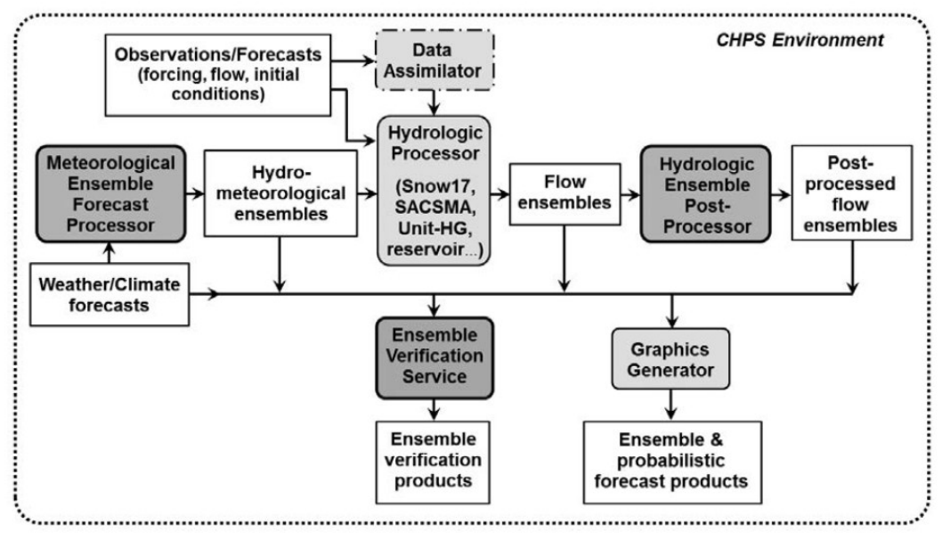
Figure 2.
Map of the study area.
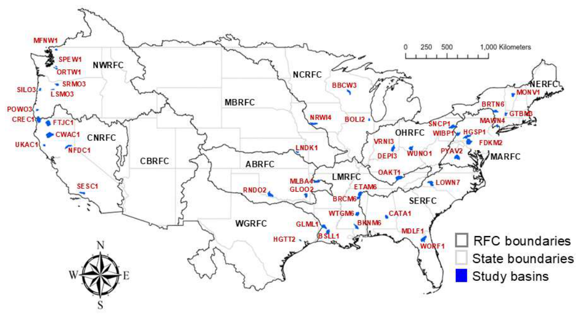
Figure 3.
Dataflow for the hindcast experiment (right) and AB_OPT (left).
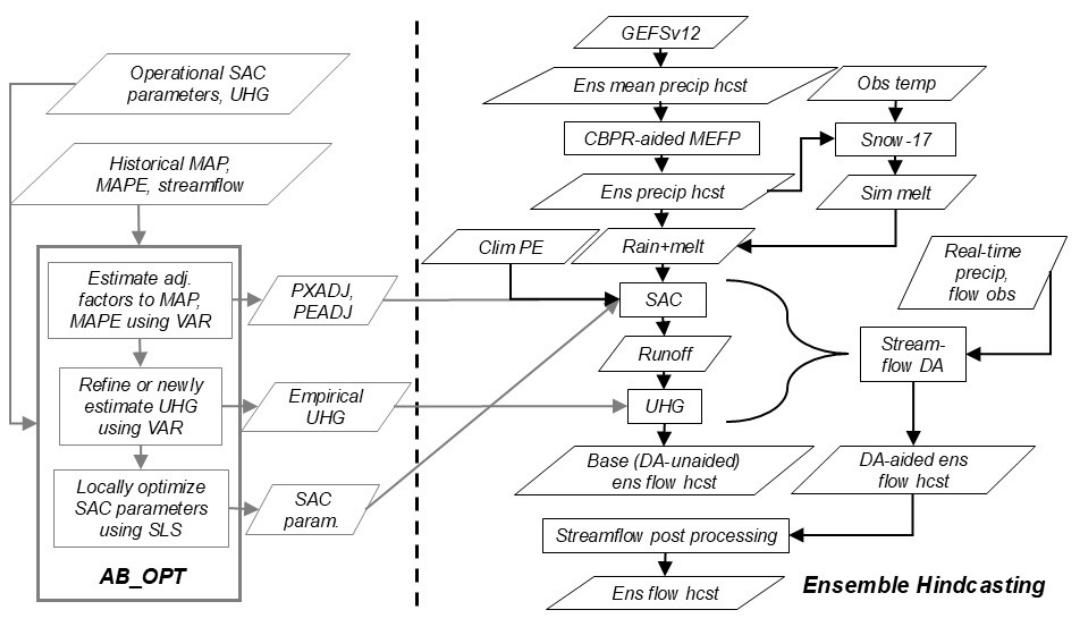
Figure 4.
Ensemble generation process for numerical integration of Eq. (4).
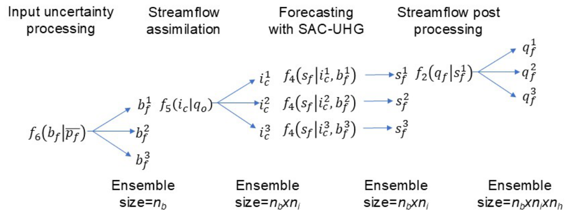
Figure 5.
CEs used in streamflow post processing with the CBPR-aided MEFP.
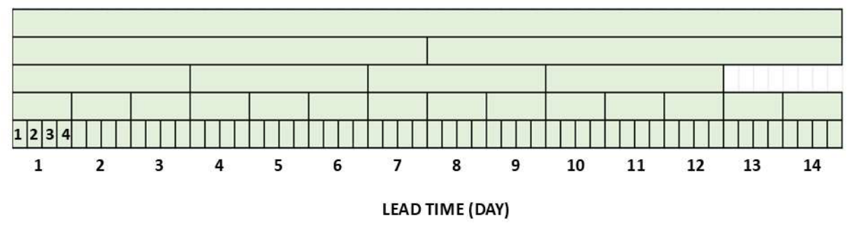
Figure 6.
CRPSS vs. lead time averaged over all locations of the base (i.e., DA-unaided) predictions (black), DA-aided predictions (red), post-processed DA-aided predictions (blue) and perfectly reliable (in the weak sense) post-processed DA-aided predictions (purple) under clairvoyant future input for a) all ranges of observed flow and observed flows exceeding the b) 90th, c) 95th and d) 99th percentiles. The reference is climatology. The number in parentheses in the plot title indicates the number of locations included.
Figure 6.
CRPSS vs. lead time averaged over all locations of the base (i.e., DA-unaided) predictions (black), DA-aided predictions (red), post-processed DA-aided predictions (blue) and perfectly reliable (in the weak sense) post-processed DA-aided predictions (purple) under clairvoyant future input for a) all ranges of observed flow and observed flows exceeding the b) 90th, c) 95th and d) 99th percentiles. The reference is climatology. The number in parentheses in the plot title indicates the number of locations included.
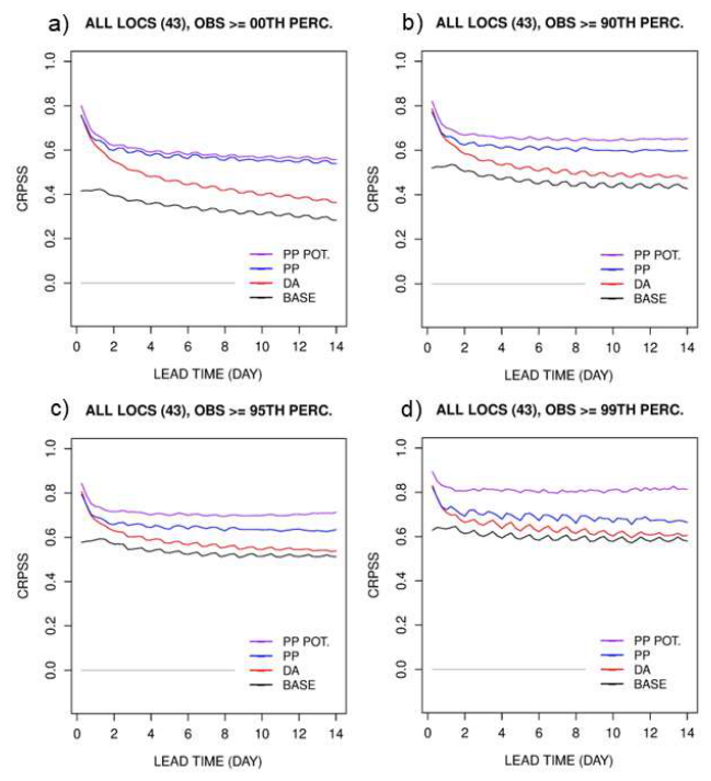
Figure 7.
Reliability diagrams of the post-processed DA-aided predictions of instantaneous flow under clairvoyant future input forcings for all 43 locations for lead times of 0.25 (top row), 4 (middle row) and 14 (bottom row) days and thresholds of 50th (leftmost column), 90th (middle-left column), 95th (middle-right column) and 99th (rightmost column) percentiles of observed flow.
Figure 7.
Reliability diagrams of the post-processed DA-aided predictions of instantaneous flow under clairvoyant future input forcings for all 43 locations for lead times of 0.25 (top row), 4 (middle row) and 14 (bottom row) days and thresholds of 50th (leftmost column), 90th (middle-left column), 95th (middle-right column) and 99th (rightmost column) percentiles of observed flow.
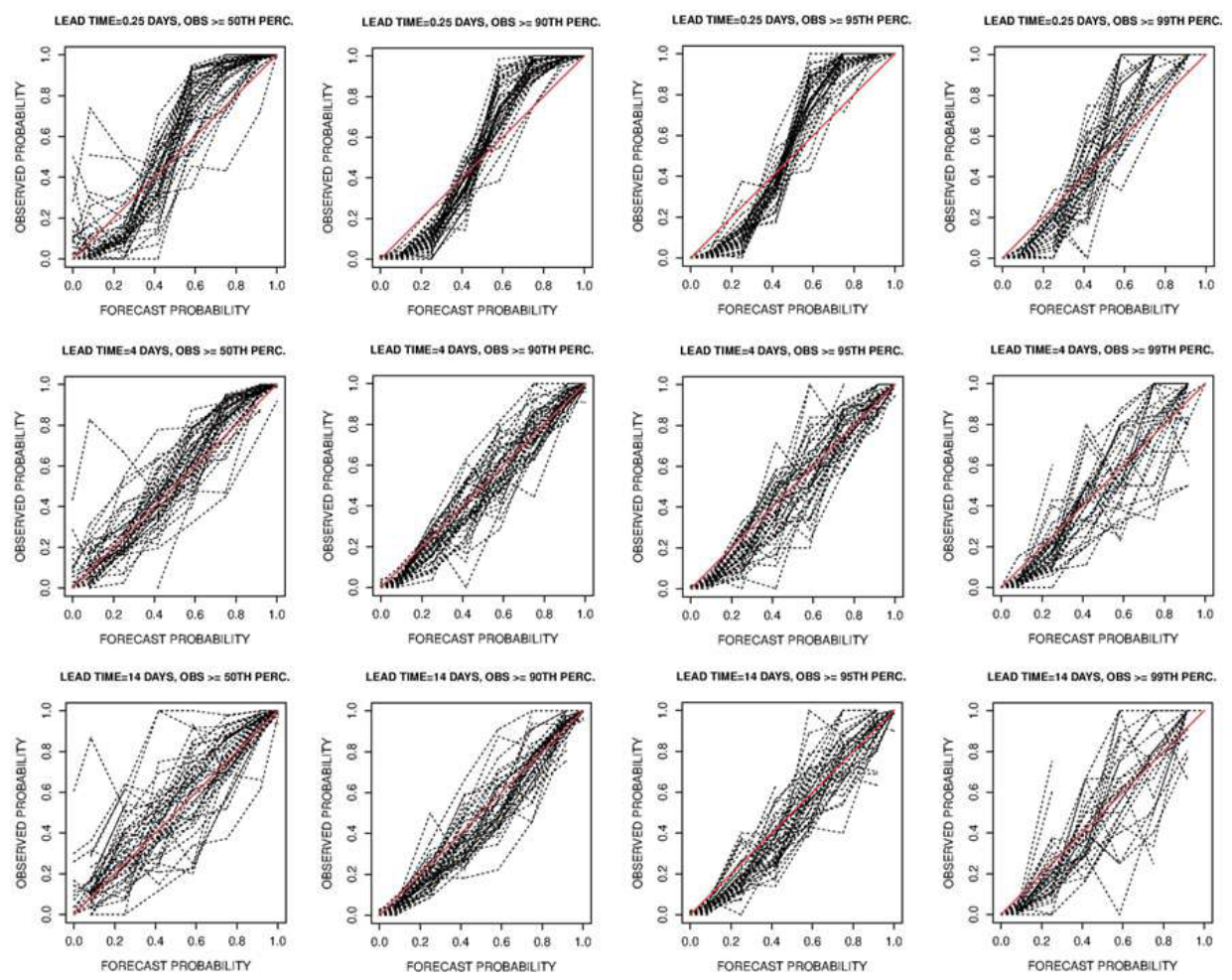
Figure 8.
AUC vs. lead time averaged over all available locations of the base (black), DA-aided (red) and post-processed DA-aided (blue) ensemble streamflow predictions under clairvoyant future input forcings. The conditioning events are the verifying observation exceeding the a) 50th, b) 90th, c) 95th and d) 99th percentiles. The number in parentheses in the plot title indicates the number of locations included.
Figure 8.
AUC vs. lead time averaged over all available locations of the base (black), DA-aided (red) and post-processed DA-aided (blue) ensemble streamflow predictions under clairvoyant future input forcings. The conditioning events are the verifying observation exceeding the a) 50th, b) 90th, c) 95th and d) 99th percentiles. The number in parentheses in the plot title indicates the number of locations included.
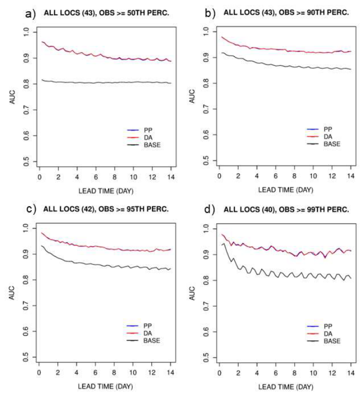
Figure 9.
CRPSS vs. lead time averaged over all locations of CLIMP (green), GEFS_CM (black), DA (red) and PP (blue) for a) all ranges of observed flow and the b) 90th, c) 95th and d) 99th percentiles of observed flow. The gray line, which is to be compared with the black line only, is based on the MEFP rather than the CBPR-aided MEFP.
Figure 9.
CRPSS vs. lead time averaged over all locations of CLIMP (green), GEFS_CM (black), DA (red) and PP (blue) for a) all ranges of observed flow and the b) 90th, c) 95th and d) 99th percentiles of observed flow. The gray line, which is to be compared with the black line only, is based on the MEFP rather than the CBPR-aided MEFP.
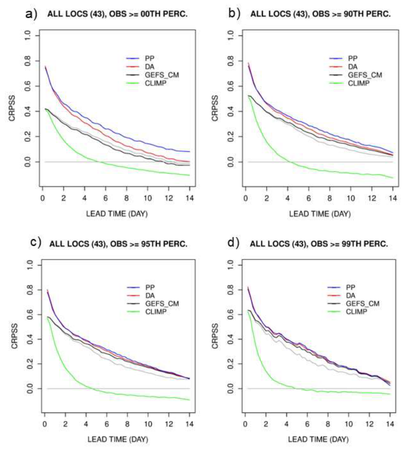
Figure 10.
Same as Figure 7 but under future input and hydrologic uncertainties.
Figure 10.
Same as Figure 7 but under future input and hydrologic uncertainties.
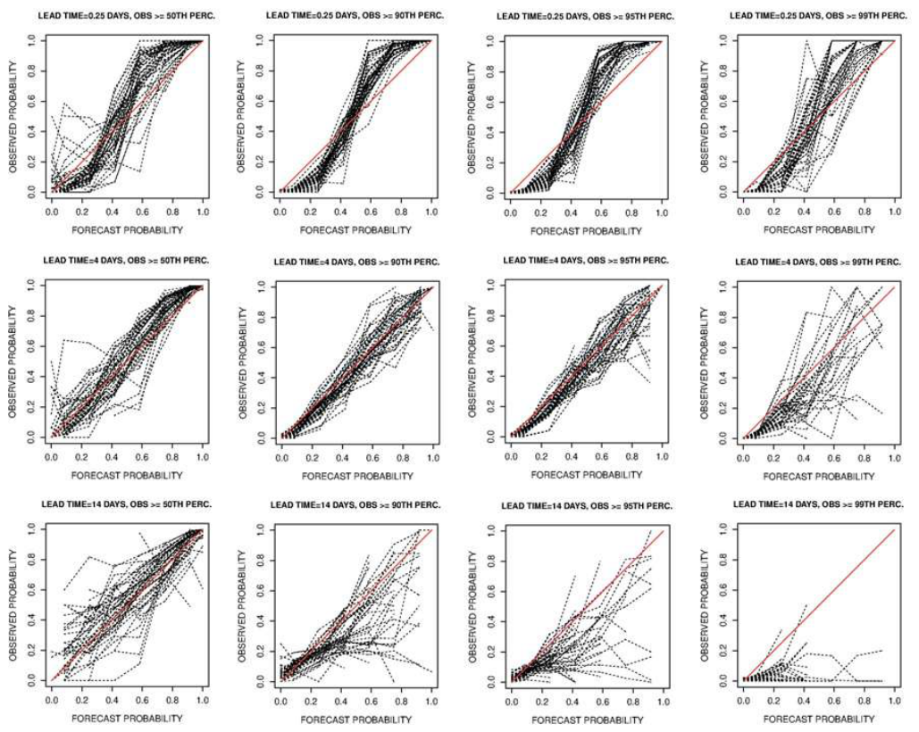
Figure 11.
Same as Figure 8 but under both future input and hydrologic uncertainties.
Figure 11.
Same as Figure 8 but under both future input and hydrologic uncertainties.
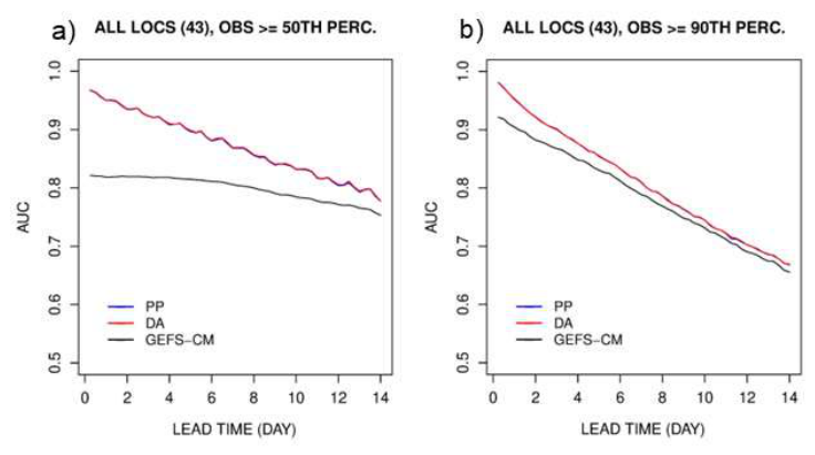
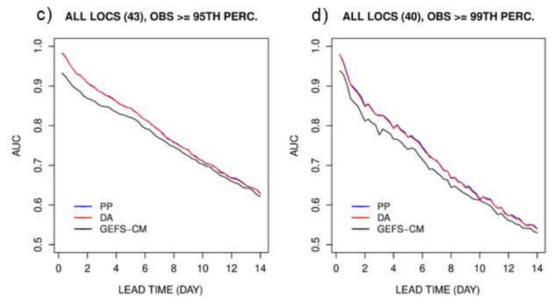
Figure 12.
CRPSS of CLIMP (green), GEFS_CM (black), DA (red) and PP (blue) averaged over all available locations in the a) CN- and b) OHRFC locations for all ranges of observed instantaneous flow. CRPSS of mean 6-hourly (cyan), daily (blue), 3-daily (green), weekly (red) and biweekly (black) PP for all available locations in the c) CN- and d) OHRFC locations for all ranges of observed flow. The parenthesized number in the plot title indicates the number of locations included.
Figure 12.
CRPSS of CLIMP (green), GEFS_CM (black), DA (red) and PP (blue) averaged over all available locations in the a) CN- and b) OHRFC locations for all ranges of observed instantaneous flow. CRPSS of mean 6-hourly (cyan), daily (blue), 3-daily (green), weekly (red) and biweekly (black) PP for all available locations in the c) CN- and d) OHRFC locations for all ranges of observed flow. The parenthesized number in the plot title indicates the number of locations included.
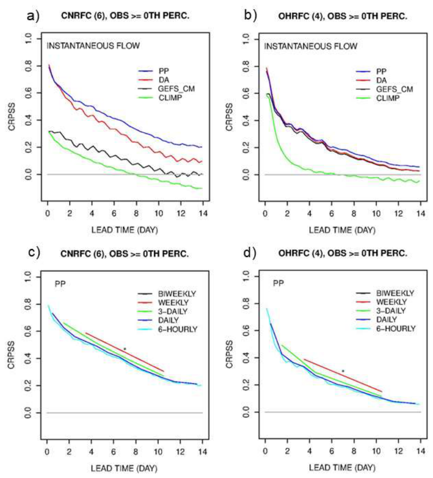
Figure 13.
Scatter (crosses) and QQ (red solid line) plots of ensemble mean predictions of 0-6 (leftmost column), 0-24 (middle-left column), 0-72 (middle-right column) and 0-168 (rightmost column) hr mean flow vs. verifying observed mean flow by GEFS_CM (top row), DA (middle row) and PP (bottom row). Each plot combines all 43 locations. BIAS is the ratio of the sum of all predictions to the sum of all verifying observations. CORR is the correlation coefficient.
Figure 13.
Scatter (crosses) and QQ (red solid line) plots of ensemble mean predictions of 0-6 (leftmost column), 0-24 (middle-left column), 0-72 (middle-right column) and 0-168 (rightmost column) hr mean flow vs. verifying observed mean flow by GEFS_CM (top row), DA (middle row) and PP (bottom row). Each plot combines all 43 locations. BIAS is the ratio of the sum of all predictions to the sum of all verifying observations. CORR is the correlation coefficient.
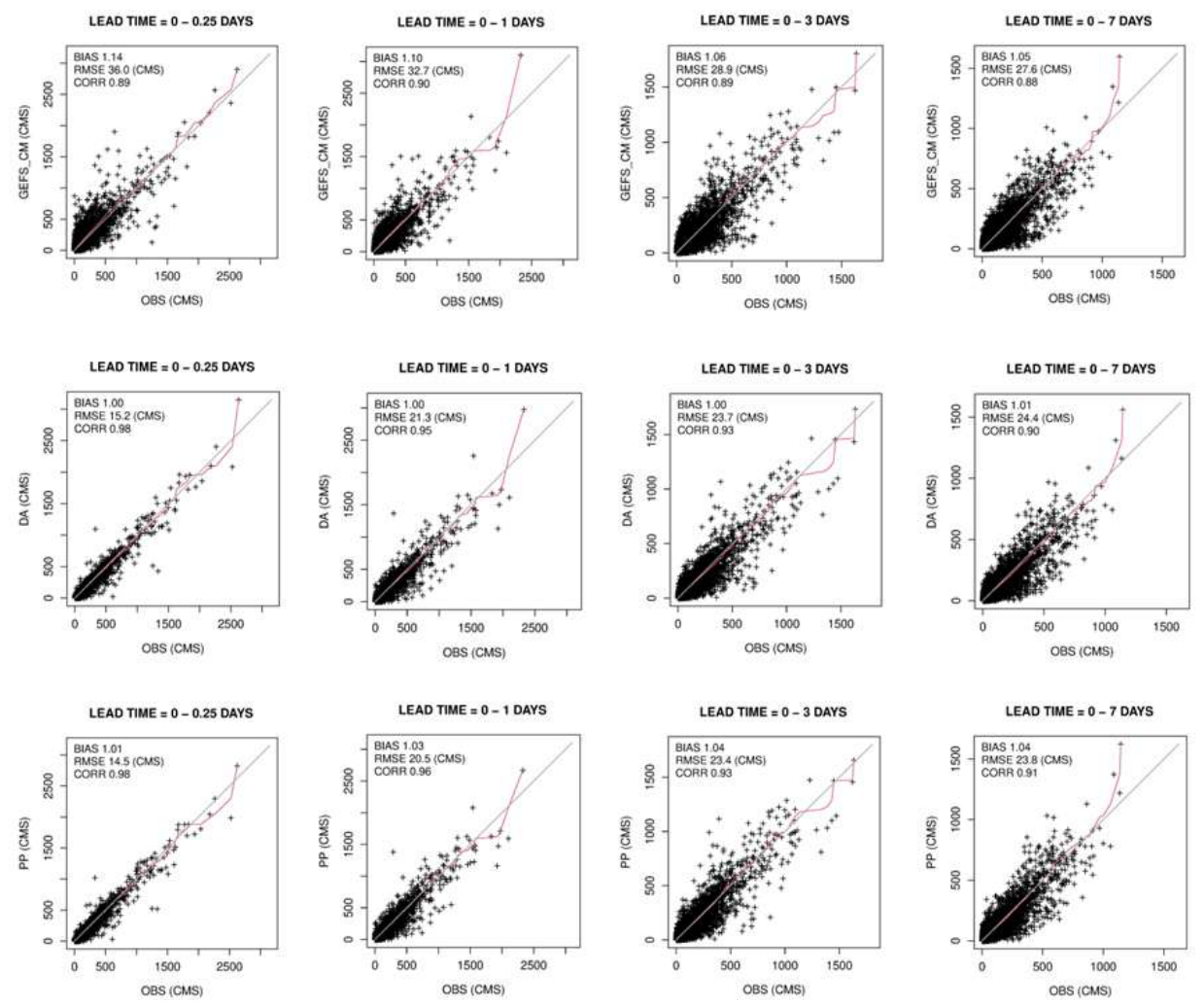

Table 1.
Streamflow forecasts assessed.
| Forecast name | Future precipitation used | ICs used | Stream-flow assimi-lation? | Stream-flow post process-ing? | Focus of assessment | Relevant components in Eq. (4) |
|---|---|---|---|---|---|---|
| CLIMP | Climato-logical ensemble precipitation forecast | Warm states | No | No | Quality of hydrologic modeling, strength of hydrologic memory | f4(sf| bf,ic) |
| GEFS_CM | Ensemble precipitation forecast from CBPR-aided MEFP forced by GEFS ensemble mean | Warm states | No | No | Impact of post-processed NWP precipitation forecast | |
| DA | Same as above | DA-aided warm states | Yes | No | Impact of reducing hydrologic IC uncertainty via streamflow assimilation | f5(ic| qo) |
| PP | Same as above | DA-aided warm states | Yes | Yes | Impact of reducing other hydrologic uncertainties via streamflow post processing |
|
Disclaimer/Publisher’s Note: The statements, opinions and data contained in all publications are solely those of the individual author(s) and contributor(s) and not of MDPI and/or the editor(s). MDPI and/or the editor(s) disclaim responsibility for any injury to people or property resulting from any ideas, methods, instructions or products referred to in the content. |
© 2026 by the authors. Licensee MDPI, Basel, Switzerland. This article is an open access article distributed under the terms and conditions of the Creative Commons Attribution (CC BY) license (http://creativecommons.org/licenses/by/4.0/).
Copyright: This open access article is published under a Creative Commons CC BY 4.0 license, which permit the free download, distribution, and reuse, provided that the author and preprint are cited in any reuse.