

Submitted:
01 October 2026
Posted:
05 October 2026
You are already at the latest version
Abstract
Manual annotation remains the source of ground truth for point cloud semantic classification, but its tools assume a contributor who can download billions of points and run desktop software. We present a browser-based framework that lets contributors classify remotely hosted datasets they neither own nor download. Points are labeled with a volumetric brush, and only the octree nodes the brush boundary crosses are fetched: regions fully inside are classified without being loaded, so the cost of a stroke follows its boundary rather than the points it encloses. Edits are held in a small ledger file, separate from the source data, that survives the discarding and reloading of points a streaming viewer performs and can be applied back to the source files at any time. Contributors receive disjoint regions as URLs and work asynchronously, returning ledgers that a project manager merges; classified subsets can also be exported as tiled LAS/LAZ. Class schemas are user-defined and travel with the edits. Where geometry alone is ambiguous, contributors label through pose-registered survey photographs. We demonstrate the framework on cultural heritage stonework, post-fire aerial LiDAR, and coral reef photogrammetry. It is open-source and deployed in production across OpenHeritage3D, the ALERTCalifornia Atlas Archive, and OpenOcean3D.
Keywords:
point cloud classification
; semantic segmentation
; crowdsourcing
; out-of-core editing
; point cloud annotation
; ground truth
; Potree
; LiDAR
; cultural heritage
; coral reef monitoring
1. Introduction
Affordable, high-precision three-dimensional sensing (terrestrial laser scanning (TLS), structure-from-motion photogrammetry, airborne light detection and ranging (LiDAR), and mobile mapping) has made the dense point cloud the primary record of both built and natural environments. Beyond the coordinates that fix each point in space, these sensors record per-point attributes: return intensity, RGB color transferred from co-registered imagery, and classification flags among other attributes written during initial processing. Those attributes are what make the data interpretable rather than merely geometric.
Semantic classification of a point cloud refers to the definition and assignment of certain classes or labels to each point based on a specified criterion [1]. Depending on the objective, it may be simply separating the ground from vegetation and man-made structures or it might include classifying individual architectural elements of an ancient building. Having a classified point cloud is crucial for various tasks including creating digital terrain models, volume calculation, feature extraction and 3D reconstruction, isolating or suppressing classes for measurement and visualization, and restricting change detection to comparable surfaces, as well as for generating training data for machine learning-based approaches, where data production now lags model development [2,3].
While desktop tools that support manual classification are available–CloudCompare, TerraScan, FARO Scene, Leica Cyclone, and Autodesk ReCap Pro being among them–a comparative evaluation of eight platforms found tool choice to be tightly constrained by user expertise, project scale, and scene complexity [4]. The binding constraint, however, is not which tool one picks but the locality all of them assume: the entire, possibly multi-terabyte dataset must be brought to the operator on their machine. While some specialists may possess the required hardware, many specialists and most volunteers do not. And if multiple contributors are involved, they must each possess a local copy of the original data.
Hierarchical octree streaming has moved point clouds off the specialist workstation and into the browser. Potree, a browser-based point cloud viewer [5,6], renders clouds of billions of points on commodity hardware with no data download and no software installation, and repositories including OpenTopography and OpenHeritage3D have built open-access archives on that infrastructure [7,8,9]. Access, however, has traveled further than editing. The browser-based annotation tools that do exist fall into two groups, neither of which reaches the data where it is published. The open-source group is small: 3D-Annotator offers brush, lasso, and polygon labeling of meshes and point clouds with project-level shared label sets [10], and the Semantic Segmentation Editor, developed for autonomous-driving research, labels PCD files against class sets fixed in a server-side configuration file [11]. Both load a full model into the client, and one release note of the latter marks the ability to label a one-million-point cloud as an improvement. The commercial group scales further, but on a service model: Flai classifies uploaded clouds with pretrained models over fixed category sets and bills per unit of processing [12], while Pointly pairs a browser viewer with automatic classification and an in-house labeling workforce [13]. Both require that the data be moved into the vendor’s environment. Across both groups, these systems are documented in repositories or vendor material rather than peer-reviewed literature, and to our knowledge, none of the open-source options can scale to very large datasets.
Both annotation labor and domain-matched training corpora have accumulated where capital is available: autonomous driving sustains paid annotation vendors, dedicated tooling, and full-time workforces, and the benchmarks that anchor the field (Semantic3D [14], S3DIS [15], ScanNet [16]) describe the urban and indoor scenes that comparably resourced programs have targeted. Heritage documentation, post-fire assessment, and reef ecology operate under a different profile: budgets are often small, the required expertise is scarce and does not transfer between projects, and datasets are one-off rather than continuously acquired. Labeled 3D data in these domains exists, with the ArCH dataset [17], the photogrammetric corpus of Pellis et al. [18], and NeMO-Net’s labeled reef scenes [19] among it, but coverage is thin against the range of typologies, sensors, and class schemas these fields encompass. Crowdsourced 3D annotation has shown that this labor can be distributed, with non-experts approaching expert accuracy on well-designed tasks such as urban tree extraction [20,21,22], but those deployments decompose the problem into pre-segmented object-level micro-tasks rather than free labeling against a full scene, and many distinctions these domains draw, between masonry types or coral species, do not reduce to questions an untrained worker can answer in seconds. What is missing is infrastructure that lets whoever holds the relevant knowledge label the data where it is already published: tooling that assumes no accounts, no backend, and no central database.
We present a collaborative classification framework implemented within the Potree viewer and deployed on the OpenHeritage3D, ALERTCalifornia Atlas Archive, and OpenOcean3D repositories. Contributors label points with a volumetric brush directly in the browser, against the full-resolution cloud, without downloading data or installing any software. A tiered octree traversal records each edit either as a whole-subtree assignment or as a set of per-point overrides, so that a stroke completely enclosing a region costs only a single ledger entry rather than millions, and network requests are confined to the boundary shell of the stroke. Edits persist in a portable ledger file that carries the classification schema and provenance metadata with it, decoupled from the original point cloud which may be hosted elsewhere. Work is distributed as URLs encoding disjoint sub-volumes, with no accounts and no server-side state, and returned ledgers combine through a deterministic merge before being applied to the source LAS/LAZ files or re-exported from the viewer. We demonstrate the framework across three domains: cultural heritage stonework, post-fire aerial LiDAR, and coral reef photogrammetry. Nothing in the system is specific to these; the class schema is user-defined rather than fixed in the implementation, and the only requirement on the input data is that it converts to LAS/LAZ for either Potree-format octree or COPC (Cloud Optimized Point Cloud) LAZ preprocessing, leaving sensor modality and application domain unconstrained. Nor is it specific to a kind of contributor: the same URL and ledger serve a lone specialist, a distributed research team, or a volunteer pool. Our emphasis on specialist annotation reflects where domain-matched labels are scarcest; what the framework removes is the hardware and software barrier, not the need for domain knowledge.
2. Literature Review
2.1. Interactive Editing of Out-of-Core Point Clouds
Interactive editing of large point clouds was addressed by Wand et al. [23], whose fully dynamic out-of-core octree supports real-time insertion, deletion, and modification of points, so that an edit is written into the hierarchy itself. Scheiblauer and Wimmer [24] separate the edit from the points, recording it as a Selection Octree defined over the space a selection encompasses rather than the individual points it contains, so that it survives level-of-detail refinement and can be written to disk and reloaded, though what it records is membership in a selection rather than an assigned class. They later showed that insertions and deletions must also update the interior nodes of such hierarchies, or visible artifacts remain [25,26]. In both cases the capability is embedded in a data structure designed for it (Scheiblauer and Wimmer’s Modifiable Nested Octree stores points in per-node grids precisely so that the model becomes editable), which places annotation behind a dedicated conversion of the source data into a locally held, editable copy.
Later systems likewise write edits into the data they display. Lin et al. [27] label point clouds of up to 50 million points in virtual reality using a combined CPU/GPU chunk structure with continuous level of detail, saving the result as a converted copy in their own format, and QGIS edits point attributes in locally stored COPC files by writing into the file itself [28]. Web-based systems for massive point clouds have instead concentrated on streaming and display, using per-point semantics to drive rendering and filtering [29]. Keeping edits apart from the source data has been explored for batch processing and versioning: PDAL’s EPT addons write batch-computed dimensions such as Classification to a hierarchy stored separately from an Entwine octree, so that write access to the source is not required [30], and Ogayar-Anguita et al. [31] version point clouds by storing only the changes between successive versions.
The framework presented here is built upon Potree [5,6], a popular browser-based point cloud viewer optimized for rendering large point clouds whose octree structure is based on Scheiblauer and Wimmer’s Modifiable Nested Octree. Potree on its own does not enable the user to modify point clouds and is intended largely for visualization. Our approach navigates around this restriction. Where our solution departs from the interactive systems above is that it treats the original point cloud as fully read-only and writes every edit into a separate edits ledger file (Section 3.5). Because an edit changes only a point’s class, never its position or its place in the hierarchy, the interior-node updates analyzed by Scheiblauer and Wimmer [25] do not arise. These shareable edits can be loaded on demand in the viewer and also be applied later to the original data (Section 3.6). This makes it so that any point cloud made viewable through Potree is editable with our framework without any additional preprocessing or modifications to the original data beyond what has already been performed to visualize it in Potree. The framework is compatible with both the native PotreeConverter 2.0 format [6] and the Cloud Optimized Point Cloud (COPC) LAZ format [32].
2.2. Crowdsourced Annotation of 3D Point Clouds
Crowdsourced geospatial data production has a long lineage in two dimensions, from OpenStreetMap and Volunteered Geographic Information onward, and that literature has consistently foregrounded quality and uncertainty as the central concerns in evaluating volunteer contributions [33]. Its extension to three-dimensional point clouds is more recent. Herfort et al. [20] established the pattern with a 3D micro-mapping framework in which non-experts extracted information from LiDAR point clouds of urban trees through web-based tasks solvable in under five seconds on average, reporting accuracies largely independent of the characteristics of either the input data or the individual worker, and identifying inter-volunteer agreement as a reliable intrinsic indicator of result quality. Walter et al. [21] subsequently examined how task decomposition, worker selection, and aggregation strategy govern the quality of crowd-derived labels, and Kölle et al. [22], Kölle et al. [34] combined crowd annotation with active learning for semantic segmentation of airborne LiDAR, finding that crowd-labeled training data trails a fully expert-labeled dataset by less than three percentage points in overall accuracy under appropriate sampling strategies. That annotation can be distributed beyond a single expert without a large loss in label quality is the premise on which the present framework builds.
These results are obtained under a common operational model. The annotation problem is decomposed into micro-tasks answerable in seconds (a pre-segmented tree in Herfort et al. [20], individual points selected by active learning in Kölle et al. [34]), those tasks are dispatched to volunteers or, in the later work, to paid workers through a commercial crowdsourcing marketplace, and quality is secured by collecting multiple independent judgements of the same item and aggregating them. Kölle et al. [35] carry this model to its conclusion in the CATEGORISE framework, which automates both worker employment and quality control so that a campaign can run without expert involvement, and the cost of sustaining paid redundant labeling is itself sufficiently pressing to have motivated gamification strategies for improving worker output [36]. The model presupposes a task server, a worker pool, and a dispatch pipeline. Within this same line of work, Kölle et al. [37] identify the construction of labeling interfaces usable by non-experts as an essential but frequently neglected problem, and note that three-dimensional data compounds it, since most workers have no prior experience with the data type.
The framework presented here departs from that model in both respects. Contributors label contiguous regions of the raw streamed geometry and draw class boundaries themselves, rather than answering isolated micro-tasks over objects or points selected for them, so no segmentation or sampling stage has to precede annotation. Assignment is carried entirely by a URL encoding a disjoint sub-volume, requiring no marketplace, no task server, and no contributor accounts, and returned contributions combine through a deterministic merge. What this model does not provide is consensus. Assignments are disjoint, so no two contributors label the same points, and the merge resolves conflicts by import order rather than by agreement, meaning that even deliberately overlapping assignments would yield a single surviving label rather than a comparison. The inter-annotator agreement that Herfort et al. [20] and Kölle et al. [22] rely on therefore cannot be computed within the framework, and any such analysis falls to the project manager outside it. Quality here rests on directing tiles to contributors with the relevant domain expertise and on review before merging, which is weaker than consensus and suited to the trusted-contributor setting these deployments assume. Section 6.5 sets out what a consensus-aware merge would require.
2.3. Automated Classification: State of the Art and Performance Gaps
The trajectory of point cloud segmentation research has been overwhelmingly model-centric: progress is measured in architectural innovations evaluated against a small set of fixed benchmarks, with comparatively little attention paid to assembling the labeled datasets those benchmarks depend on. Kölle et al. [2] argue for re-orienting the geospatial branch of the field toward the data-centric agenda of Ng [3]: a model is only as good as the data it learns from, and with high-frequency acquisition cycles, models generalize poorly enough that each new epoch may need its own training set. The critique applies with particular force to the domains addressed in this paper, whose class schemas bear little resemblance to those embedded in standard ALS or indoor-scene benchmarks.
Deep learning has advanced point cloud semantic segmentation from PointNet [38] through hierarchical architectures [39], graph convolutional networks [40], and transformer-based models [41], and leading models perform strongly on well-characterized benchmarks such as Semantic3D [14] and S3DIS [15]. Even on benchmarks, however, fine-grained classes lag: on the UAV LiDAR benchmark Hessigheim 3D, baseline classifiers reach 75–77% mean F1, with the lowest scores on soil/gravel and urban furniture, classes the benchmark added to its predecessor’s catalog [42].
These limitations become acute in the domains addressed by this paper. In heritage, Grilli and Remondino [43] show that a random forest trained on one set of buildings generalizes to others of similar architectural character but performs worst on a stylistically different one, and conclude that distinct architectural categories should be treated with separately trained models. Heritage segmentation is further complicated by over-segmentation, by divergent results between laser-scanned and photogrammetric data of the same scene, by a shortage of dedicated benchmarks, and by class schemas that require domain expertise to annotate correctly [44]; the dedicated datasets that now exist [17,18] are each bound to the typologies and acquisition conditions of the buildings they document.
Ecological and post-fire monitoring sharpen the problem in different ways. For coral reef survey, standard ALS and indoor-scene benchmarks carry nothing corresponding to benthic categories such as live coral, dead coral, rubble, and encrusting algae, so a classifier must be trained against a schema no general-purpose corpus supplies. For post-fire assessment the schema often remains nominal, but automated classification of it can itself be unreliable: in the deployment described in Section 4.2, outcrops and flat canopy were misread as structure and tree–building interfaces in dense parcels resolved ambiguously [45]. These errors are sparse and spatially scattered, which is what makes them expensive to locate and correct.
These limitations motivate a data-centric, human-in-the-loop approach in which automated pipelines provide approximate classification at scale while contributors correct their errors, apply schemas the pipelines never carried, and supply the interpretive judgment that ambiguous surfaces require. The tool presented here is therefore positioned not as a classifier but as annotation infrastructure: its deterministic merge assembles contributor work into provenance-tracked labels that can in turn train automated classifiers, a cycle between human annotation and machine learning [22].
2.4. Crowdsourcing Annotations Within Coral Reef Ecology
Marine and reef ecology has been an unusually productive testbed for annotation infrastructure. Imagery volumes far beyond expert capacity, taxonomic expertise concentrated in relatively few people, and an ecosystem the public will readily volunteer time for have together driven the field to build assisted labeling, consensus aggregation, and open annotated corpora ahead of comparable environmental domains, and much of what it has produced generalizes past marine science. The resulting landscape is bifurcated. On one side is a mature ecosystem of 2D platforms designed primarily to accelerate expert workflows and collaborative analysis. At the center of this is CoralNet, a cloud platform for point-based annotations and automated cover estimation that operationalizes the tradeoff between speed and accuracy for trained annotators [46]. TagLab takes a region-based rather than point-based approach, pairing CNN-assisted segmentation of orthoimages with manual refinement of the resulting polygons, and a user study of coral community segmentation reported an increase in annotation speed of approximately 90% for non-expert annotators with labeling accuracy preserved [47]. ReefCloud applies a similar AI-assisted workflow, reported to reduce manual analysis time and cost while maintaining high agreement with expert validation [48]. Squidle+ provides web-based management and annotation of marine imagery, allowing large datasets to be shared across teams [49]. Others include MERMAID, which standardizes field data collection and integrates with AI classifiers [50], and CeruleanAI, which lowers the barrier to large-scale monitoring through automated photomosaic stitching and built-in analysis [51]. What these share is a focus on accelerating expert 2D analysis rather than on open public contribution.
The second branch draws on public citizen science to manage the overwhelming volume of marine imagery. The Great Reef Census analysis platform exemplifies this by having virtual volunteers assign class labels to AI-generated polygons, relying on repeated consensus averaging to balance crowdsourced effort with high accuracy [52]. Generalized platforms also play an important role; Zooniverse hosts dedicated projects like Click-a-Coral, which asks volunteers to classify benthic life in deep-sea video and imagery to iteratively train AI models [53]. Another approach is the FathomNet and FathomVerse ecosystem [54,55], which pairs a globally accessible database of expert-annotated images with an interactive mobile game that actively crowdsources bounding-box annotations from the public to train future computer vision models. The common thread is harnessing global citizen science through intuitive, engaging interfaces to generate the labeled datasets required to train and refine marine computer vision models, and neither the task decomposition nor the aggregation strategies these platforms rely on are specific to reefs.
By contrast, systems designed for public crowdsourcing of 3D coral reef data (e.g., point clouds, meshes) remain rare, despite the growing adoption of Structure-from-Motion workflows [56]. The principal example is NeMO-Net, a purpose-built, gamified platform that allows players to paint semantic labels directly onto 2D and 3D reef scenes [19]. Because 3D annotation is inherently complex, NeMO-Net relies on substantial platform engineering, using tutorials, active-learning loops, and weighted consensus aggregation to manage data quality and ecological label ambiguity. While engaging with 3D models helps volunteers improve recall, the NeMO-Net literature highlights the challenges of visual ambiguity and the technical burden of sustaining a standalone 3D crowdsourcing environment.
That a field this far along in 2D annotation infrastructure has produced one such system is itself the measure of the gap: to our knowledge, no accessible platform allows an independent researcher to put their own 3D reef survey in front of contributors and collect annotations on it. That gap has two halves. The framework presented here addresses the annotation half, for data already published through a streaming repository, by removing the need to build and host a standalone platform; it does not replace the training and consensus machinery NeMO-Net uses to manage untrained volunteers, and is suited instead to the trusted-contributor setting described in Section 2.2. The other half, a place where completed annotations can be deposited against a dataset and seen by others, belongs at the repository layer rather than in the viewer (Section 6.5). Until both halves exist, collaborative mapping and scalable analysis of 3D reef photogrammetry will remain limited.
3. Methods
3.1. Overview
We present a point cloud classification interface implemented as an extension to Potree, a WebGL point cloud viewer. The system enables contributors to assign semantic labels to points across large datasets entirely in the browser, without downloading source data or installing point cloud software. The central technical challenge is that Potree’s octree architecture was designed purely for visualization: only a small working subset of the point cloud is held in memory at any time, and nodes are routinely evicted and reloaded from disk as the camera moves. Any classification change written directly to a geometry buffer is therefore ephemeral. Our solution is a tiered traversal that marks fully enclosed subtrees with a single ledger entry rather than loading their points, confining the cost of a stroke to its boundary shell, with edits persisted in that ledger independent of node residency. The remainder of this section describes that pathway and the components built around it: two routes to obtain a classified LAS/LAZ file, user-definable classification schemas, the collaborative classification workflow, and the oriented-photograph mode used where geometry alone is ambiguous. Figure 1 summarizes the complete system.
3.2. System Architecture and Design Decisions
The framework runs entirely in a web browser against static Potree-format or COPC LAZ files served over HTTPS. No files are written or modified server-side, and no backend services are required beyond a standard static file host. We decided against the alternative of the contributor writing edits back to server-side copies of the source data due to three factors:
1. Storage: Point cloud datasets routinely surpass hundreds or thousands of gigabytes. Maintaining a per-contributor copy of such a file is infeasible at any realistic scale: even a handful of concurrent contributors would exhaust the host’s storage, and the copies would be largely redundant, since classification typically touches only a small fraction of points.
2. Access Control: Writing to shared source files requires user accounts, role-based permissions, and conflict resolution for concurrent edits. That infrastructure is expensive to build and difficult to maintain, and it is ill-suited to repositories like OpenHeritage3D, where datasets are shared under Creative Commons licenses and the contributor population is open and distributed.
3. Portability: A framework that depends on custom backend services can be deployed only by institutions willing to run them. Restricting the architecture to static file serving means any existing Potree deployment can integrate the classification interface by including a single JavaScript file, with no server modifications. Contributors, in turn, need nothing beyond a browser: annotation demands no more of their hardware or connection than viewing the dataset does, and far less than the download-and-install workflows it replaces.
Therefore, all the classification work done by the contributor lives in the client memory as a ledger (Section 3.5) of edits. This ledger of edits can then be exported as a relatively small file which then can be imported back into the viewer to enable persistence across page reloading.
3.3. Volumetric Brush
Selection in point-based editors has long been posed volumetrically rather than in screen space: Weyrich et al. [57] introduced a brush that follows the sampled surface using nearby depth values, Bürger et al. [58] used spherical GPU brushes for sub-voxel volume editing, and Scheiblauer and Wimmer [24] carried the metaphor out-of-core, defining the selection on the space the brush encloses rather than on the points, so that it survives level-of-detail changes. Annotation tools today offer either screen-space lasso selection, which also captures occluded background points, or a movable sphere [10].
In our implementation, the brush is a world-space sphere (Figure 2). After opening the Classification Brush interface (Toolbar Tools Classification), the contributor selects a class and paints by holding Ctrl/Cmd and dragging across the point cloud. It is drawn as a translucent wireframe tinted with the color of the active class, so the brush previews the label it will write; camera rotation is suspended while Ctrl/Cmd is held so a stroke cannot drag the view.
The radius is specified in world units rather than screen pixels, so a stroke covers the same physical extent regardless of viewing distance. It is initialized from the scene scale when the panel opens, and set on a logarithmic slider spanning 1 mm to 100 m, typed in meters, stepped by 20% with the Q and E keys, or changed mid-stroke by holding Ctrl/Cmd and moving the scrollwheel. The brush is toggled from the panel or with the Z key.
Opening the panel switches the viewer from RGBA rendering to a composite mode blending RGB color with a classification overlay, so assigned classes are visible without obscuring the point colors; the blend is adjustable from the panel and cycled with the W key. Contributors can hide individual classes to focus on unlabeled regions, and a dropdown targets one point cloud or all visible ones, useful where an aerial scan and a photogrammetric model of the same site overlap.
Each stroke casts a ray through the cursor position; Potree’s native pick function returns the closest intersected point on the target cloud, and the active classification is assigned to all points within the brush radius of that intersection. Node loading, traversal, and buffer assignment are described in Section 3.4.
3.4. Tiered Octree Traversal and On-demand Point Classification
Potree uses an out-of-core rendering algorithm: the full point cloud lives on disk or remote storage, and only a working subset is held in browser memory at any time. The data is organized as a hierarchical octree [5] in which each node stores a subsample of the points within its bounding region, with finer subdivisions at deeper levels. Potree loads only those nodes that intersect the current frustum, and within those, it loads finer levels selectively based on distance to the camera.
This suits fast visualization but not editing, since a brush stroke can cover points the client has not loaded, whether they lie outside the visible region or below the currently requested level of detail. Naively, this would restrict classification to the points a contributor can currently see, with finer points either silently skipped or only made editable by increasing the global point budget or moving the camera closer. For small datasets this may be acceptable, but our target use case makes both workarounds untenable and asking contributors to navigate the camera into every region they want to edit defeats the purpose of a brush (Figure 3).
An obvious approach would be to traverse the octree from the root, load every node whose bounding box intersects the sphere, and for each point in those nodes perform a sphere-distance check, apply the new class if successful, and record the edit in the ledger (Section 3.5). However, this approach does not scale since increasing the brush radius results in the number of intersected nodes growing approximately quadratically for surface data. Because loading is asynchronous and bounded by network and disk throughput, and because every point in every loaded node must be tested individually, even moderate brush sizes can require loading thousands of nodes per stroke on dense datasets from disk, producing multi-second latencies that hinder interactive use.
The key insight motivating our solution is that during painting, many nodes’ bounding boxes are entirely contained within the brush sphere, which implies that all of that node’s descendants and points are also contained. For such nodes, neither the node data nor that of any descendant needs to be loaded or inspected: the entire subtree can be marked with the target classification as a single ledger entry. We exploit this observation through a tiered traversal algorithm that evaluates three conditions at each node, proceeding from cheapest to most expensive (Algorithm 1).
| Algorithm 1 Tiered traversal for on-demand point classification. |
|
When the contributor performs a stroke, the function is invoked with the octree root. In the first tier, each node’s axis-aligned bounding box (AABB) is tested against the brush sphere; nodes that fail the intersection test are pruned along with their entire subtrees. Given the size of the brush sphere relative to the full point cloud, most of the octree is rejected at this stage. In the second tier, for nodes whose bounding box is entirely contained within the sphere, the algorithm records a single implicit ledger entry marking the entire subtree with the target classification, without loading or inspecting any point data. Any descendant ledger entries that are now superseded are cleaned up by prefix-matching on octree node names (Potree’s naming convention guarantees that parent names are string prefixes of their descendants). If the node’s data happens to already be resident in memory, the classification buffer is filled directly; otherwise, the fill is deferred to the reconciliation hook described in Section 3.5. The function then returns without recursing further into the subtree.
The second tier is also subject to a visibility gate that prevents it from silently overwriting points whose classification is currently hidden in the contributor’s panel. The system maintains a 256-entry lookup table mapping each classification value to its visibility state, populated once per stroke. When all classes are visible and there are no volume clipping boxes intersecting the node, the bulk assignment proceeds. When points are hidden, the algorithm falls through to the third tier, which performs per-point inspection and respects visibility on a point-by-point basis. This ensures that a contributor painting over a region with hidden points does not accidentally reclassify points they cannot see, which could silently overwrite work by a previous annotator whose classes are toggled off or are clipped by a volume selection.
The third tier handles nodes at the boundary of the brush sphere, where only some points are inside. These nodes are force-loaded asynchronously if not already resident, and every point is tested against the sphere. Before testing, any existing ledger state for the node (inherited baseline fill plus per-point overrides) is applied to the geometry buffer so that the distance test operates on the correct current classification. Points are skipped if their current class is hidden, already matches the target class, or if they are clipped by a volume selection. Classified points are recorded as per-point overrides in the ledger (Section 3.5), and the classification buffer is flagged for GPU upload so the renderer reflects the change on the next frame. The function then recurses into each child, with siblings traversed concurrently so that multiple subtrees requiring network fetches can load in parallel. The effective baseline classification, the nearest implicit-mark entry in the ancestor chain, is threaded as a parameter through the recursion rather than re-derived at each node.
In this manner, we restrict the slowest part of the algorithm, the asynchronous node loading, to only execute for partially intersecting nodes rather than naively loading every intersecting node. Therefore, instead of growing with the enclosed surface area, quadratically in brush radius, as for the naive traversal, this tiered approach grows as the length of the surface boundary grows (that is dependent on circumference instead of area). An additional optimization reduces the cost of per-point distance testing. Within each node, the brush center is transformed into the node’s local coordinate frame via a single matrix inversion, rather than transforming every point into world space. Since each node may contain thousands of points but only one center needs transformation, this reduces the per-node linear algebra cost from matrix multiplications to one.
After each stroke completes, a promotion pass examines nodes that received per-point overrides during the stroke. If every point in a node has been classified to the same value and the overrides unanimously cover all points, the per-point map is promoted to a single implicit-mark entry, compacting the ledger and reducing both memory usage and future synchronization cost.
An earlier iteration of this algorithm restricted traversal to nodes intersected by the picking ray, on the assumption that ray-intersected nodes would form a small superset of the relevant ones. In practice, this approach missed nodes that intersected the brush sphere without intersecting the ray itself (a common occurrence when the brush radius is large relative to the cursor’s distance to the surface), and the savings in nodes visited were modest, since AABB pruning already eliminates most of the tree. We therefore adopted the full-traversal approach described above.
Because nodes (mainly partially intersecting nodes) may need to be fetched from disk or over the network, the latency of a brush stroke depends on how much of the affected region is already resident in memory. Strokes near the camera, where nodes are typically already loaded at high detail, complete almost instantly; strokes that require loading deep or distant subtrees take longer, bounded by network and disk throughput. The tiered approach significantly mitigates this: interior nodes that are fully contained produce no network requests at all, so only the thin shell of boundary nodes at the sphere surface requires loading. For instance, if one were to paint an object in its entirety in one stroke with minimal partial intersection, no asynchronous loading would occur and the operation would be instantaneous.
To prevent overlapping strokes from producing inconsistent classifications during slow loads, the brush blocks new strokes until the current one completes, with a visible status indicator showing that loading and classification are in progress. The most recent pending stroke is retained so that the contributor’s last cursor position is always honored.
3.5. Edit Persistence: Tiered Ledger and Node Reconciliation
The tiered traversal described in Section 3.4 produces classification changes that are written directly to geometry buffers in GPU-accessible memory. However, as mentioned before, these changes are ephemeral: Potree routinely evicts nodes that fall outside the visible region or move too far from the camera, and when such nodes are later reloaded from disk or remote storage, they arrive with their original, unmodified classification values. To ensure that classification work survives node eviction and reloading, we maintain an edit ledger: an in-memory data structure that records every classification decision made during the session, independent of which nodes are currently resident.
The ledger is structured as a nested map keyed first by point cloud name, then by octree node name. The first type, an implicit-mark entry, records that an entire subtree has been assigned a single classification. This entry stores only the classification value and carries no per-point data; it is produced by the second tier of the traversal when a node’s bounding box is fully contained within the brush sphere. The second type, a per-point override map, records individual point classifications keyed by buffer index within the node. This is produced by the third tier for boundary nodes where only some points fall inside the brush sphere. The third type, a hybrid entry, combines an implicit-mark baseline with an explicit per-point override map. This arises when a subtree has been bulk-classified but a subsequent stroke at its boundary modifies only some of its points to a different class.
Baseline inheritance exploits Potree’s octree naming convention, in which parent node names are string prefixes of their descendants (e.g., “r0” is a prefix of “r03”). When applying the ledger to a node, the system walks up the name hierarchy by successively truncating the last character until it finds an implicit-mark entry or reaches the root. The classification from the nearest such ancestor becomes the effective baseline for all descendants that lack their own entry. This means that a single implicit-mark entry at a high level of the tree implicitly defines the classification of potentially thousands of descendant nodes without storing any per-descendant data. Per-point overrides, when present, are then applied on top of this baseline.
To synchronize the ledger with the rendered scene, we register a callback on Potree’s node-loading pipeline that fires the instant a geometry buffer is created for any node. When the callback is triggered, the system queries the ledger for the node’s entry and its inherited baseline, fills the classification buffer with the baseline value if one exists, and overlays any per-point overrides. Because the reconciliation is event-driven rather than poll-based, freshly loaded nodes are brought into agreement with the ledger before they are first rendered, eliminating the visual flicker that earlier poll-based approaches produced when a previously-edited node was reloaded and momentarily displayed its original, unmodified classification.
Since the ledger lives only in browser memory, edits are lost on page reload. The system allows the contributor to save their editing session by exporting the ledger as a file and later resume by importing it. Two export formats are provided, differing in the coordinate space they record. The Potree-Only export serializes the ledger structure verbatim, including implicit-mark directives and per-point override indices, for re-import into the viewer; because it addresses points by their index within an octree node, it requires no node loading regardless of dataset size. Each node’s override indices are run-length encoded as a binary stream and the file is gzipped, while the metadata and schema header remains plain text so that a returned ledger stays identifiable without opening the viewer. The world-space export instead resolves implicit regions to axis-aligned bounding boxes and explicit overrides to world coordinates, written as a gzipped CSV for downstream patching of LAS (LASer point cloud format) files (Section 3.6.1); it loads only those nodes carrying per-point overrides, never entire implicitly-marked subtrees, so its cost follows the number of boundary edits rather than the total classified volume. Even on multi-million-point datasets the Potree ledger stays small enough to share by email or version control (Section 4.3). These classification edit ledgers can be shared with other users who may import them and continue to build upon another’s classification work (detailed in Section 3.8).
3.6. Applying Classification Changes to the Point Cloud on Disk
Contributors often need the modified point cloud as a LAS/LAZ file on disk for downstream processing or machine learning applications. We provide two pipelines: a lightweight script that patches the original files using the exported ledger, and an in-browser export of the modified region. The patch pipeline suits refinement workflows where edits affect a small fraction of a large dataset; the export pipeline is preferred when fresh classifications cover large regions or when the original files are not available.
3.6.1. Patching the Original Point Cloud via the Ledger
When edits are sparse relative to the full dataset, the original LAS/LAZ files can be patched directly from the world-space export (Section 3.5) using a Python script. The script accepts either a single LAS/LAZ file or a directory of tiles, and either a single World-Space export file or a directory of them; in the latter case all are merged before processing, allowing a project manager to apply multiple contributors’ edits in a single pass.
The script applies edits in two phases that mirror the ledger’s tiered structure. In the first phase, each AABB region exported from an implicit ledger entry is matched against the LAS file: every point whose coordinates fall within the bounding box is assigned the region’s classification. Because a merged export may contain thousands of regions, the file’s points are sorted once along one axis so that each region binary-searches to the slice of points it can possibly contain, rather than scanning every coordinate array in full. Regions are applied in ascending order of the octree depth they were exported from, sorted globally across all input files, so that a deeper region always supersedes the ancestor containing it; this reproduces the baseline inheritance of Section 3.5, under which the nearest implicit-mark ancestor determines a point’s class. In the second phase, per-point overrides exported from explicit and hybrid ledger entries are matched to their nearest LAS points by world-space position using a KD-tree nearest-neighbor lookup, with a configurable distance threshold (default 0.01 m) to accommodate the coordinate quantization of the export and floating-point drift introduced by Potree’s transformations between the source files and the in-browser octree. Overrides are applied after AABBs and take precedence, preserving the ledger semantics in which per-point corrections at sphere boundaries supersede bulk region assignments.
For each input file, a bounding-box pre-filter rejects both AABBs and override candidates that fall entirely outside the file’s spatial extent, so tiles that no edit touches are read but not searched. Original geometry and all non-classification attributes are preserved; only classification values are modified.
3.6.2. Direct Export from the Web Interface
The entire updated point cloud, or a part of it, can also be downloaded directly from the web interface (Toolbar Tools Download Selection). After opening the menu, the contributor must make one or more volume-box selections, and choose the desired level of detail; the point cloud is then served to the contributor as one or more LAS files.
We utilize the native Potree getPointsInBox3() function which returns all points in a specified volume by recursing through the nodes until a given depth. A major limitation of implementing this naively is that all returned points must be held in memory simultaneously, then serialized to LAS format and offered as a single download. This drastically constrains the maximum selection size to what the browser’s JavaScript heap can hold. For dense surveys this can be exceeded by even modest selections, causing the tab to fail before serialization completes.
Our solution divides the selected volume into a grid and serializes each tile as a separate LAS file while skipping empty tiles. This keeps the in-memory point buffer bounded regardless of the total selection size and the download remains steady. To choose an appropriate grid resolution, we account for the varying point densities of different datasets (a single tile size would either fragment a sparse dataset unnecessarily or overflow memory on a dense one) by dynamically selecting the grid size as follows. Let V be the selection volume, the estimated point density at the requested level of detail (LOD), and B the target point budget per tile, for which the default is , which we found keeps peak memory below approximately 2 GB on the test machines used during development. Potree’s octree generator targets approximately 5,000 points per node. Therefore the total tile count is
Given the selection’s horizontal footprint and with aspect ratio , tiles are distributed across X and Y to preserve that aspect:
This produces tiles whose horizontal proportions roughly match the selection’s footprint, so very elongated selections aren’t tiled into long thin strips, with on the assumption that the selection is significantly broader than it is tall, which holds for aerial LiDAR, most heritage surveys, and reef datasets. For vertically-extensive datasets such as TLS scans of multi-story interiors or coral reef columns, manual override of the grid dimensions is supported via the API.
For the density estimate , since Potree’s octree stores points at progressively finer spacing with depth, density at depth d is approximated from the root spacing as
Potree halves the point spacing at each octree level, so the volumetric density at depth d is the cube of the inverse of the spacing at that level. This estimate is computed per visible point cloud and summed across the selection.
The export pipeline also supports classification-based filtering: any class toggled off through the brush panel’s classification visibility controls is excluded from the exported LAS files. The filter is applied during the same index-collection pass that tests points against the selection box, so hidden points are rejected with a single array lookup before any spatial test or attribute copy. The cost of filtering is negligible relative to the cost of exporting. This is useful in several recurring scenarios: extracting an irregularly-bounded feature that cannot be cleanly enclosed by a box selection (a single building, a stand of vegetation, the ground surface beneath it); pre-segmenting a dataset for downstream analysis by exporting each class as an independent file; or stripping noise classes (e.g., LAS class 7) to produce a clean point cloud ready for direct use. In every case the result is a smaller, more targeted export that reduces the post-processing burden typically borne by tools such as CloudCompare, PDAL, or bespoke scripts.
We also provide a level-of-detail control slider in the UI that caps octree traversal depth, allowing the contributor to trade resolution for download size and time. The slider’s range is read from the loaded dataset’s metadata so it reflects the actual depth of the source octree. Additionally, an expected average point density is displayed.
Before each tile is queried, ledger edits intersecting that tile’s bounding box are reapplied to the relevant octree nodes, force-loading them if necessary (Section 3.4). This guarantees the exported file reflects all classification changes regardless of which nodes happen to be resident in memory at the time of export.
Finally, each tile is written as a separate LAS file via Potree’s LAS exporter. When the browser supports the File System Access API, all tiles and a JSON manifest are written into a single user-selected directory; otherwise the browser falls back to staggered individual downloads. The manifest records the source digital object identifier (DOI), citation, generation timestamp, selection bounds, tile grid, and per-tile point counts to support provenance and downstream reassembly. The manifest serves as a self-contained provenance record, allowing exported tiles to be traced back to their source dataset and the specific download parameters used, consistent with the broader archival principles of the OpenHeritage3D infrastructure.
3.7. Configurable Classification Schemas
The American Society for Photogrammetry and Remote Sensing (ASPRS) defines a set of classification codes for the LAS format [60]. For LAS 1.4 and 1.5, codes from 0–18 are used for features such as vegetation, water, and ground, and 19–63 are reserved. That leaves 64–255 to be user-definable. Since we present our system as serving researchers and contributors across various disciplines, we provide the ability to create custom classes, in the user-defined range (64–255) as suited to a particular use case and ensure compatibility with downstream LAS processing tools that expect ASPRS-compliant files.
For example, reef ecologists classifying coral photogrammetric models may define species-level classes such as Acropora, Porites, and Orbicella, or morphological categories such as bleaching, healthy, and new growth, distinctions that bear no relationship to the ASPRS standard schema. Similarly, architectural surveys may require classes for specific masonry types or structural elements, and post-fire assessments for burn severity gradations not present in any standard schema.
To define a custom class, the contributor may open the “edit” menu (Toolbar Tools Classification Edit) and input a new classification name, color, and number. After this, the new classification will be added as another brush color next to the default classifications.
The classification schema is embedded in the ledger file header and restored automatically when the file is imported, so a contributor working on coral taxonomy doesn’t have to reconfigure the class list each session. The schema embedded in the ledger file must be consistent across contributors working on the same dataset; project managers are responsible for distributing a canonical schema file before annotation begins (Section 3.8) and they may do so by either directly providing the file to each contributor or placing it alongside the point cloud on the server so that it loads automatically.
The panel also provides a convenient visibility toggle for each classification, allowing the contributor to hide points of a particular class and prevent them from being targeted by the brush.
3.8. Work Distribution and Aggregation
Although manual classification of dense point clouds is in principle parallelizable across multiple annotators, and while commercial software does support parallel work through shared project databases (e.g. Leica Cyclone SERVER, TerraScan’s block-based projects), that model presumes licensed installations within a single administrative domain and a full local copy of the data, which does not extend to contributors outside that domain, whether specialists at other institutions or a wider public, annotating a publicly hosted archive. Datasets in specialist communities frequently require diverse subject matter expertise (masonry types, coral species, certain landscape features) that no single contributor possesses. This section describes the workflow by which a project manager subdivides a dataset into spatial assignments, distributes them to contributors with the relevant expertise, and aggregates returned classifications into a single ground-truth dataset (Figure 4).
To initiate, the project manager opens the “Work Distribution” menu (Toolbar Tools Classification Work Distribution), creates a master clipping volume around the region to be classified, and chooses a grid resolution (1–8 per side via the menu slider, producing up to 64 tiles). The system then subdivides the master volume into an grid of sub-volumes. Similar to our LAS export tiling pipeline (Section 3.6.2), we preserve the Z extent and split along X/Y as the selection is generally significantly broader than it is tall. Each sub-volume also inherits the master’s rotation. After the creation of the grid, each sub-volume is assigned a unique A1-style grid reference such as A1, A2, or B3.
Subsequently, each sub-volume is serialized to a compact string (encoding position, rotation, scale, and clip state) and is embedded as a query parameter in a viewer URL. The project manager obtains a list of URLs, each with a different sub-volume encoded, each of which is assigned to a different contributor. When a contributor opens their assigned URL, they see only the points inside their assigned sub-volume. The purpose of this is threefold: it focuses the contributor only on their region without requiring them to navigate manually; it creates a soft boundary which prevents contributors from accidentally classifying points in another contributor’s tile since there are no overlapping points; and clipping also reduces rendering cost, since Potree skips rendering points that lie entirely outside the clip volume. To minimize coordination overhead, the URL is the entire assignment artifact: there is no server-side coordination, no central database, no contributor accounts, no central state. A manager can distribute assignments via email, Slack, a spreadsheet, or any other channel.
Every contributor then uses the brush tool (Section 3.3) to classify points only in their assigned volume, exports the ledger file, and returns it to the manager via any file-sharing channel. The ledger file itself is generally quite small, as it contains only records of the modified points (Section 3.5). The project manager first imports each ledger edits file individually to check for outliers and spatial overlap (rare, given tile-based assignment, but a contributor may accidentally classify points outside their tile), and then imports all edit files together. When multiple files contain entries for the same octree node, the import performs a structural merge: implicit and explicit entries for the same node combine into hybrid entries, and per-point overrides from the later import take precedence on conflict, so that overlapping contributions compose correctly without requiring manual reconciliation.
As discussed in Section 3.6, we provide two pipelines for the acquisition of the modified point cloud on disk. The project manager may choose to patch the original point cloud’s LAS file (Section 3.6.1) by selecting the folder containing the LAS tiles (or a single LAS file) and the folder containing the ledger files (or a single ledger file), which results in the creation of the edited LAS files. Alternatively, the project manager may import all edit ledger files in Potree at once, review the entire dataset, and then use the direct export pipeline (Section 3.6.2).
In an effort to provide versioning, provenance, and quality control functionality, the ledger file itself contains several key metadata fields including: the contributor name (optional, manually entered by the contributor), generation timestamp, point cloud name(s), tile index, number of modified points, project DOI, and project citation.
The classification schema can be stored alongside the point cloud on the server and loaded automatically when a contributor opens an assigned URL. This avoids the need for the project manager to distribute a separate schema file and guarantees that all contributors annotate against the same class definitions. Contributors retain the ability to define additional custom classes locally (Section 3.7), but the canonical schema for the dataset is fixed by the project owner and travels with the dataset itself.
The framework reduces collaborative annotation to two lightweight artifacts: a URL that carries the assignment, and a small edits file that carries the result.
3.9. Photograph-Referenced Annotation
Where the point cloud alone is insufficient to make out finer details of the model (e.g. in the case of coral classification: distinguishing bleached colonies from pale substrate), consulting the original survey photographs is the only available disambiguator. While Potree offers support for displaying oriented images, the feature does not integrate well with our volumetric brush painting system by default.
Therefore, we extended the base oriented image functionality as follows: focusing a photograph locks the camera to that image’s pose, so image and cloud remain registered for as long as the image is open, with an opacity slider cross-fading between them; the cloud behind is rendered in pure classification color so that class boundaries read against the photographic detail rather than competing with it. The brush continues to operate on the geometry while an image is focused: strokes pass through the photograph and classify the underlying points, with the image serving only as reference. Holding Shift while brushing names the photograph nearest the cursor and Shift-clicking opens it, so a contributor working an unclear region reaches the best available photographic view of that region without leaving the stroke. On exit the previous blend setting is restored. Section 4.3 exercises this on reef photogrammetry, where colony identification frequently depends on it.
3.10. Use of Artificial Intelligence
The AI tool Claude.ai, using the Claude Opus 5 large language model [61], was used to revise portions of the text and in the later stages of the literature review to search for highly specific relevant sources related to the paper’s subject matter. It was also employed to suggest grammatical corrections to original text, to improve clarity and flow. The authors of this paper have reviewed and approved the final manuscript, and take full responsibility for its content, including the content which has been generated or modified by AI tools.
4. Case Studies
4.1. Cultural Heritage
An essential part of architectural analysis of built cultural heritage is semantically classifying architectural elements, as downstream evaluation often concerns individual element types rather than the structure as a whole. Carnevale [62], for example, fits ellipsoidal models to column shafts extracted from point clouds of the Pantheon and other Roman, Byzantine, and Renaissance monuments to determine shaft radii, entasis profiles, and inter-columnar spacing, analyses that require isolated column geometry at controlled point densities, not the surrounding walls, floors, or roof.
In a conventional workflow, such an analysis begins by downloading the full multi-gigabyte dataset, loading it into desktop software such as CloudCompare, manually segmenting the columns of interest, subsampling to the desired density, and exporting the result, a process that may take hours for a single building and requires both significant disk space and specialist software proficiency. In the framework presented here, the same researcher can instead classify the columns directly in the browser, toggle off all other classes to isolate them, and export only the column points at a user-selected level of detail through the download tool (Section 3.6.2). The exported file contains only the geometry relevant to the analysis, and the classification is recorded in the ledger for reuse by other contributors.
The dataset in this study is a terrestrial laser scanning point cloud consisting of about 6M points from the Bern Digital Pantheon project, acquired between 2005 and 2008 using a Cyrax 2500 scanner and distributed through the OpenHeritage3D repository [63]. The Pantheon’s portico offers a well-suited test environment: its Corinthian columns, entablature, pediment, walls, floor, and doorway present clearly delineated architectural elements whose geometric regularity facilitates visual assessment of classification quality, while the building’s canonical status in architectural history makes the demonstration immediately legible to a broad audience.
A contributor classified the portico facade into eight semantic classes: column, wall, floor, door, arch, pediment, entablature, and roof. Six of these (column, wall, floor, door, arch, and roof) correspond to standard classes in the ArCH benchmark [17], while pediment and entablature were added through the classification editor as user-defined classes (Section 3.7), demonstrating the system’s ability to extend the default LAS schema to accommodate finer architectural distinctions than ArCH’s roof and moulding categories permit (Figure 5a). Classification was performed using the brush tool in the composite rendering mode, which blends the original RGB point colors with a semi-transparent classification overlay (Figure 5b). This mode preserves surface detail, including the Agrippa dedicatory inscription on the frieze, stone texture, and capital ornamentation, while providing continuous visual confirmation of the active class assignment, eliminating the need to toggle between raw and classified views during annotation.
The resulting ledger illustrates the opposite regime from the reef plot (Section 4.3). It assigns a class to 6,068,400 points (99.9% of the cloud, including 140,702 explicitly set to Unclassified; the remaining 7,898 retain their original LAS class) through 1,000 entries: 340 implicit, 134 hybrid, and 526 explicit. Here 77.7% of the assigned points are stored as per-point overrides. The octree has only 1,001 nodes, holding roughly 6,000 points each, so its nodes are coarse relative to the architectural elements, and a stroke tracing a column or moulding rarely encloses a node’s bounding box whole. Baselines carry at most 37% of any class (roof), while entablature, pediment, and arch, the classes requiring the finest boundaries, are stored almost entirely per point. The exported ledger is 91.2 kB, or 0.12 bits per point. The same labels stored at one byte per point would occupy 6.08 MB uncompressed and 140 kB gzip-compressed in octree order, so even with most points stored individually the ledger is about a third smaller, though at this scale the difference is immaterial.
The selective extraction this workflow demonstrates extends naturally to any element-level analysis of historical architecture: proportional studies of arches and vaults, planarity assessments of wall surfaces, or geometric documentation of moulding profiles.
By coupling semantic classification with targeted export, the framework transforms the point cloud from a monolithic dataset requiring wholesale download into a queryable spatial archive from which researchers can retrieve precisely the elements they need, and the classified outputs can serve as labeled training data for the domain-specific segmentation models whose absence the ArCH benchmark highlights.
4.2. ALERTCalifornia Post-Fire LiDAR
The classification framework was deployed as a refinement step within a volumetric damage characterization of the January 2025 Palisades and Eaton fires [45]. That study used multi-temporal aerial LiDAR differencing across 37,500 acres of wildland-urban interface, with carbon emission estimates stratified by surface type (building, vegetation, and unclassified) derived from the pre-fire epoch’s automated LAStools classification. The automated pipeline produced systematic but spatially sparse errors: rock outcrops and flat tree canopies misclassified as buildings, and ambiguous tree-building interfaces in dense urban parcels. The Palisades collection alone comprises 5.93 billion points, with the Eaton collection adding a further 1.17 billion [64,65].
This sparsity makes conventional desktop correction impractical at scale: the errors are scattered across hundreds of tiles spanning both fire perimeters, so an operator would first need to identify which tiles require attention, retrieve them, correct them individually, and re-export. In the framework presented here, contributors instead navigated directly to visible errors in the browser, corrected them with the brush tool within assigned sub-volumes (Section 3.8), and exported only the sparse edits as a ledger file. The corrections were applied back to the original LAS tiles through the patching script (Section 3.6.1), leaving all unmodified points untouched. After refinement, the companion study’s per-structure envelope cross-check and cross-validation against an independent atmospheric inversion [66] confirmed that the corrected classifications produced volumetric and emission estimates within expected bounds.
The brush tool was also used as a measurement instrument to characterize residual mixed-pixel edge artifacts along building perimeters: false height differences introduced when LiDAR pulses straddle rooftop-ground boundaries at different scan geometries between epochs (Figure 6). A statistical sample of 75 destroyed buildings was inspected using the brush, finding 13,817 erroneous points out of 525,688 building-classified points, bounding the artifact contribution at approximately ±5% of building-class volume [45]. The artifacts themselves were retained in the production data and handled by the differencing threshold rather than removed.
4.3. Coral Reef Health Assessment
To exercise the work distribution and merge workflow of Section 3.8 from end to end, a multi-contributor classification effort was performed on a coral reef dataset from Palmyra Atoll [67]: a dense photogrammetric model of reef plot FR38, acquired in 2019 as part of a long-term monitoring effort tracking coral growth at fixed sites. The model spans approximately and comprises 455,673,460 points at a ground sample distance of about 1 mm. The project manager first defined a custom schema of six reef-relevant classes (healthy coral, dead coral, bleached coral, substrate, algae, and other) through the classification editor (Section 3.7), assigning them codes 64–69 in the user-definable range of the LAS specification. The manager then created a master Work Distribution volume over the plot and selected a grid, subdividing it into nine disjoint sub-volumes, hereafter referred to as tiles, labeled A1 through C3 (Figure 7a). Nine URLs, one per tile, were generated and distributed to the contributors.
Each contributor followed the same procedure within their assigned tile, requiring approximately one hour per tile. The tile was first classified in its entirety as substrate, a bulk assignment that the ledger captures almost entirely as implicit whole-node entries (Section 3.5). The remaining classes (healthy, dead, and bleached coral, and algae) were then painted over this base with the volumetric brush in the composite rendering mode, with the RGB/classification blend adjusted as needed: at intermediate blend values the photogrammetric color remains visible through the class tint, so colony boundaries can be traced without toggling between raw and classified views (Figure 8).
A crucial part of the contributor’s workflow here was utilizing the original survey images as reference when the point cloud was not sufficiently detailed to distinguish certain features (Figure 9). The feature is described in detail in Section 3.9.
The resulting labels should be read as illustrative rather than authoritative; the contributors possess widely varying degrees of identification expertise. Class assignments were made by visual inspection, without taxonomic field guides or field validation, thus individual assignments may be inaccurate. However, the case study does strongly demonstrate the mechanics and throughput of the distributed workflow on reef morphology, which was the only intention. The precise statistics on the distribution of each of the categories are not intended to be authoritative and representative of the dataset as they are merely intended to illustrate the implications of the system’s data structure organization and the effect discordant classes have on file-size.
Each contributor exported their work as a ledger file whose metadata block records the contributor name, generation timestamp, tile reference, source dataset and DOI. The project manager imported all nine files, which merged deterministically into the complete classification shown in Figure 7b, reviewed the merged result for coverage and boundary consistency, and exported the fully classified point cloud through the download tool (Toolbar Tools Download Selection; Section 3.6.2).
The merged ledger also shows how the tiered representation behaves on a fully classified dataset. This is the worst case for an edit ledger, since nearly every point carries an assigned class, and the best case for the alternative of storing a class value per point. The ledger holds 61,892 node entries: 23,645 implicit, 318 hybrid, and 37,929 explicit. The 23,963 implicit and hybrid baselines assign the class of 375,159,831 points (82.3%) without any per-point data. The remaining 80,410,167 points are recorded as individual overrides, so the ledger stores 17.7% of the records a per-point encoding would require. The split between tiers follows the structure of the annotation (Table 1). Substrate, 63% of the cloud, is carried almost entirely by 25 entries in the top four levels of the octree, with only 1,425 substrate points stored individually. Healthy coral colony interiors are carried by 21,104 baselines, 93% of them at depths 7 and 8. Fragmented classes shift toward explicit storage, reaching 90% for algae, which is the degradation toward per-point classification as brush size approaches node size noted in Section 6.1. Explicit entries lie where class boundaries pass: 99.2% of explicit and hybrid nodes contain more than one class.
The exported ledger occupies 3.16 MB (0.055 bits per point), against 455.7 MB at one byte per point and 73.2 MB (1.29 bits per point) for any encoding that treats labels as independent. The fair baseline is lower: because Potree stores points grouped by octree node and labels are spatially coherent, the class array gzip-compresses in octree order to 6.04 MB. The ledger is about half that size, but its main advantage is not compactness: it is the structure the viewer edits, merges, and resolves against nodes it has not loaded.
5. Evaluation of the Tiered Traversal
We evaluate how the cost of a stroke scales with brush radius under the tiered traversal of Section 3.4, against a naive traversal that loads and inspects every node whose bounding box intersects the brush sphere. A stroke here is a single application of Algorithm 1. The primary measure is the number of nodes a stroke must inspect: nodes that must be resident in memory and whose points are tested individually. These bound the network requests a stroke can issue, and on remotely hosted data a request costs orders of magnitude more than the per-point distance tests it enables (Section 6.1), which are therefore reported only as a secondary measure. Latency is not reported, since it depends on which nodes happen to be resident and on network conditions, whereas node counts depend only on the octree and the stroke.
For surface data, the naive count should grow with the surface area the sphere encloses and the inspected count of our implementation with the length of the curve along which the sphere cuts the surface, so on logarithmic axes their slopes should differ by approximately one (Section 6.1); the absolute slopes depend on surface roughness and are not themselves the prediction. Because octree nodes are cubic, a node of edge length w can lie entirely inside a sphere of radius r only if , so no saving is expected until the brush exceeds the size of the octree nodes at the stroke location. We therefore report radius both in meters and as , where w is the edge length of the deepest node containing the brush center.
Strokes were applied programmatically to the FR38 reef plot (Section 4.3) at a single brush center, where the deepest node lies at depth 8 with m, at four radii ranging from below to a sphere enclosing the entire plot. Each stroke began from an empty ledger, with all classes visible, no clipping volume active, and a target class absent from the data. Naive counts were computed from the dataset’s full octree hierarchy.
Table 2 and Figure 10 trace the transition from per-point to implicit classification as the brush grows. At no node was enclosed, and the stroke inspected the same 12 nodes a naive traversal would, nine of them the path from the root to the leaf containing the brush center. At the tiered traversal inspected 1,114 of the 6,355 nodes the sphere intersects, and implicit marks assigned 85.5% of the classified points; at it inspected 3,003 of 75,970, and the implicit share reached 96.7%. Between these two radii the naive count grows as and the inspected count as , a difference of 1.16 against the predicted value of about one; with one brush center and two radii, these exponents are indicative only. At m the sphere encloses the octree root, and a single implicit mark classifies all 455,673,460 points without inspecting any node, where a naive traversal would inspect all 147,905.
6. Discussion
6.1. The Rendering Octree as an Edit Index
Pruning a spatial index against a query volume is not itself a contribution; any competent volumetric brush would arrive at the first tier of Algorithm 1. What differs in the out-of-core web setting is what pruning purchases: a fully in-memory application saves a per-point distance test costing nanoseconds when it rejects a subtree, while here it saves a network round trip, five to six orders of magnitude more expensive, so the traversal is better understood as an I/O scheduling policy than a query optimization. The second tier follows from this and has no direct counterpart in a conventional range query: because classification is a uniform overwrite rather than a per-point computation, a fully enclosed subtree is completely described by a node identifier and a target class, so recording it as a single ledger entry makes both edit cost and ledger size scale with the boundary length of the brush rather than its enclosed surface area, letting a contributor classify points they have never loaded. That surface-boundary scaling is not itself a new result: Hunter and Steiglitz [68] established that the cost of region operations on a quadtree is proportional to the perimeter of the region rather than to its area, and the generalization to octrees and to higher dimensions is standard [69]. What differs here is the quantity being conserved, which is not arithmetic but network round trips against an octree the client neither owns nor can reorganize. The scaling is also asymptotic in the ratio of brush radius to leaf-node extent, and degrades toward per-point classification as the brush shrinks toward node size—precisely the regime of fine boundary correction, the most time-expensive part of annotation.
6.2. Latency at the Boundary Shell
Nodes straddling the brush surface cannot be resolved without inspection, so a stroke blocks on fetching them, and latency in this regime is governed by the trip time to storage rather than by client-side computation the framework can further optimize (event-driven loading, raised in-flight concurrency, and batched GPU flushes already extract what is available on the client). Server-side spatial query would collapse the boundary shell into one request but reintroduces the backend processing the static-file architecture was chosen to avoid (Section 3.2); resolving strokes against whichever level of detail happens to be resident would trade away boundary fidelity precisely where it matters most, since, for instance, Runyan et al. [70] found that both inter-labeler disagreement and neural-network error concentrate at coral colony boundaries. The more promising direction, not yet implemented, is coalescing the boundary shell into fewer HTTP range requests by exploiting the spatial adjacency of boundary nodes within PotreeConverter 2.0’s binary node layout [6], trading some over-fetching for fewer round trips.
6.3. Limitations of the Current Implementation
The most consequential limitation concerns quality control. The ledger’s reported total-edits count is exact for explicit per-point overrides but only approximate for implicit subtree entries, since an unloaded subtree’s true point count is not known until its hierarchy has fully resolved; more importantly, sub-volume assignments are disjoint by construction (Section 3.8), so no two contributors ever label the same points, leaving no redundant observations from which to compute the inter-annotator agreement that Herfort et al. [20], Runyan et al. [70], and NeMO-Net [19] each use as their primary quality signal: the framework provides provenance, not validation. This also produces a seam problem at sub-volume boundaries, where adjacent contributors may label a continuous surface inconsistently; the merge workflow surfaces the worst of these for manual review but does not automate conflict detection, and over-granular or ambiguous class schemas compound the risk by introducing annotation noise that propagates into downstream training data.
The framework is also scoped to semantic classification alone. Every point receives a single integer class code written to the LAS classification field, and the ledger carries no notion of object identity, so two adjacent coral colonies assigned the same class are indistinguishable in the output. Instance and panoptic segmentation would require a per-point object identifier of far greater range than the byte-valued ASPRS field affords, stored as a separate attribute, together with an interface for delimiting individual objects rather than painting regions; both lie outside the problem addressed here. A related consequence of the architecture is that the framework has no undo or redo functionality, a consequence of not storing previous and original per-point classifications (Section 3.5), which is architecturally incompatible with implicit marks over unloaded subtrees; a bounded stroke-level undo built from an inverse ledger diff and snapshots of touched resident buffers is designed but not implemented. Browser constraints add further limits: JavaScript’s single-threaded execution caps how far per-point testing can exploit multi-core hardware, browser memory limits bound how much of the octree can be resident at once, and mobile and tablet devices generally lack the headroom for interactive work on dense point clouds, restricting practical use to desktop and laptop hardware.
6.4. Dependencies and Portability
The classification layer makes no graphics API calls; it interacts with Potree and three.js only through the node-load completion hook, geometry attribute buffers, the octree node-naming convention baseline inheritance depends on, and the volumetric query underlying export. The browser-wide migration from WebGL to WebGPU, and the corresponding rebuild of Potree on WebGPU named Potree-Next, are consequently transparent to this layer as long as equivalent abstractions are exposed. A rebuild that reorganizes the node loading pipeline or node-naming scheme would require re-engineering the traversal and reconciliation layers regardless of which API sits underneath.
6.5. Scalability and Future Directions
The nearest-term priority is the validation infrastructure the current design omits: redundant or calibration-tile assignment and automated inter-annotator agreement over the resulting overlap would convert the framework’s provenance guarantees into quality guarantees. Server-side pre-segmentation, offering contributors initial label suggestions to refine rather than generate in the active-learning style of Kölle et al. [22], is the most promising route to higher throughput, well matched to concentrating human effort at the boundaries where automated methods are least reliable; integration with emerging 3D foundation models would let the framework both produce training data and consume model outputs in the same loop. Because every oriented photograph carries a known pose and calibration, a classified cloud can also be rendered from that pose into a per-image label mask, propagating one three-dimensional annotation to every photograph observing the same surface and yielding 2D labels from 3D effort.
Consensus aggregation is the most consequential absent capability. The ledger already records per-point overrides and a contributor field, so the information a consensus merge would need is present in the artifacts; what is missing is a merge mode that retains divergent entries for the same point rather than resolving them by import order, and a reporting layer that surfaces disagreement rates per tile and per class. Combined with deliberately overlapping assignments, which the URL scheme already permits, this would recover the inter-annotator agreement measures that the current disjoint model forgoes.
Additional features such as filtering points by RGB, elevation, intensity or other attributes rather than by geometry alone would speed up the workflow for power users. Selecting, for instance, only points whose color falls above a green threshold within the brush volume in order to label algal cover in a single pass, which is well matched to the fact that contributors already read color and intensity when deciding a class.
Finally, the artifact the framework produces is already suited to an infrastructure it does not provide. A ledger is small, self-describing, and carries the dataset DOI, source, contributor, and timestamp of the work it records, so a repository that accepted ledgers keyed to a published dataset would let contributions accumulate, be browsed, and be reused by anyone working on that dataset, closing the half of the gap identified in Section 2.4 that this work leaves open. Such a service necessarily reintroduces server-side state, which is why it belongs at the repository layer rather than in the viewer. Integration with repository infrastructures such as OpenHeritage3D, ALERTCalifornia Atlas Archive and OpenOcean3D [8,9] offers a natural pathway to reach contributors beyond the teams that produced a dataset, from domain experts at other institutions to students and volunteers, though opening contribution this widely requires sustained investment in onboarding materials, calibration datasets, and governance balancing openness against rigor. The framework presented here is a first step toward the labeled point cloud commons the data-centric paradigm requires [2,3].
7. Conclusions
This paper presented a browser-based framework that brings manual point cloud classification to datasets where they are already published, letting contributors label large remotely hosted datasets that they neither own nor download. A volumetric brush drives a tiered octree traversal that assigns fully enclosed subtrees with a single ledger entry and fetches only the nodes the brush boundary crosses, so that both the network cost of a stroke and the size of its record scale with the boundary of the classified region rather than with the points it encloses. That traversal adapts established out-of-core selection to an octree the contributor does not control; the framework’s principal contribution is the ledger in which edits are held, a portable file decoupled from the source data that survives the eviction and reload of streaming, carries its user-defined class schema and provenance, and can be applied to the source LAS/LAZ files at any time. Collaboration requires no accounts, backend, or central database: it reduces to a URL encoding a disjoint sub-volume and the ledger a contributor returns, which a project manager merges deterministically before patching the source files or exporting classified subsets as tiled LAS/LAZ. Where geometry alone is ambiguous, contributors can label through pose-registered survey photographs. Three deployments—architectural stonework, post-fire aerial LiDAR, and reef photogrammetry—show the same interface carrying selective element extraction, sparse correction of an automated classifier across 7.1 billion points, and a multi-contributor annotation of a reef plot consisting of 455M points whose complete classification the ledger encodes in 61,892 entries. The system is specific neither to these domains nor to specialist contributors; its only requirement is that input data convert to LAS/LAZ for Potree-format or COPC streaming. The principal limitation is that the framework offers provenance without validation: because assignments are disjoint by construction, no redundancy exists from which to compute inter-annotator agreement, and closing that gap is the most consequential item of near-term work. The framework is open-source and deployed in production within the OpenHeritage3D, ALERTCalifornia Atlas Archive, and OpenOcean3D infrastructures, where archives already published for browser viewing can now accept labeling without re-hosting or reformatting. Whether this widens the thin coverage of domain-matched labeled data will depend as much on community adoption and governance as on further technical development.
Author Contributions
Conceptualization, A.A., S.M. and F.K.; methodology, A.A. and S.M.; software, A.A.; validation, A.A., S.M. and J.P.; investigation, A.A. and S.M.; resources, F.K.; data curation, S.M. and J.P.; writing—original draft preparation, A.A. and S.M.; writing—review and editing, all authors; visualization, A.A.; supervision, S.M. and F.K.; project administration, S.M. and F.K.; funding acquisition, F.K. All authors have read and agreed to the published version of the manuscript.
Funding
This work was supported in part by CAL FIRE under award #7CA06652, CAL FIRE ALERTCalifornia Wildfire Camera Network, as well as the USACE Engineer Research and Development Center Cooperative Agreement W9132T-22-2-0014, the National Science Foundation under award #CNS-1338192, MRI: Development of Advanced Visualization Instrumentation for the Collaborative Exploration of Big Data, and the Kinsella Expedition Fund. Opinions, findings, and conclusions from this study are those of the authors, and do not necessarily reflect the opinions of the research sponsors.
Institutional Review Board Statement
Not applicable.
Informed Consent Statement
Not applicable.
Data Availability Statement
All datasets are openly available under Creative Commons licenses, with terms recorded at each dataset’s DOI. The framework is released as open-source software; source code and example datasets are listed in Appendices Appendix A and Appendix B.
Acknowledgments
The authors would like to thank Carol Tohsaku and the Kinsella Innovation Fund for their support of this project.
Conflicts of Interest
The authors declare no conflicts of interest. The funders had no role in the design of the study; in the collection, analyses, or interpretation of data; in the writing of the manuscript; or in the decision to publish the results.
Abbreviations
The following abbreviations are used in this manuscript:
| AABB | Axis-Aligned Bounding Box |
| ALS | Airborne Laser Scanning |
| ASPRS | American Society for Photogrammetry and Remote Sensing |
| CHEI | Cultural Heritage Engineering Initiative |
| CSV | Comma-Separated Values |
| DOI | Digital Object Identifier |
| LAS/LAZ | LASer (point cloud) format / compressed LAS |
| LiDAR | Light Detection and Ranging |
| LOD | Level of Detail |
| TLS | Terrestrial Laser Scanning |
Appendix A. Source Code
The open-source implementation is available at the project repository: https://github.com/CHEI-OpenHeritage3D/OpenHeritage3D-VIS
Appendix B. Datasets
All point cloud datasets used in the pilot deployments are openly published under Creative Commons licenses and are listed in Table A1. The authoritative license terms and full acquisition metadata for each are those recorded on the dataset landing page at the DOI given.

Table A1.
Point cloud datasets used in the pilot deployments.
| Dataset | Modality | Used in | Points | DOI |
|---|---|---|---|---|
| Pantheon, Rome [63] | TLS | Section 4.1 | 6,076,298 | 10.26301/t9sj-mf53 |
| Ancient Corinth [59] | TLS | Figure 2 | 849,423,589 | 10.26301/h3r7-t916 |
| Palisades Fire 2025 (segmented) [64] | Aerial LiDAR | Section 4.2 | 5,932,818,920 | 10.34946/D6SW2N |
| Eaton Fire 2025 (segmented) [65] | Aerial LiDAR | Section 4.2 | 1,165,560,048 | 10.34946/D6XK5X |
| FR38, Palmyra Atoll [67] | Photogrammetry | Section 4.3 | 455,673,460 | 10.34946/D69P40 |
The Pantheon and Ancient Corinth datasets are distributed by OpenHeritage3D, the Palisades and Eaton collections by the ALERTCalifornia Atlas Archive, and the FR38 reef plot by OpenOcean3D.
References
- Grilli, E.; Menna, F.; Remondino, F. A REVIEW OF POINT CLOUDS SEGMENTATION AND CLASSIFICATION ALGORITHMS. Int. Arch. Photogramm. Remote Sens. Spat. Inf. Sci. 2017, XLII-2/W3, 339–344. [Google Scholar] [CrossRef]
- Kölle, M.; Walter, V.; Schmohl, S.; Soergel, U. Learning on the Edge: Benchmarking Active Learning for the Semantic Segmentation of ALS Point Clouds. Proceedings of the ISPRS Annals of the Photogrammetry, Remote Sensing and Spatial Information Sciences 2023, Vol. X-1/W1-2023, 945–952. [Google Scholar] [CrossRef]
- Ng, A. The Batch — Weekly Issue 84. 2021. Available online: https://www.deeplearning.ai/the-batch/issue-84/ (accessed on 2026-06-24).
- Figueiredo Braga, L.M.; Pinheiro, B. S.; Mesquita, S.; Treccani, D.; Adami, A. Comparative assessment of point cloud annotation workflows for applications in architectural and spatial studies. Int. Arch. Photogramm. Remote Sens. Spat. Inf. Sci. 2025, XLVIII-M-9-2025, 997–1004. [Google Scholar] [CrossRef]
- Schütz, M. Potree: Rendering large point clouds in web browsers. Master’s thesis, Vienna University of Technology, Institute of Computer Graphics and Algorithms, 2016. [Google Scholar]
- Schütz, M.; Ohrhallinger, S.; Wimmer, M. Fast out-of-core octree generation for massive point clouds. Comput. Graph. Forum 2020, 39, 1–13. [Google Scholar] [CrossRef]
- Krishnan, S.; Crosby, C.; Nandigam, V.; Phan, M.; Cowart, C.; Baru, C.; Arrowsmith, R. OpenTopography: A services oriented architecture for community access to LiDAR topography. In Proceedings of the Proceedings of the 2nd International Conference on Computing for Geospatial Research & Applications (COM.Geo ’11), 2011; p. 7. [Google Scholar] [CrossRef]
- McAvoy, S.; Ristevski, J.; Rissolo, D.; Kuester, F. OpenHeritage3D: Building an open visual archive for site scale giga-resolution LiDAR and photogrammetry data. ISPRS Ann. Photogramm. Remote Sens. Spat. Inf. Sci. 2023, X-M-1-2023, 215–222. [Google Scholar] [CrossRef]
- McAvoy, S.; Tanduo, B.; Spreafico, A.; Chiabrando, F.; Rissolo, D.; Ristevski, J.; Kuester, F. An archival framework for sharing of cultural heritage 3D survey data: OpenHeritage3D.org. Int. Arch. Photogramm. Remote Sens. Spat. Inf. Sci. 2024, XLVIII-2-2024, 241–248. [Google Scholar] [CrossRef]
- Hertler, M.; Wilkins, L.; Hermann, M. 3D-Annotator: An Open-Source, Web-Based Tool for Labeling 3D Data. 2024. Available online: https://github.com/3D-Annotator/3D-Annotator (accessed on 2026-08-12).
- Hitachi Automotive and Industry Laboratory. Semantic Segmentation Editor: A Web-Based Labeling Tool for Bitmap Images and Point Clouds. Available online: https://github.com/Hitachi-Automotive-And-Industry-Lab/semantic-segmentation-editor (accessed on 13 August 2026).
- Dougan, N. Introducing Flai Web App: Automatic Point Cloud Classification Platform Powered by AI. 2022. Available online: https://www.flai.ai/post/automatic-point-cloud-classification-with-flai-web-app (accessed on 13 August 2026).
- Pointly. Pointly: 3D Point Cloud Classification, Automatic and Manual. 2025. Available online: https://pointly.ai/ (accessed on 13 August 2026).
- Hackel, T.; Savinov, N.; Ladicky, L.; Wegner, J.D.; Schindler, K.; Pollefeys, M. SEMANTIC3D.NET: A NEW LARGE-SCALE POINT CLOUD CLASSIFICATION BENCHMARK. ISPRS Ann. Photogramm. Remote Sens. Spat. Inf. Sci. 2017, IV-1/W1, 91–98. [Google Scholar] [CrossRef]
- Armeni, I.; Sener, O.; Zamir, A.R.; Jiang, H.; Brilakis, I.; Fischer, M.; Savarese, S. 3D Semantic Parsing of Large-Scale Indoor Spaces. In Proceedings of the Proceedings of the IEEE Conference on Computer Vision and Pattern Recognition (CVPR), June 2016. [Google Scholar]
- Dai, A.; Chang, A.X.; Savva, M.; Halber, M.; Funkhouser, T.; Nießner, M. ScanNet: Richly-annotated 3D reconstructions of indoor scenes. In Proceedings of the Proceedings of the IEEE Conference on Computer Vision and Pattern Recognition (CVPR), 2017; pp. 5828–5839. [Google Scholar] [CrossRef]
- Matrone, F.; Lingua, A.; Pierdicca, R.; Malinverni, E.S.; Paolanti, M.; Grilli, E.; Remondino, F.; Murtiyoso, A.; Landes, T. A benchmark for large-scale heritage point cloud semantic segmentation. Int. Arch. Photogramm. Remote Sens. Spat. Inf. Sci. 2020, XLIII-B2-2020, 1419–1426. [Google Scholar] [CrossRef]
- Pellis, E.; Masiero, A.; Betti, M.; Tucci, G.; Grussenmeyer, P. A photogrammetric image-point dataset for the semantic segmentation of heritage buildings. Data Brief. 2025, 60, 111661. [Google Scholar] [CrossRef] [PubMed]
- Bergh, J.; Chirayath, V.; Li, A.S.; Torres-Pérez, J.; Segal-Rozenhaimer, M. NeMO-Net – Gamifying 3D labeling of multi-modal reference datasets to support automated marine habitat mapping. Front. Mar. Sci. 2021. [Google Scholar] [CrossRef]
- Herfort, B.; Höfle, B.; Klonner, C. 3D micro-mapping: Towards assessing the quality of crowdsourcing to support 3D point cloud analysis. ISPRS J. Photogramm. Remote Sens. 2018, 137, 73–83. [Google Scholar] [CrossRef]
- Walter, V.; Kölle, M.; Yin, Y. Evaluation and optimisation of crowd-based collection of trees from 3D point clouds. ISPRS Ann. Photogramm. Remote Sens. Spat. Inf. Sci. 2020, V-4-2020, 49–56. [Google Scholar] [CrossRef]
- Kölle, M.; Walter, V.; Schmohl, S.; Soergel, U. Remembering both the machine and the crowd when sampling points: Active learning for semantic segmentation of ALS point clouds. In ICPR International Workshops and Challenges; Lecture Notes in Computer Science; Pattern Recognition, Ed.; Springer, 2021; Vol. 12667, pp. 505–520. [Google Scholar] [CrossRef]
- Wand, M.; Berner, A.; Bokeloh, M.; Fleck, A.; Hoffmann, M.; Jenke, P.; Maier, B.; Staneker, D.; Schilling, A. Interactive Editing of Large Point Clouds. In Proceedings of the Eurographics Symposium on Point-Based Graphics; Botsch, M., Pajarola, R., Chen, B., Zwicker, M., Eds.; The Eurographics Association, 2007; pp. 37–45. [Google Scholar] [CrossRef]
- Scheiblauer, C.; Wimmer, M. Out-of-Core Selection and Editing of Huge Point Clouds. Comput. Graph. 2011, 35, 342–351. [Google Scholar] [CrossRef]
- Scheiblauer, C.; Wimmer, M. Analysis of Interactive Editing Operations for Out-of-Core Point-Cloud Hierarchies. In Proceedings of the WSCG 2013 Full Paper Proceedings, 2013; pp. 123–132. [Google Scholar]
- Scheiblauer, C. Interactions with Gigantic Point Clouds. PhD thesis, TU Wien, 2014. [Google Scholar] [CrossRef]
- Lin, T.; Yu, Z.; McGinity, M.; Gumhold, S. An Immersive Labeling Method for Large Point Clouds. Comput. Graph. 2024, 124, 104101. [Google Scholar] [CrossRef]
- QGIS Development Team. QGIS User Guide: Working with Point Clouds. Available online: https://docs.qgis.org/latest/en/docs/user_manual/working_with_point_clouds/point_clouds.html (accessed on 27 September 2026).
- Discher, S.; Richter, R.; Döllner, J. Concepts and Techniques for Web-Based Visualization and Processing of Massive 3D Point Clouds with Semantics. Graph. Model. 2019, 104, 101036. [Google Scholar] [CrossRef]
- PDAL Contributors. writers.ept_addon. Available online: https://pdal.io/stages/writers.ept_addon.html (accessed on 27 September 2026).
- Ogayar-Anguita, C.J.; López-Ruiz, A.; Segura-Sánchez, R.J.; Rueda-Ruiz, A.J. A Version Control System for Point Clouds. Remote Sens. 2023, 15, 4635. [Google Scholar] [CrossRef]
- Hobu, Inc. COPC: Cloud Optimized Point Cloud Specification 1.0. 2021. Available online: https://copc.io/ (accessed on 13 August 2026).
- Haklay, M. Citizen science and volunteered geographic information: Overview and typology of participation. In Crowdsourcing Geographic Knowledge; Sui, D., Elwood, S., Goodchild, M., Eds.; Springer, 2013; pp. 105–122. [Google Scholar] [CrossRef]
- Kölle, M.; Walter, V.; Schmohl, S.; Soergel, U. Hybrid acquisition of high quality training data for semantic segmentation of 3D point clouds using crowd-based active learning. ISPRS Ann. Photogramm. Remote Sens. Spat. Inf. Sci. 2020, V-2-2020, 501–508. [Google Scholar] [CrossRef]
- Kölle, M.; Walter, V.; Shiller, I.; Soergel, U. CATEGORISE: An Automated Framework for Utilizing the Workforce of the Crowd for Semantic Segmentation of 3D Point Clouds. In Proceedings of the Pattern Recognition. GCPR 2021, 2021; Lecture Notes in Computer Science, Cham. Vol. 13024. [Google Scholar] [CrossRef]
- Walter, V.; Kölle, M.; Collmar, D. A Gamification Approach for the Improvement of Paid Crowd-Based Labelling of Geospatial Data. ISPRS Ann. Photogramm. Remote Sens. Spat. Inf. Sci. 2022, V-4-2022, 113–120. [Google Scholar] [CrossRef]
- Kölle, M.; Walter, V.; Sörgel, U. Building a Fully-Automatized Active Learning Framework for the Semantic Segmentation of Geospatial 3D Point Clouds. PFG – J. Photogramm. Remote Sens. Geoinf. Sci. 2024, 92, 131–161. [Google Scholar] [CrossRef]
- Qi, C.R.; Su, H.; Mo, K.; Guibas, L.J. PointNet: Deep learning on point sets for 3D classification and segmentation. In Proceedings of the Proceedings of the IEEE Conference on Computer Vision and Pattern Recognition (CVPR), 2017; pp. 77–85. [Google Scholar] [CrossRef]
- Qi, C.R.; Yi, L.; Su, H.; Guibas, L.J. PointNet++: Deep hierarchical feature learning on point sets in a metric space. Proc. Adv. Neural Inf. Process. Syst. 2017, Vol. 30, 5099–5108. [Google Scholar]
- Wang, Y.; Sun, Y.; Liu, Z.; Sarma, S.E.; Bronstein, M.M.; Solomon, J.M. Dynamic graph CNN for learning on point clouds. ACM Trans. Graph. 2019, 38, 1–12. [Google Scholar] [CrossRef]
- Zhao, H.; Jiang, L.; Jia, J.; Torr, P.H.S.; Koltun, V. Point Transformer. In Proceedings of the Proceedings of the IEEE/CVF International Conference on Computer Vision (ICCV), 2021; pp. 16259–16268. [Google Scholar] [CrossRef]
- Kölle, M.; Laupheimer, D.; Schmohl, S.; Haala, N.; Rottensteiner, F.; Wegner, J.D.; Ledoux, H. The Hessigheim 3D (H3D) benchmark on semantic segmentation of high-resolution 3D point clouds and textured meshes from UAV LiDAR and Multi-View-Stereo. ISPRS Open J. Photogramm. Remote Sens. 2021, 1, 100001. [Google Scholar] [CrossRef]
- Grilli, E.; Remondino, F. Machine learning generalization across different 3D architectural heritage. ISPRS Int. J. Geo-Inf. 2020, 9, 379. [Google Scholar] [CrossRef]
- Yang, S.; Hou, M.; Li, S. Three-dimensional point cloud semantic segmentation for cultural heritage: A comprehensive review. Remote Sens. 2023, 15, 548. [Google Scholar] [CrossRef]
- McAvoy, S.; Agarwal, A.; Driscoll, N.; Kuester, F. Volumetric impact characterization of the 2025 Palisades and Eaton fires using aerial LiDAR. Remote Sens. 2026, 18, 2943. [Google Scholar] [CrossRef]
- Beijbom, O.; Edmunds, P.; Roelfsema, C.; Smith, J.; Kline, D.; Neal, B.; et al. Towards automated annotation of benthic survey images: Variability of human experts and operational modes of automation. PLoS ONE 2015. [Google Scholar] [CrossRef] [PubMed]
- Pavoni, G.; Corsini, M.; Ponchio, F.; Muntoni, A.; Edwards, C.; Pedersen, N.; Sandin, S.; Cignoni, P. TagLab: AI-Assisted Annotation for the Fast and Accurate Semantic Segmentation of Coral Reef Orthoimages. J. Field Robot. 2022, 39, 246–262. [Google Scholar] [CrossRef]
- Australian Institute of Marine Science. ReefCloud. 2024. Available online: https://reefcloud.ai.
- Friedman, A.; Monk, J.; Pizarro, O.; Lindsay, D.; Oh, E.; Thornton, B.; Carroll, A.; Przeslawski, R.; Williams, S. Squidle+: A collaborative platform to manage, discover and annotate marine imagery. Front. Mar. Sci. 2026. [Google Scholar] [CrossRef]
- Wildlife Conservation Society and World Wildlife Fund and Sparkgeo. MERMAID (Marine Ecological Research Management Aid). 2024. Available online: https://datamermaid.org/.
- Coral Restoration Foundation. CeruleanAI. 2024. Available online: https://coralrestoration.org.
- Citizens of the Great Barrier Reef. The Great Reef Census Analysis Platform. 2024. Available online: https://greatreefcensus.org.
- Zooniverse. Zooniverse. 2026. Available online: https://www.zooniverse.org.
- Katija, K.; Benoit-Bird, K.J.; Chen, B.Y.; Orenstein, E.; Schlining, B.; et al. FathomNet: A global underwater image training set for enabling ocean literacy and marine biodiversity surveillance. Sci. Rep. 2022, 12, 15914. [Google Scholar] [CrossRef] [PubMed]
- Monterey Bay Aquarium Research Institute and; erth. FathomVerse [Mobile app]. 2026. Available online: https://www.fathomverse.game.
- Edwards, C.B.; Eynaud, Y.; Williams, G.J.; Pedersen, N.E.; Zgliczynski, B.J.; Gleason, A.C.R.; Smith, J.E.; Sandin, S.A. Large-area imaging reveals biologically driven non-random spatial patterns of corals at a remote reef. Coral Reefs 2017, 36, 1291–1305. [Google Scholar] [CrossRef]
- Weyrich, T.; Pauly, M.; Keiser, R.; Heinzle, S.; Scandella, S.; Gross, M. Post-processing of Scanned 3D Surface Data. In Proceedings of the Proceedings of the Eurographics Symposium on Point-Based Graphics, Zürich, Switzerland, 2004; pp. 85–94. [Google Scholar] [CrossRef]
- Bürger, K.; Krüger, J.; Westermann, R. Direct Volume Editing. IEEE Trans. Vis. Comput. Graph. 2008, 14, 1388–1395. [Google Scholar] [CrossRef] [PubMed]
- CyArk. Ancient Corinth, LiDAR Terrestrial; 2018. [Google Scholar] [CrossRef]
- American Society for Photogrammetry and Remote Sensing (ASPRS). LAS Specification Version 1.5 - R00. 2025. Available online: https://asprslas.org/.
- Anthropic. Claude (Opus 5) [Large Language Model]. 2026. Available online: https://www.anthropic.com.
- Carnevale, F. Dal rilievo alla forma. Metodologie di best-fit 2D e 3D per l’analisi e l’interpretazione dell’architettura costruita. PhD dissertation, Sapienza Università di Roma Dottorato nazionale in heritage science, XXXVIII ciclo, 2026. [Google Scholar]
- Grasshoff, G.; Heinzelmann, M.; Waefler, M.; Berndt, C.; Albers, J.; Kaelin, O.; Kulawik, B.; Rosenbauer, R.; Theocharis, N.; Lustenberger, M.; et al. Pantheon – LiDAR – Terrestrial, 2021. Distrib. By Open Herit. 3D. [CrossRef]
- ALERTCalifornia, NV5 Geospatial, U.G.S. Palisades Fire 2025 (segmented) - LiDAR - Aerial. 2026. [CrossRef]
- ALERTCalifornia, NV5 Geospatial, U.G.S. Eaton Fire 2025 (segmented) - LiDAR - Aerial. 2026. [CrossRef]
- Vannucci, P.F.; Wang, W.; Kim, J.; Lueker, T.; Berelson, W.M. Multimodal approach for assessing emissions and transport of greenhouse gases and air pollutants from the January 2025 Los Angeles wildfires. ACS ES&T Air 2026, 3, 816–830. [Google Scholar] [CrossRef]
- CHEI; Sandin, S. FR38 2019-09-11, Palmyra Atoll - Photogrammetry, 2026. Distrib. By Open Ocean 3D. [CrossRef]
- Hunter, G.; Steiglitz, K. Operations on Images Using Quad Trees. IEEE Trans. Pattern Anal. Mach. Intell. 1979, PAMI-1, 145–153. [Google Scholar] [CrossRef] [PubMed]
- Samet, H. Foundations of Multidimensional and Metric Data Structures; Morgan Kaufmann: San Francisco, CA, USA, 2006. [Google Scholar]
- Runyan, H.; Petrovic, V.; Edwards, C.B.; Pedersen, N.; Alcantar, E.; Kuester, F.; Sandin, S.A. Automated 2D, 2.5D, and 3D segmentation of coral reef pointclouds and orthoprojections. Front. Robot. AI 2022, 9, 884317. [Google Scholar] [CrossRef] [PubMed]
Figure 1.
Overview of the point cloud classification system, from contributor brush interaction through the in-memory edit ledger to versioned export and project-manager merge.
Figure 1.
Overview of the point cloud classification system, from contributor brush interaction through the in-memory edit ledger to versioned export and project-manager merge.
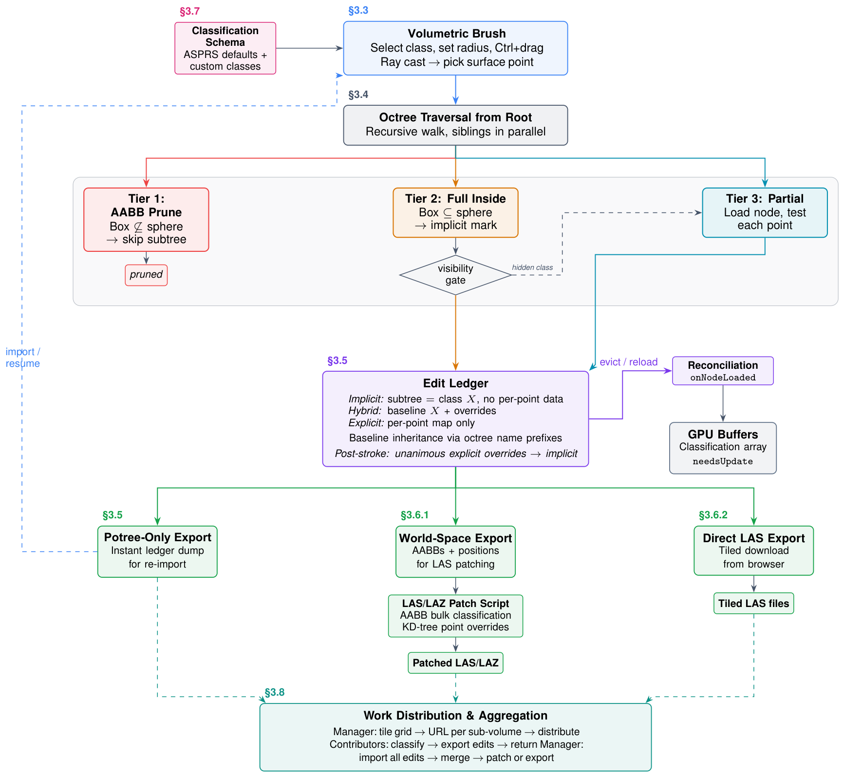
Figure 2.
Demonstration of the volumetric brush. Dataset: CyArk Ancient Corinth, distributed by Open Heritage 3D [59].
Figure 2.
Demonstration of the volumetric brush. Dataset: CyArk Ancient Corinth, distributed by Open Heritage 3D [59].
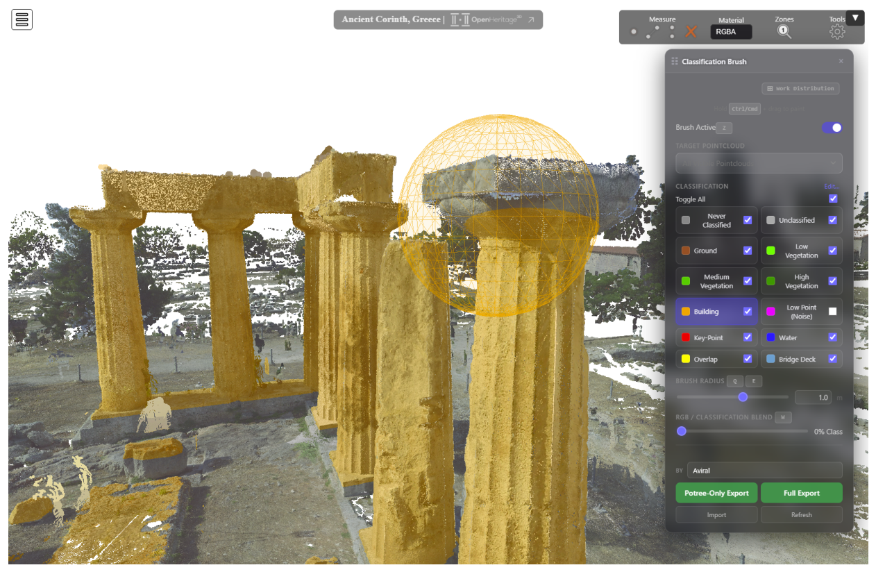
Figure 3.
(a) Classification result when evaluating currently loaded nodes only: sparse and incomplete selection; (b) Classification result when recursively classifying all intersected nodes: full coverage of brush-intersected points.
Figure 3.
(a) Classification result when evaluating currently loaded nodes only: sparse and incomplete selection; (b) Classification result when recursively classifying all intersected nodes: full coverage of brush-intersected points.
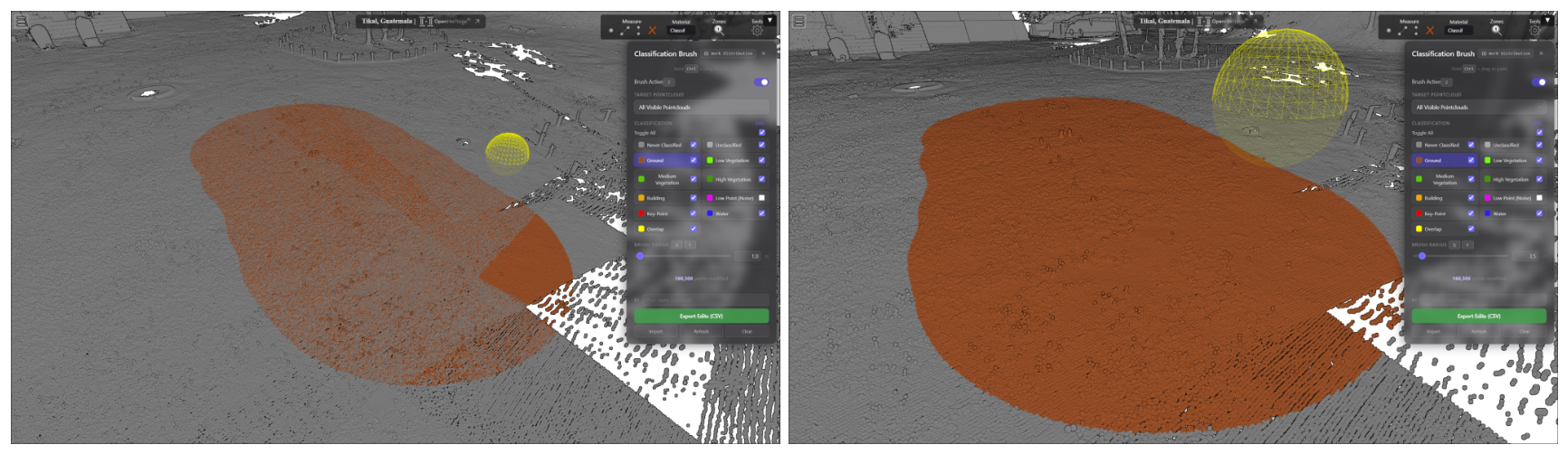
Figure 4.
Work distribution and aggregation workflow. A project manager subdivides a master clipping volume into an grid of sub-volumes, encodes each sub-volume as a viewer URL, and distributes the URLs to contributors. Each contributor classifies points within their assigned sub-volume and returns a ledger file, which the project manager imports, reviews for outliers and spatial overlap, and merges into a single classified dataset, either by patching the original LAS/LAZ files (Section 3.6.1) or by re-exporting from the viewer (Section 3.6.2).
Figure 4.
Work distribution and aggregation workflow. A project manager subdivides a master clipping volume into an grid of sub-volumes, encodes each sub-volume as a viewer URL, and distributes the URLs to contributors. Each contributor classifies points within their assigned sub-volume and returns a ledger file, which the project manager imports, reviews for outliers and spatial overlap, and merges into a single classified dataset, either by patching the original LAS/LAZ files (Section 3.6.1) or by re-exporting from the viewer (Section 3.6.2).
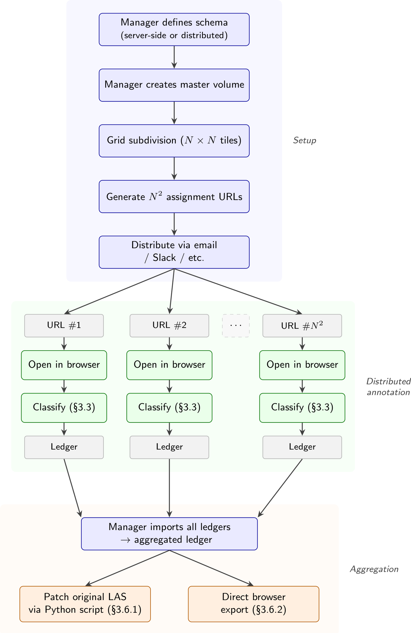
Figure 5.
Classification of the Pantheon portico. (a) Pure classification view showing eight semantic classes assigned to the facade. (b) Composite rendering mode blending RGB color with the classification overlay; surface detail including the dedicatory inscription remains legible through the tint. Dataset: Bern Digital Pantheon, distributed by Open Heritage 3D [63].
Figure 5.
Classification of the Pantheon portico. (a) Pure classification view showing eight semantic classes assigned to the facade. (b) Composite rendering mode blending RGB color with the classification overlay; surface detail including the dedicatory inscription remains legible through the tint. Dataset: Bern Digital Pantheon, distributed by Open Heritage 3D [63].
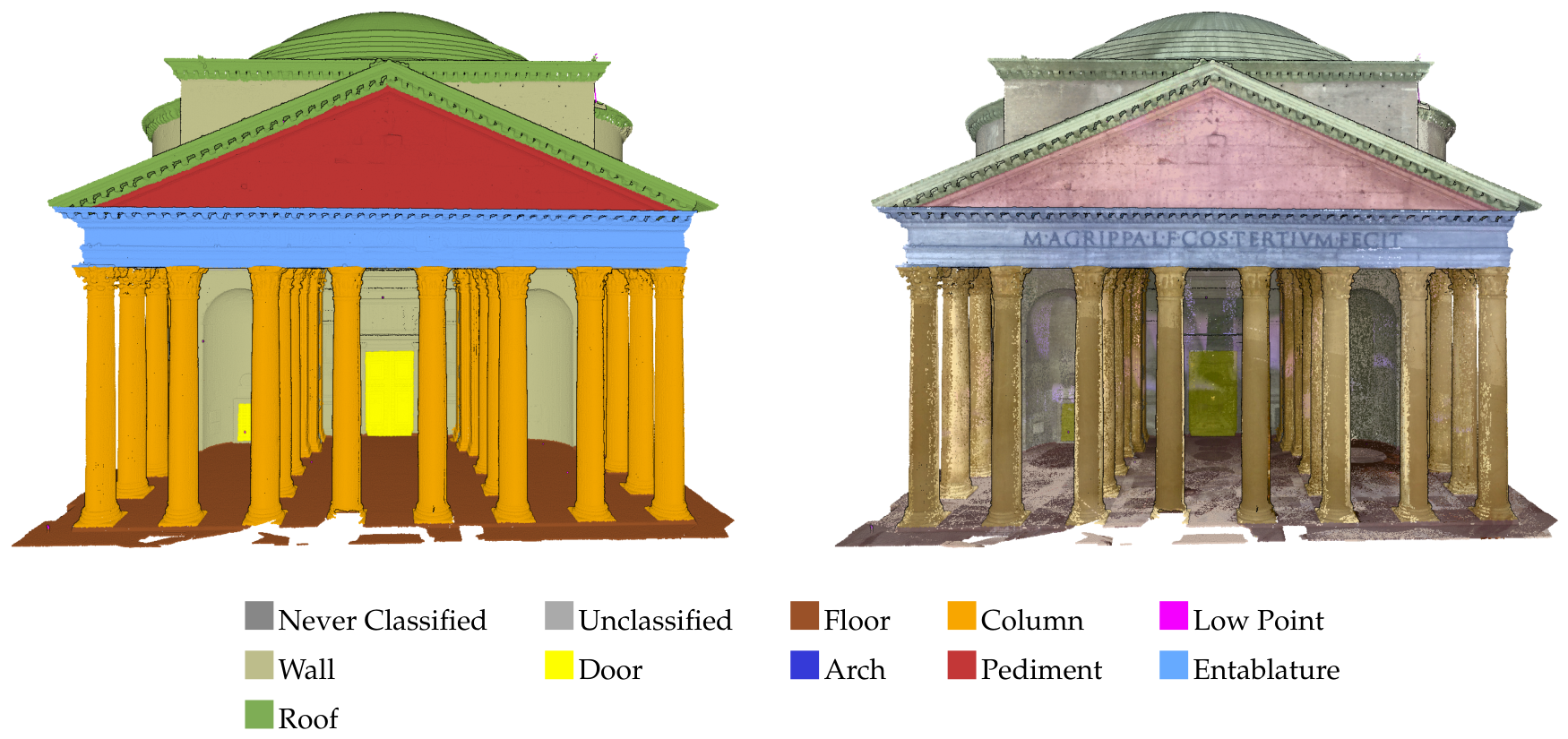
| Never Classified | Unclassified | Floor | Column | Low Point | |||||
| Wall | Door | Arch | Pediment | Entablature | |||||
| Roof |
Figure 6.
Aerial LiDAR change map of Castellammare neighborhood, with lost houses in red and lost vegetation in green (a) and close up showing mixed pixel error fringes left by differencing (b). Dataset: Palisades Fire 2025, distributed by ALERTCalifornia [64]
Figure 6.
Aerial LiDAR change map of Castellammare neighborhood, with lost houses in red and lost vegetation in green (a) and close up showing mixed pixel error fringes left by differencing (b). Dataset: Palisades Fire 2025, distributed by ALERTCalifornia [64]
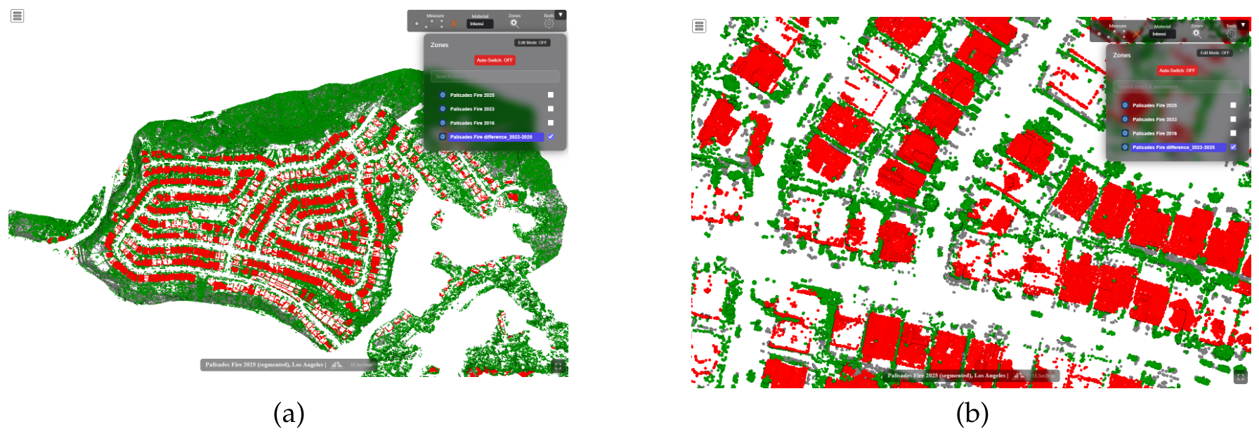
Figure 7.
Multi-contributor classification of the FR38 reef plot, Palmyra Atoll. (a) Work Distribution grid subdividing the master volume into nine tiles (A1–C3), each encoded as a viewer URL and assigned to one contributor. (b) The merged classification after importing all nine ledger files. Dataset distributed by OpenOcean3D [67].
Figure 7.
Multi-contributor classification of the FR38 reef plot, Palmyra Atoll. (a) Work Distribution grid subdividing the master volume into nine tiles (A1–C3), each encoded as a viewer URL and assigned to one contributor. (b) The merged classification after importing all nine ledger files. Dataset distributed by OpenOcean3D [67].
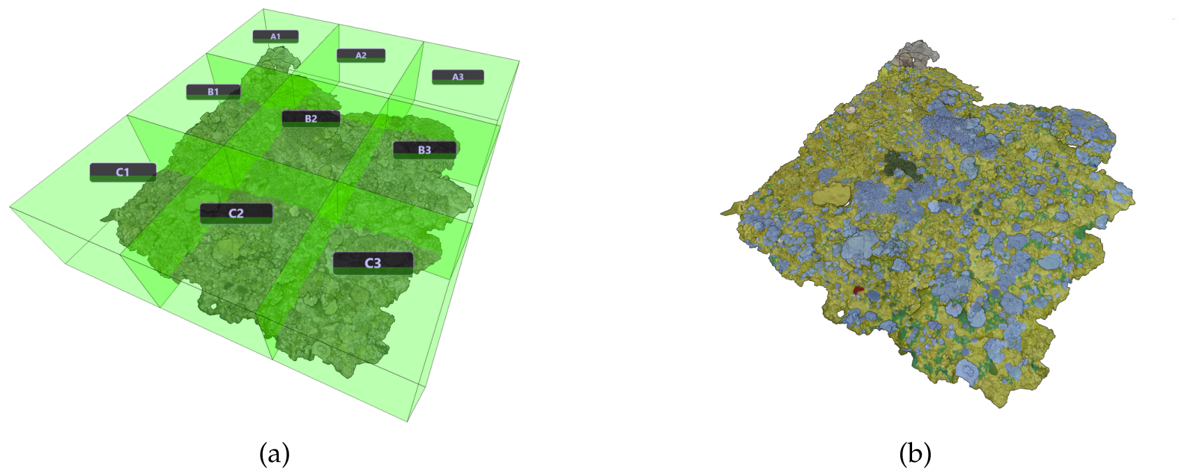
Figure 8.
Tile B2 before (a) and after (b) classification. The tile was bulk-assigned to substrate and the coral and algae classes were painted over that base with the volumetric brush.
Figure 8.
Tile B2 before (a) and after (b) classification. The tile was bulk-assigned to substrate and the coral and algae classes were painted over that base with the volumetric brush.
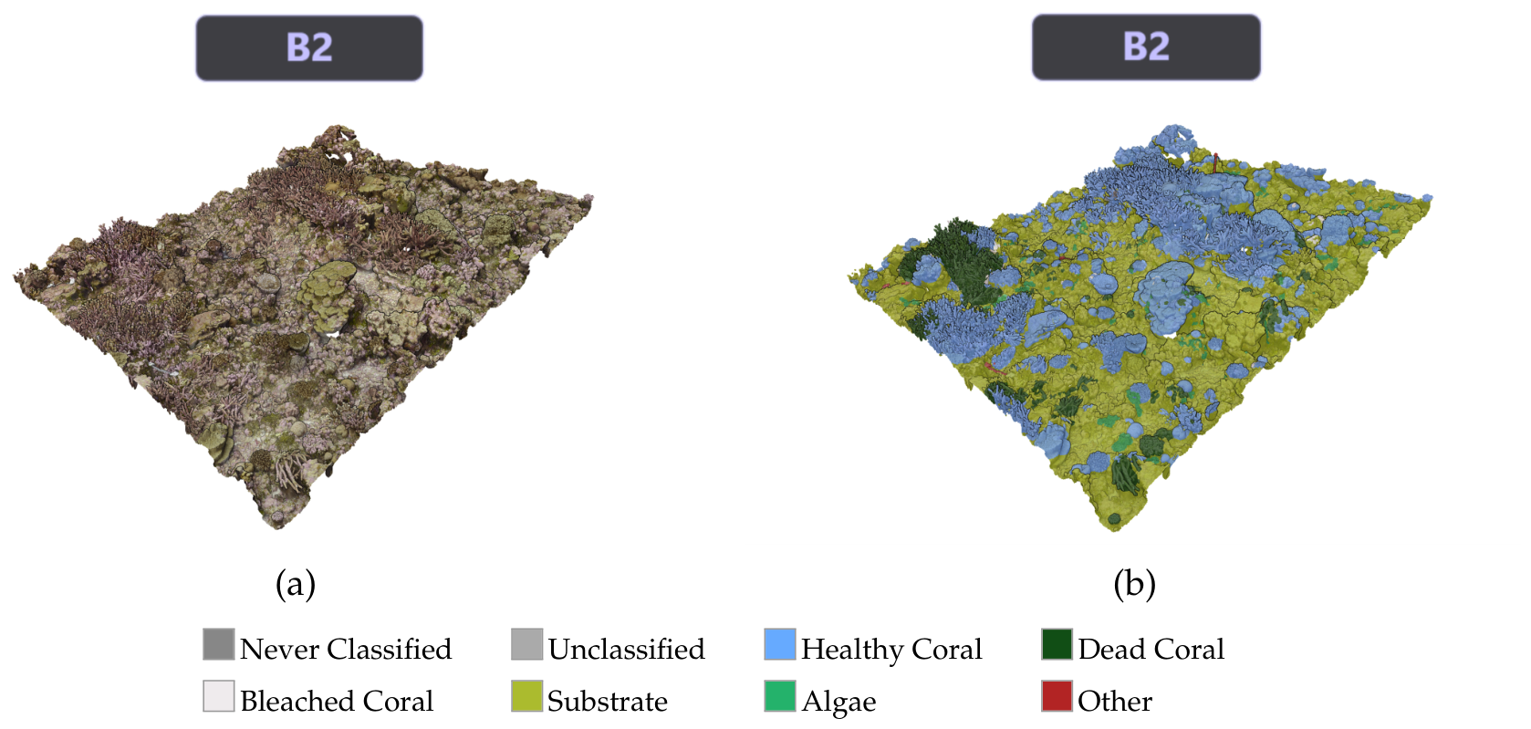
| Never Classified | Unclassified | Healthy Coral | Dead Coral | ||||
| Bleached Coral | Substrate | Algae | Other |
Figure 9.
Annotation with an oriented survey photograph focused. The camera is locked to the photograph’s pose so image and point cloud remain aligned; the surrounding cloud is rendered in pure classification color, and brush strokes applied through the photograph classify the underlying points.
Figure 9.
Annotation with an oriented survey photograph focused. The camera is locked to the photograph’s pose so image and point cloud remain aligned; the surrounding cloud is rendered in pure classification color, and brush strokes applied through the photograph classify the underlying points.
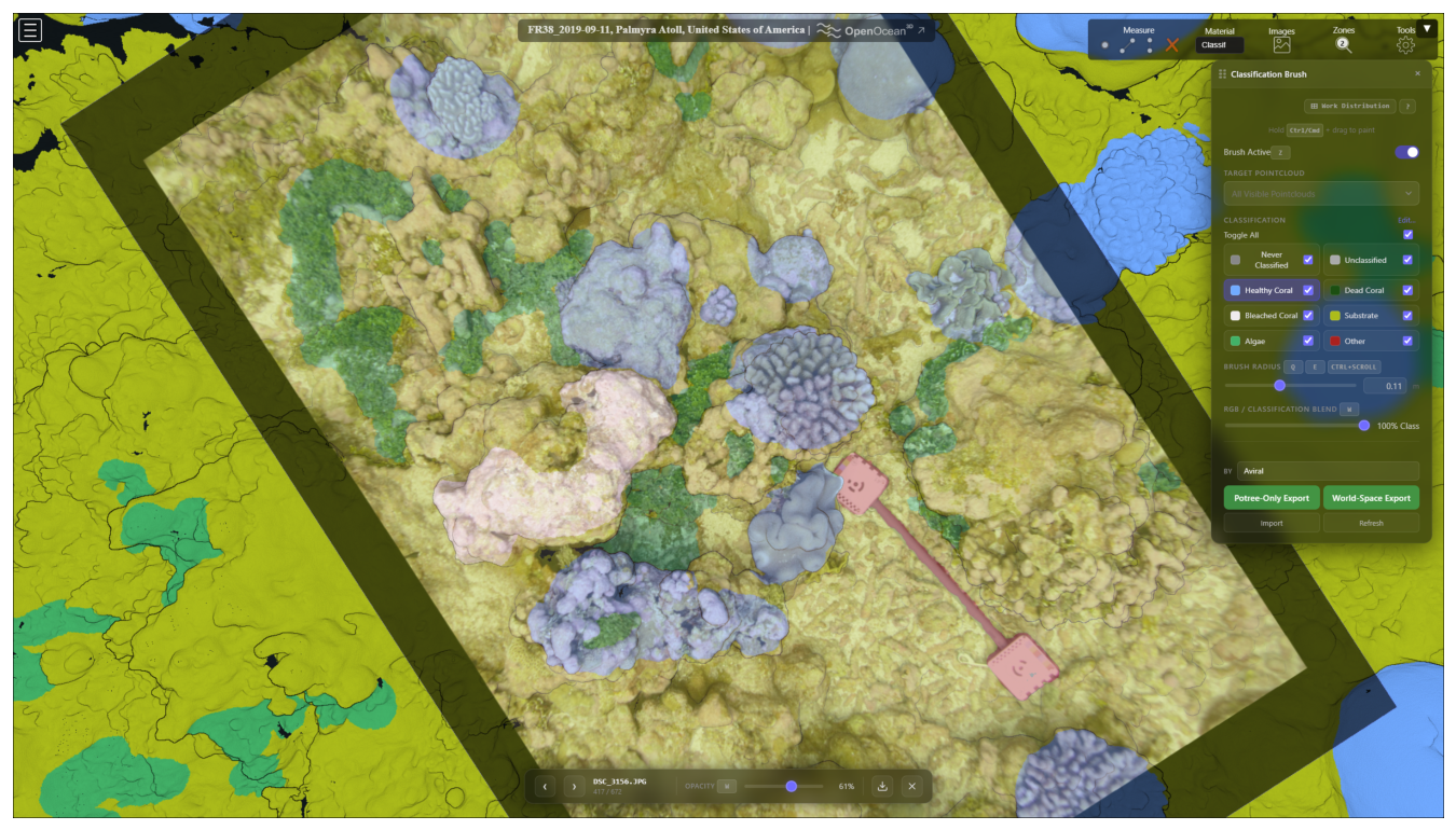
Figure 10.
The brush sphere (green) against the octree at the four radii of Table 2, shown at different scales. Yellow boxes are the bounding boxes of the nodes the viewer is currently displaying, not the nodes the stroke inspected. (a) m (): the sphere is smaller than the leaf node containing its center. (b) m (): the sphere spans many leaf nodes. (c) m (): leaf nodes are too small to resolve at this scale. (d) m (): the sphere encloses the octree root, and with it the entire plot.
Figure 10.
The brush sphere (green) against the octree at the four radii of Table 2, shown at different scales. Yellow boxes are the bounding boxes of the nodes the viewer is currently displaying, not the nodes the stroke inspected. (a) m (): the sphere is smaller than the leaf node containing its center. (b) m (): the sphere spans many leaf nodes. (c) m (): leaf nodes are too small to resolve at this scale. (d) m (): the sphere encloses the octree root, and with it the entire plot.
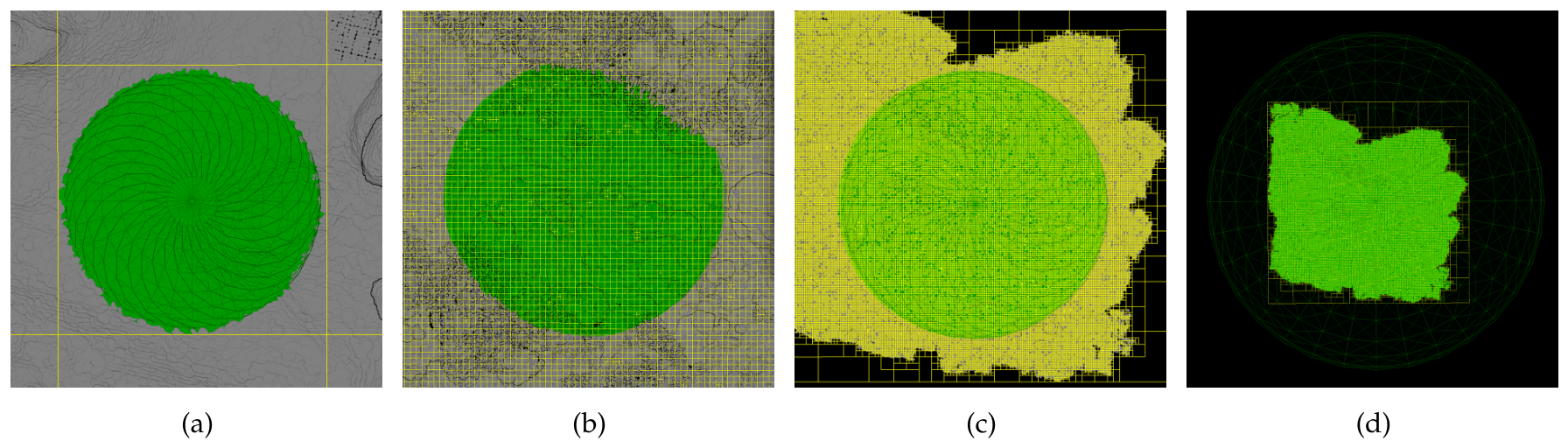
Table 1.
Distribution of the merged FR38 classification across ledger tiers. Explicit overrides are points recorded individually; the remainder of each class is assigned by implicit or hybrid baselines.
Table 1.
Distribution of the merged FR38 classification across ledger tiers. Explicit overrides are points recorded individually; the remainder of each class is assigned by implicit or hybrid baselines.
| Class | Code | Points | Share | Explicit overrides | Explicit share |
|---|---|---|---|---|---|
| Substrate | 67 | 287,026,102 | 63.0% | 1,425 | <0.001% |
| Healthy coral | 64 | 138,133,422 | 30.3% | 57,377,837 | 41.5% |
| Algae | 68 | 18,487,688 | 4.1% | 16,656,487 | 90.1% |
| Dead coral | 65 | 10,007,464 | 2.2% | 5,165,483 | 51.6% |
| Bleached coral | 66 | 1,684,464 | 0.4% | 1,025,603 | 60.9% |
| Other | 69 | 230,858 | 0.05% | 183,332 | 79.4% |
| Never classified | 0 | 103,462 | 0.02% | — | — |
Table 2.
Per-stroke node counts on the FR38 reef plot for a single brush center at four brush radii r; m is the edge length of the deepest node containing the center. Naive: nodes whose bounding box intersects the brush sphere, all of which the naive traversal loads and inspects. Inspected: nodes the tiered traversal loads and tests per point (third tier). Implicit: nodes recorded as implicit marks (second tier); neither they nor their descendants are loaded. Reduction: . Implicit share: percentage of the points classified by the stroke that are assigned by implicit marks rather than per-point overrides. At m the sphere encloses the octree root and with it the entire plot.
Table 2.
Per-stroke node counts on the FR38 reef plot for a single brush center at four brush radii r; m is the edge length of the deepest node containing the center. Naive: nodes whose bounding box intersects the brush sphere, all of which the naive traversal loads and inspects. Inspected: nodes the tiered traversal loads and tests per point (third tier). Implicit: nodes recorded as implicit marks (second tier); neither they nor their descendants are loaded. Reduction: . Implicit share: percentage of the points classified by the stroke that are assigned by implicit marks rather than per-point overrides. At m the sphere encloses the octree root and with it the entire plot.
| Nodes | Points | |||||
|---|---|---|---|---|---|---|
| r (m) | Naive | Inspected | Implicit | Reduction | Implicit share | |
| 0.04 | 0.48 | 12 | 12 | 0 | 0% | 0% |
| 2 | 23.9 | 6,355 | 1,114 | 501 | 82.5% | 85.5% |
| 7.2 | 85.6 | 75,970 | 3,003 | 1,609 | 96.0% | 96.7% |
| 30 | 358 | 147,905 | 0 | 1 | 100% | 100% |
Disclaimer/Publisher’s Note: The statements, opinions and data contained in all publications are solely those of the individual author(s) and contributor(s) and not of MDPI and/or the editor(s). MDPI and/or the editor(s) disclaim responsibility for any injury to people or property resulting from any ideas, methods, instructions or products referred to in the content. |
© 2026 by the authors. Licensee MDPI, Basel, Switzerland. This article is an open access article distributed under the terms and conditions of the Creative Commons Attribution (CC BY) license (http://creativecommons.org/licenses/by/4.0/).
Copyright: This open access article is published under a Creative Commons CC BY 4.0 license, which permit the free download, distribution, and reuse, provided that the author and preprint are cited in any reuse.