

Submitted:
02 October 2026
Posted:
05 October 2026
You are already at the latest version
Abstract
Arterial oxygen saturation measured by co-oximetry (SaO2m) is the clinical reference for oxygenation, but in the mechanically ventilated patients studied here the freshest usable value is nine hours old. We build a virtual sensor that bridges this gap from continuously recorded ventilator and gas-rig time series with gradient-boosted trees, and report it as three nested implementation scenarios of one code base: X0 (XGBoost 2.1.4 through our pipeline, no physics term active), XP (X0 plus a blend toward the anchor and the cumulative oxygen uptake rate over the gap per kilogram of body mass, derived from an oxygen balance of the arterial blood) and v4 (XP plus a patient-level anchor that recalibrates the nine-hour-old measurement toward the patient’s own history). Out-of-fold predictions under patient-grouped five-fold cross-validation are scored on the 3730 hours of 30 patients whose inputs contain no SaO2m value younger than nine hours. From X0 to XP, the mean per-patient MAPE decreases slightly, from 3.321% to 3.289%, an effect resolved by a paired patient bootstrap for this summary only. From XP to v4, it decreases further to 3.117%, the pooled MAPE decreases from 3.890% to 3.727% (both changes resolved by the bootstrap), and the pooled correlation increases from 0.754 to 0.793. Meanwhile, the model becomes substantially smaller, with the number of input features decreasing from 55 to 19 and the number of tree leaves decreasing from 9527 to 450. An exact decomposition of every prediction shows that in v4 the two-coefficient anchor earns 81% of the improvement over persistence and carries nearly all of the prediction variance. All formulas are matched line by line to the C++ and Python sources.
Keywords:
virtual sensor
; soft sensor
; gradient boosting
; XGBoost
; physics-informed machine learning
; mechanical ventilation
; oxygen saturation
; multivariate time series
; explainability
; patient-level calibration
1. Introduction
Effective critical care depends on having timely and accurate knowledge of the patient’s physiological state, yet intensive care units operate under persistent structural constraints that systematically undermine this requirement [1]. High patient to nurse ratios, equipment saturation during surge periods, and the physical impossibility of continuous bedside observation for every admitted patient mean that clinically significant changes in physiology can go undetected for extended periods [2]. Laboratory based measurements remain the clinical standard for several critical physiological variables, including cardiac output [3] or arterial oxygen saturation via co-oximetry [4,5], yet when the samples of intensive-care patients are analysed in a central laboratory the median turnaround time between blood collection and result availability is 56 minutes, so that in practice some clinical decisions are grounded in delayed information [6].
This growing divergence between the current state and the most recent measurement is not an edge case but a structural property of any monitoring system that relies on intermittent invasive sampling [7,8]. Retrospective analyses of large ICU databases have documented that missing or delayed values in key physiological variables are systematically associated with suboptimal alarm management and delayed recognition of clinical deterioration [7,9]. For patients receiving mechanical ventilation, however, a continuously available high-resolution data source already exists: the ventilator itself, which continuously records a rich stream of respiratory signals that reflect the patient’s respiratory mechanics and gas-exchange capacity in real time [2,10]. The predictive value of this stream has already been established for within-ventilator prediction tasks, Qiu et al. [11] demonstrated that a long short-term memory relation network trained on MIMIC-III can predict patient-specific ventilator parameters in real time. If ventilator signals are sufficiently informative to predict future ventilator parameters, they should also carry information relevant to predicting other physiological variables, such as , as demonstrated by prior work linking ventilator settings to patient oxygenation outcomes [12,13]. This follows the soft-sensor paradigm, where continuously available signals are used to estimate intermittently measured variables [14].
Recent advances in soft sensing have shown that capturing long-range temporal structure is essential, [14] propose a temporal convolutional network with both spatial and temporal attention mechanisms, showing that temporally aware models are preferred for such task.
In the medical domain, the soft-sensor paradigm has been successfully applied across a broad range of continuous physiological estimation problems, establishing a strong precedent for the clinical feasibility of the approach [15]. Beyond oxygenation-related variables, soft-sensor approaches have been successfully explored for glucose monitoring, cardiovascular assessment, respiratory monitoring, intracranial pressure estimation, and wearable health applications, consistently demonstrating the potential of machine-learning models to infer clinically relevant physiological states from routinely collected signals [4,16,17,18,19,20,21,22,23].
Recent work in ICU time-series modeling emphasizes the importance of explicitly representing temporal dynamics under irregular sampling. Lee et al. [8,24] show that incorporating inter-event time gaps into recurrent architectures improves predictive performance by allowing models to exploit temporal spacing as an informative signal rather than treating it as missingness. Similarly, adaptive recurrent formulations that condition hidden state updates on elapsed time further improve modeling of heterogeneous physiological trajectories in critical care settings [25]. Patharkar et al. [7] summarize these findings across biomedical time-series applications, highlighting that methods accounting for irregular sampling consistently outperform standard sequence models.
Among physiological targets in critical care, oxygenation estimation has received growing attention, yet existing approaches leave the core problem of this study unresolved. Woo et al. [26] trained Random Forest and XGBoost models on a large-scale multi-centre ICU dataset to predict from and clinical covariates, reducing estimation error substantially over the pulse oximetry baseline, but the approach corrects an available signal rather than operating in its absence. Cabanas et al. [27] further highlight the regulatory and technical limitations of AI-enhanced pulse oximetry, reinforcing that -dependent correction methods have fundamental constraints in failure scenarios.
The closest line of work to ours estimates oxygenation directly from ventilator signals without relying on pulse oximetry. Where Ghazal et al. [28] trained a bootstrap-aggregated decision tree to predict categories five minutes after a ventilator setting change, achieving an AUC below 0.75 a result that also reveals the core limitation: a five-minute classification horizon is far too narrow to address the multi-hour sensor-absence scenario we target. Dong et al. [5] take a closer approach, using a non-linear additive model to estimate blood gas pH and between invasive draws from ventilator-derived inputs, achieving clinically acceptable accuracy, but their target variable is not and the gap length is never varied or evaluated as a modeling parameter. Hser et al. [29] incorporate oxygenation estimation within a broader ICU respiratory monitoring system using gradient boosted models, predicting respiratory failure events up to ten hours ahead, but their estimator still takes as a continuous input, making it inapplicable when pulse oximetry is unavailable. Finally, Si et al. [30] estimate from facial video using Random Forest and Support Vector Regression, demonstrating non-contact sensing potential but under controlled low-acuity conditions incompatible with the mechanically ventilated ICU patient.
Across these works, three gaps remain open: no approach models prediction accuracy as a function of elapsed time since the last measurement, none operates without assuming availability, and none separates what a physical prior contributes from what the learned trees contribute under patient-level cross-validation. This paper addresses the three, building on the oxygen conservation law of our bioprocess soft sensors [31,32], on its transfer to human respiration [33,34], and on the maximum-relative-entropy weighting of our earlier estimators [32,35,36]. It bridges a nine-hour absence of the co-oximetry measurement from ventilator and gas-rig time series with gradient-boosted trees; it works without pulse oximetry; and it is reported as three explicit implementation scenarios of one code base, the unmodified library through our pipeline (X0), the library with our anchor blend and the cumulative oxygen uptake rate over the gap (XP), and the latter with a patient-level calibrated anchor (v4), so that every improvement is attributed to the code that produced it, every equation is matched to the line that implements it, and an exact decomposition of each prediction says how much of it is physics and how much is trees. The rest of the paper is organized as follows: Section 2 describes the data, the three scenarios, the shared boosted ensemble with a numeric trace of its leaves, the physics-informed terms with their derivations and code, and the evaluation protocol; Section 3 reports the three scenarios on identical folds, the anchor coefficients, the anatomy of the predictions and the ablations; Section 4 and Section 5 discuss and conclude.
2. Materials and Methods
The objective of this study is to predict , the arterial oxygen saturation measured by co-oximetry, from hourly processed clinical variables, respiratory parameters and experimental gas-rig transducers, nine hours after the last available measurement. A principal characteristic of the study is the translation of soft-sensor technologies from bioprocess engineering to human physiological monitoring: as demonstrated by Kemesis et al. [34], industrial off-gas sensors can be adapted to the non-invasive continuous tracking of human respiratory gas exchange.
We define the dataset as the matrix , where is the number of hourly samples and is the number of features that the boosted trees receive (its value depends on the scenario, Section 2.2), and the i-th row is the feature vector of the i-th sample. The target vector is , the values of every patient-hour. The mapping is
where is the predicted of the i-th sample and is a regressor with learned parameters . Three implementations of are compared in this paper; they share one code base and differ in which of our additions are active.
2.1. Dataset and Preprocessing
The study cohort comprises mechanically ventilated patients, totaling recorded hourly entries. Of these, hours have a measured target; all of them are predicted out of fold under five-fold patient-grouped cross-validation, and the results are reported on the hours of 30 patients whose inputs contain no value younger than nine hours (Section 3.7), with the values on all hours listed alongside. In 322 patient-hours (644 rows, five patients) two blood gas measurements were documented within the same nominal hour. These rows are retained in the reported numbers; a sensitivity analysis keeping only the last measurement per hour is reported in Section 3.1.
The target variable is discrete and integer-valued, spanning 73 distinct levels from to (median , 1st percentile ; 350 observations fall below , and a single observation exceeding was retained as an authentic clinical recording). This discrete distribution is directly relevant to the mechanics of the persistence baseline (Section 3.6). All features entering the decision trees were standardized using Z-score normalization fitted strictly on the training folds; in contrast, all physiological quantities supplied directly to the analytical anchor (Section 2.4) were preserved in their raw, natural physical units.
Figure 1.
Temporal problem formulation and prediction horizon. The model estimates the current oxygenation state by bridging a nine-hour absence of the co-oximetry measurement. The last available measurements and supply the physiological baseline; the continuous ventilator and gas-sensor channels supply the real-time information available at hour t.
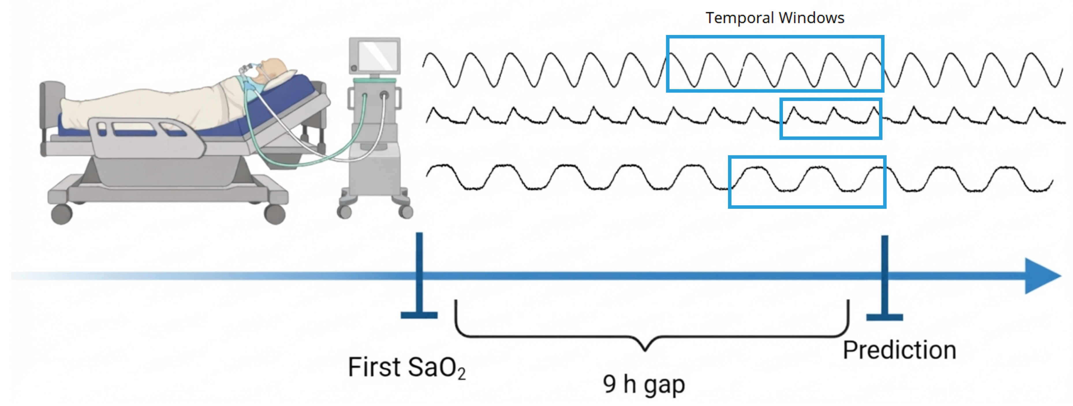
We define a prediction horizon of nine hours. The history at and hours is included to establish the patient’s baseline prior to the simulated sensor gap, ensuring the model remains grounded in the patient’s physiological state without using future information. More precisely, the feature value provided at hour t represents the most recent observation recorded at or before. Consequently, the actual elapsed time since that baseline reading was taken is at least nine hours and varies depending on clinical sampling irregularity; its empirical distribution is analyzed in Section 3.6.
2.1.1. Signals and Their Lags in Each Scenario
Six real-time signals are engineered from the ventilator and the gas rig and lagged; three target-derived and two static descriptors complete the input. Table 1 lists the six signals with the lag hours that each scenario builds and, of those, the ones the trees are allowed to see. Table 2 lists the remaining columns. The counts differ between the scenarios: the trees of X0 and XP receive columns (six signals at hour t, their 44 lagged copies, and the five columns of Table 2 that are tree inputs), whereas the trees of v4 receive (five signals at t with two lags each, plus four of those five columns). In v4 the pruning of the lag lists was decided by tolerance tests on the out-of-fold macro MAPE (Section 3); the signal O2diffxPower (a signal which is proportional to Oxygen Uptake Rate, OUR) is hidden from the trees in v4 because it feeds the physics terms instead.

Table 1.
Dynamic signals and their lag hours. Each cell lists the hours t and at which the signal enters the data as a column (data_preparation.py); the count in brackets is the number of such columns. In X0 and XP every column is a tree input. For O2diffxPower the listed hours are also the sampling hours of the cumulative oxygen uptake rate, Eq. (16): the available values at these hours are averaged and the average is multiplied by the gap D and divided by the body mass; in v4 these columns serve only that purpose and are not tree inputs. O2conc: inspired O2 concentration at the mask inlet (%). GM102B_Volts: electrochemical gas-sensor output voltage (V). CO2xPower: expired CO2 concentration times the ventilator power integral. O2xPress: O2conc times airway pressure. O2xPressplusPEEP: O2conc times pressure plus PEEP, a delivery composite. O2diffxPower: inlet-minus-expiratory O2 concentration times the power integral, proportional to the oxygen uptake rate; it is the oxygen uptake rate signal of Section 2.4.
| Signal | Hours in X0 and XP (all tree inputs) | Hours in v4 | Of these, tree inputs in v4 |
|---|---|---|---|
| O2conc | t, (6 cols) | t, | t, (3 cols) |
| GM102B_Volts | t, (8 cols) | t, | t, (3 cols) |
| CO2xPower | t, (6 cols) | t, | t, (3 cols) |
| O2xPress | t, (10 cols) | t, | t, (3 cols) |
| O2xPressplusPEEP | t, (11 cols) | t, | t, (3 cols) |
| O2diffxPower | t, (9 cols; also the sampling hours of Eq. (16) in XP) | t, (the sampling hours of Eq. (16)) | none |
| tree inputs from this table: 50 | 15 | ||
Table 2.
Target-derived and static columns. "Tree" says whether the boosted trees receive the column in that scenario; "anchor" says whether the column feeds the anchor of Section 2.4 instead. runmean_SaO2m exists only in v4.
Table 2.
Target-derived and static columns. "Tree" says whether the boosted trees receive the column in that scenario; "anchor" says whether the column feeds the anchor of Section 2.4 instead. runmean_SaO2m exists only in v4.
| Column | Description | X0, XP | v4 |
|---|---|---|---|
| SaO2m_lag_9h | most recent measured at or before h (%); the persistence value of Eq. (17) | tree and anchor | tree and anchor |
| SaO2m_lag_10h | most recent measured at or before h (%) | tree | tree |
| SaO2m_first | the patient’s first measurement (%) | tree | tree |
| runmean_SaO2m | mean of all measurements at or before h, Eq. (20) | not built | anchor only |
| count_hours | elapsed treatment time (h) | tree | tree |
| Svoris | body mass (kg); also normalises the cumulative OUR term | tree | anchor scale only |
| tree inputs from this table | 5 | 4 | |
| total tree inputs | 55 | 19 | |
2.2. Three Implementation Scenarios
Every number in this paper is attributed to one of three scenarios of one code base (Python pipeline and a patched XGBoost 2.1.4 C++ library). They are nested: each adds to the previous one and changes nothing else.
- X0—XGBoost. The XGBoost 2.1.4 library, trained by our Python pipeline with the tree inputs of Table 1Table 2 (), the initial prediction equal to the persistence value , the cost-sensitive weights of Section 2.3, and the hyper-parameters of Table 8. The two C++ terms added for XP are compiled into the library used here as well, but both coefficients are zero ( in Eq. (37)), which makes them identities: X0 produces what unmodified XGBoost 2.1.4 produces from the same pipeline, up to float32 rounding.
- XP — XGBoost with our anchor blend and cumulative OUR term. X0 plus the two C++ terms of Section 2.6 with their configured coefficients and : the final prediction is pulled toward the persistence value and receives the cumulative oxygen uptake rate over the gap per kilogram of body mass, Eq. (16). Same trees, same .
- v4 — XP with the patient-level calibrated anchor. XP plus the anchor of Section 2.4.5, which replaces the raw persistence value by a least-squares combination of the persistence value and the patient’s own measurement history, fitted on each training fold; its trees receive inputs and the hyperparameters of Table 9. , .
Every code excerpt and equation in this paper follows a unified typographical convention.
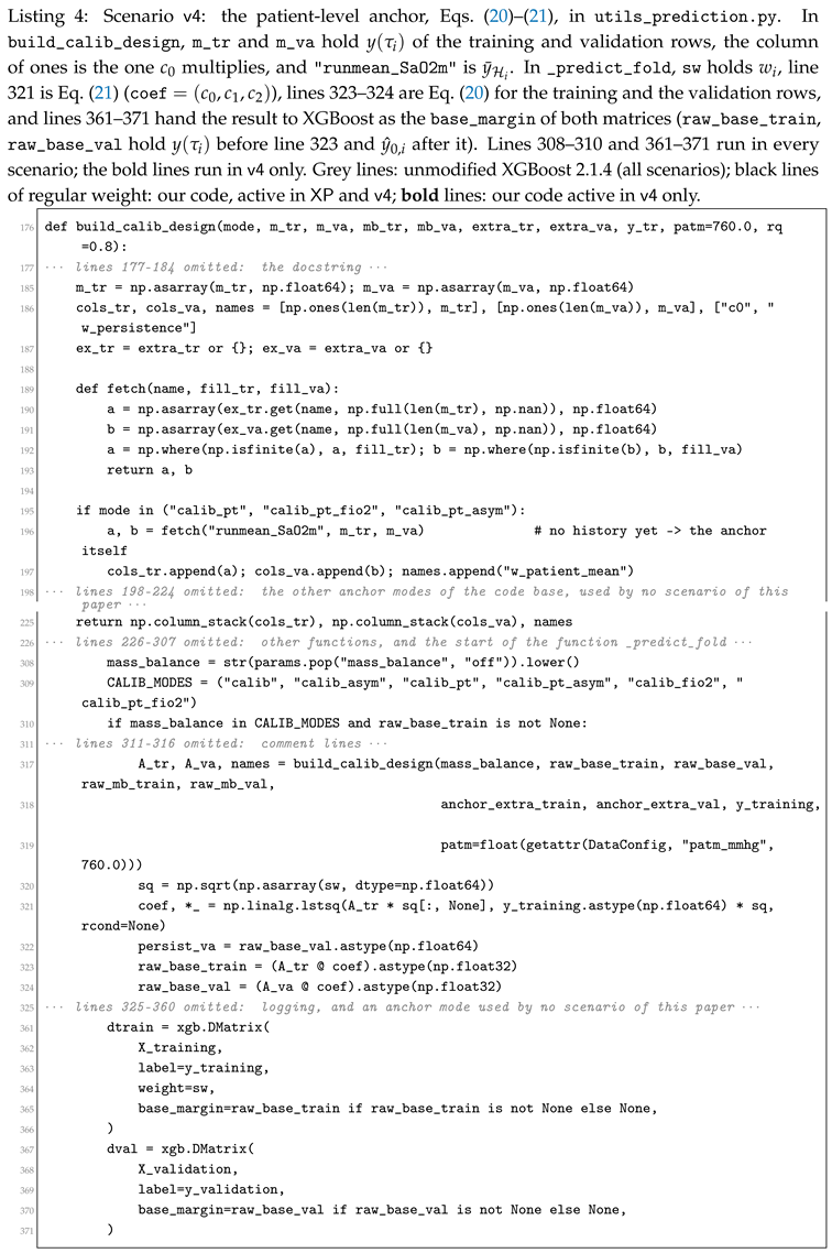
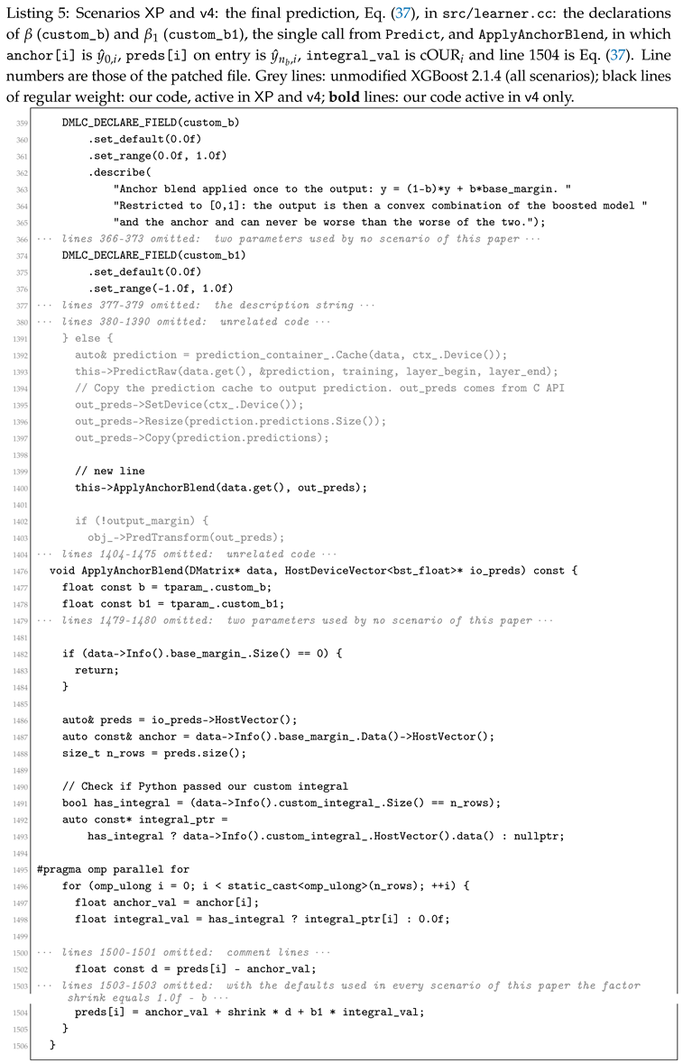
In code listings: dark gray denotes unmodified upstream XGBoost (v2.1.4) source code; regular black font indicates our additions active in both XP and v4 (our Python pipeline and C++ extensions); and bold font denotes additions active exclusively in v4. Excerpts of original XGBoost source in Section 2.5 are therefore rendered entirely in gray.
In equations: our contributions carry the label [XP] if active in both XP and v4, and are set in bold with the label [v4] if unique to v4. Standard equations from baseline XGBoost or established physiological literature remain unmarked. Table 3 lists every mathematical symbol with its unit and corresponding code variable.
2.3. The Loss: Cost-Sensitive Sample Weights and the Relative-Entropy Criterion
Two fits in this paper minimise a weighted sum of squared errors over the training rows: the least-squares fit of the patient-level anchor of v4 (Section 2.4.5) and the boosted trees of all three scenarios (Section 2.5). Both use one dimensionless weight per row,
where is the target in %, is a dimensionless floor (custom_kp), a dimensionless exponent (custom_power) and a stabiliser in (custom_eps); the three are fields of config.py, class TrainConfig, and the weights are the array sw computed by compute_sample_weights (utils_prediction.py). The weights are the same in the three scenarios up to the values of and (Table 8 and Table 9).
The family (2) descends from our maximum-relative-entropy estimators [31,32,35], where it was written for the biomass concentration of a cultivation with a fixed square in place of the exponent , and its single coefficient was named ; in the notation of this paper that coefficient is and the observed quantity is . For a Gaussian density of the prediction and a Gaussian likelihood centred on the observation with variance (in ), the relative entropy of row i is [32]
dimensionless, with the variance model [32]
in which is a constant scale in , enters with its numerical value in %, and gives the printed form of the cited papers. Inserting Eq. (4) into Eq. (3) and summing over the training rows gives
whose bracket is Eq. (2) with . The weighted squared loss used below is therefore the relative-entropy criterion of [32], generalised by the exponent and the stabiliser [36]; is the single coefficient that trades the error relative to (the MAPE end, ) against the squared error (the variance end, ). Its measured effect on this cohort is given in Section 3.5.
Table 3.
Symbols, units and names in the code (dp: data_preparation.py; up: utils_prediction.py; lc: src/learner.cc). a.u.: arbitrary units of the gas signals.
Table 3.
Symbols, units and names in the code (dp: data_preparation.py; up: utils_prediction.py; lc: src/learner.cc). a.u.: arbitrary units of the gas signals.
| Symbol | Meaning | Unit | Name in the code |
|---|---|---|---|
| i, | row (one patient-hour), number of rows | — | row of the data frame |
| , | patient of row i, number of patients | — | patient_id |
| hour of row i | h | LocalTime | |
| measured , the target | % | SaO2m | |
| D | nominal gap | h | virtual_sensor_gap |
| , | time and age of the last measurement available at , Eq. (17) | h | inside _time_based_lag_last_known (dp) |
| last available measurement | % | SaO2m_lag_9h; raw_lag_tr, raw_lag_va (up) | |
| ; | measurement times available at ; mean of y over them, Eq. (20) | h; % | runmean_SaO2m |
| body mass | kg | Svoris | |
| oxygen uptake rate signal at the airway | a.u. | O2diffxPower | |
| carbon dioxide production rate signal | a.u. | CO2xPower | |
| , | coefficients of the balance, Eq. (13) | % kg h−1 a.u.−1 | — |
| lag set of the OUR signal | h | lags of O2diffxPower | |
| cumulative oxygen uptake rate over the gap per kg, Eq. (16) | a.u. h kg−1 | integral_O2diffxPower; field custom_integral | |
| initial prediction, the anchor | % | raw_base_train, raw_base_val; base_margin; anchor (lc) | |
| ; , | coefficients of the patient-level anchor, Eq. (20) | %; — | coef[0]; coef[1], coef[2] (up) |
| sample weight, Eq. (2) | — | sw | |
| ; ; | floor, exponent and stabiliser of , Eq. (2) | —; —; | custom_kp, custom_power, custom_eps |
| b, | boosting round, number of trees | — | rounds of xgb.train |
| , | tree b, score of its leaf j | % | XGBoost internal |
| learning rate | — | learning_rate | |
| ; ; | L2, L1 and per-split penalties | —; %; | reg_lambda, reg_alpha, gamma |
| , | gradient and Hessian of row i in round b | %, — | XGBoost internal |
| ; | running and raw boosted prediction | % | prediction buffer; preds (lc) |
| final prediction, Eq. (37) | % | pred_val, pred_tr (up) | |
| ; | anchor blend; weight of | —; % kg h−1 a.u.−1 | custom_b, custom_b1 |
| ; , | precursor model: mass transfer capacity; maximal oxygen solubility | s−1; mmHg | — |
2.4. From the Oxygen Balance to the Physics-Informed Terms
This subsection derives, from the oxygen conservation law of our earlier work, the two terms that the scenarios add to the boosted trees of Section 2.5: the cumulative oxygen uptake rate of XP, Eq. (16), and the patient-level anchor of v4, Eq. (20). The derived columns integral_O2diffxPower and runmean_SaO2m are removed from the tree inputs (utils_prediction.py, _extract_base_margin) and reach the model only through these terms.
2.4.1. Precursors: the Oxygen Conservation Law of Our Earlier Work
In aerobic bioprocesses, at a stationary oxidative state the oxygen uptake rate of the culture, OUR, equals the oxygen transfer rate from the gas, OTR, both in amount of oxygen per unit volume and time [31,33]:
In the time domain the same conservation law reads [33,37]: the dissolved oxygen, written as its partial pressure (mmHg), accumulates by what is transferred minus what is taken up,
and the transfer is proportional to the distance from the maximal oxygen solubility (mmHg), with the oxygen mass transfer capacity (s−1) [33]:
Substituting Eq. (8) into Eq. (7) and replacing the dissolved oxygen of the nutritional medium by the partial pressure of oxygen in arterial blood, (mmHg), Survyla et al. [33] and Kemesis et al. [34] obtained the model of arterial oxygen they applied to a human volunteer and to ventilated children,
in which is the airway signal of their gas-analysis device and its calibration coefficient, so that is in mmHg s−1 (in [33], Table I: , s−1, mmHg for one volunteer). To use sampled data, Survyla et al. [33] integrated the balance between two neighbouring sample times and (s) and divided both sides by the interval , a bar denoting the average over the interval (their Eqs. (8)–(9)); applied to Eq. (9) this step gives
Integrating the rate before using it is also the idea of the cumulative oxygen uptake rate cOUR [31]: the integral of OUR is less noisy than OUR itself. Two features of Eq. (9) do not fit the present task. It is written for partial pressure, and in the trial of [33] the haemoglobin saturation did not change noticeably, so the dissociation curve played no role, whereas here the target is the saturation itself. And it needs and , which were identified per person from blood gases, whereas no per-patient calibration is available at prediction time here.
2.4.2. The Balance Used Here: Saturation, Whole-Body Amounts, Body Mass on the Left
Three physiological facts connect Eq. (7) to the saturation y (%). The oxygen content of arterial blood, (mL O2 per dL of blood), is carried almost entirely by haemoglobin, of concentration Hb (g/dL) [38]:
at Hb g/dL, and mmHg the dissolved term is against mL/dL bound to haemoglobin. The amount of oxygen in the circulating blood is the content times the blood volume (dL), and the blood volume is proportional to the body mass (kg), with dL/kg in adults [39]. Written for amounts instead of concentrations, Eq. (7) states that the oxygen held in the blood changes by the oxygen taken from the ventilator gas, (mL O2 h−1), which is what the airway signal measures (inspired minus expired oxygen times the gas flow [40]), minus the oxygen consumed by the tissues, which equals the carbon dioxide production (mL CO2 h−1) divided by the dimensionless respiratory quotient RQ. With body mass on the left:
Eq. (12) is the conservation law of Eq. (7), as is Eq. (9) and its sampled form Eq. (10); Table 4 lists how each term of Eq. (10) corresponds to a term of Eq. (12) and of its integrated form, Eq. (15) below. The difference is the closure. Eq. (10) models the transfer from the gradient, , and uses the airway signal as the uptake, the two being equal in the stationary state of Eq. (6). Eq. (12) takes the transfer into the blood from the airway signal, which is what that signal physically measures, and takes the tissue consumption from the CO2 production; it therefore needs neither nor .
Table 4.
Correspondence between the precursor balance, Eq. (10), and the balance of this paper, Eqs. (12) and (15).
| Role in the balance | Precursor, Eq. (10) | This paper, Eqs. (12), (15) |
|---|---|---|
| state variable | (mmHg), per unit volume | y (%) through , Eq. (11), whole body through |
| accumulation | change of over | change of y over the gap D |
| transfer into the blood | , modelled | , measured at the airway as |
| consumption | , from the airway signal | , from ; not used in the three scenarios () |
| time step | interval between two samples | gap h |
The assumptions are: (A1) the arterial blood is one well-mixed compartment whose volume does not change over the gap; (A2) Hb is constant over the gap and the dissolved term of Eq. (11) is neglected, so ; (A3) the airway signal , the column O2diffxPower (inlet-minus-expiratory O2 concentration times the ventilator power integral, in arbitrary units a.u.), is proportional to the oxygen taken from the gas, with in mL O2 h−1 a.u.−1, the power integral standing for the gas flow; (A4) the signal , the column CO2xPower (a.u.), is proportional to the CO2 production, with in mL CO2 h−1 a.u.−1, and RQ is constant over the gap; (A5) these constants are shared by the patients of a training fold; (A6) the hourly samples are missing at random. Substituting (A2)–(A4) into Eq. (12) and collecting the constants into and , both in % kg h−1 a.u.−1, gives the balance with body mass on the left,
and dividing both sides by ,
This is why the oxygen uptake signal enters the code per kilogram of body mass. In the three scenarios of this paper the consumption term of Eq. (14) is not used: its coefficient is zero there, and only the uptake term is carried from here on.
2.4.3. Integration over the Gap: the Cumulative Oxygen Uptake Rate
Integrating Eq. (14) over the gap , as Eq. (10) integrates between samples, with the hour of row i and h (config.py, virtual_sensor_gap):
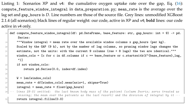
where is the last known body mass of the patient of row i (column Svoris; for a patient with no recorded mass the mean over the patients). The integral is the cumulative oxygen uptake rate of [31], taken over the gap and per kilogram. The code evaluates it with the rectangle rule from the OUR values recorded at the hours of the lag set (h), the lags of Table 1 plus the current hour ( in X0 and XP, in v4): the available values are summed, the sum is divided by their number (, the hours at which a value exists for row i), and the average is multiplied by the width D of the integration interval and divided by the body mass:
in a.u. h kg−1 (column integral_O2diffxPower, Listings 1 and 2; the mean over the available columns is mean(axis=1, skipna=True)). Under (A6) the sample mean is unbiased for the time average of over the gap, so Eq. (16) is unbiased for the integral [41]; the plain sum would equal times it and shrink with every missing hour. If is Lipschitz with constant (a.u. kg−1 h−1), the error of the rectangle rule on an hourly grid is at most [42]. The factor is the gap D and not the number of columns; the two coincide in X0 and XP when all nine values are present () but not in v4, and the factor D keeps the units when lags are pruned. Only the row’s own signals up to are used.
2.4.4. The Last Available Measurement
The measurement of y that the sensor may use at hour is the most recent one taken at or before :
where denotes the actual elapsed time (in hours). The term corresponds to the nine-hour lagged oxygen saturation (SaO2m_lag_9h), representing the most recent measurement recorded at or before . During the initial hours of an ICU admission before a nine-hour history is established (), this value defaults to the patient’s first recorded measurement. Substituting for and substituting Eq. (16) into Eq. (15) yields the integrated oxygen mass balance,
whose two terms the scenarios use as listed in Table 5. In X0 and XP the initial prediction of the boosted trees is the last available measurement itself,
so the trees learn corrections to the nine-hour-old measurement rather than to a constant.
Table 5.
How each scenario uses the terms of the integrated oxygen balance, Eq. (18).
Table 5.
How each scenario uses the terms of the integrated oxygen balance, Eq. (18).
| Term | X0 | XP | v4 |
|---|---|---|---|
| initial prediction, Eq. (19) | initial prediction, Eq. (19) | recalibrated toward the patient’s history, Eq. (20) | |
| not used | in Eq. (37), | in Eq. (37), |
is found by tuning, not by least squares, and in X0 and XP the trees also receive the OUR signal columns, so is not an estimate of ; both multiply the cumulative oxygen uptake per kilogram over the gap.
2.4.5. Scenario v4: the Patient-Level Anchor
Let be the times of all measurements of the patient available at ; the same information as uses, so no new leakage enters. In v4 the initial prediction recalibrates the last available measurement toward the patient’s own past mean:
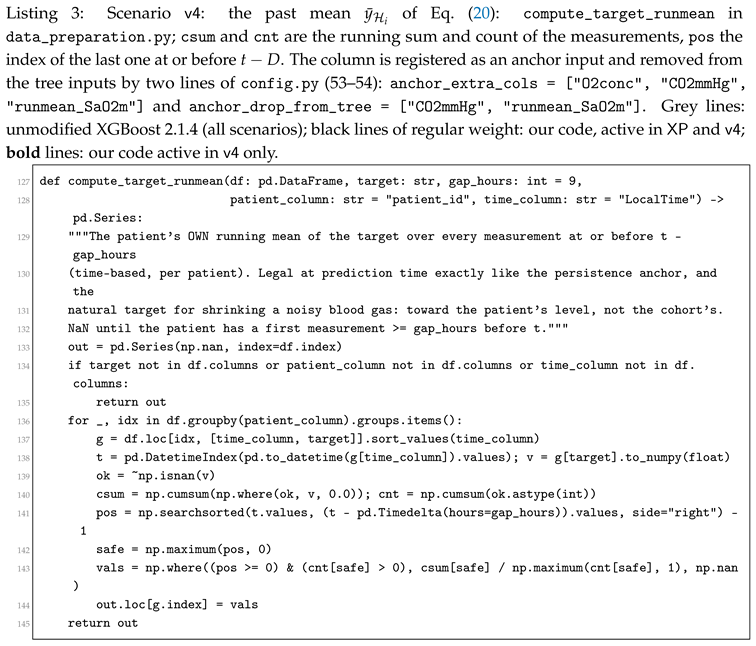
with in % and , dimensionless, and when is empty (the first D hours of a stay; utils_prediction.py). is the column runmean_SaO2m (data_preparation.py, compute_target_runmean). The three coefficients are the weighted least-squares solution on the training rows of the fold, with the weights of Eq. (2):
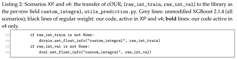
with defined by Eq. (20). In the implementation, the three anchor coefficients (, , , representing the intercept, persistence weight, and historical patient mean) are solved in Python and transferred via the base_margin field of the training and validation DMatrix objects. In the C++ core, this directly populates base_margin_ (), which acts as the initial reference score for each row in the tree recursion (Section 2.5) and the physiological anchor of the final ensemble prediction in Eq. (37).
Each cross-validation fold estimates these coefficients strictly using its training cohort and applies them out-of-fold to the held-out validation patients. The resulting fold-averaged coefficients are , , and (Section 3). Because , Eq. (20) represents, to within four percent, a weighted combination between the last measured blood gas () and the patient’s long-term historical baseline (). The theoretical rationale for assigning a weight strictly below unity to is regression attenuation [43,44]: framing the observed measurement as , where is the true underlying physiological state and represents independent measurement noise, the least-squares shrinkage slope on is
and carries the same level with less noise, so Eq. (21) moves weight from to , a shrinkage toward the patient’s own level [45].
2.5. The Boosted Tree Ensemble Shared by the Three Scenarios
The three scenarios share one boosted ensemble; what differs between them enters only through the initial prediction and the final prediction of Section 2.6. This subsection therefore describes the ensemble once. What is ours in this subsection. The ensemble is XGBoost 2.1.4 unchanged in all three scenarios; Section 2.5.1 states the four relations of its algorithm that our code touches and the three places where it does, without reproducing its derivations. Our contribution enters the ensemble at one place: the initial prediction from which the recursion of Eq. (31) starts, which is in X0 and XP, Eq. (19), and the patient-level anchor of Eq. (20) inv4. The final prediction of XP and v4, Eq. (37), is formed after the last tree and is not part of the recursion. Units: , , , the leaf scores and the gradients are in %; , the Hessians and their sums, and are dimensionless; is in %, the unit of the gradient sums; and the split gain are in ; the inputs are Z-scores. The library we patched and ran is XGBoost release 2.1.4; the excerpts of original XGBoost code in this subsection are copied, with their line numbers, from the release 2.1.4 files of the library we patched and ran, and are typeset in grey; the lines of our own additions are cited against the same sources (Section 2.4 and Section 2.6).
Boosting algorithms, such as the foundational AdaBoost [46], build ensemble models sequentially, where each new tree is specifically trained to correct the errors made by its predecessors [47]. XGBoost [47] improves upon traditional boosting by introducing a sparsity-aware split-finding algorithm for sparse data and a regularized learning objective to prevent overfitting, an approach since validated across many tabular clinical-prediction tasks [26,29]. Throughout this subsection the symbol ≡ denotes a definition. To keep the presentation uniform, every displayed equation is stated first and its newly introduced symbols are defined immediately afterwards in a where clause. The only exceptions are the few symbols that need a sentence of conceptual set-up (such as the routing and the leaf-score vector below): these are introduced in the prose that motivates their equation and are then not repeated. In no case is a symbol defined twice. The fixed global counts are written as n with a subscript naming what is counted: indexes the training samples, indexes the features, and indexes the boosting rounds (equivalently, the trees). The one count that varies from tree to tree, the number of leaves, is written , with leaf index ; it is a deliberately separate symbol from the tree count so the two can never be confused.
Input, target, and prediction.
Following the notation of Section 1, each sample i is one mechanically ventilated patient at one hour, described by the feature vector of Table 1 and Table 2, where is the number of features. The value of is a property of the scenario (Section 2.2, Table 1Table 2): in X0 and XP the trees receive columns, the six real-time signals at hour t, their 44 lagged copies, and five target-derived or static descriptors; in v4 they receive , five signals at t with two lags each and four descriptors. Grouping the columns by block, the input vector is
with in X0 and XP and in v4, where each component (for and ) is a single scalar feature and the superscript ⊤ denotes transposition, so is a column vector. The ground truth is the co-oximetry oxygen saturation in percent at hour t, a single scalar; to make every symbol concrete enough to check by hand, a small running example throughout this subsection uses five hypothetical hourly samples with target vector . These five are a didactic device for hand-calculation and do not redefine the dataset size, which in our actual run is in every scenario. Finally, the model’s prediction for sample i is a single scalar : its estimate of the true target , obtained by mapping the feature vector through the ensemble. Input , target , and prediction are the three quantities this paragraph names; the next paragraph constructs the map explicitly.
From the input to a prediction.
Having fixed what a single input from Eq. (23) is, we now build the function that turns it into the estimate . Chen and Guestrin [47] construct this function as a sum of regression trees, each tree adding one correction to the running estimate:
where is the raw boosted estimate of for sample i after the last round, denotes the full ensemble, is the per-row initial prediction of Section 2.4 (Eq. (19) in X0 and XP, Eq. (20) inv4), is the learning rate defined at Eq. (31), is the number of boosting rounds (capped at 2000 and chosen per fold by early stopping: on average trees in X0 and XP, in v4), and is the b-th regression tree, drawn from the tree space defined next. In X0 the final prediction is ; in XP and v4 it is the blend of Eq. (37).
What a single tree is.
A regression tree is a finite set of yes/no questions arranged as a binary tree, each question of the form "is feature m of the sample below the threshold ?", together with one number stored at every leaf. To evaluate the tree on a sample, one starts at the root, answers the question, moves to the left child on "yes" and to the right child on "no", and repeats until a leaf is reached; the tree’s output is the number stored at that leaf. Two objects therefore describe tree b completely. The first is the routing , which is the branch structure written as a function: is the index of the leaf that sample i reaches, and is defined for any feature vector, including ventilator readings never seen during training. The second is the leaf-score vector , one number per leaf. With the leaf reached, the output of the tree is
The same routing fixes which training samples share a leaf, and the objective derived below sums over those per-leaf groups; reappears in that role in Eq. (33).
The same routing fixes which training samples share a leaf, and the objective derived below sums over those per-leaf groups; reappears in that role in Eq. (33).
A concrete tree.
The purpose of this example is deliberately narrow: to exhibit the abstract pair of the previous paragraph on a tree small enough to check by hand. It draws on two results that are only derived later, how a leaf score is obtained in closed form (Eq. (35), Section 2.5.1) and how a split is chosen (Section 2.5.1), and states them here without proof so that the objects can be seen in action before the machinery that produces them is built. This illustrate first, derive later ordering is common in expository treatments; a reader may take the two results on trust until those sections. Concretely, take to be a depth-1 tree whose root splits on the inspired oxygen concentration at hour t, the first feature of the input, i.e. component of in Eq. (23), producing leaves:
The indices here are worth spelling out, because three different roles meet in this one equation. The value being tested, , is a feature of samplei, so it carries the sample index i and the feature index 1; it does not carry the round index b, since the input does not depend on which tree reads it. What does belong to tree b is the split rule, the choice to branch on component 1 and the threshold are parameters of this particular , which is exactly why the routing carries the subscript b. And the leaf index j does not appear on the input side at all: it is the output of the routing, , fed into Eq. (25) to read the score. Concretely, sample i with gives , so by (25) the tree outputs ; sample i with gives and output . Neither part of this tree is chosen by hand. XGBoost learns the leaf scores from the data through the closed form () below, and it learns the split structure, which feature each node tests, and at what threshold, through the greedy search of Section 2.5.1, which scans the candidate thresholds of every feature and keeps the one that maximizes the split gain (). The number is a didactic placeholder chosen to keep the arithmetic legible; it is not a fitted value from our run. The quantity it stands for is, at training time, the C++ variable split_pt that EnumerateSplit selects for the node (the third argument of best.Update in the listing of Section 2.5.1); once training finishes, that value is stored as the node’s split condition inside the fitted booster and can be read back from the Python model with model.get_booster().trees_to_dataframe() (the Split column) or get_dump(). All split thresholds and leaf weights are determined automatically by the tree-growing algorithm via gradient-based gain maximization during training, rather than by manually specified decision rules.
In the source code, a tree’s prediction and the objective registered as reg:squarederror are realized by the LinearSquareLoss struct; the routing and leaf storage are handled by the tree builder discussed in Section 2.5.1.1
How the trees are chosen: the training objective.
The ensemble (24) is only as good as the trees placed in it, so the trees are selected to minimize a training objective that balances how well the model fits the data against how complex it becomes. The objective is assembled from two ingredients. The first is the data-fit term: inserting the ensemble prediction of Eq. (24) into the squared-error loss (the factor is a convention that makes the gradient in Eq. (32) clean and does not change the minimizer) and summing over all samples gives the total prediction error . The second is a complexity penalty charged to each individual tree ,
which grows with that tree’s number of leaves (penalty rate , the gamma parameter, left at its default 0 in our runs) and with the squared magnitude of its leaf scores (rate , the strength reg_lambda ); the index runs over the leaves of that one tree, and is the score at leaf j of tree b (the j-th component of ). Now, because the ensemble of Eq. (24) is the sum of all trees, , the model’s total complexity is the sum of these per-tree penalties — one term for each of the trees — and this is precisely where the second summation below comes from. Adding the two ingredients yields the regularized objective of Chen and Guestrin [47]:
The two summations run over different index sets and therefore cannot be merged: the first is indexed by the sample , the second by the tree . Nor can the complexity be pulled outside its own sum, because genuinely differs from tree to tree — the leaf count and the scores both depend on b, while only the rates are shared — which is exactly why each carries the tree subscript b.
Making the loss cost-sensitive.
Finally, to make the predictions more sensitive to clinically critical low saturations, we insert the cost-sensitive sample weight of Eq. (2) into each loss term of the objective (29). This single substitution yields the weighted objective actually optimized in this study:
where from Eq. (2); the worked example uses the illustrative floor , exponent and stabiliser (the scenario values are in Table 8Table 9). For the five example targets these weights are all (the targets are large and similar), whereas a hypothetical desaturation to would raise that sample’s weight, up-weighting its contribution to the loss. Equation (30) is written here in the compact summary form used in the literature; the remainder of this subsection derives, step by step, how the trees that minimize it are actually built.
2.5.1. Training the Trees: Original XGBoost, and the Three Places Where Our Code Enters
The trees are trained by the gradient-boosting algorithm of XGBoost 2.1.4 exactly as released. We reproduce none of its derivations: the additive recursion is that of Friedman [48], and the second-order objective, the closed-form leaf score and the split gain are those of Chen and Guestrin [47], to which we refer for their proofs. We state only the four relations of that algorithm that our code touches, in the notation of this paper, so that each of our interventions can be located (Figure 2). Starting from the initial prediction , each round adds one tree scaled by the learning rate ; the tree of round b is fitted to the gradient and Hessian of the weighted squared loss at the previous prediction, summed over the training rows that its routing sends to leaf j; the leaf score and the gain of a split into children L and R follow in closed form with the penalties , and :
with the set of training rows in leaf j, in %, G and in %, H and dimensionless, and the gain and in ; a node is split while the gain is positive, both children keep a summed Hessian of at least min_child_weight and the depth is below max_depth, and otherwise it becomes a leaf with the score of Eq. (35). In the library, Eq. (32) is src/objective/regression_obj.cu, Eq. (35) is CalcWeight in src/tree/param.h, Eq. (36) is CalcGain applied inside EnumerateSplit in src/tree/hist/evaluate_splits.h, and the scaling by of Eq. (31). Our code enters this algorithm at three places, all of them before the first tree is grown, and modifies nothing inside it. First, the starting value of Eq. (31) is our anchor, the last available measurement in X0 and XP, Eq. (19), and the patient-level anchor of Eq. (20) inv4, passed as the base_margin of both matrices (utils_prediction.py) and copied by the library into the prediction buffer of every row before the first tree (Predictor::InitOutPredictions, src/predictor/predictor.cc); consequently every gradient of Eq. (32) is evaluated relative to the anchor, and every leaf score of Eq. (35) is a correction to it rather than to a constant. Second, the weights of Eq. (2), our relative-entropy criterion of Section 2.3, are the weight of the training matrix and multiply every gradient and Hessian (regression_obj.cu). Third, the hyperparameters , , , , max_depth, min_child_weight, the two subsampling ratios and the early-stopping patience are set per scenario (Table 8 and Table 9). The library’s evaluation of the validation rows after each round (src/learner.cc) sees the unblended and chooses the number of trees by early stopping (Section 2.8.1): on average trees per fold with leaves each in X0 and XP, and trees with leaves in v4 (Table 10). After the last tree, the final prediction of Section 2.6 is formed; it is ours and is not part of the training. The reason the anchor changes what the trees learn is visible in Eq. (32): with the raw persistence anchor, the first gradients are the errors of a noisy nine-hour-old value, and the trees spend their capacity on pulling it toward the patient’s level, which appears as a negative variance share of the trees in Section 3.3; with the patient-level anchor that work is done in closed form before boosting, and a far smaller ensemble suffices.
2.6. The Final Prediction
The trees give the raw boosted estimate of Eq. (24). After the last tree, our C++ function ApplyAnchorBlend forms the final prediction (%) of every row, training and validation rows alike:
where the dimensionless (custom_b) pulls the prediction toward its initial value and (% kg h−1 a.u.−1; custom_b1) weighs the cumulative oxygen uptake rate of Eq. (16): in X0, in XP (config.py) and in v4 (locked configuration file). Substituting Eq. (24), which gives , together with Eqs. (20) and (16), into Eq. (37) writes the prediction of v4 in its original quantities:
In X0 and XP the first term is , Eq. (19). Table 6 gives, for every term of Eq. (38), the Python variable that holds it, how it reaches src/learner.cc, where it is read and when it is used.
Table 6.
The terms of Eq. (38) in the code. File utils_prediction.py unless stated; C++ lines in src/learner.cc.
Table 6.
The terms of Eq. (38) in the code. File utils_prediction.py unless stated; C++ lines in src/learner.cc.
| Term | Python | In C++ | Used in |
|---|---|---|---|
| , , | coef[0..2]; | not present; they act through | through |
| , | columns SaO2m_lag_9h, runmean_SaO2m | not present | through |
| raw_base_train, raw_base_val; base_margin | base_margin_: start of the prediction buffer before the first tree; anchor | training rounds, early stopping, prediction | |
| the trees, trained by xgb.train | PredictRaw (training), (early stopping),(prediction) | training rounds, early stopping, prediction | |
| raw_int_train, raw_int_val;set_float_info("custom_integral",...), | our field custom_integral_ (declared in include/xgboost/data.h; filled by MetaInfo::SetInfo, src/data/data.cc; C API src/c_api/c_api.cc) | prediction | |
| , | params["custom_b"], params["custom_b1"]; xgb.train(params=params, ...) | tparam_.custom_b, tparam_.custom_b1 | prediction |
The predicted saturation is formed in Predict: PredictRaw evaluates the trees from and gives , and ApplyAnchorBlend overwrites it in place with . Python receives from bst.predict(dval) for the validation rows, which are the reported out-of-fold predictions, and from bst.predict(dtrain) for the training rows. and therefore act on the predictions of training and validation rows alike, but not on the training loss or the early-stopping criterion: UpdateOneIter and EvalOneIter never call ApplyAnchorBlend. For and , Eq. (37) is the convex combination , hence by the triangle inequality
which is why custom_b is declared on and why Eq. (37) is applied once, after the last tree: applied once per boosting round it would compound to and Eq. (39) would not hold.
2.7. Anatomy of a Prediction: How Much Is Physics and How Much Is Trees
Eq. (38) splits every final prediction exactly into three parts, written next to every out-of-fold row by the pipeline (anchorpart, treepart, integralpart; utilsprediction.py):
all in %. For each part the variance share and the work share are
with for A and for B and C, and the error credit of the anchor is
with MAPE as in Eq. (43). By bilinearity of the covariance, substituting Eq. (40) into Eq. (41) gives , so the three variance shares sum to 100%; a negative share means that the part moves against the prediction. The work share says how far each part moves the prediction away from the last available measurement, and the error credit which fraction of the improvement over it the anchor earns before any tree is grown.
2.8. Training and Evaluation Strategy
To avoid overly optimistic performance estimates caused by temporal correlation within the same patient trajectory, we implemented a 5-fold Grouped Cross-Validation strategy. In this configuration, data is partitioned such that all samples of a patient are kept together within a single fold. This ensures that no data from the same patient used during the training phase is ever present in the test set, effectively preventing data leakage. The patient-level fold assignment is shuffled with a fixed random seed (random_state ), which also seeds the XGBoost estimator, so that the entire pipeline is reproducible; every scenario uses the same folds.
Target-history leakage and the strict gap.
Because two of the inputs are the target’s own past values ( at and ), the validity of the reported error depends critically on which target lags are admitted as features. The blood-gas measurement that defines is itself delayed by roughly nine hours, so at deployment the freshest genuinely available value of the target is its 9-hour lag; any value of from the intervening eight hours (), and any feature derived from future samples, would simply not exist at prediction time. If such a near-past or future value of the target were allowed into the feature set, the model would in effect be shown a lightly time-shifted copy of the answer: the reported MAPE would collapse to an optimistically small figure, and the “virtual sensor” would be quietly reading the very signal it is meant to reconstruct rather than inferring it from ventilator and gas measurements. The pipeline constructs only target lags of nine hours or more. It does not, however, discard the rows that lack a nine-hour lag: in the first nine hours of a stay it fills the lag with the patient’s first measurement (fallback_to_first=True), and SaO2m_first and the patient mean carry the same value, so these 287 rows () see a value fresher than , and 33 of them the current target itself. By the rule above these rows are invalid; all results of Section 3 are computed without them, so that the estimator at hour t sees the real-time gas and ventilator channels plus target history no fresher than . It is important to stress that the patient-grouped cross-validation above does not on its own guard against this particular failure: grouping by patient eliminates between-patient leakage, but a near-past or future copy of a patient’s own target leaks within that patient’s trajectory, which grouped folds cannot detect. The headline accuracy must therefore be read as conditional on the strict-gap construction; relaxing it, admitting sub-gap target lags, or back-filling missing values from later rows, would lower the apparent error without any gain in genuine predictive power, and any such configuration should be treated as invalid for the nine-hour-ahead claim.
The primary evaluation metric utilized in this study is the Mean Absolute Percentage Error (MAPE), as it provides a relative measure of error that is clinically informative across varying oxygenation levels. The MAPE is defined as:
Equation (43) is the pooled, row-weighted MAPE. Three patients (18, 3 and 21) hold about 85% of the squared error of every scenario, and five patients have hours with two readings, so the pooled MAPE mostly reports those patients. We therefore report, for every scenario, the per-patient MAPE
and three summaries of it over the patients: the macro MAPE, its mean; the trimmed MAPE, its mean without the three worst patients; and its median. The macro MAPE is the objective that the pruning and the tuning of v4 used. Tracking within a patient is measured by
which is positive only when the model beats the patient’s own mean; its median over patients is reported together with the same quantity computed for persistence, the floor a virtual sensor must beat, and with the number of patients in which the model beats persistence. The pooled Pearson correlation r between and y is reported as in our earlier work, with the caveat that it is lifted by between-patient level differences.
2.8.1. Training Rows and Validation Rows
In each fold the rows of 24 or 25 patients are training rows and the rows of the other 6 or 7 patients are validation rows; the reported predictions are those of the validation rows. Table 7 lists every place where the two are treated differently.
Two consequences follow. The training loss and the early-stopping criterion never see and : the blend of Eq. (37) exists only at prediction time. And the validation rows choose through early stopping, so they are not entirely unseen during training; the folds are identical in every scenario, so the comparison between scenarios is not affected.
Hyperparameters of each scenario.
X0 and XP use the configured operating point of our pipeline (config.py; Table 8); X0 differs from XP only in . The hyperparameters of v4 (Table 9) were selected by a tree-structured Parzen estimator search (Optuna [49]) on the same patient-grouped folds for the 19-input tree with an earlier anchor, and were kept unchanged when the anchor of Eq. (20) was introduced; v4 itself was not re-tuned. Its lag lists (Table 1) were reduced from those of X0 and XP by lag-group ablation on the same folds; the column O2diffxPower is hidden from its trees because it feeds Eq. (16), and Svoris was hidden by a knockout test on the same folds. The configuration is fixed in the locked configuration file (Section 2.8.1.2).
Table 7.
What differs between training and validation rows within a fold. File and line refer to the delivered sources.
Table 7.
What differs between training and validation rows within a fold. File and line refer to the delivered sources.
| Step | Training rows | Validation rows | Code |
|---|---|---|---|
| standardisation of the tree inputs | scaler fitted and applied | training scaler applied | data_preparation.py |
| , , | from the row’s own past | the same formula | data_preparation.py |
| anchor coefficients, Eq. (21) | fitted | applied, not fitted | utils_prediction.py |
| sample weights | in the loss | none | utils_prediction.py |
| trees | fitted to the gradients | not used for fitting | utils_prediction.py |
| after each round | enters the gradients | enters the early-stopping RMSE, unweighted and without the blend | learner.cc |
| number of trees | — | decided by early stopping | utils_prediction.py |
| final prediction, Eq. (37) | computed | computed; reported out of fold | learner.cc |
Table 8.
Hyperparameters of X0 and XP (config.py and the TrainConfig block). X0 sets ; everything else is identical.
Table 8.
Hyperparameters of X0 and XP (config.py and the TrainConfig block). X0 sets ; everything else is identical.
| Parameter (name in the code) | Value | Role |
|---|---|---|
| learning_rate () | step applied to each tree’s correction, Eq. (31) | |
| n_estimators ( cap) | 2000 | ceiling on the tree count; early stopping selects on average |
| early_stopping_rounds | 100 | rounds without validation improvement before halting |
| max_depth | 4 | maximum tree depth |
| min_child_weight | minimum summed Hessian per leaf (the IsValid guard) | |
| reg_lambda () | penalty on leaf scores, Eq. (35) | |
| reg_alpha () | penalty on leaf scores | |
| gamma () | 0 | minimum gain to accept a split |
| subsample | fraction of rows per tree | |
| colsample_bytree | fraction of columns per tree | |
| tree_method | hist | histogram split finding |
| custom_b () | 0 (X0) / (XP) | anchor blend, Eq. (37) |
| custom_b1 () | 0 (X0) / (XP) | integral weight, Eq. (37) |
| custom_power (), custom_kp () | , | cost weights, Eq. (2); inert on this target range (Section 3.5) |
| random_state | 42 | fold shuffle and model seed |
Table 9.
Hyperparameters of v4 (locked configuration file locked_model_v4.json, keys xgb_params, train and runtime), selected by the search described in the text.
Table 9.
Hyperparameters of v4 (locked configuration file locked_model_v4.json, keys xgb_params, train and runtime), selected by the search described in the text.
| Parameter (name in the code) | Value | Role |
|---|---|---|
| learning_rate () | step applied to each tree’s correction | |
| n_estimators ( cap) | 2000 | ceiling; early stopping selects trees on average |
| early_stopping_rounds | 50 | patience |
| max_depth | 3 | maximum tree depth |
| min_child_weight | minimum summed Hessian per leaf | |
| reg_lambda () | penalty on leaf scores | |
| reg_alpha () | penalty on leaf scores | |
| subsample, colsample_bytree | , | row and column fractions per tree |
| custom_b () | anchor blend, Eq. (37) | |
| custom_b1 () | integral weight, Eq. (37) | |
| mass_balance=calib_pt | — | the anchor of Eq. (20), fitted per fold |
| tree_exclude | O2diffxPower, Svoris | columns hidden from the trees |
| custom_power (), custom_kp () | , | cost weights; inert (Section 3.5) |
Reproducibility.
Each scenario is fully specified by one configuration: X0 and XP by config.py with or with their configured values, and v4 by a locked JSON file that records its lag lists, the columns hidden from the trees, the anchor mode and every hyperparameter; XGB_LOCKED=<file> python train.py re-trains it and reproduces the metrics of Section 3 exactly (same folds, same seed). The three scenarios were evaluated in one run on identical folds, and the out-of-fold prediction of every row was stored together with its three parts of Eq. (40).
3. Results
All results are out-of-fold predictions under the patient-grouped five-fold cross-validation of Section 2.8, with identical folds for the three scenarios. Following the rule of Section 2.8, they are scored on the 3730 rows of 30 patients whose inputs contain no value younger than nine hours (Section 3.7); the values on all 4017 rows are listed alongside in Table 14. A patient counts as beating persistence when its , Eq. (45), exceeds that of .
3.1. Accuracy and Size of the Three Scenarios
Table 10 reports accuracy and size. The C++ terms of XP lower the macro MAPE by 0.032 percentage points: a paired patient bootstrap of XP − X0 (2000 resamples of the 30 patients) gives with 95% interval , while the intervals of the pooled (, ), trimmed (, ) and median per-patient MAPE (, ) include zero; 17 of the 30 patients improve. The effect of XP is therefore small and resolved only for the mean per-patient error. The patient-level anchor of v4 lowers, relative to XP, the pooled MAPE by 0.163 (), the macro MAPE by 0.172 () and the trimmed MAPE by 0.142 (), while the change of the median, (), is not resolved; 22 of the 30 patients improve. v4 raises the pooled correlation from 0.754 to 0.793 and the median within-patient from to , beats persistence in 29 of the 30 patients, and does so with 19 inputs instead of 55, 83 trees instead of 792 and 450 leaves per fold instead of 9527. Keeping only the last of two readings in the same hour (3427 strict rows) changes the pooled MAPE to 3.919% (X0), 3.898% (XP) and 3.741% (v4) and leaves the ranking unchanged.
Table 10.
Out-of-fold accuracy and size on the 3730 rows of 30 patients whose inputs contain no value younger than nine hours; identical patient-grouped folds. Trees and leaves are per-fold means. The persistence column scores itself, with no model.
Table 10.
Out-of-fold accuracy and size on the 3730 rows of 30 patients whose inputs contain no value younger than nine hours; identical patient-grouped folds. Trees and leaves are per-fold means. The persistence column scores itself, with no model.
| Quantity | Persistence | X0 | XP | v4 |
|---|---|---|---|---|
| tree inputs | — | 55 | 55 | 19 |
| trees per fold | — | 792.4 | 792.4 | 83.2 |
| leaves per fold | — | 9527.4 | 9527.4 | 450.2 |
| pooled MAPE (%) | 4.308 | 3.900 | 3.890 | 3.727 |
| macro MAPE (%) | 3.499 | 3.321 | 3.289 | 3.117 |
| trimmed MAPE (%) | 2.038 | 1.878 | 1.850 | 1.709 |
| median per-patient MAPE (%) | 1.982 | 1.875 | 1.815 | 1.742 |
| pooled Pearson r | 0.728 | 0.754 | 0.754 | 0.793 |
| median | ||||
| patients beating persistence (of 30) | — | 27 | 27 | 29 |
3.2. The Anchor Coefficients of v4
Table 11 lists the coefficients of Eq. (20) fitted on each training fold. and keep their sign in every fold, and their sum is on average, so the anchor is, to four per cent, a weighted average that gives the nine-hour-old measurement of the weight and the patient’s own history ; the intercept is small and changes sign across folds. The anchor alone, before any tree, has a pooled MAPE of against for the persistence value it recalibrates.
Table 11.
Coefficients of the v4 anchor, Eq. (20), per training fold (locked configuration file, key anchor_coefficients_per_fold).
Table 11.
Coefficients of the v4 anchor, Eq. (20), per training fold (locked configuration file, key anchor_coefficients_per_fold).
| Fold | (last measurement) | (patient history) | ||
|---|---|---|---|---|
| 1 | ||||
| 2 | ||||
| 3 | ||||
| 4 | ||||
| 5 | ||||
| mean |
3.3. How Much of Each Prediction Is Physics
Table 12 applies the shares of Section 2.7 to the strict rows. In X0 and XP the anchor is the raw persistence value and the trees’ variance share is negative (, ): the trees pull the noisy nine-hour-old value toward the patient’s level, which is the shrinkage of Eq. (22) done split by split with 792 trees. In v4 the anchor of Eq. (20) does this in closed form: alone it lowers the pooled MAPE from 4.308% (persistence) to 3.836%, which is 81% of the improvement of the full model (3.727%), it does 71% of the work, and the 83-tree ensemble corrects single rows while adding 1% of the variance. On the median patient the trees add nothing: the anchor alone has a median per-patient MAPE of 1.703%, the full v4 model 1.742%. The identity holds to on every row.
Table 12.
Shares of Eqs. (41)–(42) in per cent on the strict rows. The variance shares of the three parts sum to 100.
| Share (%) | X0 | XP | v4 |
|---|---|---|---|
| variance share of the anchor A | 113.65 | 113.99 | 99.94 |
| variance share of the trees B | 1.02 | ||
| variance share of the cumulative OUR term C | 0.00 | ||
| work share of the anchor A | 0.00 | 0.00 | 71.33 |
| work share of the trees B | 100.00 | 84.76 | 20.44 |
| work share of the cumulative OUR term C | 0.00 | 15.24 | 8.23 |
| error credit of the anchor | 0.00 | 0.00 | 81.27 |
| pooled MAPE of the anchor alone (%) | 4.308 | 4.308 | 3.836 |
3.4. Ablation of the Two C++ Coefficients in v4
Table 13 evaluates the trained v4 model with , or both set to zero in Eq. (37). The two coefficients act only on the predictions (Section 2.6), so the trees are the same in every row of the table, and each row measures what a coefficient contributes to the predictions of the validation rows. The predictions with a coefficient set to zero are not stored row by row, so the table is on all 4017 rows. Setting raises the pooled MAPE by 0.032 percentage points, the trimmed by 0.027 and the median by 0.061; setting raises the pooled, macro and trimmed MAPE by about 0.004 and lowers the median by 0.025. Both coefficients are kept by our rule that a physics coefficient is set to zero only when doing so changes the median per-patient MAPE by at most 0.001 and the macro by at most 0.005.
Table 13.
Change of each metric when a coefficient of Eq. (37) is set to zero in the trained v4 model; all 4017 rows, percentage points.
Table 13.
Change of each metric when a coefficient of Eq. (37) is set to zero in the trained v4 model; all 4017 rows, percentage points.
| Set to zero | pooled | macro | trimmed | median |
|---|---|---|---|---|
3.5. The Cost Weights Are Inert
The recorded target ranges from 20 to 111 % (Section 2.1). Over all 4017 rows, the largest relative deviation of from in Eq. (2) is in X0 and XP (, ) and in v4 (, ), so the weights are constant to that precision and the weighted least squares of Eq. (21) and the weighted objective of the trees are unweighted in effect: the tuned values sit at the variance end of the trade-off of Eq. (5). The squared-relative-error end would matter only if were comparable with , which for y between 50 and 100 % requires of order at , below the range the tuning explored; exploring it is left for future work.
3.6. The Age of the Anchor and the Persistence Baseline
The persistence value is the most recent measurement at or before h, Eq. (17). Of the 4017 rows, have an anchor exactly nine hours old; have an older one (median age h, 90th percentile h, maximum 81 h) because no measurement fell in the preceding hour; and lie in the first nine hours of a stay and use the patient’s first measurement, whose age is below nine hours and is zero in 33 rows (): the first row of each patient and, for patients 2 and 3, a second reading in that same hour. Because the target is integer-valued, the nine-hour-old value equals the target exactly in of the rows; in the rows that have a measurement at least nine hours old this is quantisation of the label, not leakage, and it sets the floor that Table 10 reports for persistence.
3.7. Strict Nine-Hour Check
The target-derived inputs use values younger than nine hours in one situation: when a patient has no measurement at or before , that is, in the first D hours of a stay. There and SaO2m_lag_10h fall back to the patient’s first measurement (data_preparation.py, called with fallback_to_first=True), is filled with the same value (utils_prediction.py), and the tree input SaO2m_first is that first measurement too (data_preparation.py). This concerns 287 of the 4017 rows () in every scenario, and in 33 of them the value used is the current target itself; one patient has no row outside this window, so the strict rows cover 30 patients. No value from a later hour is used anywhere: the lags are taken with a backward merge, the patient mean stops at , and SaO2m_first is the earliest reading. Because the validation patients of a fold never appear among its training patients, these inputs in training rows carry no information about the validation rows; removing the 287 rows at scoring therefore leaves out-of-fold predictions whose inputs contain no value younger than nine hours. Table 14 compares the two evaluations.
Table 14.
Out-of-fold metrics on all 4017 rows (31 patients) and on the 3730 strict rows (30 patients).
Table 14.
Out-of-fold metrics on all 4017 rows (31 patients) and on the 3730 strict rows (30 patients).
| X0 | XP | v4 | ||||
|---|---|---|---|---|---|---|
| Metric | all | strict | all | strict | all | strict |
| pooled MAPE (%) | 3.791 | 3.900 | 3.766 | 3.890 | 3.603 | 3.727 |
| macro MAPE (%) | 3.272 | 3.321 | 3.209 | 3.289 | 3.029 | 3.117 |
| trimmed MAPE (%) | 1.962 | 1.878 | 1.906 | 1.850 | 1.758 | 1.709 |
| median per-patient MAPE (%) | 1.936 | 1.875 | 1.850 | 1.815 | 1.737 | 1.742 |
| pooled Pearson r | 0.763 | 0.754 | 0.764 | 0.754 | 0.801 | 0.793 |
The ranking of the three scenarios is the same in both evaluations. A deployable sensor under the strict rule starts nine hours after a patient’s first measurement; rows before that point would need a population prior as the anchor, which is not part of this study.
4. Discussion
Three findings carry the paper, all measured on the rows whose inputs contain no value younger than nine hours. First, the physics pays through the anchor. The patient-level recalibration of v4 is a two-coefficient linear term, yet on its own it earns 81% of the improvement over persistence, and with it the pooled, macro and trimmed errors fall by 0.14 to 0.17 percentage points relative to XP, with bootstrap intervals that exclude zero, while the tree ensemble shrinks to 19 inputs and 450 leaves. Second, the anatomy of Table 12 explains why: with a raw persistence anchor the trees spend a negative variance share on shrinking a noisy measurement toward the patient’s level, a task that Eq. (22) performs in closed form once the patient’s own history is available; freed from it, a much smaller ensemble corrects single rows. Third, the direct contribution of the gas signals through the physics terms is small: the cumulative oxygen uptake rate and the blend of XP lower the mean per-patient error by 0.032 percentage points, an effect whose interval only just excludes zero and which the pooled, trimmed and median summaries do not resolve.
What the sensor does and does not do is now explicit. It reproduces each patient’s level and beats the last blood gas in 29 of 30 patients; it does not resolve hourly changes for typical patients, whose hourly standard deviation of about 1.9 percentage points is at the label’s integer quantisation, and the median within-patient stays negative in all scenarios. The median per-patient error is not resolved by either step, and on the median patient the anchor of v4 alone is as accurate as the full model.
The claims are bounded by the design. The cohort is small (30 patients on the strict rows), and three patients hold most of the squared error, which is why the macro, trimmed and median per-patient errors are reported next to the pooled one and every difference is tested with a paired patient bootstrap. The validation rows decide the number of trees through early stopping, which is common to all scenarios and therefore does not favour one of them. The training rows still include the first nine hours of the training patients’ stays; this carries no information about the validation patients, but a pipeline that drops these rows from training as well would be the natural next version.
Within the scope of this Special Issue, the model is a multivariate time-series application with an explicit account of what each component contributes, and its loss is the relative-entropy criterion of our earlier estimators; a natural next step is to add information-theoretic descriptors of the ventilator channels (permutation or sample entropy over the same lag windows) as tree inputs and to test whether they carry the within-patient dynamics that the present inputs do not.
5. Conclusions
A virtual sensor for arterial oxygen saturation across a nine-hour blood-gas gap was built as three nested scenarios of one code base and evaluated on identical folds on the rows whose inputs contain no saturation value younger than nine hours. Adding to XGBoost 2.1.4 a blend toward the anchor and the cumulative oxygen uptake rate over the gap, derived from an oxygen balance of the arterial blood (XP), gives a small improvement of the mean per-patient error. Replacing the raw nine-hour-old measurement by a patient-level calibrated anchor (v4) lowers the pooled, macro and trimmed errors with bootstrap intervals that exclude zero, beats the last blood gas in 29 of 30 patients, and reduces the ensemble to 19 inputs and 450 leaves; the anchor alone earns 81% of the gain over persistence. Every equation is matched to the line of C++ or Python that implements it, and each scenario is reproducible from one configuration file.
Author Contributions
Conceptualization, R.U.; methodology, R.U., S.R. and V.Ga.; software, R.U. and N.P.; validation, R.U., N.P. and V.Ga.; formal analysis, R.U. and N.P.; investigation, R.U. and N.P.; resources, R.U and V.Ga.; data curation, R.U. and T.K.; writing—original draft preparation, R.U. and N.P.; writing—review and editing, R.U., N.P. and V.Ga.; visualization, R.U. and N.P.; supervision, R.U., L.J. and V.Ga.; project administration, R.U., V.Ga. and V.Gu.; funding acquisition, V.Ga All authors have read and agreed to the published version of the manuscript.
Funding
This research is funded by the Research Council of Lithuania (Grant No. S-ITP-25-1).
Institutional Review Board Statement
The medical study for collecting engineering data is carried out under the permit BE-2-92 granted by the Kaunas Regional Biomedical Research Ethics Committee.
Informed Consent Statement
Informed consent was obtained from the legal representatives of all patients involved in the study.
Data Availability Statement
The changes to XGBoost 2.1.4 (src/learner.cc, and the field custom_integral in include/xgboost/data.h, src/data/data.cc and src/c_api/c_api.cc) are available from the corresponding author on reasonable request. The key functions of the Python pipeline are given in the listings of this paper. The patient data are not publicly available for privacy reasons.
Acknowledgments
The authors thank the Lithuanian University of Health Sciences Hospital Kauno Klinikos (Kaunas, Lithuania) for the collaboration in the pending clinical trials. During the preparation of this manuscript, the authors used Open AI models for the purpose of language editing and assistance in drafting text. The authors reviewed and edited the content as needed and take full responsibility for the content of the publication.
Conflicts of Interest
The authors declare no conflicts of interest.
Abbreviations
The following abbreviations are used in this manuscript:
| arterial oxygen saturation measured by co-oximetry | |
| MAPE | mean absolute percentage error |
| OOF | out of fold |
| PEEP | positive end-expiratory pressure |
| OUR | oxygen uptake rate |
| TPE | tree-structured Parzen estimator |
References
- Dall’Ora, C.; Saville, C.; Rubbo, B.; Turner, L.; Jones, J.; Griffiths, P. Nurse staffing levels and patient outcomes: A systematic review of longitudinal studies. Int. J. Nurs. Stud. 2022, 134, 104311. [Google Scholar] [CrossRef]
- Bertoni, M.; Spadaro, S.; Goligher, E.C. Monitoring Patient Respiratory Effort During Mechanical Ventilation: Lung and Diaphragm-Protective Ventilation. Crit. Care 2020, 24, 106. [Google Scholar] [CrossRef]
- Nguyen, L.S.; Squara, P. Non-invasive monitoring of cardiac output in critical care medicine. Front. Med. 2017, 4. [Google Scholar] [CrossRef]
- Athaya, T.; Choi, S. A Review of Noninvasive Methodologies to Estimate the Blood Pressure Waveform. Sensors 2022, 22. [Google Scholar] [CrossRef]
- Dong, J.; Xu-Wilson, M.; Conroy, B.R.; Khemani, R.G.; Newth, C.J.L. Continuous noninvasive blood gas estimation in critically ill pediatric patients with respiratory failure. Sci. Rep. 2022, 12. [Google Scholar] [CrossRef]
- Krzych, L.; Wojnarowicz, O.; Ignacy, P.; Dorniak, J. Be cautious during the interpretation of arterial blood gas analysis performed outside the intensive care unit. Acta Biochim. Pol. 2020, 67, 353–358. [Google Scholar] [CrossRef]
- Patharkar, A.; Cai, F.; Al-Hindawi, F.; Wu, T. Predictive modeling of biomedical temporal data in healthcare applications: review and future directions. Front. Physiol. 2024, 15. [Google Scholar] [CrossRef]
- Lee, J.M.; Hauskrecht, M. Modeling multivariate clinical event time-series with recurrent temporal mechanisms. Artif. Intell. Med. 2021, 112. [Google Scholar] [CrossRef]
- Dauvin, A.; Donado, C.; Bachtiger, P.; Huang, K.C.; Sauer, C.M.; Ramazzotti, D.; Bonvini, M.; Celi, L.A.; Douglas, M.J. Machine learning can accurately predict pre-admission baseline hemoglobin and creatinine in intensive care patients. npj Digit. Med. 2019, 2. [Google Scholar] [CrossRef]
- Kipnis, E.; Ramsingh, D.; Bhargava, M.; Dincer, E.; Cannesson, M.; Broccard, A.; Vallet, B.; Bendjelid, K.; Thibault, R. Monitoring in the Intensive Care. Crit. Care Res. Pract. 2012, 2012, 473507. [Google Scholar] [CrossRef]
- Qiu, X.; Tan, X.; Wang, C.; Chen, S.; Du, B.; Huang, J. A long short-term memory relation network for real-time prediction of patient-specific ventilator parameters. Math. Biosci. Eng. 2023, 20, 14756–14776. [Google Scholar] [CrossRef]
- The Acute Respiratory Distress Syndrome Network.; Brower, R.G.; Matthay, M.A.; Morris, A.; Schoenfeld, D.; Thompson, B.T.; Wheeler, A. Ventilation with Lower Tidal Volumes as Compared with Traditional Tidal Volumes for Acute Lung Injury and the Acute Respiratory Distress Syndrome. N. Engl. J. Med. 2000, 342, 1301–1308. [Google Scholar] [CrossRef]
- Brower, R.G.; Lanken, P.N.; MacIntyre, N.; Matthay, M.A.; Morris, A.; Ancukiewicz, M.; Schoenfeld, D.; Thompson, B.T. National Heart, Lung, and Blood Institute ARDS Clinical Trials Network. Higher versus Lower Positive End-Expiratory Pressures in Patients with the Acute Respiratory Distress Syndrome. N. Engl. J. Med. 2004, 351, 327–336. [Google Scholar] [CrossRef]
- Zhang, L.; Ren, G.; Li, S.; Du, J.; Xu, D.; Li, Y. A novel soft sensor approach for industrial quality prediction based TCN with spatial and temporal attention. Chemom. Intell. Lab. Syst. 2025, 257. [Google Scholar] [CrossRef]
- Wang, C.; He, T.; Zhou, H.; Zhang, Z.; Lee, C. Artificial intelligence enhanced sensors - enabling technologies to next-generation healthcare and biomedical platform. Bioelectron. Med. 2023, 9, 17. [Google Scholar] [CrossRef]
- Li, J.; Ma, J.; Omisore, O.M.; Liu, Y.; Tang, H.; Ao, P.; Yan, Y.; Wang, L.; Nie, Z. Noninvasive Blood Glucose Monitoring Using Spatiotemporal ECG and PPG Feature Fusion and Weight-Based Choquet Integral Multimodel Approach. IEEE Trans. Neural Netw. Learn. Syst. 2024, 35, 14491–14505. [Google Scholar] [CrossRef]
- Quamer, W.; Tseng, M.R.; Vyas, K.; Dave, D.; Villegas, C.; McKay, S.; DeSalvo, D.J.; Erranguntla, M.; Cote, G.; Gutierrez-Osuna, R. A multimodal physiological dataset for non-invasive blood glucose estimation. Sci. Data 2025, 12. [Google Scholar] [CrossRef]
- Tsou, P.H.; Lin, Z.L.; Pan, Y.C.; Yang, H.C.; Chang, C.J.; Liang, S.K.; Wen, Y.F.; Chang, C.H.; Chang, L.Y.; Yu, K.L.; et al. Exploring volatile organic compounds in breath for high-accuracy prediction of lung cancer. Cancers 2021, 13, 1–14. [Google Scholar] [CrossRef]
- Choo, Y.J.; Lee, G.W.; Moon, J.S.; Chang, M.C. Application of non-contact sensors for health monitoring in hospitals: a narrative review. Front. Med. 2024, 11. [Google Scholar] [CrossRef]
- Nan, X.; Wang, X.; Kang, T.; Zhang, J.; Dong, L.; Dong, J.; Xia, P.; Wei, D. Review of Flexible Wearable Sensor Devices for Biomedical Application. Micromachines 2022, 13, 1395. [Google Scholar] [CrossRef]
- Moraes, F.M.D.; Silva, G.S. Noninvasive intracranial pressure monitoring methods: A critical review. Arq. De Neuro-Psiquiatr. 2021, 79, 437–446. [Google Scholar] [CrossRef]
- Wolber, J.; Schuppert, A.; Mücke, M.; Sellin, J. Predicting disease outcomes from remote monitoring using machine learning: a systematic review. BMC Med. Inform. Decis. Mak. 2026, 26. [Google Scholar] [CrossRef]
- Skarysz, A.; Salman, D.; Eddleston, M.; Sykora, M.; Hunsicker, E.; Nailon, W.H.; Darnley, K.; McLaren, D.B.; Thomas, C.L.P.; Soltoggio, A. Fast and automated biomarker detection in breath samples with machine learning. PLoS ONE 2022, 17. [Google Scholar] [CrossRef]
- Lee, A.R.; Lee, J.H.; Yoo, S.; Lee, H.Y.; Kim, H.H. Real-Time Estimation of Arterial Partial Pressure of Carbon Dioxide in Patients Undergoing General Anesthesia: Predictive Modeling Study. JMIR Med. Inform. 2025, 13. [Google Scholar] [CrossRef]
- Che, Z.; Purushotham, S.; Cho, K.; Sontag, D.; Liu, Y. Recurrent Neural Networks for Multivariate Time Series with Missing Values. Sci. Rep. 2018, 8, 6085. [Google Scholar] [CrossRef]
- Woo, J.W.; Stapleton, O.; Luo, J.; Chuang, C.C.; Su, Y.; Sankararaman, S.; Mukherjee, E.; Sivakumar, N.; Calligy, K.; Duffy, S.; et al. AI-Driven SaO2 prediction from pulse oximetry and electronic health records. BioData Min. 2025, 18. [Google Scholar] [CrossRef]
- Cabanas, A.M.; Martín-Escudero, P.; Pagán, J.; Mery, D. Technical and regulatory challenges in artificial intelligence-based pulse oximetry: a proposed development pipeline. Br. J. Anaesth. 2025, 134, 1295–1299. [Google Scholar] [CrossRef]
- Ghazal, S.; Sauthier, M.; Brossier, D.; Bouachir, W.; Jouvet, P.A.; Noumeir, R. Using machine learning models to predict oxygen saturation following ventilator support adjustment in critically ill children: A single center pilot study. PLoS ONE 2019, 14. [Google Scholar] [CrossRef]
- Hüser, M.; Lyu, X.; Faltys, M.; Pace, A.; Berger, D.; Hoche, M.; Hyland, S.L.; Yèche, H.; Burger, M.; Merz, T.M.; et al. RMS: a ML-based system for ICU respiratory monitoring and resource planning. npj Digit. Med. 2025, 8. [Google Scholar] [CrossRef]
- Si, T.; Song, Y.; Sun, P.; Xiao, J.; Zou, R.; Chen, Z. Non-contact SpO2 monitoring via multi-channel pulse signals from facial videos using machine learning. Mach. Vis. Appl. 2025, 36. [Google Scholar] [CrossRef]
- Urniezius, R.; Survyla, A.; Paulauskas, D.; Bumelis, V.A.; Galvanauskas, V. Generic estimator of biomass concentration for Escherichia coli and Saccharomyces cerevisiae fed-batch cultures based on cumulative oxygen consumption rate. Microb. Cell Fact. 2019, 18, 190. [Google Scholar] [CrossRef]
- Urniezius, R.; Survyla, A. Identification of Functional Bioprocess Model for Recombinant E. Coli Cultivation Process. Entropy 2019, 21, 1221. [Google Scholar] [CrossRef]
- Survyla, A.; Urniezius, R.; Vaitkus, V.; Levisauskas, D.; Jankauskaite, L.; Lukminaite, D.; Laucaityte, G. Noninvasive Continuous Tracking of Partial Pressure of Oxygen in Arterial Blood: Adapting Microorganisms Bioprocess Soft Sensor Technology for Holistic Analysis of Human Respiratory System. In Proceedings of the 2021 IEEE International Conference on Multisensor Fusion and Integration for Intelligent Systems (MFI), Karlsruhe, Germany, 2021; pp. 1–5. [Google Scholar] [CrossRef]
- Kemesis, B.; Urniezius, R.; Kondratas, T.; Jankauskaite, L.; Masaitis, D.; Babilius, P. Bridging Functional Model of Arterial Oxygen with Information of Venous Blood Gas: Validating Bioprocess Soft Sensor on Human Respiration. In Proceedings of the Intelligent and Safe Computer Systems in Control and Diagnostics; Kowalczuk, Z., Ed.; Cham, 2023; pp. 42–51. [Google Scholar]
- Urniezius, R.; Galvanauskas, V.; Survyla, A.; Simutis, R.; Levisauskas, D. From Physics to Bioengineering: Microbial Cultivation Process Design and Feeding Rate Control Based on Relative Entropy Using Nuisance Time. Entropy 2018, 20, 779. [Google Scholar] [CrossRef]
- Urniezius, R.; Petrauskas, R.; Vaitkus, V.; Karimov, J.; Brazauskas, K.; Repsyte, J.; Kacerauskiene, E.; Harms, T.; Dargiene, J.; Ezerskis, D. Enhancing Prediction by Incorporating Entropy Loss in Volatility Forecasting. Entropy 2025, 27, 806. [Google Scholar] [CrossRef]
- Garcia-Ochoa, F.; Gomez, E.; Santos, V.E.; Merchuk, J.C. Oxygen uptake rate in microbial processes: An overview. Biochem. Eng. J. 2010, 49, 289–307. [Google Scholar] [CrossRef]
- Collins, J.A.; Rudenski, A.; Gibson, J.; Howard, L.; O’Driscoll, R. Relating oxygen partial pressure, saturation and content: the haemoglobin–oxygen dissociation curve. Breathe 2015, 11, 194–201. [Google Scholar] [CrossRef]
- Nadler, S.B.; Hidalgo, J.U.; Bloch, T. Prediction of blood volume in normal human adults. Surgery 1962, 51, 224–232. [Google Scholar]
- Ferrannini, E. The Theoretical Bases of Indirect Calorimetry: A Review. Metabolism 1988, 37, 287–301. [Google Scholar] [CrossRef]
- Rubin, D.B. Inference and Missing Data. Biometrika 1976, 63, 581–592. [Google Scholar] [CrossRef]
- Burden, R.L.; Faires, J.D. Numerical Analysis, 9th ed.; Brooks/Cole, Cengage Learning: Boston, MA, USA, 2011. [Google Scholar]
- Spearman, C. The Proof and Measurement of Association between Two Things. Am. J. Psychol. 1904, 15, 72–101. [Google Scholar] [CrossRef]
- Fuller, W.A. Measurement Error Models; John Wiley & Sons: New York, NY, USA, 1987. [Google Scholar] [CrossRef]
- Efron, B.; Morris, C. Data Analysis Using Stein’s Estimator and Its Generalizations. J. Am. Stat. Assoc. 1975, 70, 311–319. [Google Scholar] [CrossRef]
- Freund, Y.; Schapire, R.E. A Decision-Theoretic Generalization of On-Line Learning and an Application to Boosting. J. Comput. Syst. Sci. 1997, 55, 119–139. [Google Scholar] [CrossRef]
- Chen, T.; Guestrin, C. XGBoost: A Scalable Tree Boosting System. In Proceedings of the Proceedings of the 22nd ACM SIGKDD International Conference on Knowledge Discovery and Data Mining, New York, NY, USA, 2016; pp. 785–794. [Google Scholar] [CrossRef]
- Friedman, J.H. Greedy Function Approximation: A Gradient Boosting Machine. Ann. Stat. 2001, 29, 1189–1232. [Google Scholar] [CrossRef]
- Akiba, T.; Sano, S.; Yanase, T.; Ohta, T.; Koyama, M. Optuna: A Next-Generation Hyperparameter Optimization Framework. In Proceedings of the Proceedings of the 25th ACM SIGKDD International Conference on Knowledge Discovery & Data Mining, New York, NY, USA, 2019; pp. 2623–2631. [Google Scholar] [CrossRef]
| 1 | Every line number of XGBoost cited in this paper refers to the release 2.1.4 files of the library we patched and ran. |
Figure 2.
The boosting loop and where our code enters it (UML activity diagram). Grey blocks are original XGBoost 2.1.4 [47]; blocks with a black frame are ours, present in all three scenarios; the bold line of the Anchor block is v4 only. Our code sets the starting value (the anchor), the weights and the cumulative oxygen uptake rate before the loop and forms the final prediction after it; the loop, the tree recursion and the early stopping are unchanged. Every block cites its equation and the source functions of release 2.1.4.
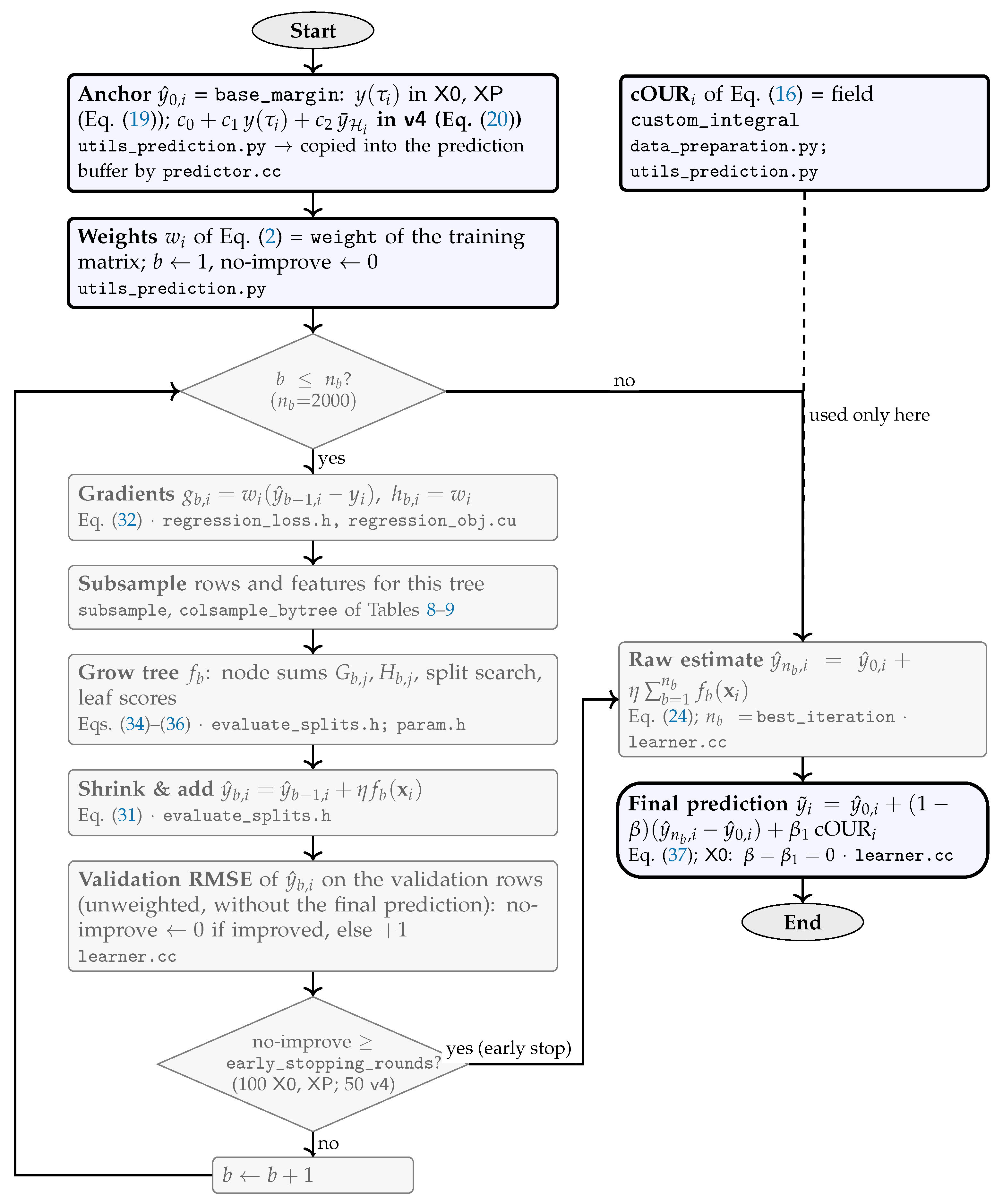
Disclaimer/Publisher’s Note: The statements, opinions and data contained in all publications are solely those of the individual author(s) and contributor(s) and not of MDPI and/or the editor(s). MDPI and/or the editor(s) disclaim responsibility for any injury to people or property resulting from any ideas, methods, instructions or products referred to in the content. |
© 2026 by the authors. Licensee MDPI, Basel, Switzerland. This article is an open access article distributed under the terms and conditions of the Creative Commons Attribution (CC BY) license (http://creativecommons.org/licenses/by/4.0/).
Copyright: This open access article is published under a Creative Commons CC BY 4.0 license, which permit the free download, distribution, and reuse, provided that the author and preprint are cited in any reuse.