

Submitted:
02 October 2026
Posted:
05 October 2026
You are already at the latest version
Abstract
Retrieval of soil organic carbon (SOC) from uncrewed aerial vehicle (UAV) hyperspectral imagery depends on how laboratory measurements are linked to pixels at centimetre resolution. This study presents a quality-controlled workflow in which radiometric calibration, harmonisation against proximal spectroradiometer measurements, pixel-level screening, spectral support definition and model validation are treated as interdependent components of a single procedure. Imagery was acquired with a tunable Fabry–Pérot interferometer camera in six bands between 670 and 1100~nm over eight bare soil fields in Flanders, Belgium (85 topsoil samples) and five fields in Central Macedonia, Greece (42 samples). Single pixel spectra, neighbourhood aggregation and local pixel augmentation were compared at radii of 0.25, 0.50 and 1.00~m using Random Forest, XGBoost, a 1D convolutional neural network and TabPFN, with all pixels from a given sampling location assigned to the same cross-validation fold. In Flanders, 23 of 24 neighbourhood configurations reduced RMSE relative to single pixel extraction, the best reaching \(R^2 = 0.784\) and RMSE =0.155% SOC. In Central Macedonia, adverse acquisition conditions and a narrow target range prevented a usable SOC model, although electrical conductivity, CaCO3 and pH reached \(R^2\) between 0.61 and 0.69. These results indicate that the spectral support should be defined to match the field sampling support, and that this correspondence belongs alongside radiometric calibration, pixel screening and validation in a reproducible workflow for field-scale soil mapping.
Keywords:
UAV hyperspectral
; soil organic carbon
; quality control
; spatial context
; machine learning
1. Introduction
Soil organic carbon (SOC) is a key indicator of soil fertility, agricultural productivity and ecological sustainability [1,2]. It influences nutrient cycling, soil aggregation, water-holding capacity and cation exchange, while also representing an important terrestrial carbon pool [3,4,5]. Spatially explicit information on SOC is therefore relevant for precision agriculture, soil management and carbon-sequestration strategies. Conventional laboratory analysis provides reliable SOC measurements, but collecting samples at the density required for field-scale mapping is costly and time-consuming. Proximal and remote sensing approaches have consequently attracted increasing interest as complementary tools for estimating soil properties over larger areas.
Hyperspectral remote sensing is particularly promising because it records reflectance in many narrow and contiguous spectral bands, allowing subtle variations related to soil composition, mineralogy, moisture, texture and surface condition to be observed [6,7,8,9]. While modern hyperspectral sensors capture vast amounts of data, there is often significant redundancy among contiguous bands, and a carefully selected subset of wavelengths can be sufficient for most soil-property retrievals. In the visible and near-infrared (VNIR) range, SOC-related spectral responses are commonly expressed through broad and overlapping absorption patterns associated with organic matter, soil colour, mineral composition and other soil characteristics that co-vary with carbon content. Compared with multispectral sensors, hyperspectral instruments can preserve more of this information and may therefore support more detailed soil-property retrieval [10]. UAV-borne hyperspectral systems are especially attractive for field-scale applications because they can acquire imagery at centimetre-scale spatial resolution under flexible acquisition conditions. This makes them suitable for heterogeneous and fragmented agricultural fields, where satellite observations may contain mixed pixels (i.e., individual pixels comprising a combination of multiple land cover or surface types) or be unavailable during suitable bare-soil conditions [11].
UAV hyperspectral imagery has been used to estimate a range of soil properties, including salinity, moisture, pH, texture, nitrogen, organic matter and trace elements. However direct UAV hyperspectral studies of soil organic matter (SOM) and SOC remain comparatively limited and reported performance varies substantially among sites. Yan et al. [12] demonstrated field-scale SOM mapping using a small calibration dataset and averaged centimetre-scale spectra within a m support around each sampling location. This approach recognised that a laboratory soil sample is more appropriately represented by a local image neighbourhood than by an individual pixel. Song and Zhang [13] further demonstrated the potential of UAV hyperspectral imagery for SOC mapping across multiple farmland areas, while showing that retrieval accuracy depends strongly on field conditions, spectral preprocessing and modelling choices. Similar sensitivities have been reported for UAV-based estimation of soil texture [14], salinity [15], available copper [16] and heavy metals [17]. Collectively, these studies show that UAV hyperspectral data can support detailed soil-property mapping, but also indicate that image quality, the way spectra are extracted around soil-sampling locations, and validation design are decisive for the credibility of the resulting models and maps.
The reliability of a predictive soil mapping model depends largely on the quality of the spectra extracted at the sampling locations, which imposes challenges with UAV based data acquisition and processing. Due to variable environmental conditions and imperfections in imaging hardware, the UAV hyperspectral data may contain radiometric inconsistencies, geometric misalignment, striping and mosaicking artefacts that introduce spectral variation unrelated to soil properties. If such effects are not identified and mitigated before modelling, learning algorithms may interpret them as meaningful soil variability. Radiometric calibration, geometric processing and systematic image-quality assessment are therefore prerequisites for physically meaningful soil-property prediction rather than preprocessing steps [18].
The confidence to a model outcome depends on how the model performance is evaluated. When multiple pixels are extracted around the same soil-sampling location, these observations are spatially related and cannot be treated as independent samples. Cross-validation must therefore respect the hierarchical structure of the data by keeping all pixel observations associated with a given soil sample within the same validation fold [19]. Evaluation across independent fields is additionally needed when the objective is to assess transferability beyond the calibration setting.
Against this background, this study evaluates a quality-controlled workflow for field-scale prediction of SOC from UAV hyperspectral imagery. It treats image preprocessing, the extraction of spectra around soil-sampling locations, and model validation as interdependent parts of a single workflow rather than isolated technical steps. First, reflectance is radiometrically calibrated, harmonised against colocated proximal spectroradiometer measurements and screened at pixel level before spectra are extracted around the soil-sampling locations. Second, three strategies for relating laboratory observations to high-resolution imagery are compared: single-pixel spectra, neighbourhood-aggregated features and local pixel-level augmentation. Third, all image observations associated with the same soil sample are assigned to the same cross-validation fold to prevent optimistic estimates arising from spatially related pixels. The aim is therefore not only to compare predictive accuracy, but to establish a reproducible and statistically sound procedure for translating sparse soil observations into trustworthy UAV-based field-scale predictions.
2. Materials and Methods
2.1. Overall Workflow
Figure 1 summarises the proposed workflow for quality-controlled UAV hyperspectral soil-property mapping.
2.2. Study Areas, Soil Sampling and Laboratory Analysis
Two agricultural regions with contrasting soil-forming conditions and climate were selected to test the workflow across independent settings.
2.2.1. Flanders Site (Belgium)
The first study area was located in East Flanders, Belgium, in an arable landscape in the municipality Merelbeke-Melle (approximately 10km south-east of Ghent, site center near N, E; UTM zone 31N, EPSG:32631). The region has a temperate maritime climate. Eight sandy-loam bare-soil agricultural fields were surveyed (B2, Caritas, L1, L3, M5B, R6, RvK1A–B and S24), covering a range of field sizes and organic-carbon levels (Table 1).
A total of 85 georeferenced topsoil samples were collected across the eight fields, with between 3 and 27 samples per field depending on field area and expected within-field variability. At each location, a soil sample was taken from the 0–10 cm layer; each sample was a composite of 10 cores within a diameter of approximately 2m. Geo-coordinates of the samples were recorded with a RTK GNSS receiver in WGS84 and subsequently projected to UTM zone 31N to align with the hyperspectral orthomosaics.
2.2.2. Central Macedonia Site (Greece)
The second study area was located in the Region of Central Macedonia, northern Greece, with agricultural fields distributed across the Regional Units of Imathia and Thessaloniki. The area is characterized by a Mediterranean climate with warm, dry summers and cool, wetter winters and comprises a heterogeneous agricultural landscape with a wide range of crop types. The surveyed fields included both annual crops and perennial orchards, predominantly olive and pomegranate orchards, as well as wheat and cotton fields. This diversity provided contrasting field conditions, vegetation structures, and soil-management practices across the study area.
A total of 42 georeferenced topsoil samples were collected across the selected agricultural fields. At each sampling location, soil was collected from the 0–10 cm layer by combining multiple soil subsamples taken within an approximately 2 m radius around the sampling point to obtain a representative composite sample.
2.2.3. Laboratory Analysis
Soil analyses were performed at separate laboratories for the two campaigns, each following its routine protocol. The SOC values of the Flemish samples were analysed at the accredited ILVO soil analysis laboratory by dry combustion following ISO 10694, and they were reported as a mass fraction (% of oven-dry soil). The Central Macedonia samples were air-dried prior to analysis and their SOC values were determined by Walkley–Black wet oxidation. These samples were additionally characterized for particle-size distribution (sand, silt and clay) by the Bouyoucos hydrometer method, for coarse fraction by sieving, for pH by potentiometric method, for electrical conductivity (EC) by conductometric method, for calcium carbonate (CaCO3) by the Bernard calcimeter method, and for total nitrogen (N) by the Kjeldahl method.
Across the Flanders site, measured SOC ranged from 0.86% to 2.14% (mean , median , standard deviation ; coefficient of variation ). Per-field summary statistics are provided in Table 1. Field-level mean SOC ranged from in S24 to in Caritas and M5B.
At the Central Macedonia site, SOC ranged from 0.60% to 1.30%, with a mean of and a standard deviation of . Per-field SOC statistics are reported in Table 2, with field-level means ranging from in PM to in RD. These values indicate a generally lower and narrower SOC range than that observed at the Flanders site.
For the additional soil properties measured in Central Macedonia, sand content ranged from 47 to 59% (mean , standard deviation ), silt content from 23 to 36% (mean , standard deviation ), and clay content from 16 to 21% (mean , standard deviation ). The coarse fraction ranged from 2.0 to 2.7% (mean , standard deviation ), while CaCO3 ranged from 0.8 to 7.0% (mean , standard deviation ). Soil pH varied from 6.98 to 7.61 (mean , standard deviation ), and EC from 408 to 604 S cm−1 (mean S cm−1, standard deviation S cm−1). Total N ranged from 0.30 to 1.10 g kg−1, with a mean of g kg−1 and a standard deviation of g kg−1.
These laboratory values constitute the reference target for model calibration and validation.
2.3. UAV Hyperspectral Acquisition
The spectral imagery was acquired using a tuneable Fabry–Pérot interferometer (FPI) hyperspectral camera developed by VTT. The imager is able record wavelengths from 650 nm to 1200 nm and allows the user to programmatically select the spectral bands to be captured. The imager scans the wavelengths of interest and produces a 2D frame for each spectral band. The images produced by the 1.3 megapixel InGaAs sensor were binned by the camera once horizontally and once vertically to reduce the storage size of the recorded data. The instrument was mounted on a multi-rotor UAV and included a global navigation satellite system (GNSS) receiver for georeferencing the image data. Table 3 shows the key specifications of the imager.
Six bands with center wavelengths of 670, 730, 800, 930, 970 and 1100 nm in the red to near-infrared (VNIR) region were selected for this study. The objective was to obtain the spectral features most relevant to soil organic carbon while limiting acquisition time and data volume. The UAV was operated at 80–100 m altitude above ground level under fair-sky conditions, giving a ground sample distance of approximately 1.1–1.4 cm. Three reference panels of known reflectance (50%, 80% and 95%) were placed within each scene and imaged together with the field; their use for radiometric calibration is described in Section 2.4.
Flights were conducted over the Flanders fields between 19 September and 21 October 2025 and over the Central Macedonia fields between 16 and 27 February 2026. The two campaigns consequently differ in season: the Flemish fields were surveyed post-harvest under bare-soil conditions, whereas the Central Macedonia survey fell within the wet winter period, when autumn-sown cereals were actively growing and orchards carried a permanent canopy. The implications for spectral quality and retrieval performance are considered in Section 4. Per-flight dates and the resulting orthomosaics are available in the archived dataset [20,21]. Acquisitions were generally scheduled as close to local solar noon as practical (13:00-14:00 local time) to minimise variation in illumination geometry, although flight times varied across some fields due to cloud conditions and the limited availability of suitable bare-soil conditions. Because the FPI camera acquires the wavelength bands sequentially rather than simultaneously, a spatial offset arises between bands when the platform is moving; this was addressed by low flight speed. Individual frames were mosaicked into per-field orthomosaics using OpenDroneMap [22].
2.4. Quality Control and Spectral Extraction
The reliability of a predictive model depends on the quality of the spectra acquired, so the spectral extraction step was treated as a modelling decision rather than as preprocessing. This section describes, in the order applied, how reflectance was calibrated and harmonised across sensors, which pixels were considered valid, how vegetation was handled without sacrificing sample size, and how the pixels were related to each laboratory measurement.
2.4.1. Radiometric calibration
The reflectances were calibrated using the signal from the three reference panels of nominal reflectances 0.50, 0.80 and 0.95 imaged within each scene. The mean signal over a manually delineated region on each panel was fit with with zero-offset constrained regression to the nominal reflectance, so that zero signal maps to zero reflectance and a single multiplicative gain per band was obtained. Constraining the intercept avoids the negative reflectances that an unconstrained fit can produce at low signal, at the cost of absorbing any additive path-radiance term into the gain.
For the Central Macedonia campaign, field reference spectra were collected using a PSR+ 3500 spectroradiometer (Spectral Evolution Inc., Lawrence, MA, USA), covering the 350–2500 nm range via a 512-element silicon photodiode array (350–1000 nm; 2.8 nm spectral resolution) and two 256-element InGaAs arrays (970–1910 nm, 8 nm resolution; 1900–2500 nm, 6 nm resolution). Measurements were acquired with a bare fibre under ambient illumination, in nadir orientation matching the UAV viewing geometry, and calibrated against a Spectralon reference panel; PSR acquisitions were performed concurrently with the UAV flights to minimise illumination differences between the two datasets. PSR spectra were resampled to the six UAV band centres and bandwidths by averaging the high-resolution PSR reflectance over each band`s nominal bandwidth prior to comparison with UAV reflectance.
An additional harmonisation step was applied for the Central Macedonia campaign because residual differences remained between panel-calibrated UAV reflectance and colocated PSR measurements. UAV spectra were matched to PSR observations by searching a limited neighbourhood around each PSR coordinate to account for geolocation and orthomosaic misalignment, retaining only spectrally consistent and locally homogeneous candidates. A multiplicative gain was then estimated independently for each band from the ratio of PSR to UAV reflectance and applied uniformly to the corresponding orthomosaic. This step provides an independent, field-based check on the panel calibration specifically at the Central Macedonia site, where residual bias was detected; no comparable PSR deployment was available at the Flanders site, where the panel-based calibration alone was used throughout.
2.4.2. Pixel-Level Validity Criteria
The pixels within each orthomosaic were checked against the following validity criteria. Pixels flagged as no-data were excluded. Any band returning non-positive reflectance was treated as invalid. Due to factors such as sensor noise, vignetting, or data transmission errors, individual spectral bands may occasionally be missing for a given pixel. Because a partial spectrum cannot be used consistently across the derived features, a pixel was discarded entirely if any of the six bands was missing.
2.4.3. Neighbourhood-Based Extraction of UAV Pixels
To link each laboratory measurement with the high-resolution UAV imagery, a circular neighbourhood of radius r was defined around each recorded soil-sampling coordinate This approach avoids relying exclusively on a single nearest pixel, which may be affected by local surface heterogeneity, geolocation uncertainty or image noise. Figure 2 shows representative neighbourhoods over the UAV orthomosaic. Three radii were evaluated, m, corresponding to circular supports of 0.5, 1.0 and 2.0 m diameter.
2.4.4. Vegetation Filtering
The Central Macedonia campaign included perennial orchards and standing annual crops, and therefore fully bare spectral support could not be assumed. NDVI was calculated for each valid pixel as
where and denote the reflectance measured in the bands centred at 800 and 670 nm, respectively.
Rather than applying a fixed NDVI threshold, which can remove different numbers of pixels or even entire sampling locations depending on local vegetation conditions, vegetation influence was reduced using relative NDVI ranking within each sampling neighbourhood. Candidate pixels were ranked in ascending order of NDVI, with distance from the sampling coordinate used to resolve ties. A fixed fraction q of the pixels with the lowest NDVI values was then retained (Figure 3). In this study, was used.
This procedure preferentially retains the least vegetated spectral observations available around each soil sample while avoiding the loss of sampling locations that may occur with an absolute NDVI threshold. No additional vegetation selection was required for the Flanders campaign because imagery was acquired under predominantly bare-soil conditions.
2.4.5. Spectral Extraction Strategies
From this common neighbourhood definition, three strategies for relating the laboratory measurement to the imagery were compared.
- Single-pixel spectra (baseline): The reflectance of the single pixel containing the sampling coordinate was used directly. This represented the conventional point-based extraction and served as the baseline against which the neighbourhood strategies are assessed.
- Neighbourhood-aggregated features: For each sampling location, the per-band mean and standard deviation of reflectance were computed over all selected pixels in the circular neighbourhood, summarising both the average spectral response and its local variability. This yielded a single feature vector, and hence one training observation, per soil sample.
- Local pixel-level augmentation: Every selected pixel within the neighbourhood was treated as an individual training observation, each inheriting the laboratory SOC value of its parent sampling location. This increased the number of pixel-level training instances available to the models while retaining the fine-scale spectral variation within each support. To prevent information leakage, every pixel was tagged with the identifier of its parent sampling location so that all pixels from the same location could be constrained to the same cross-validation fold.
- Derived spectral features: In all strategies, the same set of derived spectral features was appended to the reflectance values: first-order spectral derivatives between consecutive bands, and normalised differences between every pair of bands (), analogous to normalised vegetation indices but applied across the full six-band set. This yielded 26 features per observation for the single-pixel and pixel-augmentation strategies (six reflectances, five derivatives and fifteen normalised differences), and 32 features for the aggregated strategy, which additionally included the six per-band standard deviations. For the aggregated case, the derived indices were computed from the per-band mean reflectances. The feature definition was identical at both study sites.
2.5. Model Development and Validation
Because multiple pixels can originate from the same soil sample, all observations associated with a given sampling location were kept together within the same cross-validation fold. This prevented spatially related pixels from appearing in both training and validation data. Model performance was evaluated using grouped cross-validation.
Four regression algorithms were evaluated: Random Forest (RF) [23], gradient-boosted trees (XGBoost) [24], a one-dimensional convolutional neural network (CNN) [25], and TabPFN [26]. RF and XGBoost were included as established tree-based ensemble methods, while the CNN provided a conventional deep-learning baseline. TabPFN was additionally evaluated as a pretrained transformer-based foundation model for tabular prediction.
The RF model used 200 trees with unlimited depth. The XGBoost model used 200 trees with a learning rate of 0.1, a maximum depth of 4, and subsampling of both observations and features at 0.8. The CNN comprised two one-dimensional convolutional layers (16 and 8 filters, kernel size 3, Leaky-ReLU activation, weight regularisation of ), followed by two fully connected layers (32 and 16 units) and a single linear output. It was trained by minimising the mean squared error with the Adam optimiser (initial learning rate ) for up to 200 epochs with a batch size of 64. Hyperparameters were fixed at these values for all models and were not tuned per field or per strategy, to keep the comparison between extraction strategies unbiased.
Each model was finally retrained using all available observations for each strategy and algorithm to generate wall-to-wall SOC maps for the surveyed fields. All models used fixed random seeds to ensure reproducibility.
2.5.1. Validation Design
Model evaluation was organised at the soil-sampling-location level, matching the independent laboratory reference measurements. Performance was assessed using five-fold cross-validation with a common fold structure across extraction strategies, so that all strategies were evaluated on identical held-out sampling units. For pixel-level augmentation, all pixels from a given sampling location were assigned to the same fold, and their held-out predictions were averaged to the sampling-location level before any performance metric was computed. Predictive performance was quantified using RMSE and on the pooled out-of-fold predictions.
2.5.2. Statistical Significance Testing
The purpose of the significance testing was to determine, for each soil property and regression model, whether replacing single-pixel extraction with a spatially-informed extraction strategy produced a reduction in prediction error that reflects a genuine effect of incorporating spatial context, rather than variability attributable to the specific cross-validation split.
Each extraction configuration (a strategy–radius combination) was therefore compared against the single-pixel baseline of the same regression model on the same paired sample-level out-of-fold predictions, using an identical procedure applied uniformly across the full design: this comparison is the basic unit of inference, repeated once per property, model, strategy and radius. The null hypothesis, common to every such comparison, is that the baseline and method predictions are exchangeable with respect to the true value at each sampling location. This was tested with a paired permutation test on the RMSE difference, which avoids assuming a parametric error distribution and accommodates RMSE as a non-linear aggregate statistic; 95% confidence intervals for the RMSE difference were obtained by paired bootstrap resampling of the sampling locations.
Every configuration for a given property and model was tested against the same baseline. These comparisons therefore form a single family of hypotheses per property–model combination. Raw p-values were adjusted within each such family using the Holm step-down procedure [27] at , so that the reported significance controls the family-wise probability of at least one false positive among the configurations compared for that model.
3. Results
3.1. Comparison of Spectral Extraction Strategies
Table 4 summarises SOC prediction performance at the Flanders site across the three spectral extraction strategies, neighbourhood radii and regression models. RMSE reduction is expressed relative to the corresponding single-pixel baseline for each model, while the reported Holm-adjusted p-values quantify the significance of the paired improvement over that baseline.
The single-pixel strategy provided moderate predictive performance for RF, XGBoost and TabPFN, with values between 0.467 and 0.498 and RMSE values between 0.236 and 0.244 % SOC. In contrast, the CNN performed worse than other models when trained from a single pixel per sampling location (, RMSE % SOC), indicating greater sensitivity to the limited point-based spectral representation.
Neighbourhood aggregation improved SOC prediction for most combinations of radius and regression model. For RF, XGBoost and TabPFN, performance generally increased as the neighbourhood radius increased. The best overall configuration was obtained with TabPFN using aggregated features at a radius of 1.0 m, reaching and RMSE % SOC. This corresponded to a 36.5% reduction in RMSE relative to the TabPFN single-pixel baseline (). RF and XGBoost showed similar improvements at 1.0 m, reaching and , respectively. The effect of aggregation was less consistent for the CNN, with performance improving at 0.25 and 0.50 m but deteriorating at 1.0 m.
Pixel-level augmentation produced a more consistent improvement across models. All augmentation configurations reduced RMSE relative to their corresponding single-pixel baselines and remained significant after Holm correction. The strongest augmented results were obtained at the larger neighbourhood sizes: at 1.0 m, RF, XGBoost and TabPFN reached values of 0.754, 0.749 and 0.763, respectively, with RMSE reductions of approximately 29–33%. The CNN benefited particularly from augmentation, reaching its best performance at 0.50 m (, RMSE % SOC), corresponding to a 37.0% reduction in RMSE relative to its single-pixel baseline.
Overall, 23 of the 24 neighbourhood-based configurations reduced RMSE relative to the corresponding single-pixel model, and 20 remained significant after Holm correction. Although no single extraction strategy was uniformly superior across all models and radii, the results consistently demonstrate the benefit of incorporating spatial context around the soil-sampling location. Larger neighbourhoods generally provided the strongest performance, although this relationship was model dependent and not strictly monotonic.
In Central Macedonia, SOC prediction was substantially more difficult than in Flanders. Because any combination of the used extraction strategy, used radius, and used algorithm did not produce a reliable model, Table 5 reports the best-performing configuration per strategy, selected by lowest pooled out-of-fold RMSE. Neighbourhood augmentation produced a numerical improvement, with the best configuration reaching and RMSE % SOC, close to the site standard deviation of 0.19 %, but the improvement was not significant after Holm correction (). As even these best cases show no usable predictive skill, the remaining configurations do not affect any conclusion drawn here.
3.2. Generalization to Additional Soil Properties in Central Macedonia
The same neighbourhood-based framework was subsequently evaluated for the additional soil properties available in Central Macedonia. The clearest improvements were observed for EC and CaCO3, for which pixel-level augmentation at a 1.0 m radius produced substantial reductions in prediction error. For EC, the best configuration was obtained with RF (, RMSE ), corresponding to a 38.5% reduction in RMSE relative to the closest-pixel baseline (). For CaCO3, TabPFN with augmentation at 1.0 m achieved and RMSE , representing a 29.2% reduction in RMSE ().
For pH, the lowest prediction error was obtained with CNN augmentation at 1.0 m (, RMSE ). Although this corresponded to a large 91.3% reduction relative to the same-model closest-pixel baseline, the magnitude of the relative improvement should be interpreted cautiously because the CNN baseline performed poorly. Prediction also remained weak for clay and total N, with the best configurations yielding values close to or below zero.

Table 6.
Best-performing neighbourhood-based configuration for each soil property. RMSE improvement is calculated relative to the corresponding closest-pixel baseline using the same regression model.
Table 6.
Best-performing neighbourhood-based configuration for each soil property. RMSE improvement is calculated relative to the corresponding closest-pixel baseline using the same regression model.
| Property | Model | Strategy | Radius (m) | RMSE | RMSE improvement (%) | ||
|---|---|---|---|---|---|---|---|
| CaCO3 | TabPFN | Augmentation | 1.00 | 0.625 | 1.119 | 29.2 | 0.0036 |
| Clay | XGBoost | Augmentation | 0.50 | 0.042 | 1.308 | 7.8 | 1.0000 |
| EC | RF | Augmentation | 1.00 | 0.686 | 28.13 | 38.5 | 0.0010 |
| N | TabPFN | Aggregation | 0.25 | -0.069 | 0.235 | -0.4 | 0.8710 |
| pH | CNN | Augmentation | 1.00 | 0.609 | 0.115 | 91.3 | 0.00024 |
4. Discussion
The results show that the way UAV spectra are associated with laboratory measurements can substantially influence soil property prediction. Both the neighbourhood aggregation and the pixel-level augmentation improved the SOC prediction results in the favourable bare soil conditions in Flanders. Most neighbourhood-based configurations performed significantly better than their corresponding single-pixel baselines after Holm correction, supporting the overall benefit of incorporating spatial context. There was not however a consistently superior strategy across all models and different neighborhoud sizes. This indicates that the main finding is not optimizing a universal model but the value of incorporating spatial context surrounding each location.
This benefit can largely be explained by the difference in the area that the imagery and the laboratory measurements represent. Each laboratory value originates out of a composite sample collected from several subsamples within a local area, whereas a single UAV pixel represents only a small portion of that area. Neighbourhood-based extraction made the spectral representation of the imagery more consistent with the soil measurements. Aggregation may additionally reduce sensitivity to positional errors, micro scale variability and residual radiometric or mosaicking artifacts. The general improved performance at larger neighbourhood sizes supports this interpretation although the relationship was not strictly monotonic and remained dependent on the model and the extraction strategy.
Aggregation and augmentation incorporated spatial context in different ways. Aggregation reduced local spectral variability into a single representation for each sampling location, while the inclusion of per-band standard deviations retained some information about neighbourhood heterogeneity. Augmentation instead preserved the individual pixel spectra and allowed the models to learn from their local variation. The positive results obtained through aggregation also indicate that increasing the number of training observations is not always preferable to construct a more stable representation of each soil sample. Thus the aggregation offers practical benefit in terms of training time, memory requirements, and energy efficiency. Augmentation may nevertheless be particularly valuable for future large-scale deep-learning approaches capable of exploiting the increased number and diversity of pixel-level training instances.
The considerably weaker SOC results in Central Macedonia suggest that the extraction strategies could not overcome the limitations affecting SOC prediction at this site. This dataset was smaller and covered a narrower SOC range (Table 5) providing the models with less independent information and less target variability in order to learn a stable relationship. The hyperspectral acquisitions being in winter introduced further difficulties. Several fields were humid and contained growing vegetation, while the olive orchards had permanent canopies. Soil moisture can strongly modify soil reflectance and potentially mask SOC related spectral response while vegetation reduces the availability of representative exposed soil pixels. These factors probably contributed to the contrasting results with the optimal post harvest bare soil conditions in Flanders.
The relative NDVI-ranking procedure provided a consistent way of identifying the least vegetation-affected pixels under heterogeneous field conditions. Spectral-index thresholding can be highly sensitive to the selected threshold [28], and no single value could be applied across all samples without excluding an excessive number of pixels in some cases. Relative ranking was therefore less dependent on site-specific reflectance conditions. However, in neighbourhoods already dominated by bare soil, it may discard some valid bare-soil pixels. This represents a trade-off between retaining all potentially valid pixels and applying a consistent selection strategy less sensitive to local heterogeneous conditions.
These limitations did not affect all soil properties equally. Neighbourhood-based modelling improved the prediction of EC, CaCO3, and pH, which indicates that local spatial context captured useful soil-related information even under challenging acquisition conditions. This could further indicate that these properties exhibited stronger spatial variation than SOC or stronger associations with the measured spectra than SOC. While properties such as pH and EC are commonly estimated through associations with mineral composition, moisture and other soil characteristics [29,30], several important mineral and carbonate absorption features occur at longer wavelengths than those used in this study, which may explain why clay content and total nitrogen remained difficult to predict. Therefore, the successful predictions likely reflect a combination of indirect spectral information and spatial covariation within the surveyed fields.
Radiometric calibration, cross-sensor harmonisation and pixel screening are preconditions for the reflectance values to carry physical meaning and their role is to establish the conditions under which the spectral support is reliable. The validation design and use of fixed model configurations enabled a consistent comparison of the extraction strategies which was the main objective of this study. All pixels associated with one location were kept within the same cross-validation fold, and their predictions were combined at each point, preventing information leakage from pixels sharing the same laboratory measurement. Since the strategies were evaluated at the same test locations, local factors such as soil conditions and illumination were also shared, focusing the comparison on the effect of spectral extraction. It must be emphasized that the performed evaluation does not provide any evidence for model generalization or transferability to other geographical areas. To achieve this, a different test setup is needed; this, however, is outside the scope of this study. Per-field sample counts (Table 1) were in any case too small to test the models reliably on unseen fields. Finally, part of the performance improvement observed for the neighbourhood-based strategies likely reflects spatial coherence within a field, such as local homogeneity in soil condition, alongside a physical relationship between reflectance and SOC.
The findings should be interpreted within the experimental scope of the study. The number of independent soil samples was limited, particularly in Central Macedonia, and augmentation increased the number of pixel-level training instances rather than the number of laboratory measurements. Although these six bands were deliberately selected to target primary SOC-related features, this restricted the spectral information available for modelling some soil properties. Because acquiring more bands increases data volume and acquisition time, this band configuration was a deliberate trade-off to maximize flight endurance (flight time per battery) for a UAV-borne FPI system operating within the VNIR range; extending the wavelength range into the SWIR, where several mineral and carbonate absorption features are more pronounced, would require a different sensor class and is outside the spectral range of the instrument evaluated here. Future work should extend the workflow through additional campaigns covering a wider range of soils, crops, seasons and surface conditions. Data-fusion strategies linking centimetre-resolution UAV observations with satellite imagery could support the upscaling of field-level predictions to regional applications. Federated learning could further support collaborative modelling across campaigns, institutions and geographical regions while reducing the need to centralise raw field data or precise sampling coordinates [31].
Taken together, these findings show that the spatial relationship between UAV imagery and field measurements is a central component of soil-property modelling. Neighbourhood-based representations improved upon single-pixel extraction under favourable bare-soil conditions and captured useful information for several properties under more challenging conditions. Spatial context should therefore be considered as an integral part of the modelling workflow along radiometric calibration, pixel screening and statistically sound validation.
5. Conclusions
This study developed and evaluated a quality-controlled workflow for converting UAV imagery (acquired using six selected bands of a tunable FPI hyperspectral sensor) and laboratory measurements into field-scale predictions of SOC and related soil properties. The workflow combined radiometric calibration and harmonisation, pixel screening, alternative spectral extraction strategies and statistically sound validation. In Flanders, both neighbourhood aggregation and pixel-level augmentation improved SOC prediction over single-pixel extraction across multiple regression models, achieving an R² of up to 0.784. In Central Macedonia, none of the evaluated configurations produced a reliable SOC model, although neighbourhood-based extraction improved the prediction of EC, CaCO3 and pH, while clay and total nitrogen remained difficult to predict.
These results demonstrate that incorporating spatial context can improve the model performance when using of centimetre-resolution UAV imagery, but it cannot compensate if the imagery or reference dataset do not contain sufficient information about the target property. Reliable UAV-based soil mapping therefore depends on the complete workflow rather than on regression-model selection alone, including image quality, the correspondence between spectral extraction and field sampling, and validation that preserves the independence of sampling locations. The proposed workflow provides a reproducible basis for field-scale soil-property mapping with tunable UAV hyperspectral sensors and for further evaluation across additional campaigns and broader spectral ranges.
References
- Stockmann, U.; Adams, M.A.; Crawford, J.W.; Field, D.J.; Henakaarchchi, N.; Jenkins, M.; Minasny, B.; McBratney, A.B.; de Remy de Courcelles, V.; Singh, K.; et al. The knowns, known unknowns and unknowns of sequestration of soil organic carbon. Agriculture, Ecosystems & Environment 2013, 164, 80–99. [CrossRef]
- Lefèvre, C.; Rekik, F.; Alcantara, V.; Wiese, L. Soil organic carbon: the hidden potential.; Food and Agriculture Organization of the United Nations (FAO): Rome, 2017; pp. ix + 77 pp.
- Lal, R. Soil Carbon Sequestration Impacts on Global Climate Change and Food Security. Science 2004, 304, 1623–1627, [https://www.science.org/doi/pdf/10.1126/science.1097396]. [CrossRef]
- Cotrufo, M.F.; Lavallee, J.M. Chapter One - Soil organic matter formation, persistence, and functioning: A synthesis of current understanding to inform its conservation and regeneration; Academic Press, 2022; Vol. 172, Advances in Agronomy, pp. 1–66. [CrossRef]
- Zhou, Z.; Ren, C.; Wang, C.; et al. Global Turnover of Soil Mineral-Associated and Particulate Organic Carbon. Nature Communications 2024, 15, 5329. [CrossRef]
- Ben-Dor, E.; Chabrillat, S.; Demattê, J.; Taylor, G.; Hill, J.; Whiting, M.; Sommer, S. Using Imaging Spectroscopy to study soil properties. Remote Sensing of Environment 2009, 113, S38–S55. Imaging Spectroscopy Special Issue, . [CrossRef]
- Bhargava, A.; Sachdeva, A.; Sharma, K.; Alsharif, M.H.; Uthansakul, P.; Uthansakul, M. Hyperspectral imaging and its applications: A review. Heliyon 2024, 10, e33208. [CrossRef]
- Stenberg, B.; Viscarra Rossel, R.A.; Mouazen, A.M.; Wetterlind, J. Chapter Five - Visible and Near Infrared Spectroscopy in Soil Science; Academic Press, 2010; Vol. 107, Advances in Agronomy, pp. 163–215. [CrossRef]
- Hosseinpour-Zarnaq, M.; Omid, M.; Sarmadian, F.; Ghasemi-Mobtaker, H.; Alimardani, R.; Bohlol, P. Exploring the capabilities of hyperspectral remote sensing for soil texture evaluation. Ecological Informatics 2025, 90, 103336. [CrossRef]
- Castaldi, F.; Palombo, A.; Santini, F.; Pascucci, S.; Pignatti, S.; Casa, R. Evaluation of the Potential of the Current and Forthcoming Multispectral and Hyperspectral Imagers to Estimate Soil Texture and Organic Carbon. Remote Sensing of Environment 2016, 179, 54–65. [CrossRef]
- Ampas, H.; Karyotis, K.; Guillevic, P.; Zalidis, G.; Petridou, S. Cross-Scale Validation of Hyperspectral Unmixing Over Agricultural Landscapes. IEEE Geoscience and Remote Sensing Letters 2026, 23, 2503005–2503005. [CrossRef]
- Yan, Y.; Yang, J.; Li, B.; Qin, C.; Ji, W.; Xu, Y.; Huang, Y. High-Resolution Mapping of Soil Organic Matter at the Field Scale Using UAV Hyperspectral Images with a Small Calibration Dataset. Remote Sensing 2023, 15, 1433. [CrossRef]
- Song, Q.; Zhang, W. Estimation and Spatial Distribution of Soil Organic Carbon Content in Farmland Using Unmanned Aerial Vehicle Hyperspectral Remote Sensing Technology. Scientific Reports 2026, 16, 5480. [CrossRef]
- Song, Q.; Gao, X.; Song, Y.; Li, Q.; Chen, Z.; Li, R.; Zhang, H.; Cai, S. Estimation and Mapping of Soil Texture Content Based on Unmanned Aerial Vehicle Hyperspectral Imaging. Scientific Reports 2023, 13, 14097. [CrossRef]
- Hu, J.; Peng, J.; Zhou, Y.; Xu, D.; Zhao, R.; Jiang, Q.; Fu, T.; Wang, F.; Shi, Z. Quantitative Estimation of Soil Salinity Using UAV-Borne Hyperspectral and Satellite Multispectral Images. Remote Sensing 2019, 11, 736. [CrossRef]
- Zhang, Y.; Wei, L.; Lu, Q.; Zhong, Y.; Yuan, Z.; Wang, Z.; Li, Z.; Yang, Y. Mapping soil available copper content in the mine tailings pond with combined simulated annealing deep neural network and UAV hyperspectral images. Environmental Pollution 2023, 320, 120962. [CrossRef]
- Chen, H.W.; Chen, C.Y.; Nguyen, K.L.P.; Chen, B.J.; Tsai, C.H. Hyperspectral Sensing of Heavy Metals in Soil by Integrating AI and UAV Technology. Environmental Monitoring and Assessment 2022, 194, 518. [CrossRef]
- Honkavaara, E.; Saari, H.; Kaivosoja, J.; Pölönen, I.; Hakala, T.; Litkey, P.; Mäkynen, J.; Pesonen, L. Processing and Assessment of Spectrometric, Stereoscopic Imagery Collected Using a Lightweight UAV Spectral Camera for Precision Agriculture. Remote Sensing 2013, 5, 5006–5039. [CrossRef]
- Roberts, D.R.; Bahn, V.; Ciuti, S.; Boyce, M.S.; Elith, J.; Guillera-Arroita, G.; Hauenstein, S.; Lahoz-Monfort, J.J.; Schröder, B.; Thuiller, W.; et al. Cross-Validation Strategies for Data with Temporal, Spatial, Hierarchical, or Phylogenetic Structure. Ecography 2017, 40, 913–929. [CrossRef]
- Berkvens, N.; Coppens, T.; Bauwens, J.; Chalazas, T.; De Man, W.; Van Beek, J.; Callens, B.; Van Gehuchten, A.; Kokka, A. Hyperspectral Drone Imagery: Bare Soil Fields, 2026. [CrossRef]
- Ampas, H.; Liakopoulos, V.; Karyotis, K.; Zalidis, G. Hyperspectral UAV imagery of Agricultural Fields, 2026. [CrossRef]
- OpenDroneMap Authors. ODM – A command line toolkit to generate maps, point clouds, 3D models and DEMs from drone, balloon or kite images. https://github.com/OpenDroneMap/ODM, 2020. OpenDroneMap/ODM GitHub Page.
- Breiman, L. Random Forests. Machine Learning 2001, 45, 5–32. [CrossRef]
- Chen, T.; Guestrin, C. XGBoost: A Scalable Tree Boosting System. In Proceedings of the Proceedings of the 22nd ACM SIGKDD International Conference on Knowledge Discovery and Data Mining, New York, NY, USA, 2016; KDD ’16, p. 785–794. [CrossRef]
- Tsakiridis, N.L.; Keramaris, K.D.; Theocharis, J.B.; Zalidis, G.C. Simultaneous prediction of soil properties from VNIR-SWIR spectra using a localized multi-channel 1-D convolutional neural network. Geoderma 2020, 367, 114208. [CrossRef]
- Hollmann, N.; Müller, S.; Purucker, L.; Krishnakumar, A.; Körfer, M.; Hoo, S.B.; Schirrmeister, R.T.; Hutter, F. Accurate predictions on small data with a tabular foundation model. Nature 2025, 637, 319–326. [CrossRef]
- Holm, S. A Simple Sequentially Rejective Multiple Test Procedure. Scandinavian Journal of Statistics 1979, 6, 65–70.
- Ampas, H.; Karyotis, K.; Zalidis, G.; Petridou, S. Spectral Unmixing for Bare Soil Detection: A Step Toward Soil Organic Carbon Estimation. In Proceedings of the 2025 International Conference on Machine Intelligence for GeoAnalytics and Remote Sensing (MIGARS), 2025, pp. 1–4. [CrossRef]
- Karyotis, K.; Ampas, H.; Chatzimisios, P.; Zalidis, G. Fuzzy Cluster Membership as a Reliability Indicator for Continental Soil Spectroscopy Models. Frontiers in Environmental Science 2026, 14. [CrossRef]
- Lukas, V.; Neudert, L.; Novák, J.; Křen, J. Estimation of Soil Physico-chemical Properties by On-the-go Measurement of Soil Electrical Conductivity. Agriculturae Conspectus Scientificus 2018, 83, 93–98.
- Tsakiridis, N.L.; Kalopesa, E.; Zalidis, G.C.; Tziolas, N.; Berkvens, N.; Chalazas, T.; Coppens, T.; Ilias, P. Privacy-Preserving Soil Data: Federated Learning for Topsoil Descriptors Via Remote Sensing. In Proceedings of the IGARSS 2025 - 2025 IEEE International Geoscience and Remote Sensing Symposium, 2025, pp. 640–644. [CrossRef]
Figure 1.
Overview of the quality-controlled UAV hyperspectral workflow for soil organic carbon (SOC) mapping. Laboratory SOC values from composite topsoil samples provide the regression target; UAV imagery is radiometrically calibrated, harmonised against proximal spectroradiometer (PSR) measurements, and screened at pixel level before spectra are extracted within a circular support of radius r around each sampling coordinate. Three extraction strategies are compared: (A) single-pixel, (B) neighbourhood aggregation and (C) pixel-level augmentation. Asterisks mark steps applied at the Central Macedonia site only.
Figure 1.
Overview of the quality-controlled UAV hyperspectral workflow for soil organic carbon (SOC) mapping. Laboratory SOC values from composite topsoil samples provide the regression target; UAV imagery is radiometrically calibrated, harmonised against proximal spectroradiometer (PSR) measurements, and screened at pixel level before spectra are extracted within a circular support of radius r around each sampling coordinate. Three extraction strategies are compared: (A) single-pixel, (B) neighbourhood aggregation and (C) pixel-level augmentation. Asterisks mark steps applied at the Central Macedonia site only.
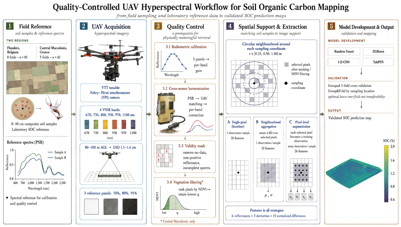
Figure 2.
Representative UAV RGB orthomosaic showing circular neighbourhoods (white) centred on soil sampling locations (red) at the Central Macedonia site (Greece). Pixels within a neighbourhood of radius r were considered for local spectral aggregation and pixel-level augmentation.
Figure 2.
Representative UAV RGB orthomosaic showing circular neighbourhoods (white) centred on soil sampling locations (red) at the Central Macedonia site (Greece). Pixels within a neighbourhood of radius r were considered for local spectral aggregation and pixel-level augmentation.
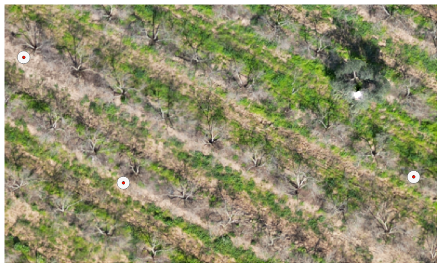
Figure 3.
Neighbourhood-based pixel selection around a soil sampling location. Candidate pixels are first identified within radius r. Pixels excluded by the validity mask are then removed before spectral aggregation or pixel-level augmentation.
Figure 3.
Neighbourhood-based pixel selection around a soil sampling location. Candidate pixels are first identified within radius r. Pixels excluded by the validity mask are then removed before spectral aggregation or pixel-level augmentation.
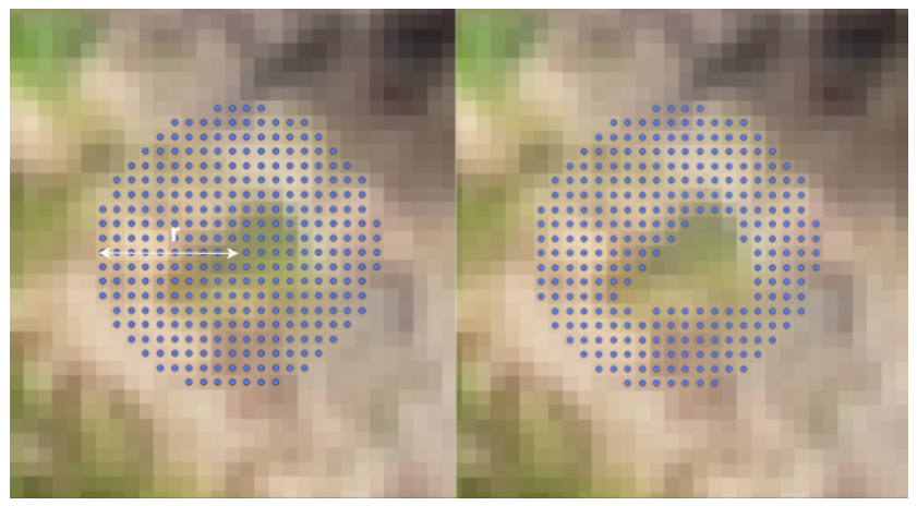
Table 1.
Soil sampling and measured organic-carbon (SOC) content per field at the Flanders study site. SOC is expressed as a mass fraction (% of oven-dry soil).
Table 1.
Soil sampling and measured organic-carbon (SOC) content per field at the Flanders study site. SOC is expressed as a mass fraction (% of oven-dry soil).
| Field | n | Min (%) | Max (%) | Mean (%) | SD (%) |
|---|---|---|---|---|---|
| B2 | 10 | 0.86 | 1.36 | 1.13 | 0.13 |
| Caritas | 27 | 1.40 | 2.14 | 1.75 | 0.20 |
| L1 | 10 | 0.92 | 1.24 | 1.04 | 0.10 |
| L3 | 3 | 1.19 | 1.60 | 1.38 | 0.21 |
| M5B | 7 | 1.59 | 1.90 | 1.75 | 0.12 |
| R6 | 11 | 1.08 | 1.48 | 1.21 | 0.12 |
| RvK1A–B | 14 | 1.04 | 1.65 | 1.35 | 0.23 |
| S24 | 3 | 0.87 | 1.00 | 0.93 | 0.07 |
| All fields | 85 | 0.86 | 2.14 | 1.41 | 0.34 |
Table 2.
Soil sampling and measured soil organic carbon (SOC) content per field at the CM study site. SOC is expressed as a mass fraction (% of oven-dry soil).
Table 2.
Soil sampling and measured soil organic carbon (SOC) content per field at the CM study site. SOC is expressed as a mass fraction (% of oven-dry soil).
| Field | n | Min (%) | Max (%) | Mean (%) | SD (%) |
|---|---|---|---|---|---|
| AP | 4 | 0.70 | 1.10 | 0.88 | 0.21 |
| ELG | 12 | 0.70 | 1.20 | 0.89 | 0.18 |
| GK | 9 | 0.70 | 1.30 | 0.97 | 0.24 |
| PM | 14 | 0.60 | 0.90 | 0.76 | 0.09 |
| RD | 3 | 0.90 | 1.20 | 1.03 | 0.15 |
| All fields | 42 | 0.60 | 1.30 | 0.87 | 0.19 |
Table 3.
Key specifications of the VTT hyperspectral imager used in the study.
| Parameter | Value |
|---|---|
| Sensor technology | InGaAs |
| Pixel resolution | 1280 x 1024 (before 2 x 2 binning) |
| Pixel size | 5 µm (10 µm binned) |
| Field of view | 10.5∘ x 8.4∘ |
| Wavelength range | 650–1200 nm |
| Spectral bandwidth | 30–35 nm |
| FPI aperture diameter | 43 mm |
| Focal length | 35 mm |
| f/N | 1.8 |
| Mass | 1.7 kg |
Table 4.
SOC prediction performance at the Flanders site across spectral extraction strategies, neighbourhood radii and regression models. RMSE reduction is calculated relative to the corresponding same-model single-pixel baseline. Holm-adjusted p-values refer to paired comparisons with that baseline. Positive RMSE reduction values indicate improved prediction performance.
Table 4.
SOC prediction performance at the Flanders site across spectral extraction strategies, neighbourhood radii and regression models. RMSE reduction is calculated relative to the corresponding same-model single-pixel baseline. Holm-adjusted p-values refer to paired comparisons with that baseline. Positive RMSE reduction values indicate improved prediction performance.
| Strategy | Radius (m) | Model | RMSE (% SOC) | RMSE reduction (%) | ||
|---|---|---|---|---|---|---|
| Single pixel | – | RF | 0.491 | 0.238 | – | – |
| – | XGBoost | 0.498 | 0.236 | – | – | |
| – | CNN | -0.157 | 0.359 | – | – | |
| – | TabPFN | 0.467 | 0.244 | – | – | |
| Aggregation | 0.25 | RF | 0.628 | 0.204 | 14.3 | 0.024 |
| 0.25 | XGBoost | 0.607 | 0.209 | 11.1 | 0.126 | |
| 0.25 | CNN | 0.085 | 0.319 | 11.1 | 0.416 | |
| 0.25 | TabPFN | 0.738 | 0.171 | 29.9 | 0.002 | |
| 0.50 | RF | 0.695 | 0.184 | 22.7 | 0.003 | |
| 0.50 | XGBoost | 0.666 | 0.193 | 18.2 | 0.027 | |
| 0.50 | CNN | 0.195 | 0.299 | 16.7 | 0.157 | |
| 0.50 | TabPFN | 0.757 | 0.165 | 32.4 | 0.002 | |
| 1.00 | RF | 0.708 | 0.180 | 24.4 | 0.002 | |
| 1.00 | XGBoost | 0.754 | 0.165 | 30.1 | 0.001 | |
| 1.00 | CNN | -0.573 | 0.418 | -16.4 | 0.416 | |
| 1.00 | TabPFN | 0.784 | 0.155 | 36.5 | 0.001 | |
| Augmentation | 0.25 | RF | 0.704 | 0.182 | 23.5 | 0.003 |
| 0.25 | XGBoost | 0.693 | 0.185 | 21.6 | 0.003 | |
| 0.25 | CNN | 0.427 | 0.253 | 29.5 | 0.006 | |
| 0.25 | TabPFN | 0.690 | 0.186 | 23.8 | 0.024 | |
| 0.50 | RF | 0.734 | 0.170 | 28.6 | 0.001 | |
| 0.50 | XGBoost | 0.735 | 0.172 | 27.1 | 0.001 | |
| 0.50 | CNN | 0.540 | 0.226 | 37.0 | 0.002 | |
| 0.50 | TabPFN | 0.748 | 0.168 | 31.1 | 0.002 | |
| 1.00 | RF | 0.754 | 0.166 | 30.2 | 0.001 | |
| 1.00 | XGBoost | 0.749 | 0.167 | 29.2 | 0.001 | |
| 1.00 | CNN | 0.488 | 0.239 | 33.4 | 0.006 | |
| 1.00 | TabPFN | 0.763 | 0.163 | 33.2 | 0.001 |
Table 5.
Best-performing SOC configuration within each spectral extraction strategy at the Central Macedonia site, selected according to the lowest pooled out-of-fold RMSE. RMSE reduction and Holm-adjusted p-values are calculated relative to the corresponding same-model single-pixel baseline.
Table 5.
Best-performing SOC configuration within each spectral extraction strategy at the Central Macedonia site, selected according to the lowest pooled out-of-fold RMSE. RMSE reduction and Holm-adjusted p-values are calculated relative to the corresponding same-model single-pixel baseline.
| Strategy | Radius (m) | Model | RMSE (% SOC) | RMSE reduction (%) | ||
|---|---|---|---|---|---|---|
| Single pixel | – | TabPFN | -0.066 | 0.194 | – | – |
| Aggregation | 1.00 | RF | 0.048 | 0.183 | 10.0 | 1.000 |
| Augmentation | 0.50 | CNN | 0.106 | 0.177 | 30.9 | 0.501 |
Disclaimer/Publisher’s Note: The statements, opinions and data contained in all publications are solely those of the individual author(s) and contributor(s) and not of MDPI and/or the editor(s). MDPI and/or the editor(s) disclaim responsibility for any injury to people or property resulting from any ideas, methods, instructions or products referred to in the content. |
© 2026 by the authors. Licensee MDPI, Basel, Switzerland. This article is an open access article distributed under the terms and conditions of the Creative Commons Attribution (CC BY) license (http://creativecommons.org/licenses/by/4.0/).
Copyright: This open access article is published under a Creative Commons CC BY 4.0 license, which permit the free download, distribution, and reuse, provided that the author and preprint are cited in any reuse.