

Submitted:
01 October 2026
Posted:
05 October 2026
You are already at the latest version
Abstract
Transformer-based analysis of physiological signals depends critically on how input tokens are constructed, yet conventional tokens derived from raw temporal windows or spectrogram patches may overlook the intrinsic oscillatory organization of electroencephalographic (EEG) activity. To address this limitation, we propose AMST-Former, an adaptive mode-wise synchrosqueezing Transformer for patient-independent epileptic seizure detection. Each EEG channel is first decomposed into oscillatory modes using Adaptive Local Iterative Filtering (ALIF), after which the Synchrosqueezing Transform (SST) is applied independently to each mode. This decomposition-before-synchrosqueezing strategy reduces cross-component interference in instantaneous-frequency estimation while preserv- ing mode-specific time–frequency dynamics. The resulting time–frequency patches are embedded together with channel, mode-frequency, and positional information. A hierarchical factorized-attention mechanism then models token relevance across time–frequency regions, oscillatory modes, and EEG channels before a Transformer encoder captures their interactions. Evaluation using a repeated patient-independent five-fold cross-validation protocol on the CHB-MIT database (22 subjects) yielded an F1-score of 70.76% and an area under the precision–recall curve (AUPRC) of 0.870. At the event level, AMST-Former achieved a sensitivity of 81.4% at one false detection per 24 h. Ablation experi- ments showed that mode-wise SST provided more effective representations than direct SST, per-mode Hilbert spectra, and fixed filter-bank decomposition. Furthermore, the factorized-attention mechanism provides mode, time–frequency, and channel-level explanations, whose faithfulness was assessed through deletion analysis. These results support adaptive mode-wise time–frequency tokenization as a promising strategy for interpretable, patient-independent EEG seizure detection.
Keywords:
explainable artificial intelligence
; representation learning
; tokenization
; transformer
; hierarchical attention
; electroencephalography
; seizure detection
; adaptive local iterative filtering
; synchrosqueezing transform
; patient-independent evaluation
1. Introduction
Epilepsy affects more than 45 million people worldwide and remains one of the leading causes of neurological disability [1,2]. Scalp electroencephalography (EEG) is the reference modality for its diagnosis and monitoring, because it records the abnormal neuronal synchronization that underlies seizures with millisecond resolution and at low cost. In epilepsy monitoring units, however, recordings routinely span several days and dozens of channels, and their visual review by trained neurophysiologists is slow, costly and subject to inter-rater variability. Automated seizure detection is therefore a long-standing objective of clinical neuroengineering [3,4,5].
Two properties of the EEG make this objective difficult. First, the signal is nonstationary and multicomponent: an ictal discharge typically appears as a rhythmic oscillation whose frequency drifts over seconds, superimposed on background rhythms, artifacts and slow trends, and these components frequently overlap in time and frequency. Second, ictal patterns differ markedly from one patient to another. A detector that performs well on segments drawn at random from patients already seen during training may fail on a new patient, and random segment-level splits are known to inflate reported performance substantially [6]. The clinically meaningful question is thus how well a detector generalizes to unseen patients, preferably assessed with event-level criteria that reflect how alarms are used in practice [7].
The representation from which a detector learns largely determines how it copes with the first property. Fixed time–frequency (TF) transforms such as the short-time Fourier and wavelet transforms have been used extensively [8,9,10], but their resolution is bounded by the choice of window or mother wavelet. Data-driven decompositions avoid a predefined basis by splitting the signal into intrinsic mode functions (IMFs), each carrying a single locally defined oscillation. Empirical mode decomposition (EMD) [11] and its noise-assisted variants [12,13] opened this line of work but suffer from mode mixing and lack a solid mathematical foundation [14]. Iterative filtering replaces the heuristic sifting of EMD with convolution-based moving averages [15], and its adaptive extension, Adaptive Local Iterative Filtering (ALIF), lets the filter length follow the local time scale of the signal, which makes it well suited to oscillations whose frequency changes quickly [16,17]. A third line of work sharpens the TF plane itself. The synchrosqueezing transform (SST) reassigns wavelet coefficients from scale to instantaneous frequency, producing energy-concentrated ridges while remaining invertible [18,19], and it has been applied successfully to seizure detection [20,21,22].
These two families address complementary weaknesses, yet they have almost always been used as alternatives. The complementarity follows directly from how SST works. SST estimates, at every TF point, the instantaneous frequency of the oscillation that dominates the wavelet coefficient; its guarantees hold only when the components of the signal are sufficiently separated in frequency [18]. When two EEG rhythms fall within the bandwidth of the analysing wavelet, the estimate becomes a mixture that oscillates at their beat frequency, and energy is reassigned to frequencies that belong to neither rhythm. Decomposition-based detectors, conversely, feed IMFs to a classifier as one-dimensional signals [23,24], leaving the network to infer the TF evolution of each mode implicitly. Applying ALIF first and SST afterwards to each mode separately resolves both issues: ALIF performs the inter-mode separation that SST requires, and SST supplies the intra-mode TF resolution that the raw IMFs lack. Cicone and Wu exploited the reverse coupling, using SST to estimate the instantaneous frequencies that steer ALIF [25]; to our knowledge, ALIF-conditioned SST has not been used as a learned representation for seizure detection.
A mode-wise representation is, however, large: each channel yields several TF maps, and not every mode, TF region or channel is informative for a given segment. This is where attention-based models are useful. Transformers [26,27] have become competitive for EEG decoding [28,29,30,31,32,33], and their effectiveness depends heavily on how the input tokens are defined. In current EEG Transformers, tokens are raw temporal windows, spectrogram patches or channel embeddings, none of which carries an explicit notion of oscillatory mode. From a machine-learning perspective, this is a tokenization problem: a Transformer can only exploit the structure that its tokens expose, and generic patching leaves the model to rediscover the oscillatory organization of the signal from limited and patient-specific data. Mode-wise SST offers a principled alternative, in which prior knowledge from signal processing shapes the tokens rather than the network. Each token can be tagged with the channel, the mode and the TF location from which it originates, and relevance can be learned separately along each of these axes before global interactions are modelled. Because these axes have a physical meaning, the learned relevance is also a natural vehicle for explanation, a requirement for clinical acceptance of machine-learning models [34,35].
Building on these observations, this paper introduces AMST-Former, an ALIF-guided mode-wise synchrosqueezing Transformer for patient-independent seizure detection. Its contributions are as follows.
- Mode-wise synchrosqueezed representation: ALIF decomposes each channel into IMFs and SST is applied to each IMF separately. We show analytically why this ordering reduces the cross-component bias of the SST frequency estimator, and we quantify its effect on TF concentration.
- Signal-structured tokenization and hierarchical attention: TF patches are embedded with channel, TF-position and frequency-anchored mode embeddings, which remain meaningful even though ALIF yields a variable number of modes. A three-level attention module, whose mode level is informed by signal descriptors of mode quality (energy, instantaneous-frequency stability and spectral entropy), factorizes token relevance into TF, mode and channel terms and retains the most relevant tokens for a Transformer encoder.
- Intrinsic, verified explanations: Because relevance is factorized along physically meaningful axes, each prediction is explained by the modes, TF regions and channels it relies on, without a post-hoc surrogate model. The faithfulness of these explanations is tested quantitatively against integrated gradients and random rankings.
- Rigorous patient-independent evaluation: The model is trained and tested under repeated patient-level five-fold cross-validation, at both segment and event levels, and its variants are compared with a corrected resampled t-test. Controlled ablations separate the effect of adaptive decomposition from that of synchrosqueezing, including a Hilbert–Huang-type control and a fixed filter-bank control, and the evaluation is completed by cross-dataset, robustness and computational-cost analyses.
The remainder of the paper is organized as follows. Section 2 positions AMST-Former with respect to prior work. Section 3 describes the method, Section 4 the data and experimental protocol, and Section 5 the results. Section 6 discusses their implications and limitations, and Section 7 concludes the paper.
2. Related Work
Seizure detection methods can be organized by the representation they learn from and by the model that exploits it. This section reviews the three lines of work that AMST-Former combines, discusses how deep EEG models are explained, and then positions the proposed framework.
2.1. Adaptive Decomposition for Seizure Detection
Decomposition-based detectors split each EEG channel into oscillatory modes and characterize them individually. Bajaj and Pachori showed that bandwidth features of EMD modes discriminate ictal from seizure-free EEG [23], and many subsequent works combined EMD, ensemble EMD, CEEMDAN or variational mode decomposition (VMD) [36] with entropy, spectral or statistical descriptors. In EEG cognitive-workload decoding, we showed that stabilizing the instantaneous frequency of EMD and CEEMDAN modes and normalizing their energies across modes yields features that are more consistent across subjects and easier to relate to physiological rhythms [37]. Deep networks have since replaced handcrafted descriptors. The most closely related study is that of Zeng et al. [24], who fed ALIF-derived IMFs to a cascaded network combining squeeze-and-excitation channel attention with a CNN–LSTM classifier, and reported 100% accuracy under ten-fold cross-validation on the Bonn and a second public epilepsy database, with SHAP and Grad-CAM explanations. That work established ALIF modes as an informative input for seizure classification. Its learning stage, like that of most decomposition-based detectors, nevertheless operates on the modes as one-dimensional time series, and the evaluation relies on segment-level splits of small single-channel datasets. Two further practices are common in this literature: modes are selected by index (for example, the first three IMFs), and modes are recombined before classification. Both implicitly assume that a given IMF index corresponds to the same physiological band across segments and patients, an assumption that adaptive decompositions do not satisfy.
2.2. Synchrosqueezed Time–Frequency Representations
SST belongs to the family of reassignment methods [38] but, unlike classical reassignment, it moves coefficients only along the frequency axis and therefore allows the signal to be reconstructed [18,19]; higher-order variants further improve concentration for strongly modulated components [39]. Cura and Akan extracted joint TF moments and texture descriptors from SST maps of CHB-MIT recordings and classified them with conventional machine-learning models [20]. Ozdemir et al. replaced these descriptors with a CNN trained on Fourier-based SST images and reported segment-based accuracies above 99% on CHB-MIT [21]. Amiri et al. combined sparse common spatial patterns for channel selection with an adaptive Fourier-based SST and a linear classifier, reaching 98.81% accuracy [22]. In all three studies SST is computed on the recorded (or spatially filtered) EEG, that is, on a multicomponent signal for which the separation conditions of SST are not guaranteed.
2.3. Attention and Transformer Models for EEG
Convolutional networks learn local temporal, spectral and spatial patterns from raw or transformed EEG [40,41,42,43,44], but their receptive fields limit the modelling of long-range dependencies. Self-attention relates every pair of tokens directly [26], and hybrid designs are now common. Li et al. guided a CNN with a Transformer to combine local and global information for seizure prediction [29]; Lian and Xu modelled inter-channel structure with a graph Transformer [30]; Song et al. coupled convolutional and self-attention blocks in EEG Conformer [28]. Two recent works address generalization across patients: Peng et al. distilled knowledge between raw EEG and multiscale wavelet branches for cross-subject seizure-subtype classification [31], and Xiao et al. pretrained an attention-based Transformer with contrastive self-supervision and reported both patient-specific and cross-patient results on CHB-MIT [32]. Adversarial feature learning has also been used to suppress patient-specific information [45]. A recent review identifies data scarcity and cross-subject generalization as the main open problems of EEG Transformers [33]. A common thread is that performance depends on how tokens are built; none of these models, however, organizes its tokens according to the oscillatory modes of the signal.
2.4. Explainability of Deep EEG Models
Clinical adoption of seizure detectors requires that their decisions can be inspected by neurophysiologists [34]. Most deep EEG models are explained post hoc, with gradient-based saliency maps such as Grad-CAM [46], integrated gradients [47] or Shapley-value approximations such as SHAP [48]; Zeng et al., for instance, combined SHAP and Grad-CAM to explain their ALIF-based classifier [24]. Post-hoc explanations are, however, approximations of the model, and it has been argued that high-stakes applications should favour models whose internal quantities are interpretable by design [35]. Attention weights are a tempting candidate, but whether they explain predictions is disputed [49,50], and their faithfulness must be verified, for example by perturbation analysis [51]. Moreover, when tokens are generic patches of raw EEG or spectrograms, even a faithful attention map indicates where the model looks, but not which oscillation it relies on.
2.5. Positioning of AMST-Former
Table 1 summarizes the design choices of representative methods. AMST-Former does not introduce ALIF, SST or the Transformer; its contribution lies in how they are coupled. SST is computed after, and separately for, each ALIF mode; the identity of every mode is preserved up to the Transformer through frequency-anchored embeddings; and relevance is factorized across TF regions, modes and channels. Decomposing a signal before analysing each mode in the TF plane is also the principle of the Hilbert–Huang transform [11]; the difference, discussed in Section 3.4, lies in how each mode is analysed, and it is tested experimentally. The central question is therefore not whether each component is useful on its own, which prior work has already shown, but whether preserving adaptively separated modes throughout high-resolution TF encoding adds information that is lost when decomposition and TF analysis are used as alternatives. Section 5.3 addresses this question directly.
3. AMST-Former: Proposed Approach
3.1. Problem Formulation and Overview
Let denote a preprocessed EEG window with C channels and N samples, and let indicate whether the window is ictal. AMST-Former estimates through the five stages shown in Figure 1:
where decomposes every channel into IMFs and computes their quality descriptors (Section 3.2 and Section 3.3), synchrosqueezes each IMF separately (Section 3.4), converts the resulting maps into structure-aware tokens (Section 3.5), scores and selects tokens through hierarchical attention (Section 3.6), and is a Transformer encoder followed by a classification head (Section 3.7). The first two operators are deterministic signal-processing transforms; all operators indexed by are learned jointly.
3.2. Adaptive Oscillatory Decomposition with ALIF
ALIF [16] extracts IMFs by repeatedly subtracting a local moving average whose support adapts to the local time scale of the signal. For a signal , the moving average is:
where is a filter of half-length . Following [16], the filter is derived from the solution of a Fokker–Planck equation, and , where is obtained by interpolating and smoothing the distances between consecutive extrema of the signal being decomposed and is a fixed constant. Because varies in time, fast discharges and slow background activity are averaged over different local scales, which is the property that distinguishes ALIF from iterative filtering with a fixed filter [15,52].
The kth IMF of channel c is obtained from the current residual , with , by the inner iteration.
which stops when or after iterations. The IMF is and the residual is updated as . The outer loop stops when the residual has fewer than three extrema, when the required filter length exceeds half the window, or when modes have been extracted, so that
Modes are extracted from the finest to the coarsest time scale. The residual, which contains trends rather than oscillations, is discarded, and the extracted modes are not summed back: each is treated as a separate oscillatory object in all subsequent stages. Because varies across channels and windows, the modes of each channel are zero-padded to and a binary mask records which modes exist. Convergence properties of ALIF and stabilized variants are analysed in [17,25].
3.3. Adaptive Mode Assessment
The informativeness of an IMF cannot be inferred from its index, because an adaptive decomposition does not assign a fixed frequency band to a given index. Instead, the adaptive mode assessment (AMA) stage characterizes each mode by four descriptors computed from its own content. Descriptors are evaluated on the central 90% of the window to limit boundary effects.
The relative energy measures the contribution of the mode to the decomposed signal.
The instantaneous frequency is obtained from the analytic signal as [53], from which we derive the amplitude-weighted mean frequency and the normalized frequency dispersion.
Amplitude weighting prevents phase-derivative spikes at near-zero amplitude from dominating the statistics, and normalization by makes comparable across slow and fast modes. Finally, if is the normalized power spectrum of the mode over frequency bins, its normalized spectral entropy is:
A well-formed IMF has low and ; a mode dominated by noise or by mixed oscillations has high values of both. Cross-mode energy normalization and instantaneous-frequency stability were already found to be effective for characterizing EEG intrinsic modes in our previous work on cognitive workload [37]. The descriptor vector:
is standardized with statistics estimated on the training patients, giving , and mapped to a scalar prior.
where is the logistic function. The prior is not used to discard modes; it enters the mode-attention score (Equation (17)) as a soft bias that the network can override. This distinction matters because a short ictal transient may carry little global energy yet be highly discriminative.
3.4. Mode-Wise Synchrosqueezing
For each existing mode, the continuous wavelet transform with an analytic wavelet is:
where is the scale and b the time. Wherever exceeds a small threshold , the local instantaneous frequency is estimated as:
and SST moves each coefficient from its scale to this frequency [18]:
The quality of Equation (12) depends entirely on the estimator (11). The following result makes explicit what happens when this estimator is applied to a multicomponent signal and motivates the order ALIF → SST.
Proposition 1
(Cross-component bias of SST). Let with , slowly varying and , and . For such components, [18]. At a point where dominates, let with . Then
and, as Θ varies, spans the interval
Proof.
Three consequences follow. First, since up to a constant, the estimate oscillates at the beat frequency of the two components, and SST reassigns energy along a wavy ridge instead of the true trajectory . Second, the lower bound shows that energy can be sent outside the band spanned by the two components, creating spurious TF structure. Third, the bias vanishes only when , that is, when the wavelet at scale a sees a single component; this is precisely the separation condition under which SST is guaranteed to be accurate [18]. If ALIF has separated from , applying SST to alone sets to zero, and any residual leakage between modes enters Equation (13) only through its magnitude . Note also that, because depends nonlinearly on W, in general: mode-wise SST is not a reorganization of direct SST but a different representation, whose benefit depends on how well ALIF separates the EEG components. The ablations in Section 5.3 test this dependence explicitly.
Decomposing a signal and then describing each mode in the TF plane is the principle of the Hilbert–Huang transform [11], which assigns to every mode and instant a single frequency weighted by . This raises an apparent paradox. If ALIF separated the EEG perfectly, each mode would be monocomponent, its SST would collapse onto the single ridge , and the map would carry no more information than the pair given by the Hilbert transform. The two representations therefore differ only when separation is imperfect, which is the realistic case for scalp EEG, and there they behave very differently. The analytic-signal frequency of obeys exactly the same expression as Equation (13), but with equal to the ratio of the two analytic signals, , whatever the frequency gap between the components [53]. A residual component leaking into a mode thus corrupts its Hilbert frequency even when it lies far from the main oscillation, and the estimate can leave the band of both components or become negative. For SST, is small as soon as the residual lies outside the passband of the wavelet at scale a; the residual then appears as a separate, weaker ridge instead of distorting the main one, and the bias of Proposition 1 is confined to residuals that are close in frequency. Mode-wise SST therefore degrades gracefully when the decomposition is imperfect, whereas the per-mode Hilbert spectrum does not. Whether this robustness improves detection is an empirical question, addressed by configuration R4 in Section 5.3.
In practice, SST is computed with a generalized Morse wavelet [54] (, ) on logarithmically spaced frequencies between 0.5 and 40 Hz, using reflection padding to limit boundary effects. The magnitude is averaged over non-overlapping time blocks to obtain frames, compressed as and standardized per frequency bin with training-set statistics. Each window thus yields at most maps .
3.5. Structure-Aware Tokenization
Each map is divided into non-overlapping patches of size . The jth patch, flattened into , is embedded as:
The three identity terms record where each token comes from. The positional term is the sum of learnable frequency-row and time-column embeddings, so that the model knows both the band and the instant covered by a patch. The channel term is a learnable embedding of the bipolar derivation. The mode term deserves particular care. A learnable embedding indexed by k, as used in multi-branch architectures, would contradict the adaptive nature of ALIF, because the second IMF of one window may occupy the band of the third IMF of another. We therefore anchor the mode embedding to the physical content of the mode: is a two-layer perceptron applied to sinusoidal features of , so that modes with similar mean frequencies receive similar embeddings irrespective of their index. Tokens of padded modes are masked in all subsequent operations.
3.6. Hierarchical Attention and Token Selection
A window produces up to tokens, far too many for full self-attention, and most of them describe background activity. The hierarchical attention module scores tokens along the three axes of the representation and retains the most relevant ones.
3.6.1. TF Attention
Within each map, additive attention assigns a weight to every patch,
so that summarizes the regions of the TF plane that matter within mode k of channel c.
3.6.2. Mode Attention
Mode relevance combines this learned summary with the signal descriptors of Section 3.3,
and the channel summary is . The logarithmic prior shifts the score of modes judged poorly formed by their descriptors, but the learned term can compensate when such a mode proves discriminative. Neither manual IMF selection nor unconstrained attention offers this combination.
3.6.3. Channel Attention
Spatial relevance is obtained in the same way,
The pooled vector feeds an auxiliary classifier during training (Section 3.8).
3.6.4. Joint Relevance and Token Selection
Because each of the three weight sets is normalized, their product
is a probability distribution over tokens, factorized into “where in space”, “which oscillation” and “where in the TF plane”. The set of the M tokens with the largest is retained. Instead of rescaling the retained tokens, which would shrink their norms by several orders of magnitude, their relevance is encoded additively,
where is learned. The logarithm is zero for a token of average relevance, so the term acts as a relevance embedding and provides a differentiable path from the Transformer loss to all attention parameters.
3.7. Transformer Encoder
The retained tokens, preceded by a learnable classification token, form the sequence . No further positional encoding is required, because each token already carries its channel, mode and TF position. Each of the L encoder layers applies pre-normalized multi-head self-attention and a feed-forward network [26,55],
where each of the H heads computes from linear projections of its input. The self-attention stage complements the hierarchical module: the latter estimates relevance along each axis separately, whereas the encoder models interactions between retained tokens, for example between a rhythmic ridge in one mode and a concurrent slow wave in another mode or channel. The output representation is .
3.8. Learning Objective
The ictal probability is and the auxiliary probability is . With the class-weighted binary cross-entropy is:
where is the number of training windows of class y in the current fold, the network minimizes
The auxiliary term is a form of deep supervision [56]: since the choice of is not differentiable, it gives the attention module a direct training signal and prevents it from converging to uninformative relevance maps. At inference only is used, and a window is declared ictal if , with chosen on the validation patients of each fold to maximize the F1-score. ALIF and SST are computed once and cached; all other components are trained end to end.
3.9. Computational Complexity
ALIF is not a convolution, because its filter changes with t; each inner iteration therefore costs per channel, where is the mean filter length. SST requires operations per mode for scales. Both stages are independent across channels and modes and are computed once per window. The token stage and the hierarchical attention scale linearly with , and the encoder costs . With the default setting (, , ), ; selecting tokens reduces the number of attention scores per layer by a factor of . Measured costs are reported in Section 5.11.
3.10. Algorithm Summary
| Algorithm 1 AMST-Former : training-time forward pass for one EEG window |
|
4. Experimental Setup
4.1. Datasets
4.1.1. CHB-MIT Scalp EEG Database
The primary dataset was recorded at Boston Children’s Hospital and is distributed through PhysioNet [57,58,59]. It contains long-term scalp EEG of pediatric patients with intractable seizures, sampled at 256 Hz with the international 10–20 system in a bipolar montage, together with expert annotations of seizure onsets and offsets. The database comprises 24 cases (chb01–chb24). The original release, cases chb01–chb23, was collected from 22 subjects, because case chb21 was recorded from the same subject as chb01 1.5 years later; case chb24 was added subsequently without demographic information. Following the official description of the database, we used cases chb01–chb23 and treated chb01 and chb21 as a single subject, so that no subject could appear in both the training and test sets. This yields 22 subjects (5 males aged 3–22 years and 17 females aged 1.5–19 years). All experiments used the 18 bipolar derivations shared by the recordings (FP1–F7, F7–T7, T7–P7, P7–O1, FP1–F3, F3–C3, C3–P3, P3–O1, FP2–F4, F4–C4, C4–P4, P4–O2, FP2–F8, F8–T8, T8–P8, P8–O2, FZ–CZ and CZ–PZ); recordings in which any of these derivations was unavailable, owing to montage changes during acquisition, were excluded.
4.1.2. Bonn University EEG Database
The Bonn database [60] contains five sets (A–E) of 100 single-channel segments of 23.6 s sampled at 173.61 Hz. Set A was recorded extracranially from healthy volunteers with eyes open, whereas set E contains intracranial recordings of seizure activity from the epileptogenic zone. Because this database is single-channel, differs from CHB-MIT in acquisition modality and population, and has been extensively used with segment-level splits, it served exclusively as an external test set for a single-channel variant of the model (Section 5.8); it was never used for training or model selection.
4.2. Preprocessing, Segmentation and Labelling
All signals were filtered with a zero-phase fourth-order Butterworth band-pass filter (0.5–40 Hz), which also removes power-line interference. Bonn segments were resampled to 256 Hz with a polyphase filter so that both datasets share the same sampling rate. CHB-MIT recordings were segmented into 5-s windows ( samples) with 50% overlap, after the patient-level partitioning described in Section 4.4. A sample at time t is ictal if for some annotated seizure m, and a window was labelled ictal if at least half of its samples were ictal, and non-ictal otherwise. All ictal windows were kept, and non-ictal windows were sampled uniformly at random from the non-ictal portions of each subject’s recordings. This produced 5412 ictal and 27,860 non-ictal windows, that is, a class ratio of approximately 1:5. Each channel was standardized with its mean and standard deviation estimated on the training patients of the current fold.
In this study, “pathological EEG” refers specifically to ictal activity: the task is the binary discrimination of ictal and non-ictal windows. The representation is not specific to epilepsy, but conclusions about other disorders would require dedicated datasets.
4.3. Class Imbalance
Class imbalance was handled exclusively through the class-weighted loss of Equation (22), with weights computed on the training windows of each fold. Synthetic oversampling was deliberately avoided: interpolating between EEG windows does not guarantee physiologically plausible oscillations, and synthetic windows would in turn be decomposed by ALIF and could create artificial modes. Validation and test windows kept their natural class ratio in all experiments [61].
4.4. Validation Protocol and Statistical Analysis
All within-dataset experiments were strictly patient-independent. The set of subjects was partitioned into five disjoint folds, with for , each containing four or five of the 22 subjects, and the number of ictal windows was balanced across folds as far as the subject composition allowed. In each iteration, one fold was used for testing, the next fold in cyclic order was held out for validation (early stopping, threshold selection and hyperparameter selection), and the remaining three folds, that is, 12 to 14 subjects, were used for training. No window of a test subject was ever used to fit a parameter, a normalization statistic, a class weight or a decision threshold. The whole procedure was repeated ten times with different subject partitions, giving held-out evaluations per model. All ablated variants used exactly the same partitions and random seeds as the full model, so that comparisons are paired.
Because the 50 estimates share training data, they are not independent, and the standard paired t-test underestimates the variance of their differences. Pairwise comparisons therefore used the corrected resampled t-test [62,63],
where and are the mean and variance of the paired differences in a given metric and is the ratio of test to training windows, averaged over folds. The statistic was compared with a Student distribution with degrees of freedom, and p-values were adjusted for multiple comparisons with the Holm procedure [64,65] at a family-wise level of . The F1-score and the area under the precision–recall curve (AUPRC) were designated as primary endpoints before the experiments, because both remain informative under class imbalance [66]; for the AUPRC, the reference level of a random detector is the prevalence of ictal windows, about 0.163 in our test sets.
4.5. Evaluation Metrics
At the segment level we report sensitivity (recall of ictal windows), specificity, precision, F1-score, area under the ROC curve (AUC) and AUPRC, as mean ± standard deviation over the 50 evaluations. Accuracy is omitted from the main comparisons because, with about five non-ictal windows per ictal window, a detector that never fires already reaches 84% accuracy.
Segment-level scores do not describe how a detector behaves on continuous recordings, which is what matters clinically. For each test subject, the model was therefore also applied to every window (2.5-s step) of all recordings. Window probabilities were smoothed with a moving average over three consecutive windows, which spans 10 s of signal: this suppresses isolated single-window alarms while remaining shorter than the briefest seizures, so that short events are not erased. The smoothed probabilities were thresholded at , and consecutive positive windows were merged into detections. Detections and annotated seizures were matched with the any-overlap event-scoring rules of the SzCORE framework [7]. We report event sensitivity, event precision, event F1-score, false detections per 24 h (FD/24 h) and the median detection latency relative to the annotated onset.
4.6. Comparison Strategy and Implementation Details
Patient-independent results on CHB-MIT are scarce, because most published detectors are trained and tested on the same patients. AMST-Former was therefore compared with published studies that evaluated their detectors on patients unseen during training [67,68,69]. Their figures are taken from the original articles; they were obtained with different subject subsets, window labelling rules, class ratios and scoring levels, so the comparison positions AMST-Former within the range of patient-independent performance rather than establishing a ranking, and no significance test is applied to it. The contribution of each component of AMST-Former, which does not depend on external implementations, is established by the controlled ablations of Section 5.3, Section 5.4 and Section 5.5, all trained under the protocol above. The hyperparameters of AMST-Former were tuned on the validation subjects with a budget of 30 configurations.
Table 2 lists the settings of AMST-Former. The filter-length factor and the three-extrema stopping rule follow the reference implementation of ALIF [16]; the inner-loop threshold was relaxed from its default value () to , with at most iterations, because stricter thresholds over-iterate on 5-s windows and drain energy from the modes. For the generalized Morse wavelet, is the value recommended in [54], and gives a time–bandwidth product that preserves temporal localization within 5-s windows. The encoder is deliberately small to limit overfitting on 22 subjects, and the weight of the auxiliary loss follows common practice for deeply supervised networks [56]. ALIF was run with the implementation made publicly available by Cicone et al. [16], SST was computed with the open-source ssqueezepy Python library, and the network was implemented in PyTorch and trained on a single GPU. The code, subject partitions and trained models are available from the corresponding author upon reasonable request and will be released publicly upon publication.
5. Results
The results are organized from the representation to the complete system. Section 5.1 examines whether mode-wise SST produces better concentrated TF maps; Section 5.2, Section 5.3, Section 5.4, Section 5.5 and Section 5.6 report detection performance, ablations and event-level behaviour; Section 5.7, Section 5.8 and Section 5.9 assess sensitivity, external validity and robustness; and Section 5.10 and Section 5.11 address interpretability and computational cost. Unless stated otherwise, values are mean ± standard deviation over the 50 patient-independent evaluations.
5.1. Time–Frequency Concentration of Mode-Wise SST
Figure 2a shows the original EEG around a seizure of the reference recording chb01_03 (seizure from 2996 to 3036 s), recorded on channel F7–T7, and Figure 2b shows the ALIF decomposition of a 5-s window taken 10 s after seizure onset (3006–3011 s). The sum of the modes and the residual reproduces the window exactly, as required by Equation (4). As expected from the construction of ALIF, the modes are ordered from the finest to the coarsest time scale: the first modes capture the fast ictal rhythm and superimposed high-frequency activity, while the later modes contain progressively slower oscillations. Figure 3 contrasts the direct SST of the same window with the SST of its individual modes. In the direct SST, all oscillations share a single time–frequency plane, and components that are close in frequency interfere, producing modulated or fragmented ridges, as predicted by Proposition 1. In the mode-wise maps, the energy of each mode is confined to a narrower band, and the ictal rhythm appears as a more continuous trajectory that is no longer mixed with the background activity carried by the other modes.
To quantify this effect over the whole dataset, TF concentration was measured with the third-order Rényi entropy [71],
where lower values indicate a more concentrated representation. All maps were restricted to 0.5–40 Hz, and for mode-wise representations was computed for each map and averaged with weights . Because computing ALIF and three TF representations for every channel of every window is costly, the measure was evaluated on a random sample: for each of the 22 subjects, 10 ictal windows lying entirely within annotated seizures and 10 non-ictal windows lying at least 10 min away from any seizure, with six of the 18 derivations drawn at random for each window, that is, 440 windows and 2640 channel-windows. Values were averaged over the channels of each window. Because windows drawn from the same subject are not independent, statistical testing was performed at the subject level: the window values were averaged per subject and class, and paired differences between representations were assessed over the 22 subjects with the exact two-sided Wilcoxon signed-rank test. Table 3 reports the results. Synchrosqueezing reduced the entropy of the scalogram by about 2.1 bits in both classes, and applying it mode by mode reduced the entropy by a further 1.22 bits for ictal windows and 1.23 bits for non-ictal windows. Since can be read as the effective number of occupied TF cells [71], each mode-wise map occupies roughly 2.3 times fewer cells than the direct SST. Mode-wise SST was more concentrated than direct SST in every one of the 440 windows and, consequently, for every one of the 22 subjects in each class (exact Wilcoxon signed-rank test over subjects, for each class, the smallest value attainable with 22 pairs). The gain is almost identical for the two classes, which indicates that it is a property of the representation rather than of ictal activity: mode-wise SST does not make seizures more concentrated than background EEG, it describes both more sharply, so that the classifier receives cleaner inputs in either case. The larger standard deviation of the mode-wise values reflects the window-dependent number and content of ALIF modes. Part of this reduction is expected by construction: grows by about one bit for each additional well-separated component in a map [71], and each mode-wise map contains fewer components than the map of the recorded signal. The measure therefore quantifies the combined effect of separating the components and synchrosqueezing each of them, which is precisely what the mode-wise representation offers to the classifier; whether this translates into better detection is tested by the ablations of Section 5.3.
5.2. Comparison with Published Patient-Independent Results
Table 4 places AMST-Former alongside published detectors evaluated on CHB-MIT patients unseen during training. The reported figures illustrate how strongly performance depends on the evaluation design. With continuous recordings and their natural class imbalance (seizure windows below 0.1%), Farooq et al. obtained a high AUC (0.950) but a window-level F1-score of 35.4%, because even a small false-positive rate produces many false alarms [68]. With event-level scoring, Ali et al. detected about three quarters of the seizures under subject-wise cross-validation [67], and Rehman and Mun reached 95% event sensitivity without false alarms, but on six seizure-positive patients only [69]. Precision and F1-score depend on the class ratio and are therefore not comparable across these studies; AUC, which does not, is the most informative point of comparison. AMST-Former detected 97.89% of the ictal windows of unseen patients with a specificity of 84.70%. This operating point is the opposite of that of Farooq et al. (55.05% sensitivity at 99.67% specificity) [68]: the decision threshold selected on the validation subjects favours missing as few ictal windows as possible, at the cost of more false positives. The F1-score of 70.76% was obtained with about five non-ictal windows per ictal window and cannot be compared with the 35.43% reported on continuous recordings with a much lower seizure prevalence. Independently of the threshold, AMST-Former reached an AUC of 0.967 and an AUPRC of 0.870. Unlike the AUC, whose chance level is 0.5, the chance level of the AUPRC equals the prevalence of the positive class [66], here 5412/33,272, or about 0.163; the observed AUPRC is therefore about 5.3 times the level of a random detector. Its AUC exceeds the 0.950 obtained by Farooq et al. under a similar leave-patient-out design; the value of at least 0.99 reported by Rehman and Mun was obtained on six seizure-positive patients only. The gap between the AUPRC and the precision at the selected threshold (about 55%) indicates that the threshold chosen on the validation subjects is not optimal for the test subjects, a known consequence of inter-patient variability, and that a better-calibrated operating point could reduce false positives without a large loss of sensitivity. On continuous recordings, temporal smoothing and the merging of consecutive positive windows reduced these false positives to one false detection per 24 h (Table 10), which implies that false-positive windows are grouped into a few contiguous episodes rather than scattered over the recordings. This rate approaches the zero false alarms reported by Rehman and Mun, here on a cohort of 22 subjects rather than six seizure-positive patients.
5.3. Ablation Study
The ablation study addresses two separate questions: which representation should feed the Transformer, and which parts of the learning architecture matter.
Table 6 keeps the same encoder and replaces hierarchical attention by a non-learned selection of the M patches with the largest energy, so that only the representation changes. Two configurations act as controls. R4 is a Hilbert–Huang-type representation: the Hilbert amplitude of each mode is placed at its instantaneous frequency on the same grid as the SST maps, then compressed and tokenized identically, so that R4 and R6 differ only in how each mode is analysed. R5 applies ALIF, reconstructs the signal from the retained modes and computes a single SST, which tests whether the benefit of ALIF comes from denoising by mode selection or from keeping the modes separate. Mode-wise SST (R6) gave the best representation, with an F1-score of 68.93% and an AUPRC of 0.870, that is, 4.06 points and 0.069 above direct SST (R2), 7.40 points above ALIF modes without TF analysis (R3) and 5.81 points above the per-mode Hilbert spectrum (R4); these differences are two to three times larger than the standard deviations across the 50 evaluations. Conversely, reconstructing the signal from the ALIF modes before a single SST (R5) performed at the level of direct SST (65.04% against 64.87%). The gain therefore does not come from denoising by mode selection, but from preserving the identity of the modes and synchrosqueezing each of them separately. Replacing the energy-based selection by the hierarchical attention of the full model adds a further 1.83 F1 points (70.76%, Table 7) at an unchanged AUPRC (0.870): the representation determines how well ictal and non-ictal windows are ranked, whereas hierarchical attention mainly improves the operating point reached at the selected threshold.
Table 7 removes one component at a time from the full model, which isolates the contribution of each element in the presence of all the others, unlike a purely cumulative ablation. Every removal reduced performance significantly (Holm-adjusted ). The largest drop was caused by random token selection ( F1 points), which shows that the joint relevance identifies the informative tokens. Replacing the frequency-anchored mode embedding by an index embedding cost 6.39 points, confirming that IMF indices are not consistent across windows and that modes must be identified by their content. Among the attention levels, mode attention () mattered more than channel () and TF attention (). The descriptor prior () and the auxiliary loss () had the smallest, though still significant, effects, in line with their roles as a soft bias and a training aid.
5.4. Choice of the Decomposition
Table 8 replaces ALIF by other decompositions while keeping the rest of AMST-Former unchanged: EMD [11], ensemble EMD [12], CEEMDAN [13], VMD [36] with modes, a five-level discrete wavelet transform, and a fixed filter bank of contiguous bands. The filter bank is the decisive control for the adaptivity argument: it produces band-limited “modes” with the same number and approximate frequency ranges as ALIF but without adapting to the signal. ALIF gave the best F1-score (70.76%) and AUPRC (0.870) and the most concentrated maps ( bits). The fixed filter bank reached only 63.47%, at the level of direct SST (Table 6): band splitting alone does not reproduce the gain, which requires adaptive separation. Among adaptive decompositions, performance followed TF concentration, with CEEMDAN (67.15%) and EEMD (66.04%) ahead of VMD and EMD; however, the two noise-assisted methods were three to four times slower than ALIF (214 and 173 ms against 58 ms per window), because they average many decompositions of noise-perturbed copies of the signal.
Figure 4 shows that detection performance follows TF concentration across the seven decompositions: the ranking by F1-score is exactly the reverse of the ranking by Rényi entropy (Spearman ). The figure also shows that ALIF offers the best trade-off between performance and computational cost.
5.5. Value of the Representation Across Classifiers
To verify that the benefit of mode-wise SST is not tied to the Transformer, four classifiers of different families were trained on direct SST and on mode-wise SST (Table 9). For the SVM and random forest, each map was summarized by its mean, variance and in each of eight frequency bands. Mode-wise SST improved all four classifiers, by 3.1 to 3.7 F1 points (SVM , random forest , CNN , Vision Transformer ; all ). The consistency of this gain across models as different as a random forest and a Transformer shows that it is a property of the representation.
5.6. Event-Level Evaluation on Continuous Recordings
Table 10 reports event-level performance on the complete recordings of the test subjects. AMST-Former detected 81.4% of the seizures with an event precision of 69.7% (event F1-score 75.1%), one false detection per 24 h and a median latency of 3.8 s after the annotated onset. Its event sensitivity exceeds that of Ali et al. under a comparable subject-wise protocol (72.63%) [67]; Rehman and Mun reported 95%, but on six seizure-positive patients only [69]. The event sensitivity is lower than the window-level sensitivity (97.89%), which was computed on windows at least half ictal: missed events are therefore concentrated in a subset of seizures, most likely brief ones, whose few ictal windows are attenuated by the three-window smoothing. The short latency indicates that detected seizures are recognized within the first windows after onset.

Table 10.
Event-level performance on the continuous recordings of the test subjects (SzCORE any-overlap scoring). Published values are given for context; their protocols differ (Table 4).
Table 10.
Event-level performance on the continuous recordings of the test subjects (SzCORE any-overlap scoring). Published values are given for context; their protocols differ (Table 4).
| Model | Sens. (%) | Prec. (%) | F1 (%) | FD/24 h | Latency (s) |
|---|---|---|---|---|---|
| Ali et al. [67] (subject-wise 5-fold) | 72.63 | – | – | – | – |
| Rehman and Mun [69] (LOSO, 6 patients) | 95 | – | – | 0 | – |
| AMST-Former | 81.4 | 69.7 | 75.1 | 1 | 3.8 |
5.7. Hyperparameter Sensitivity
Table 11 varies one hyperparameter at a time around the default configuration, on the validation subjects only. The number of ALIF modes is the most delicate parameter: too few modes merge oscillations that should remain separate, whereas too many produce low-energy, poorly formed modes. Performance was stable: over all tested values, the validation F1-score varied within less than three points for every parameter. The number of retained tokens M had the largest influence (68.4–71.3%), followed by (68.9–71.1%), whereas the embedding dimension, the number of heads and the depth changed F1 by less than two points. The default configuration is therefore not the result of fine tuning on a narrow optimum.
5.8. Cross-Dataset Generalization
For the external test on the Bonn database, a single-channel variant of AMST-Former was trained on CHB-MIT, treating each bipolar derivation of a window as a separate training example (, so channel attention and channel embeddings are removed). This introduces label noise, since a focal seizure need not be visible on every derivation; the resulting estimate is therefore conservative. The model selected on CHB-MIT validation subjects was applied without any fine-tuning or recalibration to sets A and E, whose 23.6-s segments were split into eight 5-s windows with 50% overlap; the segment probability was the mean of its window probabilities. Beyond the change of centre and population, this test combines a change of modality, since set E is intracranial and set A is extracranial. Without any retraining, the single-channel model reached an accuracy of 93.5%, a sensitivity of 92.0%, a specificity of 95.0% and an AUC of 0.964 on Bonn, an AUC close to the within-dataset value (0.967). This result should not be overinterpreted, since the discrimination of intracranial ictal segments from surface recordings of healthy subjects is easier than scalp seizure detection, but it shows that the representation learned on pediatric scalp EEG transfers to another centre, population and recording modality without collapse.
Table 12.
External test on Bonn sets A (healthy, surface) and E (ictal, intracranial) of the single-channel AMST-Former trained on CHB-MIT without fine-tuning. The two classes are balanced (100 segments each).
Table 12.
External test on Bonn sets A (healthy, surface) and E (ictal, intracranial) of the single-channel AMST-Former trained on CHB-MIT without fine-tuning. The two classes are balanced (100 segments each).
| Model | Acc. (%) | Sens. (%) | Spec. (%) | F1 (%) | AUC |
|---|---|---|---|---|---|
| AMST-Former (single-channel) | 93.5 | 92.0 | 95.0 | 93.4 | 0.964 |
5.9. Robustness to Channel Loss and Noise
Models trained on the full 18-channel montage were tested on subsets of 12, 8 and 4 derivations, the missing channels being masked. For each size, ten random subsets were drawn, and one additional subset was built from the channels with the highest mean attention on the training subjects (Table 13). Performance degraded gracefully with random channel loss, from 70.76% with 18 derivations to 68.12%, 65.47% and 61.83% with 12, 8 and 4 derivations. Subsets built from the channels with the highest mean relevance consistently outperformed random subsets of the same size, by 1.29, 1.61 and 2.09 points, and the advantage grew as fewer channels remained. This supports the spatial relevance learned by channel attention and suggests a principled way of choosing reduced montages.
White Gaussian noise and pink () noise, closer to the spectrum of EEG background activity, were added to the test windows at input signal-to-noise ratios of 20, 10, 5 and 0 dB, before filtering; models were not retrained (Table 14). Performance decreased smoothly with the SNR. Under white noise, AMST-Former lost 1.64 F1 points at 20 dB, 3.92 at 10 dB, 7.29 at 5 dB and 11.85 at 0 dB. Pink noise was more harmful at every level (16.58 points at 0 dB) because its energy is concentrated at low frequencies, within the band of ictal rhythms, whereas white noise spreads much of its energy above this band, where ALIF extracts it into the fastest modes.
Figure 5 summarizes both robustness experiments.
5.10. Interpretability and Faithfulness of the Attention Maps
The factorization of Equation (19) yields explanations at three levels for every decision: the mode relevance , which can be expressed as a function of the mode frequency rather than of the mode index; the TF attention , which can be projected back onto the SST planes; and the channel relevance , which can be displayed on the montage. These quantities describe which oscillations, which time–frequency regions and which derivations the model relied on, in terms that can be checked against the EEG. Their value as explanations, however, depends on whether they are faithful to the model.
Attention weights are not explanations by construction [49,50]. Their faithfulness was therefore tested with a deletion analysis [51]: the retained tokens of each test window were removed in decreasing order of relevance, the decrease of was recorded, and the area under the resulting curve was compared for three rankings, namely the learned relevance , integrated-gradient attributions [47] and a random order (Table 15). A faithful ranking produces a faster decrease, hence a smaller area. The hierarchical relevance produced the smallest area (0.289), below integrated gradients (0.351) and random ordering (0.412): removing the tokens ranked highest by lowered the ictal probability faster than removing those ranked highest by a gradient-based attribution method. The attention weights of AMST-Former are therefore faithful to its decisions, and at least as informative as a standard post-hoc explanation.
5.11. Computational Cost
Table 16 reports model size and processing time per 5-s, 18-channel window. With token selection, processing a window took 118 ms for ALIF and SST and 49 ms for the network, that is, 167 ms in total, about 15 times less than the 2.5-s step between windows; online processing is therefore feasible. Token selection reduced the encoder time from 142 to 49 ms and the peak memory from 812 to 327 MB without changing the number of parameters, so that the deterministic front end becomes the dominant cost.
6. Discussion
6.1. Complementarity of Decomposition and Synchrosqueezing
The central hypothesis of this work was that adaptive decomposition and synchrosqueezing are complementary rather than competing operations. Proposition 1 gives this hypothesis a precise form: on a multicomponent signal, the SST frequency estimator is biased towards a beat-modulated mixture of the component frequencies, and the bias disappears only when a single component dominates each wavelet coefficient. The experiments test the two conditions under which the argument can hold. First, ALIF must actually separate the EEG components; the lower Rényi entropy of mode-wise maps (1.2 bits below direct SST in both classes; Table 3) confirms that the modes are closer to monocomponent signals than the recorded EEG. Second, the benefit must come from keeping modes apart, not merely from removing some of them. The representation ablation isolates this point: configuration R5, which reconstructs the EEG from the retained modes before a single SST, performed at the level of direct SST (65.04% against 64.87%), whereas R6 improved both primary endpoints, by 4.06 F1 points and 0.069 AUPRC. The decomposition study adds that adaptivity itself matters, since a fixed filter bank with the same number of bands did not reproduce the gain (63.47%). Taken together, these results indicate that the improvement cannot be attributed to decomposition alone, to synchrosqueezing alone, to per-mode Hilbert analysis or to band splitting, but to synchrosqueezing within the coordinate system defined by the adaptive modes. Because the gain persisted across four classifier families, from to F1 points (Table 9), it is a property of the representation rather than of the Transformer.
The comparison with the per-mode Hilbert spectrum (R4) addresses the most natural objection to the method, namely that it is a Hilbert–Huang transform in which the Hilbert step has been replaced by SST. As argued in Section 3.4, the two analyses coincide for perfectly separated modes, so any difference between R4 and R6 measures how imperfect the ALIF separation is on real EEG and how much that imperfection matters for detection. The observed gap of 5.81 F1 points in favour of R6 indicates that residual mixing within ALIF modes is substantial in scalp EEG, and that representing it as secondary ridges, rather than folding it into a single instantaneous frequency, preserves discriminative information.
The same reasoning explains when mode-wise SST should not help. If two oscillations are already well separated in frequency, direct SST is accurate and decomposition brings little; if ALIF mixes two components in one mode, the bias of Proposition 1 reappears inside that mode. The benefit is therefore expected to be largest when ictal rhythms overlap spectrally with background activity, which is typical of rhythmic theta–delta discharges in scalp EEG.
6.2. Contribution of the Attention Hierarchy
The leave-one-out ablation (Table 7) clarifies the role of each part of the learning architecture. Two design decisions follow directly from the adaptive nature of ALIF. Because the same IMF index can correspond to different frequency bands in different windows, index-based mode embeddings are inconsistent; anchoring the embedding to the mean instantaneous frequency improved F1 by 6.39 points. For the same reason, mode relevance cannot be decided by index, and the descriptor prior provides a signal-based alternative. Its effect was smaller ( points when removed) but significant, which is consistent with its role as a soft bias rather than a hard selection rule. The factorized relevance also makes token selection possible: retaining M of tokens kept the F1-score between 68.4% and 71.3% for M between 128 and 1024 while reducing encoder time by a factor of 2.9 (Table 11 and Table 16), and random selection caused the largest drop of the ablation study ( points), showing that the retained tokens are not arbitrary. The encoder then models interactions that per-axis attention cannot represent, such as the co-occurrence of a fast ridge in one mode with a slow wave in another.
6.3. Clinical Relevance of the Evaluation
Many seizure detectors report accuracies above 99% on CHB-MIT, but most of these figures come from patient-specific training or random segment-level splits, which let the model see other windows of the test seizure during training [6]. The protocol used here excludes this leakage at every step, including normalization, class weighting and threshold selection, and all variants of the model were evaluated identically. The resulting scores are lower than those of Table 5 but answer the question that matters for deployment: how the detector behaves on a patient it has never seen. Event-level results are the most directly interpretable in this respect. AMST-Former detected 81.4% of the seizures at one false detection per 24 h, with a median latency of 3.8 s, a rate compatible with clinical use both for review assistance and for bedside alarming. Because the window-level specificity is 84.70%, this low alarm rate relies on temporal smoothing and on the grouping of false-positive windows into a few episodes; the total duration of flagged segments should therefore be reported alongside the number of alarms in future evaluations. The gap between the AUPRC (0.870) and the precision at the selected threshold also indicates that a better-calibrated threshold could raise window-level specificity; this calibration is a priority for future work. The cross-dataset experiment is a stringent complement, as it combines changes of centre, population and recording modality; the observed AUC of 0.964, close to the within-dataset value, is therefore encouraging, although Bonn is an easier discrimination task than scalp seizure detection.
6.4. Interpretability
Because the internal variables of AMST-Former keep their signal-processing meaning, a decision can be traced through the chain EEG → mode → TF region → channel. The deletion analysis shows that these weights are faithful to the model’s decisions: ranking tokens by lowered the ictal probability faster than integrated gradients and random ordering (areas of 0.289, 0.351 and 0.412). Aggregated over subjects, these relevance profiles form a data-driven summary of the oscillatory signature that the model associates with seizures, obtained without any prior specification of frequency bands. Such a summary is a form of knowledge extraction that clinicians can confront with their own expertise, and disagreements between the two may reveal either shortcuts learned by the model or patterns worth closer clinical examination. These profiles should nevertheless be read as descriptions of what the trained model uses, not as neurophysiological biomarkers: high relevance does not imply that the corresponding oscillation is a cause of the seizure [49,50].
6.5. Limitations and Future Work
Several limitations must be acknowledged. First, CHB-MIT is a single-centre pediatric database with a limited number of subjects; confirmation on large multi-centre adult corpora such as the TUH seizure corpus [72] is necessary before any clinical claim. Second, the external test on Bonn uses a single channel and mixes surface and intracranial recordings, and therefore probes robustness to distribution shift rather than clinical transferability. Third, ALIF is the most expensive stage of the pipeline, because its filter is not translation-invariant; although the cost remained compatible with online processing (118 ms per 18-channel window, against a 2.5-s step) in our implementation, fast resampled variants [17] and incremental decomposition of streaming signals deserve investigation. Fourth, the number and content of the modes vary across windows. Frequency-anchored embeddings and masking handle this variability, but extreme changes in decomposition structure could still affect consistency across subjects. Fifth, the descriptor set is deliberately small; phase coupling between modes and inter-channel synchronization are natural extensions. Finally, the front end is fixed while the network is learned. Making the decomposition and the TF transform partially learnable, while keeping the interpretability they provide, is a promising direction.
7. Conclusions
This paper introduced AMST-Former, an interpretable seizure detector that couples adaptive local iterative filtering, mode-wise synchrosqueezing and a Transformer with hierarchical attention. Its premise is that the oscillatory structure revealed by adaptive decomposition should be preserved, rather than discarded, when high-resolution TF representations are built and learned from. We showed analytically that synchrosqueezing a multicomponent signal biases its frequency estimates, that decomposing first removes this bias to the extent that the components are separated, and we turned the resulting mode-wise maps into tokens tagged with their channel, mode frequency and TF position. Under a strictly patient-independent protocol on CHB-MIT, AMST-Former reached an F1-score of 70.76% and an AUPRC of 0.870, with an event sensitivity of 81.4% at one false detection per 24 h. Controlled ablations attributed the gain to synchrosqueezing within adaptive modes, rather than to decomposition, synchrosqueezing, per-mode Hilbert analysis or band splitting alone. More generally, the results suggest that, for nonstationary physiological signals, injecting signal-processing structure into the tokens of a Transformer is an effective way to combine prior knowledge with representation learning, and one that yields explanations expressed in the vocabulary of the domain. The same principle could apply to other multicomponent signals, such as electrocardiograms, electromyograms or vibration data. Future work will address multi-centre adult data, faster decomposition for online use and partially learnable signal-processing front ends.
Author Contributions
Conceptualization, A.A., K.K., S.A. and H.A.; methodology, A.A.; software, A.A. and K.K.; validation, A.A., K.K., S.A. and H.A.; formal analysis, A.A.; investigation, A.A.; resources, A.A.; data curation, A.A., K.K., S.A. and H.A.; writing—original draft preparation, A.A., K.K., S.A. and H.A.; writing—review and editing, A.A., K.K., S.A. and H.A.; visualization, A.A., K.K., S.A. and H.A.; supervision, A.A. and K.K.; project administration, A.A. and K.K.; All authors have read and agreed to the published version of the manuscript.
Funding
This research was funded by the Deanship of Graduate Studies and Scientific Research at Jouf University under grant No. (DGSSR-2025-02-01091).
Institutional Review Board Statement
Not applicable. This study used only publicly available, anonymized EEG databases (CHB-MIT and the Bonn University EEG database).
Informed Consent Statement
Not applicable.
Data Availability Statement
The datasets analyzed in this study are publicly available. The CHB-MIT Scalp EEG Database can be accessed through PhysioNet at https://physionet.org/content/chbmit/1.0.0/ [57,58,59]. The Bonn University EEG dataset can be accessed through the Department of Epileptology, University Hospital Bonn, at https://www.ukbonn.de/epileptologie/arbeitsgruppen/ag-lehnertz-neurophysik/downloads/
Acknowledgments
The authors extend their appreciation to the Deanship of Graduate Studies and Scientific Research at Jouf University for funding this work.
Conflicts of Interest
The authors declare no conflicts of interest.
Abbreviations
The following abbreviations are used in this manuscript:
| ALIF | Adaptive Local Iterative Filtering |
| AMA | Adaptive Mode Assessment |
| AUC | Area under the receiver operating characteristic curve |
| AUPRC | Area under the precision–recall curve |
| CEEMDAN | Complete ensemble EMD with adaptive noise |
| CNN | Convolutional neural network |
| CWT | Continuous wavelet transform |
| DWT | Discrete wavelet transform |
| EEG | Electroencephalography |
| EEMD | Ensemble empirical mode decomposition |
| EMD | Empirical mode decomposition |
| FD/24 h | False detections per 24 hours |
| FSST | Fourier-based synchrosqueezing transform |
| IMF | Intrinsic mode function |
| LSTM | Long short-term memory |
| SST | Synchrosqueezing transform |
| TF | Time–frequency |
| VMD | Variational mode decomposition |
References
- GBD 2016 Epilepsy Collaborators. Global, regional, and national burden of epilepsy, 1990–2016: a systematic analysis for the Global Burden of Disease Study 2016. Lancet Neurol. 2019, 18, 357–375. [Google Scholar] [CrossRef]
- Fisher, R.S.; Acevedo, C.; Arzimanoglou, A.; Bogacz, A.; Cross, J.H.; Elger, C.E.; Engel, J., Jr.; Forsgren, L.; French, J.A.; Glynn, M.; et al. ILAE Official Report: A Practical Clinical Definition of Epilepsy. Epilepsia 2014, 55, 475–482. [Google Scholar] [CrossRef]
- Baumgartner, C.; Koren, J.P. Seizure Detection Using Scalp-EEG. Epilepsia 2018, 59, 14–22. [Google Scholar] [CrossRef]
- Rasheed, K.; Qayyum, A.; Qadir, J.; Sivathamboo, S.; Kwan, P.; Kuhlmann, L.; O’Brien, T.; Razi, A. Machine Learning for Predicting Epileptic Seizures Using EEG Signals: A Review. IEEE Rev. Biomed. Eng. 2021, 14, 139–155. [Google Scholar] [CrossRef]
- Shoeibi, A.; Khodatars, M.; Ghassemi, N.; Jafari, M.; Moridian, P.; Alizadehsani, R.; Panahiazar, M.; Khozeimeh, F.; Zare, A.; Hosseini-Nejad, H.; et al. Epileptic Seizures Detection Using Deep Learning Techniques: A Review. Int. J. Environ. Res. Public Health 2021, 18, 5780. [Google Scholar] [CrossRef]
- Shafiezadeh, S.; Duma, G.M.; Mento, G.; Danieli, A.; Antoniazzi, L.; Del Popolo Cristaldi, F.; Bonanni, P.; Testolin, A. Methodological Issues in Evaluating Machine Learning Models for EEG Seizure Prediction: Good Cross-Validation Accuracy Does Not Guarantee Generalization to New Patients. Appl. Sci. 2023, 13, 4262. [Google Scholar] [CrossRef]
- Dan, J.; Pale, U.; Amirshahi, A.; Cappelletti, W.; Ingolfsson, T.M.; Wang, X.; Cossettini, A.; Bernini, A.; Benini, L.; Beniczky, S.; et al. SzCORE: Seizure Community Open-Source Research Evaluation Framework for the Validation of Electroencephalography-Based Automated Seizure Detection Algorithms. Epilepsia 2024. [Google Scholar] [CrossRef]
- Akin, M. Comparison of Wavelet Transform and FFT Methods in the Analysis of EEG Signals. J. Med. Syst. 2002, 26, 241–247. [Google Scholar] [CrossRef]
- Tzallas, A.T.; Tsipouras, M.G.; Fotiadis, D.I. Epileptic Seizure Detection in EEGs Using Time–Frequency Analysis. IEEE Trans. Inf. Technol. Biomed. 2009, 13, 703–710. [Google Scholar] [CrossRef]
- Morales, S.; Bowers, M.E. Time-Frequency Analysis Methods and Their Application in Developmental EEG Data. Dev. Cogn. Neurosci. 2022, 54, 101067. [Google Scholar] [CrossRef]
- Huang, N.E.; Shen, Z.; Long, S.R.; Wu, M.C.; Shih, H.H.; Zheng, Q.; Yen, N.-C.; Tung, C.C.; Liu, H.H. The Empirical Mode Decomposition and the Hilbert Spectrum for Nonlinear and Non-Stationary Time Series Analysis. Proc. R. Soc. Lond. A 1998, 454, 903–995. [Google Scholar] [CrossRef]
- Wu, Z.; Huang, N.E. Ensemble Empirical Mode Decomposition: A Noise-Assisted Data Analysis Method. Adv. Adapt. Data Anal. 2009, 1, 1–41. [Google Scholar] [CrossRef]
- Torres, M.E.; Colominas, M.A.; Schlotthauer, G.; Flandrin, P. A Complete Ensemble Empirical Mode Decomposition with Adaptive Noise. In Proceedings of the 2011 IEEE International Conference on Acoustics, Speech and Signal Processing (ICASSP), Prague, Czech Republic, 22–27 May 2011; pp. 4144–4147. [Google Scholar] [CrossRef]
- Rilling, G.; Flandrin, P. One or Two Frequencies? The Empirical Mode Decomposition Answers. IEEE Trans. Signal Process. 2008, 56, 85–95. [Google Scholar] [CrossRef]
- Lin, L.; Wang, Y.; Zhou, H. Iterative Filtering as an Alternative Algorithm for Empirical Mode Decomposition. Adv. Adapt. Data Anal. 2009, 1, 543–560. [Google Scholar] [CrossRef]
- Cicone, A.; Liu, J.; Zhou, H. Adaptive Local Iterative Filtering for Signal Decomposition and Instantaneous Frequency Analysis. Appl. Comput. Harmon. Anal. 2016, 41, 384–411. [Google Scholar] [CrossRef]
- Barbarino, G.; Cicone, A. Stabilization and Variations to the Adaptive Local Iterative Filtering Algorithm: The Fast Resampled Iterative Filtering Method. Numer. Math. 2024. [Google Scholar] [CrossRef]
- Daubechies, I.; Lu, J.; Wu, H.-T. Synchrosqueezed Wavelet Transforms: An Empirical Mode Decomposition-Like Tool. Appl. Comput. Harmon. Anal. 2011, 30, 243–261. [Google Scholar] [CrossRef]
- Thakur, G.; Brevdo, E.; Fučkar, N.S.; Wu, H.-T. The Synchrosqueezing Algorithm for Time-Varying Spectral Analysis: Robustness Properties and New Paleoclimate Applications. Signal Process. 2013, 93, 1079–1094. [Google Scholar] [CrossRef]
- Cura, O.K.; Akan, A. Classification of Epileptic EEG Signals Using Synchrosqueezing Transform and Machine Learning. Int. J. Neural Syst. 2021, 31, 2150005. [Google Scholar] [CrossRef]
- Ozdemir, M.A.; Cura, O.K.; Akan, A. Epileptic EEG Classification by Using Time-Frequency Images for Deep Learning. Int. J. Neural Syst. 2021, 31, 2150026. [Google Scholar] [CrossRef]
- Amiri, M.; Aghaeinia, H.; Amindavar, H.R. Automatic Epileptic Seizure Detection in EEG Signals Using Sparse Common Spatial Pattern and Adaptive Short-Time Fourier Transform-Based Synchrosqueezing Transform. Biomed. Signal Process. Control 2023, 79, 104022. [Google Scholar] [CrossRef]
- Bajaj, V.; Pachori, R.B. Classification of Seizure and Nonseizure EEG Signals Using Empirical Mode Decomposition. IEEE Trans. Inf. Technol. Biomed. 2012, 16, 1135–1142. [Google Scholar] [CrossRef]
- Zeng, W.; Zhang, M.; Shan, L.; Chen, Y.; Li, Z.; Du, S. Interpretable Classification of Epileptic EEG Signals Using ALIF Decomposition and Attention-Augmented Cascaded Deep Neural Networks. Appl. Soft Comput. 2025, 180, 113211. [Google Scholar] [CrossRef]
- Cicone, A.; Wu, H.-T. Convergence Analysis of Adaptive Locally Iterative Filtering and SIFT Method. arXiv 2020, arXiv:2005.04578. [Google Scholar] [CrossRef]
- Vaswani, A.; Shazeer, N.; Parmar, N.; Uszkoreit, J.; Jones, L.; Gomez, A.N.; Kaiser, Ł.; Polosukhin, I. Attention Is All You Need. In Proceedings of the Advances in Neural Information Processing Systems 30 (NeurIPS 2017); Long Beach, CA, USA, 4–9 December 2017; pp. 5998–6008. [Google Scholar]
- Dosovitskiy, A.; Beyer, L.; Kolesnikov, A.; Weissenborn, D.; Zhai, X.; Unterthiner, T.; Dehghani, M.; Minderer, M.; Heigold, G.; Gelly, S.; et al. An Image Is Worth 16x16 Words: Transformers for Image Recognition at Scale. In Proceedings of the 9th International Conference on Learning Representations (ICLR), Virtual, 3–7 May 2021. [Google Scholar]
- Song, Y.; Zheng, Q.; Liu, B.; Gao, X. EEG Conformer: Convolutional Transformer for EEG Decoding and Visualization. IEEE Trans. Neural Syst. Rehabil. Eng. 2023, 31, 710–719. [Google Scholar] [CrossRef]
- Li, C.; Huang, X.; Song, R.; Qian, R.; Liu, X.; Chen, X. EEG-Based Seizure Prediction via Transformer Guided CNN. Measurement 2022, 203, 111948. [Google Scholar] [CrossRef]
- Lian, J.; Xu, F. Epileptic EEG Classification via Graph Transformer Network. Int. J. Neural Syst. 2023, 33, 2350042. [Google Scholar] [CrossRef]
- Peng, R.; Du, Z.; Zhao, C.; Luo, J.; Liu, W.; Chen, X.; Wu, D. Multi-Branch Mutual-Distillation Transformer for EEG-Based Seizure Subtype Classification. IEEE Trans. Neural Syst. Rehabil. Eng. 2024, 32, 831–839. [Google Scholar] [CrossRef]
- Xiao, T.; Wang, Z.; Zhang, Y.; Lv, H.; Wang, S.; Feng, H.; Zhao, Y. Self-Supervised Learning with Attention Mechanism for EEG-Based Seizure Detection. Biomed. Signal Process. Control 2024, 87, 105464. [Google Scholar] [CrossRef]
- Vafaei, E.; Hosseini, M. Transformers in EEG Analysis: A Review of Architectures and Applications in Motor Imagery, Seizure, and Emotion Classification. Sensors 2025, 25, 1293. [Google Scholar] [CrossRef]
- Holzinger, A.; Langs, G.; Denk, H.; Zatloukal, K.; Müller, H. Causability and Explainability of Artificial Intelligence in Medicine. WIREs Data Min. Knowl. Discov. 2019, 9, e1312. [Google Scholar] [CrossRef]
- Rudin, C. Stop Explaining Black Box Machine Learning Models for High Stakes Decisions and Use Interpretable Models Instead. Nat. Mach. Intell. 2019, 1, 206–215. [Google Scholar] [CrossRef]
- Dragomiretskiy, K.; Zosso, D. Variational Mode Decomposition. IEEE Trans. Signal Process. 2014, 62, 531–544. [Google Scholar] [CrossRef]
- Khaldi, K.; Alanazi, A.; Alanazi, I.; Almenwer, S.; Mohamed, A. SS-RIME: A Scale-Stabilized Approach to EEG Cognitive Workload Classification. Sensors 2026, 26, 2679. [Google Scholar] [CrossRef]
- Auger, F.; Flandrin, P. Improving the Readability of Time-Frequency and Time-Scale Representations by the Reassignment Method. IEEE Trans. Signal Process. 1995, 43, 1068–1089. [Google Scholar] [CrossRef]
- Oberlin, T.; Meignen, S.; Perrier, V. Second-Order Synchrosqueezing Transform or Invertible Reassignment? Towards Ideal Time-Frequency Representations. IEEE Trans. Signal Process. 2015, 63, 1335–1344. [Google Scholar] [CrossRef]
- Acharya, U.R.; Oh, S.L.; Hagiwara, Y.; Tan, J.H.; Adeli, H. Deep Convolutional Neural Network for the Automated Detection and Diagnosis of Seizure Using EEG Signals. Comput. Biol. Med. 2018, 100, 270–278. [Google Scholar] [CrossRef]
- Schirrmeister, R.T.; Springenberg, J.T.; Fiederer, L.D.J.; Glasstetter, M.; Eggensperger, K.; Tangermann, M.; Hutter, F.; Burgard, W.; Ball, T. Deep Learning with Convolutional Neural Networks for EEG Decoding and Visualization. Hum. Brain Mapp. 2017, 38, 5391–5420. [Google Scholar] [CrossRef]
- Lawhern, V.J.; Solon, A.J.; Waytowich, N.R.; Gordon, S.M.; Hung, C.P.; Lance, B.J. EEGNet: A Compact Convolutional Neural Network for EEG-Based Brain–Computer Interfaces. J. Neural Eng. 2018, 15, 056013. [Google Scholar] [CrossRef]
- Truong, N.D.; Nguyen, A.D.; Kuhlmann, L.; Bonyadi, M.R.; Yang, J.; Ippolito, S.; Kavehei, O. Convolutional Neural Networks for Seizure Prediction Using Intracranial and Scalp Electroencephalogram. Neural Netw. 2018, 105, 104–111. [Google Scholar] [CrossRef]
- Roy, Y.; Banville, H.; Albuquerque, I.; Gramfort, A.; Falk, T.H.; Faubert, J. Deep Learning-Based Electroencephalography Analysis: A Systematic Review. J. Neural Eng. 2019, 16, 051001. [Google Scholar] [CrossRef]
- Zhang, X.; Yao, L.; Dong, M.; Liu, Z.; Zhang, Y.; Li, Y. Adversarial Representation Learning for Robust Patient-Independent Epileptic Seizure Detection. IEEE J. Biomed. Health Inform. 2020, 24, 2852–2859. [Google Scholar] [CrossRef]
- Selvaraju, R.R.; Cogswell, M.; Das, A.; Vedantam, R.; Parikh, D.; Batra, D. Grad-CAM: Visual Explanations from Deep Networks via Gradient-Based Localization. In Proceedings of the IEEE International Conference on Computer Vision (ICCV), Venice, Italy, 22–29 October 2017; pp. 618–626. [Google Scholar]
- Sundararajan, M.; Taly, A.; Yan, Q. Axiomatic Attribution for Deep Networks. In Proceedings of the 34th International Conference on Machine Learning (ICML), Sydney, Australia, 6–11 August 2017; pp. 3319–3328. [Google Scholar]
- Lundberg, S.M.; Lee, S.-I. A Unified Approach to Interpreting Model Predictions. In Proceedings of the Advances in Neural Information Processing Systems 30 (NeurIPS 2017), Long Beach, CA, USA, 4–9 December 2017; pp. 4765–4774. [Google Scholar]
- Jain, S.; Wallace, B.C. Attention Is Not Explanation. In Proceedings of the 2019 Conference of the North American Chapter of the Association for Computational Linguistics (NAACL-HLT), Minneapolis, MN, USA, 2–7 June 2019; pp. 3543–3556. [Google Scholar]
- Wiegreffe, S.; Pinter, Y. Attention Is Not Not Explanation. In Proceedings of the 2019 Conference on Empirical Methods in Natural Language Processing (EMNLP-IJCNLP), Hong Kong, China, 3–7 November 2019; pp. 11–20. [Google Scholar]
- Samek, W.; Binder, A.; Montavon, G.; Lapuschkin, S.; Müller, K.-R. Evaluating the Visualization of What a Deep Neural Network Has Learned. IEEE Trans. Neural Netw. Learn. Syst. 2017, 28, 2660–2673. [Google Scholar] [CrossRef]
- Cicone, A.; Zhou, H. Numerical Analysis for Iterative Filtering with New Efficient Implementations Based on FFT. Numer. Math. 2021, 147, 1–28. [Google Scholar] [CrossRef]
- Boashash, B. Estimating and Interpreting the Instantaneous Frequency of a Signal. I. Fundamentals. Proc. IEEE 1992, 80, 520–538. [Google Scholar] [CrossRef]
- Lilly, J.M.; Olhede, S.C. Generalized Morse Wavelets as a Superfamily of Analytic Wavelets. IEEE Trans. Signal Process. 2012, 60, 6036–6041. [Google Scholar] [CrossRef]
- Xiong, R.; Yang, Y.; He, D.; Zheng, K.; Zheng, S.; Xing, C.; Zhang, H.; Lan, Y.; Wang, L.; Liu, T. On Layer Normalization in the Transformer Architecture. In Proceedings of the 37th International Conference on Machine Learning (ICML), Virtual, 13–18 July 2020; pp. 10524–10533. [Google Scholar]
- Lee, C.-Y.; Xie, S.; Gallagher, P.; Zhang, Z.; Tu, Z. Deeply-Supervised Nets. In Proceedings of the 18th International Conference on Artificial Intelligence and Statistics (AISTATS), San Diego, CA, USA, 9–12 May 2015; pp. 562–570. [Google Scholar]
- Shoeb, A.H. Application of Machine Learning to Epileptic Seizure Onset Detection and Treatment. Ph.D. Thesis, Massachusetts Institute of Technology, Cambridge, MA, USA, 2009. [Google Scholar]
- Guttag, J. CHB-MIT Scalp EEG Database, Version 1.0.0. PhysioNet 2010. [Google Scholar] [CrossRef]
- Goldberger, A.L.; Amaral, L.A.N.; Glass, L.; Hausdorff, J.M.; Ivanov, P.C.; Mark, R.G.; Mietus, J.E.; Moody, G.B.; Peng, C.-K.; Stanley, H.E. PhysioBank, PhysioToolkit, and PhysioNet: Components of a New Research Resource for Complex Physiologic Signals. Circulation 2000, 101, e215–e220. [Google Scholar] [CrossRef]
- Andrzejak, R.G.; Lehnertz, K.; Mormann, F.; Rieke, C.; David, P.; Elger, C.E. Indications of Nonlinear Deterministic and Finite-Dimensional Structures in Time Series of Brain Electrical Activity: Dependence on Recording Region and Brain State. Phys. Rev. E 2001, 64, 061907. [Google Scholar] [CrossRef]
- He, H.; Garcia, E.A. Learning from Imbalanced Data. IEEE Trans. Knowl. Data Eng. 2009, 21, 1263–1284. [Google Scholar] [CrossRef]
- Nadeau, C.; Bengio, Y. Inference for the Generalization Error. Mach. Learn. 2003, 52, 239–281. [Google Scholar] [CrossRef]
- Bouckaert, R.R.; Frank, E. Evaluating the Replicability of Significance Tests for Comparing Learning Algorithms. In Advances in Knowledge Discovery and Data Mining (PAKDD 2004); Lecture Notes in Computer Science; Springer: Berlin/Heidelberg, Germany, 2004; Vol. 3056, pp. 3–12. [Google Scholar]
- Holm, S. A Simple Sequentially Rejective Multiple Test Procedure. Scand. J. Stat. 1979, 6, 65–70. [Google Scholar]
- Demšar, J. Statistical Comparisons of Classifiers over Multiple Data Sets. J. Mach. Learn. Res. 2006, 7, 1–30. [Google Scholar]
- Saito, T.; Rehmsmeier, M. The Precision-Recall Plot Is More Informative than the ROC Plot When Evaluating Binary Classifiers on Imbalanced Datasets. PLoS ONE 2015, 10, e0118432. [Google Scholar] [CrossRef]
- Ali, E.; Angelova, M.; Karmakar, C. Epileptic Seizure Detection Using CHB-MIT Dataset: The Overlooked Perspectives. R. Soc. Open Sci. 2024, 11, 230601. [Google Scholar] [CrossRef]
- Farooq, S.S.; Rehman, A.; Baik, J.; Park, S.; Lee, H. Patient-Independent Hybrid Generative-Discriminative Modeling for Seizure Detection in Long-Term Scalp EEG. Sci. Rep. 2026, 16, 27318. [Google Scholar] [CrossRef]
- Rehman, A.; Mun, S. Explainable AI-Enhanced Ensemble Protocol Using Gradient-Boosted Models for Zero-False-Alarm Seizure Detection from EEG. Sensors 2026, 26, 863. [Google Scholar] [CrossRef]
- Loshchilov, I.; Hutter, F. Decoupled Weight Decay Regularization. In Proceedings of the 7th International Conference on Learning Representations (ICLR), New Orleans, LA, USA, 6–9 May 2019. [Google Scholar]
- Baraniuk, R.G.; Flandrin, P.; Janssen, A.J.E.M.; Michel, O.J.J. Measuring Time-Frequency Information Content Using the Rényi Entropies. IEEE Trans. Inf. Theory 2001, 47, 1391–1409. [Google Scholar] [CrossRef]
- Shah, V.; von Weltin, E.; Lopez, S.; McHugh, J.R.; Veloso, L.; Golmohammadi, M.; Obeid, I.; Picone, J. The Temple University Hospital Seizure Detection Corpus. Front. Neuroinform. 2018, 12, 83. [Google Scholar] [CrossRef]
Figure 1.
Overview of AMST-Former. Each channel is decomposed by ALIF; each intrinsic mode function is described by quality descriptors and synchrosqueezed separately. The mode-wise TF maps are split into patches whose embeddings encode their channel, mode frequency and TF position. Hierarchical attention factorizes token relevance over TF regions, modes and channels, the M most relevant tokens are processed by a Transformer encoder, and a pooled auxiliary head supervises the attention module during training.
Figure 1.
Overview of AMST-Former. Each channel is decomposed by ALIF; each intrinsic mode function is described by quality descriptors and synchrosqueezed separately. The mode-wise TF maps are split into patches whose embeddings encode their channel, mode frequency and TF position. Hierarchical attention factorizes token relevance over TF regions, modes and channels, the M most relevant tokens are processed by a Transformer encoder, and a pooled auxiliary head supervises the attention module during training.
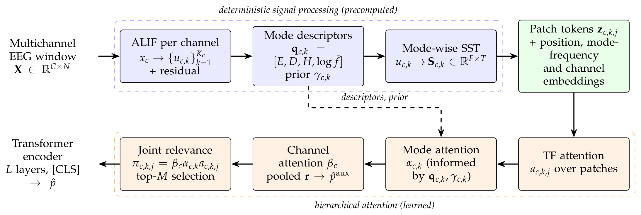
Figure 2.
Original EEG signal and its ALIF decomposition. (a) Band-pass filtered EEG (0.5–40 Hz) of channel F7–T7 around a seizure of recording chb01_03, with the annotated seizure (2996–3036 s, red) and the analysed 5-s window (3006–3011 s, blue). (b) Analysed window with its reconstruction from the modes and the residual (dashed), intrinsic mode functions ordered from fine to coarse time scale with their mean instantaneous frequency, and residual.
Figure 2.
Original EEG signal and its ALIF decomposition. (a) Band-pass filtered EEG (0.5–40 Hz) of channel F7–T7 around a seizure of recording chb01_03, with the annotated seizure (2996–3036 s, red) and the analysed 5-s window (3006–3011 s, blue). (b) Analysed window with its reconstruction from the modes and the residual (dashed), intrinsic mode functions ordered from fine to coarse time scale with their mean instantaneous frequency, and residual.
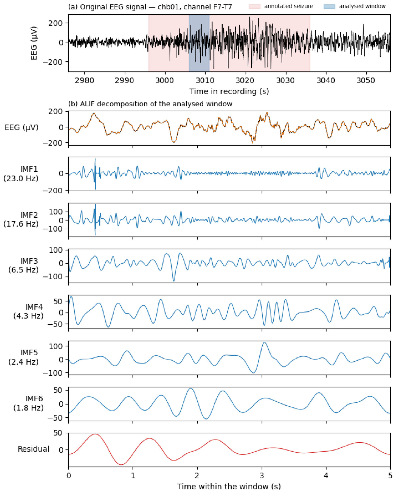
Figure 3.
Direct and mode-wise SST of the analysed window of Figure 2b. (a) SST of the recorded signal. (b) SST of each ALIF mode, labelled with its mean instantaneous frequency. All maps use a logarithmic frequency axis between 0.5 and 40 Hz and compression. The mode-wise maps separate oscillations that interfere in the direct representation.
Figure 3.
Direct and mode-wise SST of the analysed window of Figure 2b. (a) SST of the recorded signal. (b) SST of each ALIF mode, labelled with its mean instantaneous frequency. All maps use a logarithmic frequency axis between 0.5 and 40 Hz and compression. The mode-wise maps separate oscillations that interfere in the direct representation.
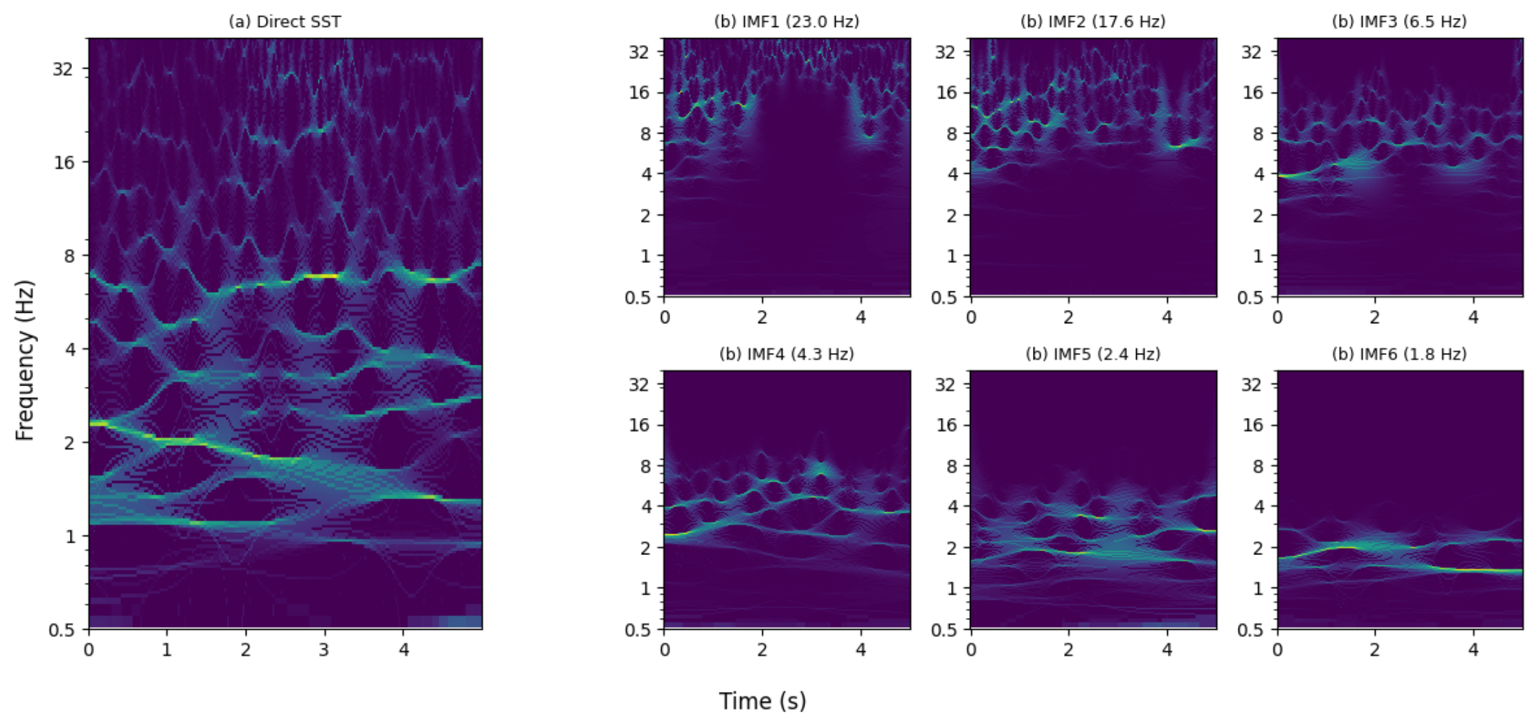
Figure 4.
Effect of the decomposition method (values of Table 8). (a) F1-score versus Rényi entropy of the mode-wise maps (lower entropy means more concentrated maps; dashed line: least-squares fit). (b) F1-score versus decomposition time per 18-channel window (log scale). Squares: non-adaptive decompositions; circles: adaptive decompositions; red: ALIF.
Figure 4.
Effect of the decomposition method (values of Table 8). (a) F1-score versus Rényi entropy of the mode-wise maps (lower entropy means more concentrated maps; dashed line: least-squares fit). (b) F1-score versus decomposition time per 18-channel window (log scale). Squares: non-adaptive decompositions; circles: adaptive decompositions; red: ALIF.
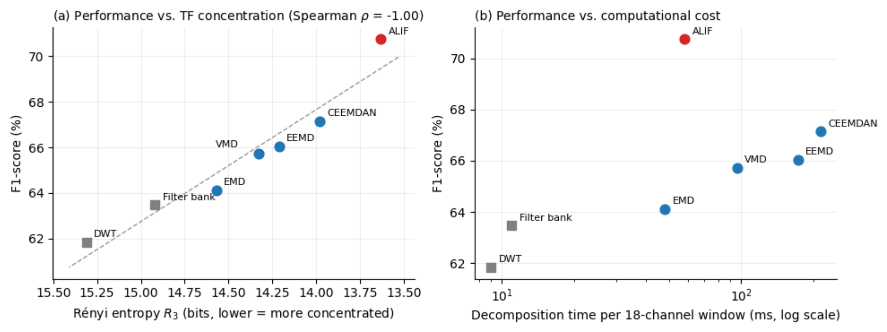
Figure 5.
Robustness of AMST-Former (values of Table 13 and Table 14). (a) F1-score with reduced montages: random subsets (mean ± SD over ten draws) and subsets of the channels with the highest mean relevance , with the corresponding gain. (b) F1-score under white and pink additive noise as a function of the input SNR.
Figure 5.
Robustness of AMST-Former (values of Table 13 and Table 14). (a) F1-score with reduced montages: random subsets (mean ± SD over ten draws) and subsets of the channels with the highest mean relevance , with the corresponding gain. (b) F1-score under white and pink additive noise as a function of the input SNR.
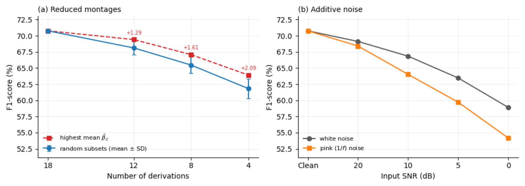
Table 1.
Design choices of representative seizure detection methods and of the proposed AMST-Former. SE: squeeze-and-excitation; FSST: Fourier-based SST; sCSP: sparse common spatial patterns.
Table 1.
Design choices of representative seizure detection methods and of the proposed AMST-Former. SE: squeeze-and-excitation; FSST: Fourier-based SST; sCSP: sparse common spatial patterns.
| Study | Decomposition | TF representation | Learning model | Attention / global modelling | Representation strategy |
|---|---|---|---|---|---|
| Cura and Akan [20] | None | SST | Classical ML | None | Handcrafted features from SST maps |
| Ozdemir et al. [21] | None | FSST | CNN | Local (convolutional) | SST images of the recorded EEG |
| Amiri et al. [22] | None | Adaptive FSST | Linear classifier | sCSP channel selection | TF features of selected channels |
| Zeng et al. [24] | ALIF | None | CNN–LSTM | SE channel attention | One-dimensional IMFs |
| Li et al. [29] | None | STFT | CNN + Transformer | Self-attention | Joint local/global features |
| Lian and Xu [30] | None | None | Graph Transformer | Graph self-attention | Inter-channel dependencies |
| Peng et al. [31] | Wavelet bands | Wavelet | Multi-branch Transformer | Self-attention + distillation | Raw and multiscale branches |
| AMST-Former | ALIF | Mode-wise SST | Transformer | TF, mode and channel attention | Mode-preserving TF tokens |
Table 2.
Implementation settings of AMST-Former.
| Stage | Parameter | Value |
|---|---|---|
| ALIF | Max. number of modes | 6 |
| Filter-length factor ; stopping threshold ; | 1.6; ; 200 | |
| SST | Wavelet; frequency range; | GMW (); 0.5–40 Hz; |
| Tokens | Patch size ; embedding dim. d | ; 128 |
| Retained tokens M | 512 | |
| Encoder | Layers L; heads H; FFN dim.; dropout | 4; 4; 256; 0.1 |
| Training | Optimizer; learning rate; weight decay | AdamW [70]; ; 0.05 |
| Batch size; max. epochs; early-stopping patience | 64; 100; 15 (validation AUPRC) | |
| ; channel dropout (training only) | 0.3; 0.1 |
Table 3.
Third-order Rényi entropy (bits; lower is more concentrated) of three TF representations, 0.5–40 Hz (mean ± SD over 220 ictal and 220 non-ictal CHB-MIT windows).
Table 3.
Third-order Rényi entropy (bits; lower is more concentrated) of three TF representations, 0.5–40 Hz (mean ± SD over 220 ictal and 220 non-ictal CHB-MIT windows).
| Representation | Ictal windows | Non-ictal windows |
|---|---|---|
| CWT scalogram | 16.92 ± 0.16 | 16.87 ± 0.30 |
| Direct SST | 14.85 ± 0.29 | 14.74 ± 0.63 |
| Mode-wise SST (ALIF) | 13.63 ± 0.75 | 13.51 ± 0.65 |
Table 4.
Patient-independent seizure detection on CHB-MIT: published results (taken from the original articles) and AMST-Former. Protocols, class ratios and scoring levels differ; see text. Only metrics that do not depend on the proportion of seizures (sensitivity, specificity, AUC) are reported, since precision, F1-score and AUPRC are not comparable across different class ratios. LOPO: leave-one-patient-out; LOSO: leave-one-subject-out; FA: false alarms; –: not reported.
Table 4.
Patient-independent seizure detection on CHB-MIT: published results (taken from the original articles) and AMST-Former. Protocols, class ratios and scoring levels differ; see text. Only metrics that do not depend on the proportion of seizures (sensitivity, specificity, AUC) are reported, since precision, F1-score and AUPRC are not comparable across different class ratios. LOPO: leave-one-patient-out; LOSO: leave-one-subject-out; FA: false alarms; –: not reported.
| Study | Method | Protocol and scoring | Sens. (%) | Spec. (%) | AUC | False alarms |
|---|---|---|---|---|---|---|
| Ali et al. [67] | Handcrafted features + random forest, 22 channels | Subject-wise 5-fold (and LOSO); event level, continuous EEG | 72.63‡ | – | – | – |
| Farooq et al. [68] | -VAE latent + handcrafted features, boosted trees | LOPO, 24 cases; window level, continuous EEG | 55.05 | 99.67 | 0.950 | 4.72/h |
| Rehman and Mun [69] | 27 handcrafted features, gradient-boosted ensembles | LOSO, 6 seizure-positive patients; event level | 95 | – | ≥0.99 | 0/24 h |
| AMST-Former | ALIF + mode-wise SST + hierarchical Transformer | Repeated subject-wise 5-fold, 22 subjects; window level (1:5) | 97.89 | 84.70 | 0.967 | 1/24 h† |
† Event-level evaluation on continuous recordings (Table 10). ‡ 75.34% under LOSO.
Table 5.
Results of closely related methods evaluated with patient-specific or segment-level protocols (for context only; not comparable with Table 4).
Table 5.
Results of closely related methods evaluated with patient-specific or segment-level protocols (for context only; not comparable with Table 4).
| Study | Method | Dataset | Validation | Reported performance |
|---|---|---|---|---|
| Cura and Akan [20] | SST features + classical ML | CHB-MIT | Segment-level (10-fold) | Acc. 95.13% |
| Ozdemir et al. [21] | FSST images + CNN | CHB-MIT | Patient-specific and leave-one-out variants | Segment-based acc. >99% |
| Amiri et al. [22] | sCSP + adaptive FSST + linear classifier | CHB-MIT | Segment-level (10-fold) | Acc. 98.81%, sens. 98.44%, spec. 99.19% |
| Zeng et al. [24] | ALIF + SE-CNN–LSTM | Bonn and a second database | 10-fold, segment-level | Acc. 100% (binary tasks) |
| Xiao et al. [32] | Self-supervised attention Transformer | CHB-MIT | Patient-specific and cross-patient | Cross-patient F1: 62–68% |
| AMST-Former | ALIF + mode-wise SST + hierarchical Transformer | CHB-MIT | Repeated patient-independent 5-fold | F1 70.76%, AUPRC 0.870 |
Table 6.
Representation ablation (mean ± SD over 50 evaluations). All configurations use the same Transformer encoder and select the M highest-energy patches instead of hierarchical attention.
Table 6.
Representation ablation (mean ± SD over 50 evaluations). All configurations use the same Transformer encoder and select the M highest-energy patches instead of hierarchical attention.
| ID | Representation fed to the Transformer | F1 (%) | AUPRC |
|---|---|---|---|
| R1 | Raw EEG patches | 58.42 ± 2.31 | 0.721 ± 0.018 |
| R2 | Direct SST of each channel | 64.87 ± 2.04 | 0.801 ± 0.015 |
| R3 | ALIF IMFs as one-dimensional patches (no SST) | 61.53 ± 2.27 | 0.764 ± 0.017 |
| R4 | ALIF → per-mode Hilbert spectrum (Hilbert–Huang type) | 63.12 ± 2.11 | 0.786 ± 0.016 |
| R5 | ALIF → reconstruction from retained modes → single SST | 65.04 ± 1.98 | 0.804 ± 0.014 |
| R6 | ALIF → mode-wise SST | 68.93 ± 1.63 | 0.870 ± 0.012 |
Table 7.
Leave-one-out architecture ablation. : change with respect to the full model; p: Holm-adjusted corrected resampled t-test on F1.
Table 7.
Leave-one-out architecture ablation. : change with respect to the full model; p: Holm-adjusted corrected resampled t-test on F1.
| Configuration | F1 (%) | AUPRC | ΔF1 | p |
|---|---|---|---|---|
| Full AMST-Former | 70.76 | 0.870 | – | – |
| – TF attention (uniform ) | 67.12 | 0.842 | -3.64 | 0.014 |
| – mode attention (uniform ) | 65.48 | 0.829 | -5.28 | 0.006 |
| – descriptor prior ( removed) | 68.21 | 0.851 | -2.55 | 0.031 |
| – channel attention (uniform ) | 66.04 | 0.836 | -4.72 | 0.009 |
| Index-based instead of frequency-anchored mode embedding | 64.37 | 0.818 | -6.39 | 0.004 |
| – relevance embedding (Eq. 20) | 66.91 | 0.841 | -3.85 | 0.017 |
| – auxiliary loss () | 68.74 | 0.856 | -2.02 | 0.048 |
| Random instead of relevance-based token selection | 62.58 | 0.802 | -8.18 | 0.002 |
Table 8.
Effect of the decomposition method on detection performance, TF concentration and decomposition time per 18-channel window.
Table 8.
Effect of the decomposition method on detection performance, TF concentration and decomposition time per 18-channel window.
| Decomposition | F1 (%) | AUPRC | (bits) | Time (ms) |
|---|---|---|---|---|
| Fixed filter bank ( bands) | 63.47 | 0.784 | 14.92 | 11 |
| DWT (5 levels) | 61.83 | 0.768 | 15.31 | 9 |
| EMD [11] | 64.12 | 0.792 | 14.57 | 48 |
| EEMD [12] | 66.04 | 0.812 | 14.21 | 173 |
| CEEMDAN [13] | 67.15 | 0.824 | 13.98 | 214 |
| VMD [36] | 65.72 | 0.806 | 14.33 | 96 |
| ALIF (proposed) | 70.76 | 0.870 | 13.63 | 58 |
Table 9.
F1-score (%) of four classifier families trained on direct SST and on mode-wise SST.
| Classifier | Direct SST | Mode-wise SST | p |
|---|---|---|---|
| SVM (RBF kernel) | 64.12 | 67.85 | 0.018 |
| Random forest | 62.47 | 65.93 | 0.024 |
| CNN | 66.31 | 69.42 | 0.011 |
| Vision Transformer | 67.58 | 71.03 | 0.007 |
Table 11.
Sensitivity to the main hyperparameters (validation F1, one parameter varied at a time).
| Parameter | Values tested | Selected | F1 range (%) |
|---|---|---|---|
| Maximum number of ALIF modes | 4, 6, 8, 10 | 6 | 68.9–71.1 |
| Patch size | , , | 69.2–71.0 | |
| Retained tokens M | 128, 256, 512, 1024 | 512 | 68.4–71.3 |
| Embedding dimension d | 64, 128, 256 | 128 | 69.1–70.8 |
| Attention heads H | 2, 4, 8 | 4 | 69.0–70.9 |
| Encoder layers L | 2, 4, 6 | 4 | 68.7–70.6 |
| Auxiliary weight | 0, 0.1, 0.3, 1 | 0.3 | 69.0–70.7 |
Table 13.
F1-score (%) with reduced montages (random subsets: mean ± SD over ten draws).
| Model | 18 ch. | 12 ch. | 8 ch. | 4 ch. |
|---|---|---|---|---|
| AMST-Former (random) | 70.76 | 68.12 ± 1.04 | 65.47 ± 1.28 | 61.83 ± 1.51 |
| AMST-Former (highest ) | 70.76 | 69.41 | 67.08 | 63.92 |
Table 14.
F1-score (%) under additive noise at decreasing input SNR (models not retrained).
| Noise | Model | Clean | 20 dB | 10 dB | 5 dB | 0 dB |
|---|---|---|---|---|---|---|
| White | AMST-Former | 70.76 | 69.12 | 66.84 | 63.47 | 58.91 |
| Pink | AMST-Former | 70.76 | 68.41 | 64.03 | 59.72 | 54.18 |
Table 15.
Deletion analysis on correctly detected ictal windows: area under the curve of versus fraction of deleted tokens (lower means a more faithful ranking).
Table 15.
Deletion analysis on correctly detected ictal windows: area under the curve of versus fraction of deleted tokens (lower means a more faithful ranking).
| Token ranking | Area under deletion curve |
|---|---|
| Random order | 0.412 ± 0.027 |
| Integrated gradients [47] | 0.351 ± 0.022 |
| Hierarchical relevance (Eq. 19) | 0.289 ± 0.018 |
Table 16.
Computational cost per 5-s, 18-channel window (CPU for ALIF and SST; single GPU for the network; batch size 1).
Table 16.
Computational cost per 5-s, 18-channel window (CPU for ALIF and SST; single GPU for the network; batch size 1).
| Model | Params (M) | Front end (ms) | Network (ms) | GPU mem. (MB) |
|---|---|---|---|---|
| AMST-Former, all tokens | 8.7 | 118 | 142 | 812 |
| AMST-Former, top-M tokens | 8.7 | 118 | 49 | 327 |
Disclaimer/Publisher’s Note: The statements, opinions and data contained in all publications are solely those of the individual author(s) and contributor(s) and not of MDPI and/or the editor(s). MDPI and/or the editor(s) disclaim responsibility for any injury to people or property resulting from any ideas, methods, instructions or products referred to in the content. |
© 2026 by the authors. Licensee MDPI, Basel, Switzerland. This article is an open access article distributed under the terms and conditions of the Creative Commons Attribution (CC BY) license (http://creativecommons.org/licenses/by/4.0/).
Copyright: This open access article is published under a Creative Commons CC BY 4.0 license, which permit the free download, distribution, and reuse, provided that the author and preprint are cited in any reuse.