

Submitted:
10 October 2026
Posted:
12 October 2026
You are already at the latest version
Abstract
We study how radial gradient clipping affects the period-two orbit created by a supercritical flip bifurcation near a nondegenerate minimum with a simple maximal Hessian eigenvalue. Clipping leaves the local flip threshold unchanged. For a small clipping threshold \(c\), the stable smooth two-cycle first reaches the clipping boundary at a parameter distance \(Kc^2 + O(c^4)\) from the flip, with an explicit coefficient determined by the potential and the clipping norm. The two cycle points have opposite gradients and therefore reach the boundary simultaneously. A clipped two-cycle cannot have one point strictly inside the smooth region and the other strictly inside the clipped region. Every two-cycle with both points strictly clipped has an exact unit Floquet multiplier and is nonhyperbolic. A solvable planar model illustrates the transition from a stable smooth two-cycle to a neutral family of clipped two-cycles.
Keywords:
gradient maps
; gradient clipping bifurcation
; period-doubling bifurcation
; piecewise-smooth dynamical systems
; switching hypersurfaces
; border collision
; periodic orbits
1. Introduction
Finite-step gradient descent, , is a discrete dynamical system whose behavior near the boundary of linear stability can differ from its gradient-flow approximation [1,2,3,4]. At a nondegenerate local minimum with a simple maximal Hessian eigenvalue , the first stability threshold is . The corresponding multiplier reaches , and a nondegenerate supercritical flip creates a stable period-two branch [5,6,7]. Such oscillations are relevant to the edge-of-stability phenomenon [8]. Recent analyses describe their nonlinear stability and amplitude through higher derivatives and coupling between Hessian eigendirections [9,10,11].
Gradient clipping controls large updates in optimization [12,13,14,15]. We study radial clipping in a norm :
with . Its switching boundary is generated by the same potential as the smooth dynamics. For each fixed , clipping is inactive near a critical point. It therefore preserves the local flip, but can change the newborn oscillation once its amplitude reaches . We ask when this first contact occurs and what restrictions radial clipping imposes on subsequent two-cycles.
1.1. Main Results and Their Relation to Existing Theory
Under the hypotheses in Section 2, we establish three connected results. First, the clipped and smooth maps have identical local germs at the minimum, and the stable smooth two-cycle has leading amplitude , where and is the explicit third- and fourth-derivative expression in (2.22). Second, its first clipping contact satisfies
The two cycle points have exactly opposite gradients and hence reach the boundary simultaneously. Together with the smooth signed square-root parametrization, this balance removes the term of order from the gradient exposure and yields the even-power remainder in (1.1). Third, radial clipping excludes strict smooth–clipped two-cycle itineraries, and every strictly fully clipped two-cycle has an exact unit Floquet multiplier. Thus any continuation into that regime is nonhyperbolic; its existence and nonlinear stability require additional information. A solvable planar model realizes a neutral family of clipped two-cycles after contact.
Smooth flip theory supplies the local birth mechanism [5,6,16,17]; general dynamical-systems background is given in [18,19,20]. Piecewise-smooth and border-collision theory supplies the broader switching framework [21,22,23,24,25,26,27]. Related treatments of discontinuous and nonsmooth dynamics provide further context for switching systems [28,29,30,31]. In particular, quadratic tangency between period-doubling and border-collision loci is already known [32,33,34,35,36]. Our contribution is the explicit coefficient for the endogenous gradient boundary, the improved remainder, and the exact algebraic and spectral rigidity imposed by radial clipping. We retain the smooth derivation to fix conventions and identify the coefficient entering the contact law.
1.2. Organization
2. Setting, Hypotheses and Local Stability
Throughout the paper, and denote the standard Euclidean inner product and norm on , respectively. All gradients, Hessians, and spectral quantities are understood with respect to this Euclidean structure.
Let be an open set and let
be a smooth potential. For a step size , the associated gradient-descent map is
Our aim is to study how a smooth flip bifurcation of (2.1) interacts with the switching boundary generated intrinsically by gradient clipping.
2.1. Clipped Gradient Maps
Let be a norm on . For a clipping threshold , define
Equivalently,
with the convention .
The clipped gradient map is
The maps take values in ; U need not be forward invariant. All orbit statements concern iterates that remain in U. Under (H2) and (H5), the sufficiently small positive levels of near are hypersurfaces: the Hessian is invertible there, and the norm derivative at a nonzero vector is nonzero by Euler’s identity. No global regularity of remote components of is asserted.
The standard Euclidean gradient-clipping rule corresponds to
Associated with (2.3) is the endogenous switching hypersurface
It separates the local phase space into the smooth region
and the clipped region
Accordingly,
whereas in ,
Thus is continuous and piecewise smooth, while its switching geometry is not prescribed independently of the dynamics: the boundary is generated by the same potential V that defines the gradient map.
2.2. The Distinguished Critical Point
We focus on the dynamics near an isolated nondegenerate local minimum of V.
Set
Since H is symmetric, choose an orthonormal eigenbasis satisfying
We denote the maximal eigenvalue and its corresponding unit eigenvector by
The linearization of the smooth gradient map at is
and hence its multipliers are
The distinguished step size at which the maximal-curvature multiplier reaches is
At ,
The parameter
will be used as the local bifurcation parameter throughout the paper.
2.3. Higher-Order Tensors and the Flip Coefficient
We write
viewed as symmetric multilinear forms.
For , let
denote the Euclidean Riesz representative of the linear functional ; namely,
Similarly, denotes the vector determined by for every z. Thus parentheses denote vector contractions, while brackets denote scalar multilinear evaluations.
Define
and
The nonlinear quantity governing the local flip bifurcation is
Equivalently, using the eigenbasis (2.10),
With the flip-normal-form convention used in this paper, define
Thus corresponds to the supercritical case in which a stable small-amplitude period-two branch is created for .
The expression (2.23) is the multivariate gradient-map form of the nonlinear flip criterion: the cubic coupling of the critical direction to all Hessian eigendirections contributes to the sign of the bifurcation coefficient, rather than only the derivatives taken purely along .
2.4. Standing Hypotheses
The following assumptions are imposed unless stated otherwise.
- Regularity. The potential satisfies
- Nondegenerate strict local minimum. The distinguished point satisfies
- Simple maximal curvature. The largest Hessian eigenvalue is simple:
- Supercritical flip nondegeneracy. The coefficient defined in (2.22) satisfiesor equivalently
- Smooth clipping geometry. The clipping norm is of class on .
2.5. Immediate Spectral Consequences
Assumptions (H2)–(H3) imply that the spectral hypotheses required for a simple codimension-one flip bifurcation are automatic for the gradient map.
Indeed, for ,
and therefore, at ,
Hence is the unique multiplier of on the unit circle.
Moreover,
so that
Thus the critical multiplier crosses transversally as passes through .
Thus, under the spectral assumptions (H2)–(H3), the sign of provides the remaining nonlinear nondegeneracy condition that distinguishes the supercritical and subcritical flip cases.
2.6. Local Identity and Fixed Points
Proposition
(Fixed-point invariance). For , .
Proof.
Radial clipping vanishes precisely when its argument vanishes; therefore is equivalent to . □
Theorem
(Local identity and stability). For each fixed there is a radius , independent of η, such that
Under(H1)–(H3), is locally asymptotically stable for and unstable for . At , its only unit-circle multiplier is the simple .
Proof.
Choose with and put , where uses the Euclidean norm in the domain and the clipping norm in the range. The integral formula for the gradient gives . Hence ensures that clipping is inactive, proving the local identity. The multipliers are : all have modulus less than one below , whereas above it. Simplicity of gives the assertion at the threshold. Linearization alone does not determine stability at . □
Corollary
(Local normal-form invariance). The local jets, center-manifold equations and smooth flip coefficients of and coincide. In particular, ℓ is independent of c.
Proof.
The maps agree on an open neighborhood of , so their derivatives and local invariance equations agree. A sufficiently small center manifold of the smooth map gives a common choice; uniqueness of center manifolds is not required. □
The identity also gives equality of local stable sets defined by orbits that remain in this neighborhood, and, when the maps are local diffeomorphisms, equality of unstable-manifold germs. The radius is as : local clipping independence does not supply a uniform neighborhood in this limit. Positive definiteness of H excludes minimizer manifolds and additional center directions; multiple critical eigenvalues and degenerate flip coefficients are outside the present scope.
3. Smooth Flip Bifurcation and the Emerging Period-Two Branch
In this section we study the smooth gradient map
near the critical step size
The local mechanism considered here is the classical simple flip bifurcation of a smooth discrete map [5,6]. For gradient-descent dynamics, Mulayoff and Stich [9] recently derived a multivariate nonlinear stability criterion involving the second-, third-, and fourth-order derivatives of the potential, while Gan [10] formulated edge-of-stability dynamics in a systematic bifurcation-theoretic framework.
Accordingly, the existence of a smooth period-two branch is not the new contribution of the present paper. We reproduce the local reduction because its explicit coefficient enters the switching-separation law derived later; we therefore give a self-contained center-manifold and normal-form derivation in the notation of the present paper.
By the local identity theorem in Section 2, the resulting local bifurcation structure is inherited exactly by the clipped map as long as the bifurcating orbit remains inside the smooth region .
Throughout this section we write
Thus the bifurcation point corresponds to .
Under (H2)–(H3), the multiplier associated with is
whereas all remaining multipliers lie strictly inside the unit disk at .
The nonlinear character of the bifurcation is governed by the coefficient
defined in (2.24). Assumption (H4) gives
which corresponds to the supercritical case.
3.1. Parameter-Dependent Center Reduction
Translate the critical point to the origin, , and define
Then for every sufficiently small , and at ,
whose unique critical multiplier is with eigenvector ; the complementary spectrum lies strictly inside the unit disk.
To incorporate the bifurcation parameter, consider the extended map
Its two-dimensional local center manifold is associated with the critical state direction and the neutral parameter direction, and after restricting to a sufficiently small neighborhood can be represented as
with
The dynamics on the center manifold are described by the scalar map
3.2. Flip Normal Form
We next record the local normal form required for the asymptotic analysis.
Proposition
(Reduced flip normal form). Assume(H1)–(H4). There exists a local near-identity state coordinate, preserving and leaving the physical parameter unchanged, in which the reduced map (3.8) takes the form
where
as .
The cubic coefficient is
or equivalently
Proof.
The critical multiplier is simple and crosses the unit circle transversally (Section 2.5), so the standard parameter-dependent center-manifold and flip-normal-form reductions apply; see [5,37,38]. The linear parameter coefficient is by (3.2), and the quadratic term is eliminated by the standard near-identity transformation for a simple flip; the remaining cubic coefficient is the first flip coefficient.
For the gradient map
one has
Writing , , and , the standard flip coefficient is
Here the left and right critical eigenvectors coincide because J is symmetric, and is invertible. Substitution gives
Using
and the definition of in (2.22) yields
The remainder estimate (3.10) follows from the regularity in (H1) and the parameter-dependent near-identity normal-form transformation. The Taylor remainders also satisfy and for the second iterate below. □
3.3. The Second Iterate
The bifurcating period-two orbit is most conveniently obtained from the fixed points of the second iterate.
Lemma
(Expansion of the second iterate). Under the hypotheses of Proposition 3.1,
where
Proof.
Write
Then
Ignoring terms of order contained in (3.16), one obtains
Since
and
we obtain
The stated remainder estimate follows by substituting (3.10) into the composition. □
Equation (3.15) exhibits explicitly the balance responsible for the square-root amplitude law:
3.4. Existence and Amplitude of the Period-Two Branch
We now obtain the local period-two branch together with its leading amplitude.
Theorem
(Supercritical period-two branch). Assume(H1)–(H4). There exists such that for every
the smooth gradient map possesses a unique local period-two cycle
in a sufficiently small neighborhood of .
The two points satisfy
where
and therefore
The labeling may be chosen so that
Proof.
We first work in the reduced coordinate z.
Set
and seek nonzero solutions of
in the form
By Lemma 3.2,
Define the rescaled bifurcation equation
Under (H1) the rescaled map extends as a function to : since , the gradient map is smooth, and the parameter-dependent flip reduction can be chosen with the finite regularity needed here. Thus the reduced map and the numerator in (3.24) are therefore in and vanishes to third order in , so dividing by yields a function. We set
Since , the nonzero zeros of are
Furthermore,
The implicit function theorem therefore yields two branches
Consequently,
The fixed point is locally the only fixed point of near the origin. Indeed,
so the implicit function theorem excludes nearby nonzero period-one fixed points. Hence the two nonzero solutions of
have prime period two.
After the normal-form state change, the physical embedding is , where . Thus
Since
and
we have
Therefore
which proves (3.19).
Finally, the two nonzero points form a single two-cycle, so after possibly interchanging the labels we obtain (3.22).
For completeness, these branches exhaust the nearby nonzero roots. Divide the second-iterate equation by z and extend smoothly at zero. Its derivative in at the origin is , so it determines , where . The function is strictly convex near zero and has its unique minimum there; hence each sufficiently small positive has exactly two nonzero roots. Every sufficiently small periodic orbit is a full local orbit and belongs to the chosen center manifold. Thus the two roots exhaust the local two-cycle. The direct reduction in Section 4.3 independently gives the same local uniqueness without choosing a center manifold. □
3.5. Stability of the Emerging Cycle
We next verify the local stability of the branch.
Theorem
(Stability of the supercritical period-two cycle). Under(H1)–(H4), the period-two cycle given by Theorem 3.3 is locally asymptotically stable for all sufficiently small .
Along the critical center direction, the multiplier of the two-step map satisfies
Proof.
Differentiate the expansion (3.15):
At either point , Theorem 3.3 gives
Hence
Thus the center multiplier lies strictly inside the unit disk for all sufficiently small .
At , every transverse multiplier of the two-step map equals
and by (2.28),
Therefore
By continuity, all transverse multipliers remain strictly inside the unit disk along the sufficiently small period-two branch.
The reduction principle then implies local asymptotic stability of the full period-two cycle. □
3.6. Transfer to the Clipped Map Before Switching
We finally transfer the preceding smooth bifurcation result to the clipped map.
Corollary
(Pre-contact period-two cycle for the clipped map). Assume(H1)–(H5)and fix . Then there exists
such that for every
the clipped map
possesses the same locally asymptotically stable period-two cycle as the smooth gradient map .
Moreover,
Proof.
For the fixed value , let be given by Theorem 2.2. By Theorem 3.3,
Hence there exists such that
for every .
On this ball,
by Theorem 2.2. Therefore the two maps have exactly the same period-two cycle and the same local derivatives along that cycle. Its local asymptotic stability follows from Theorem 3.4. □
4. Switching Geometry and the Separation Law
We now study how the smooth period-two branch constructed in Section 3 approaches the endogenous switching hypersurface
A key structural feature of gradient maps appears at this point. For an arbitrary period-two cycle of gradient descent, the gradients at its two points are exactly opposite. Consequently, their gradient norms are identical for every norm .
This identity has two important consequences.
First, the two points of the smooth period-two orbit necessarily reach the clipping boundary simultaneously. Thus, unlike a generic piecewise-smooth map, the present gradient-generated switching problem does not exhibit a splitting of the two first-contact parameters.
Second, the common gradient magnitude along the bifurcating cycle has a particularly simple expansion in the square-root parameter . This structure will yield the quadratic separation law in Section 4.
4.1. Exact Gradient Balance on a Period-Two Cycle
We begin with an exact identity that does not rely on the local bifurcation expansion. An equivalent balance relation appears in the recent characterization of gradient-descent period-two orbits by Litman [11]. Since this identity is the starting point of the switching analysis below, we include its elementary proof for completeness.
Proposition
(Exact gradient balance). Let , and suppose that is a period-two cycle of the smooth gradient map
that is,
Then
In particular,
Consequently, for every norm ,
Proof.
The first identity in (4.1) gives
and hence
Similarly,
implies
This proves (4.2) and (4.3).
Since every norm is even,
and therefore
□
4.2. Midpoint and Half-Difference Coordinates
For the bifurcating period-two cycle
define its midpoint and half-difference by
Thus
Theorem 3.3 implies
The period-two equations yield considerably more structure.
Lemma
(Midpoint–difference equations). For every smooth period-two cycle of written in the form (4.7),
Proof.
By Proposition 4.1,
and
Adding and subtracting these identities gives (4.9) and (). □
4.3. Square-Root Parametrization and Parity
The following direct reduction justifies both the regularity and the parity; exchanging the two points alone would not establish smoothness in the signed square-root parameter.
The implicit function theorem applied to (4.9), whose midpoint derivative at the origin is , gives a unique smooth even function , with
Insert this function into the difference equation and denote its left-hand side minus by . This residual is odd in d. Write , . The perpendicular equation has derivative in w at the origin, which is invertible by (H3). It therefore determines uniquely ; this function is odd in t, and , so with smooth W. In dimension one this perpendicular equation is absent.
Dividing the remaining scalar equation by and extending smoothly to gives, with ,
Here the cubic contribution is . The derivative in at is . Hence the scalar equation determines with . Its inverse satisfies . Every sufficiently small nontrivial cycle is captured by this reduction, since the perpendicular solution at is zero. This also proves local uniqueness of the unordered cycle.
Set , using the positive smooth extension with value for the quotient at zero. Then t and d are smooth and odd, and is smooth and even.
Introduce the signed square-root parameter
The two-cycle equations are invariant under the transformation
which merely exchanges the two points of the cycle.
The construction above gives a parametrization with
Hence the midpoint is even and the half-difference is odd in .
Proposition
(Refined two-cycle expansion). Assume(H1)–(H4). The period-two branch can be parametrized by the signed variable ε, with , such that
where
Consequently,
Proof.
The parity relations (4.12) imply that the local expansions have the form
and
By Theorem 3.3,
It remains to determine . Taylor expansion of the gradient about gives
Apply (4.17) to and and add the resulting expressions. Using (4.9), we obtain
Here we used
and the cancellation of all terms odd in d.
Substituting
and
into (4.18) gives
Since H is invertible,
This proves (4.15) and hence (4.16). □
4.4. A Consistency Derivation of the Flip Amplitude
The midpoint–difference equations also provide a direct, coordinate-free derivation of the leading oscillation amplitude.
Proposition
(Amplitude identity). Under(H1)–(H4), the leading amplitude satisfies
Equivalently,
in agreement with (3.21).
Proof.
Expand the difference equation () to cubic order.
Using
Taylor expansion gives
On the other hand,
Take the Euclidean inner product of () with and compare the coefficients of .
The unknown correction in d cancels because
Thus,
Since
and
equation (4.22) becomes
Dividing by and rearranging gives
By definition of ,
□
4.5. Gradient Exposure Along the Bifurcating Cycle
Define the common gradient exposure of the smooth period-two cycle by
The equality is exact by Proposition 4.1.
Using the half-difference coordinate, one obtains the exact formula
This identity is considerably stronger than a direct Taylor expansion of at the two cycle points.
Theorem
(Asymptotic switching geometry of the two-cycle). Assume(H1)–(H5). As ,
where
Equivalently,
In particular, there is no term of order μ in (4.25).
Proof.
Set
By Proposition 4.1,
Using positive homogeneity of the norm,
Furthermore,
Substituting (4.28) and (4.29) into (4.24) yields
Since ,
where
Finally, using
gives
□
4.6. Simultaneous First Contact
We now record the most important geometric consequence of the exact gradient balance.
Theorem
(Simultaneous switching contact). Let be the smooth period-two branch from Theorem 3.3. For every sufficiently small ,
Likewise,
Hence the two points of a smooth gradient-descent period-two cycle cannot cross a radial clipping boundary sequentially.
Proof.
By Proposition 4.1,
Each of the three statements follows immediately by comparing this common value with the clipping threshold c. □
Corollary
(No pre-contact splitting of the two-cycle). There do not exist two distinct first-contact parameters
for the two points of the smooth period-two branch. Whenever the first switching contact exists, it is a simultaneous two-point contact.
Proof.
If one point lies on , then the other lies on by Theorem 4.6. □
4.7. Exposure Factorization and Unique Contact
Lemma
(Exposure factorization and monotonicity). For sufficiently small ,
Consequently, E is strictly increasing for small .
Proof.
The odd half-difference has the form with and . By (4.24), take . The norm is smooth at the nonzero vector , so is and . For , near zero, since is bounded below and is bounded. □
Define by and set . These are the unique local first-contact parameters for small .
4.8. Quadratic Separation with an Explicit Coefficient
Theorem
(Flip-to-switching separation law). Under(H1)–(H5), the local first-contact parameter exists and is unique for sufficiently small . As ,
Proof.
Continuity, strict monotonicity and give local existence and uniqueness. At contact the factorization gives . Since , first and then, using , . Thus . Substitute , and . □
In an orthonormal Hessian eigenbasis the coefficient is
For Euclidean clipping , so . The coefficient combines linear curvature, nonlinear saturation, and the clipping norm in the critical direction. At fixed curvature, a larger gives a smaller oscillation and later contact. The exponent two agrees with the generic tangency mechanism [33]; the explicit coefficient, simultaneous contact, and remainder use the gradient structure.
4.9. Dynamical Meaning of the Contact
For both points lie in , so the stable smooth cycle is also a cycle of . At equality both lie on ; the clipping operator still equals the identity there, and the cycle equations remain valid. For within the local interval, the smooth reference branch lies in and generally ceases to be a cycle of the clipped map. These conclusions follow by comparing the strictly increasing exposure with c. At the boundary the map is generally nondifferentiable; smooth-side stability does not assert stability for all perturbations of the boundary cycle. Figure 2 illustrates the geometry and parameter separation.
5. Post-Contact Degeneracy of Clipped Two-Cycles
Section 4 shows that the smooth period-two branch created by the supercritical flip reaches the switching hypersurface simultaneously at both of its points.
The radial clipping structure imposes a further restriction: a genuine period-two orbit cannot have one point in the smooth region and the other in the strictly clipped region. This excludes strict mixed itineraries, but does not assert existence of a continuation or exclude cycles involving boundary points. The results below concern cycles whose two points both lie in .
The post-contact results obtained below are not consequences of the generic border-collision theory cited in Section 1. They rely specifically on the radial structure of the clipping operator.
The purpose of this section is to characterize the universal structure of such fully clipped period-two orbits. The main result is that every fully clipped period-two orbit is necessarily nonhyperbolic: its two-step monodromy matrix has an exact multiplier equal to one.
This neutral multiplier is not a consequence of the local flip normal form. It arises directly from the radial normalization inherent in gradient clipping.
5.1. Fully Clipped Period-Two Orbits
We first record the exact algebraic structure of a fully clipped period-two orbit.
Proposition
(Exact geometry of a fully clipped two-cycle). Let
be a genuine period-two orbit of
and suppose
Then
Moreover, there exist
and numbers
such that
Proof.
The period-two relations are
Therefore
Since both points lie in the strictly clipped region,
Taking norms in (5.7) gives
Define
Then
Because radial clipping preserves direction,
and
Setting
gives the result. □
5.2. Exclusion of Mixed Period-Two Itineraries
We now establish the restriction imposed by radial clipping.
Proposition
(No mixed smooth–clipped period-two orbit). A radial clipped gradient map cannot possess a genuine period-two orbit
such that exactly one point lies in and the other lies in .
More generally, if one point is strictly smooth, the other is strictly smooth as well: their clipped gradient outputs are opposite and have the same norm less than c. Otherwise both points belong to . A boundary–strictly-clipped pair is not excluded by this argument, and a classical two-step derivative need not exist for such a pair.
Proof.
Suppose, for contradiction, that
Then the period-two equations imply
Taking the clipping norm gives
which contradicts
The opposite mixed itinerary is ruled out identically. For the more general assertion, the opposite clipped outputs have equal norm, and . If one output has norm less than c, so does the other, forcing both original gradients to have norm less than c. □
5.3. Differential Structure in the Clipped Region
We now examine the differential structure of the radial clipping operator in the strictly clipped region. This structure will be the key ingredient in the spectral analysis of fully clipped period-two orbits.
Let
For any nonzero vector , write
and define the covector
Since is positively homogeneous of degree one, Euler’s identity gives
Moreover, the derivative of a positively homogeneous function of degree one is homogeneous of degree zero. Hence, since with ,
In the strictly clipped region
the clipping operator takes the form
For any , differentiation yields
Using
and (5.10), we obtain
Equivalently,
The operator
has a simple geometric interpretation. By (5.9),
and
Thus projects onto
the tangent space of the unit -sphere at u, along the radial direction spanned by u.
In particular, multiplying (5.11) from the left by gives
Equation (5.12) expresses the differential degeneracy created by radial clipping: infinitesimal variations in the gradient-magnitude direction are annihilated, whereas only variations tangent to the clipping sphere contribute to the differential of the clipped update.
For every , the chain rule therefore gives
Proposition
(Pointwise neutral covector). Let and set
Then
In particular,
Proof.
Using (5.13),
By (5.12),
Hence the second term vanishes and
Thus is a left eigenvector of associated with the eigenvalue 1. Therefore
□
5.4. Universal Unit Multiplier for Fully Clipped Two-Cycles
We now obtain the principal post-contact result.
Theorem
(Universal unit multiplier).
Let
be any fully clipped period-two orbit of .
Let
be the corresponding two-step monodromy matrix.
Then
More precisely, if u is the common clipping direction defined by Proposition 5.1, then
and
Hence
Proof.
By Proposition 5.1, there exist and a vector u with such that
Since every norm is even,
and therefore
Thus
At , the normalized gradient direction is u. Hence Proposition 5.3 gives
At , the normalized gradient direction is . Applying Proposition 5.3 with gives
Since , this is equivalent to
Consequently,
Thus is a nonzero left eigenvector of associated with the eigenvalue 1. Therefore
□
Corollary
(Fully clipped period-two cycles are nonhyperbolic). Every fully clipped period-two orbit of a radial clipped gradient map is nonhyperbolic.
Proof.
Theorem 5.4 gives a multiplier equal to 1, which lies on the unit circle. □
Corollary
(No linear exponential attraction). A fully clipped period-two orbit cannot be linearly exponentially asymptotically stable.
Proof.
Linear exponential asymptotic stability requires every Floquet multiplier of the period-two orbit to lie strictly inside the unit disk. Theorem 5.4 provides an exact multiplier equal to 1. □
5.5. The Spectral Transition at First Contact
Before contact, the smooth period-two orbit is hyperbolically attracting along its critical direction.
By Theorem 3.4,
At the first switching contact,
Hence
Since
this becomes
Thus the smooth cycle reaches the switching boundary while still weakly attracting:
Any fully clipped period-two orbit beyond contact, however, satisfies
in at least one direction.
This yields the following conclusion.
Corollary
(Loss of hyperbolicity under fully clipped continuation).
Suppose that a period-two orbit admits a continuation from the first switching contact into the fully clipped regime. Then every such fully clipped period-two continuation is necessarily nonhyperbolic.
In the smooth-side limit at contact, the critical multiplier satisfies
and therefore
Thus the smooth-side limiting cycle is still weakly attracting. This statement concerns the smooth reference derivative, not a classical derivative of the clipped map on the boundary. By Theorem 5.4, every fully clipped period-two orbit carries an exact unit multiplier.
5.6. Degeneracy of the Period-Two Continuation Equation
A period-two point of the clipped map is a solution of
If the two-cycle were hyperbolic, one would normally attempt to continue it by applying the implicit function theorem to
The universal unit multiplier prevents this.
Proposition
(Singularity of the post-contact continuation problem). Let y belong to a fully clipped period-two orbit. Then
is singular.
Consequently, assumptions(H1)–(H5)do not yield a standard implicit-function continuation of the period-two branch through the fully clipped regime.
Proof.
By Theorem 5.4,
Hence
so the derivative of the period-two fixed-point equation is singular. □
5.7. Euclidean Clipping
For the Euclidean norm,
the geometry becomes especially transparent.
If
then in the clipped region
Hence
The radial covector satisfies
For a fully clipped period-two orbit with gradient directions ,
Thus the unit multiplier has a direct geometric interpretation: Euclidean clipping removes the derivative of the update in the radial gradient-magnitude direction.
An exact unit multiplier does not alone imply nonlinear instability or a family of cycles. It makes singular, so the standing hypotheses do not guarantee a standard implicit-function continuation after contact. Additional nonlinear information must determine existence and stability. The planar model below supplies one realization. Also, unit eigenvalues of individual Jacobians do not imply a unit multiplier for arbitrary longer orbits: the common covector argument uses the opposite gradient directions of a two-cycle.
6. A Completely Solvable Planar Gradient Model
We now present a two-dimensional model for which the smooth flip bifurcation, the first clipping contact, the separation coefficient, and the post-contact dynamics can all be computed explicitly.
Consider the potential
where
We use the standard Euclidean clipping norm throughout this section.
The gradient is
For convenience, define
The condition implies
and hence
Thus is the unique critical point of V and is a strict global minimum.
6.1. Verification of the Standing Hypotheses
At the origin,
Since
the maximal Hessian eigenvalue is
and its normalized eigenvector is
The flip threshold is therefore
Since the potential is even in x,
Moreover,
Hence
Thus the flip is supercritical.
The first flip coefficient is
The general amplitude formula gives
or
Finally, the general Euclidean separation coefficient becomes
We shall recover all of these quantities below from the exact dynamics.
6.2. Exact Smooth Gradient Dynamics
The ordinary gradient-descent map is
The line
is invariant. On L, the dynamics reduce to the odd scalar map
Because is odd, a symmetric period-two orbit has the form
The condition
is equivalent to
Set
Then
The small-amplitude root is therefore
The positive small root is defined for . The other quadratic root does not tend to zero at the flip; the uniqueness statements in this paper concern the local branch.
Thus the smooth period-two branch is given explicitly by
where
6.3. Exact Verification of the Square-Root Law
Let
Then
Solving (6.21) gives
Taking the square root yields
Hence
with
exactly as predicted by (6.16).
Because the model is reflection-symmetric, the midpoint of the smooth two-cycle remains exactly at the critical point:
6.4. Stability of the Smooth Period-Two Branch
The derivative of the scalar map is
Using the cycle equation (6.21), one obtains
Since is even, the critical multiplier of the two-step map is
For ,
in agreement with Theorem 3.4.
The transverse multiplier is
Since , at one has , so the transverse multiplier stays inside the unit disk. Consequently, the smooth period-two cycle is locally asymptotically stable for all sufficiently small .
6.5. Exact Gradient Exposure
Figure 5 visualizes one-step exchange, the resulting alternation, and convergence to the smooth cycle. The clipped example in that figure illustrates the exact family constructed below.
At the positive point of the cycle,
By the exact period-two relation,
Hence the common Euclidean gradient exposure is
Using (6.30),
In particular,
and therefore
again agreeing with the general separation coefficient (6.17).
6.6. Exact Switching-Contact Equation
The first contact occurs when
Hence at contact
Substituting this into (6.21) gives the exact scalar equation
At
we have
and
Thus the implicit function theorem gives a unique smooth first-contact curve
for sufficiently small c.
6.7. Exact Verification of the Separation Law
Write
Substituting this expansion into (6.45) and comparing powers of c gives
and
Therefore
The leading coefficient
coincides exactly with
as predicted by Theorem 4.9.
This model therefore verifies not only the quadratic exponent but also the absence of a cubic correction.
6.8. The Fully Clipped Symmetric Branch
We now turn to the post-contact regime. Define
and consider the pair
Its gradient magnitude is
and a direct calculation gives
with as in (6.45). Hence at , and since for all sufficiently small c,
sufficiently close to the contact value. Both points therefore lie in the fully clipped region. On the invariant axis, radial clipping acts as
and since ,
Thus:
Proposition
(Explicit fully clipped period-two branch). For every sufficiently small and every sufficiently close to ,
is a fully clipped period-two orbit.
Its amplitude satisfies exactly
6.9. A Continuum of Clipped Period-Two Cycles
The symmetric clipped cycle is not isolated.
For sufficiently small and sufficiently close to contact, we have
By continuity, there exists such that
for every
Define
After reducing if necessary,
Since
radial clipping gives
We therefore obtain the following stronger result.
Theorem
(A local family of clipped period-two cycles). For every sufficiently small and sufficiently close to contact, there exists such that
is a one-parameter family of fully clipped period-two cycles.
Equivalently,
on a nontrivial interval of the positive clipped component and on its image under .
Proof.
For , both points lie in the clipped regime by (6.59).
At , the gradient points in the positive x direction, so the clipped step is exactly
Therefore
At , the gradient points in the negative x direction, so the clipped step is
Thus
□
Remark (Geometric meaning of the unit multiplier)
The continuum in Theorem 6.2 gives a concrete nonlinear interpretation of the universal unit multiplier proved in Theorem 5.4.
The neutral multiplier is not merely an artifact of linearization: in this model the two-step map is exactly the identity along the one-dimensional clipped family.
6.10. Exact Post-Contact Multipliers
Consider the period-two cycle
Set
At either point, the Euclidean clipping direction is parallel to . Therefore
Since
the one-step Jacobians along the clipped cycle are
Hence the two-step monodromy matrix is
Thus the two multipliers are
and
For the symmetric member ,
At the switching contact,
so the outer limiting transverse multiplier becomes
Since
as and
one has
for all sufficiently small c.
By continuity, after reducing the post-contact parameter interval and the family interval , both transverse one-step multipliers have modulus less than one. Hence the local clipped family is transversely attracting while remaining exactly neutral along its one-dimensional period-two direction.
6.11. The Local Transition in the Solvable Model
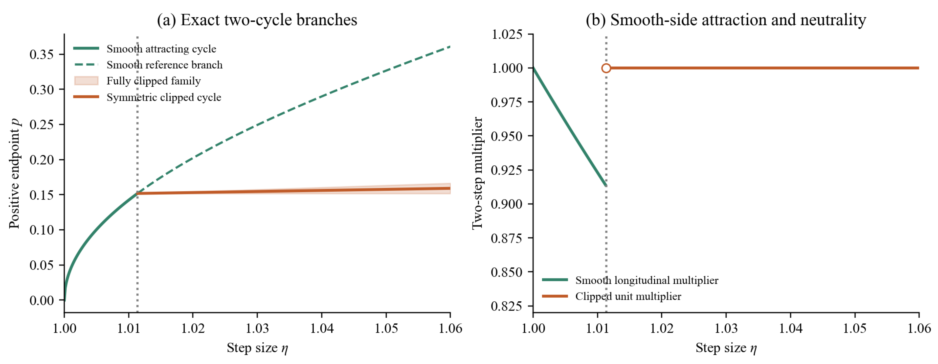
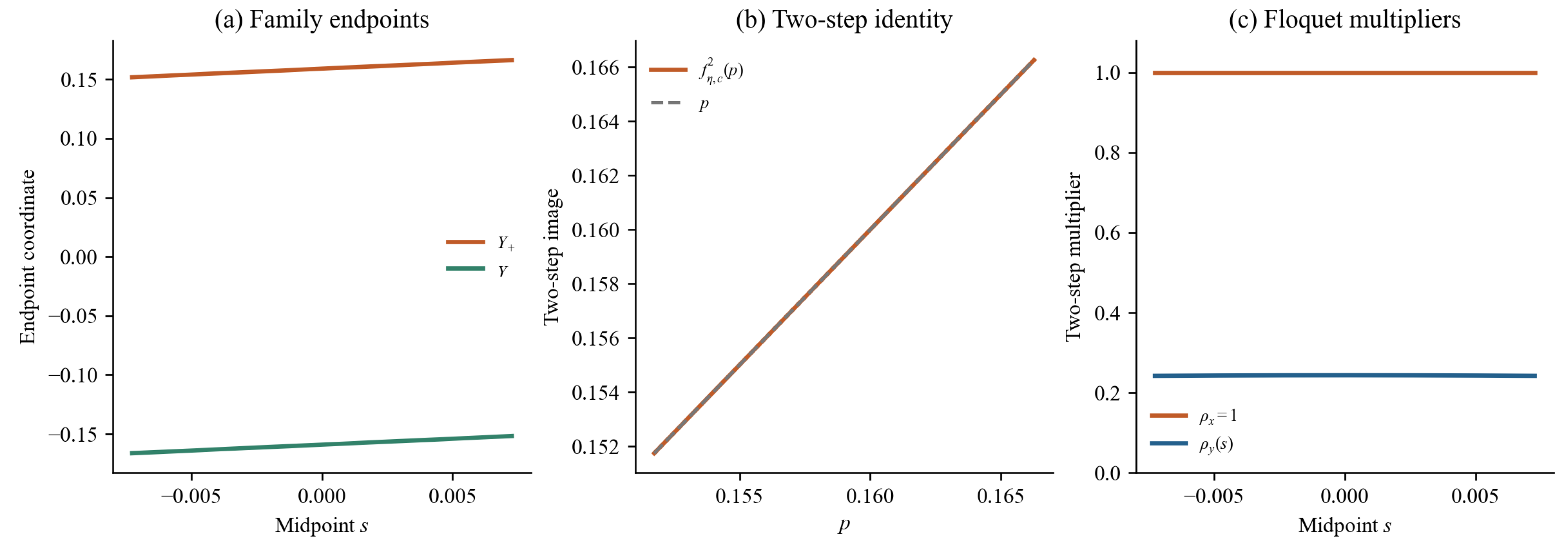
Figure 6 displays the continuum of clipped two-cycles, the identity of the two-step map along this family, and the exact longitudinal and transverse multipliers.
The planar model provides an explicit realization of the entire smooth-to-clipped scenario. For the origin is locally asymptotically stable; for there is a unique small stable smooth two-cycle whose amplitude grows as
At both points reach the clipping boundary simultaneously with
For sufficiently close to contact, the clipped map possesses a one-parameter family of period-two cycles with exact step constraint , and the smooth critical multiplier is replaced by the exact neutral multiplier . The model thus exhibits the transition from a stable smooth period-two branch, through a simultaneous clipping contact, to a neutral family of clipped two-cycles.
6.12. A Concrete Parameter Choice
To make the preceding formulas explicit, consider the parameter choice
Then
and therefore
Hence the smooth period-two branch satisfies , while the first switching threshold obeys
with the next correction computable explicitly:
The example thus provides an explicit realization of the general quadratic separation law of Section 4.
Figure 7.
Exact planar-model formulas for , , and , satisfying . Here r is the small positive root of , and . (a) The smooth symmetric cycle has amplitude . After contact, the shaded open interval parametrizes clipped cycles on the invariant axis; its boundaries are excluded. The solid orange line selects . (b) The smooth longitudinal multiplier remains below one up to contact, while strictly clipped cycles have multiplier one. The open marker excludes a classical clipped derivative at the boundary. Curves are evaluations of analytic formulas, not trajectory simulations.
Figure 7.
Exact planar-model formulas for , , and , satisfying . Here r is the small positive root of , and . (a) The smooth symmetric cycle has amplitude . After contact, the shaded open interval parametrizes clipped cycles on the invariant axis; its boundaries are excluded. The solid orange line selects . (b) The smooth longitudinal multiplier remains below one up to contact, while strictly clipped cycles have multiplier one. The open marker excludes a classical clipped derivative at the boundary. Curves are evaluations of analytic formulas, not trajectory simulations.
7. Conclusion and Discussion
We studied the first interaction between a smooth flip bifurcation and the endogenous switching geometry generated by radial gradient clipping. The mechanism operates on two sharply separated scales: clipping is locally invisible near the critical point and becomes dynamically relevant only at finite amplitude.
7.0.0.1. Local scale.
For every fixed the clipped map coincides with the ordinary gradient map on a neighborhood of a nondegenerate critical point; hence the fixed point, its linearization, its local invariant structures, its center-manifold reduction, and its smooth flip coefficient are independent of the clipping threshold. In particular, for a strict local minimum with simple maximal Hessian eigenvalue , the first stability threshold remains
Under the supercriticality condition
the loss of stability creates a stable smooth period-two branch
7.0.0.2. Finite-amplitude scale.
Clipping becomes active only when this orbit reaches the switching hypersurface
The gradient structure makes the interaction rigid: every smooth period-two orbit satisfies the exact identity
so both points have identical clipping exposure and reach simultaneously. Matching the square-root amplitude scale with the threshold produces the principal asymptotic law
which for Euclidean clipping becomes
The even-power expansion reflects an additional symmetry of the gradient problem: in the signed square-root parameter the half-difference of the two-cycle is odd while its midpoint is even, which together with (7.4) removes the cubic correction from the contact curve.
7.0.0.3. Post-contact scale.
A clipped period-two orbit cannot mix strictly smooth and strictly clipped points. This restriction alone does not guarantee a post-contact continuation or exclude boundary itineraries. Every strictly fully clipped period-two orbit obeys the exact step-length constraint
Most importantly, radial clipping creates an unavoidable neutral direction: the monodromy matrix
of a fully clipped period-two orbit satisfies
Every fully clipped two-cycle is therefore nonhyperbolic: the radial normalization removes first-order information in the gradient-magnitude direction. The solvable planar model of Section 6 shows that this unit multiplier is not a formal artifact — it corresponds to an actual loss of isolation of the periodic orbit.
7.1. Dynamical Interpretation
The results separate two effects that are often conflated. The first is the loss of local stability of the minimum: a smooth gradient-descent phenomenon governed by , , , and unaffected by clipping. The second is the modification of an already finite-amplitude trajectory once it reaches . Clipping does not postpone the first local flip threshold; it introduces a second dynamical scale beyond it, the switching-contact scale . This distinction is useful when interpreting large-step optimization dynamics: linear stability determines when the critical point loses stability, while the clipping threshold determines when the resulting nonlinear oscillation begins to experience a different piecewise-smooth evolution.
7.2. Limitations
The theory focuses on an isolated nondegenerate minimum with a simple maximal Hessian eigenvalue, which isolates a one-dimensional flip mode but excludes the additional neutral directions that arise when the set of minimizers forms a manifold. Second, the post-contact unit multiplier prevents a universal hyperbolic continuation theorem: under the present assumptions alone, the existence, uniqueness, and nonlinear stability of a fully clipped continuation are not determined. Third, the paper treats radial clipping; coordinatewise clipping, adaptive normalization, momentum, and stochastic mini-batch updates generate different switching geometries. Finally, the analysis is local in the bifurcation parameter and does not classify the remote global dynamics after the orbit enters the clipped region.
7.3. Directions for Further Work
Several extensions appear natural: reducing the nonhyperbolic post-contact dynamics to a higher-order scalar or center-manifold normal form, which the exact unit multiplier suggests may form a new class of degenerate border interactions specific to radial gradient maps; replacing the isolated minimum by a Morse–Bott manifold of minima, combining the flip direction with tangent directions; degenerate smooth flips with , where a matching principle , suggests the general contact scale ; and determining which structures persist for momentum, stochastic gradients, and nonradial clipping.
7.4. Final Perspective
Near a nondegenerate minimum, radial gradient clipping is locally invisible: , so the smooth map determines when the first oscillatory instability is born. Once the oscillation reaches finite amplitude, the same potential generates an endogenous switching boundary at the explicit scale
At that point the dynamics cease to be governed solely by the smooth flip normal form: radial clipping removes the gradient-magnitude degree of freedom and forces any strictly fully clipped period-two cycle to carry an exact neutral multiplier. The clipped gradient map thus exhibits a sharp transition from smooth bifurcation theory to intrinsically nonhyperbolic switching dynamics, with the transition scale determined explicitly by the local geometry of the underlying potential.
Author Contributions
Both authors contributed to the conception, analysis, and writing of the manuscript.
Funding
The authors declare that no specific funding was received for this work.
Data Availability Statement
Data sharing is not applicable to this article as no datasets were generated or analysed during the current study.
Acknowledgments
During the preparation of this work, the authors used the DeepSeek V4 Harness (deepseek-v4-flash model) for typesetting, compilation, and manuscript-preparation assistance, and OpenAI ChatGPT (GPT-5.6 Sol) for mathematical discussion, language editing, and manuscript organization. All mathematical arguments, references, and conclusions were independently checked by the authors, who take full responsibility for the manuscript.
Conflicts of Interest
The authors declare that they have no conflict of interest.
References
- Robbins, H.; Monro, S. A Stochastic Approximation Method. Ann. Math. Stat. 1951, 22, 400–407. [Google Scholar] [CrossRef]
- Polyak, B.T. Introduction to Optimization. In Translations Series in Mathematics and Engineering; Optimization Software: New York, 1987. [Google Scholar]
- Nesterov, Y. Lectures on Convex Optimization. In Springer Optimization and Its Applications, 2 ed.; Springer: Cham, 2018; Vol. 137. [Google Scholar]
- Bottou, L.; Curtis, F.E.; Nocedal, J. Optimization Methods for Large-Scale Machine Learning. SIAM Rev. 2018, 60, 223–311. [Google Scholar] [CrossRef]
- Kuznetsov, Y.A. Elements of Applied Bifurcation Theory. In Applied Mathematical Sciences, 3 ed.; Springer: New York, 2004; Vol. 112. [Google Scholar]
- Guckenheimer, J.; Holmes, P. Nonlinear Oscillations, Dynamical Systems, and Bifurcations of Vector Fields. In Applied Mathematical Sciences; Springer: New York, 1983; Vol. 42. [Google Scholar]
- Hale, J.K.; Koçak, H. Dynamics and Bifurcations. In Texts in Applied Mathematics; Springer: New York, 1991; Vol. 3. [Google Scholar]
- Cohen, J.M.; Kaur, S.; Li, Y.; Kolter, J.Z.; Talwalkar, A. Gradient Descent on Neural Networks Typically Occurs at the Edge of Stability. In Proceedings of the International Conference on Learning Representations, 2021. [Google Scholar]
- Mulayoff, R.; Stich, S.U. On the Stability of Nonlinear Dynamics in GD and SGD: Beyond Quadratic Potentials. Proc. Proc. 39th Annu. Conf. Learn. Theory. PMLR, Preliminary version; 2026, arXiv:2602.14789Vol. 336, Proceedings of Machine Learning Research, 5210–5243. [Google Scholar]
- Gan, E. A Bifurcation Theory Framework for Gradient Descent on the Edge of Stability. arXiv 2026, arXiv:2606.15551. [Google Scholar]
- Litman, E. The Origin of Edge of Stability. arXiv 2026, arXiv:2604.20446. [Google Scholar]
- Pascanu, R.; Mikolov, T.; Bengio, Y. On the Difficulty of Training Recurrent Neural Networks. In Proceedings of the Proceedings of the 30th International Conference on Machine Learning, 2013; Proceedings of Machine Learning Research; Vol. 28. [Google Scholar]
- Zhang, J.; He, T.; Sra, S.; Jadbabaie, A. Why Gradient Clipping Accelerates Training: A Theoretical Justification for Adaptivity. In Proceedings of the International Conference on Learning Representations, 2020. [Google Scholar]
- Koloskova, A.; Hendrikx, H.; Stich, S.U. Revisiting Gradient Clipping: Stochastic Bias and Tight Convergence Guarantees. Proc. Proc. 40th Int. Conf. Mach. Learn. PMLR 2023, Vol. 202, 17343–17363. [Google Scholar]
- Goodfellow, I.; Bengio, Y.; Courville, A. Deep Learning; MIT Press: Cambridge, MA, 2016. [Google Scholar]
- Chow, S.N.; Hale, J.K. Methods of Bifurcation Theory. In Grundlehren der mathematischen Wissenschaften; Springer: New York, 1982; Vol. 251. [Google Scholar]
- Wiggins, S. Introduction to Applied Nonlinear Dynamical Systems and Chaos. In Texts in Applied Mathematics, 2 ed.; Springer: New York, 2003; Vol. 2. [Google Scholar]
- Arnold, V.I. Geometrical Methods in the Theory of Ordinary Differential Equations. In Grundlehren der mathematischen Wissenschaften; Springer: New York, 1983; Vol. 250. [Google Scholar]
- Sotomayor, J. Generic Bifurcations of Dynamical Systems. In Dynamical Systems; Peixoto, M.M., Ed.; Academic Press: New York, 1973; pp. 561–582. [Google Scholar]
- Palis, J.; de Melo, W. Geometric Theory of Dynamical Systems: An Introduction; Springer: New York, 1982. [Google Scholar]
- Nusse, H.E.; Yorke, J.A. Border-Collision Bifurcations Including “Period Two to Period Three” for Piecewise Smooth Systems. Physica D. Nonlinear Phenom. 1992, 57, 39–57. [Google Scholar] [CrossRef]
- Nusse, H.E.; Yorke, J.A. Border-Collision Bifurcations for Piecewise Smooth One-Dimensional Maps. Int. J. Bifurc. Chaos 1995, 5, 189–207. [Google Scholar] [CrossRef]
- Banerjee, S.; Grebogi, C. Border Collision Bifurcations in Two-Dimensional Piecewise Smooth Maps. Phys. Rev. E 1999, 59, 4052–4061. [Google Scholar] [CrossRef]
- Feigin, M.I. Doubling of the Oscillation Period with C-Bifurcations in Piecewise Continuous Systems. J. Appl. Math. Mech. (PMM) 1970, 34, 861–869. [Google Scholar] [CrossRef]
- di Bernardo, M.; Budd, C.J.; Champneys, A.R.; Kowalczyk, P. Piecewise-Smooth Dynamical Systems: Theory and Applications. In Applied Mathematical Sciences; Springer: London, 2008; Vol. 163. [Google Scholar] [CrossRef]
- Simpson, D.J.W. Bifurcations in Piecewise-Smooth Continuous Systems; World Scientific: Singapore, 2010. [Google Scholar]
- Simpson, D.J.W. Border-Collision Bifurcations in RN. SIAM Rev. 2016, 58, 177–226. [Google Scholar] [CrossRef]
- Filippov, A.F. Differential Equations with Discontinuous Righthand Sides. In Mathematics and its Applications; Kluwer Academic Publishers: Dordrecht, 1988; Vol. 18. [Google Scholar]
- di Bernardo, M.; Budd, C.J.; Champneys, A.R.; Kowalczyk, P.; Nordmark, A.B.; Olivar Tost, G.; Piiroinen, P.T. Bifurcations in Nonsmooth Dynamical Systems. SIAM Rev. 2008, 50, 629–701. [Google Scholar] [CrossRef]
- di Bernardo, M.; Hogan, S.J. Discontinuity-Induced Bifurcations of Piecewise Smooth Dynamical Systems. Philos. Trans. R. Soc. A 2010, 368, 4915–4935. [Google Scholar] [CrossRef]
- Leine, R.I.; Nijmeijer, H. Dynamics and Bifurcations of Non-Smooth Mechanical Systems. In Lecture Notes in Control and Information Sciences; Springer: Berlin, 2004; Vol. 392. [Google Scholar]
- Simpson, D.J.W.; Meiss, J.D. Neimark–Sacker Bifurcations in Planar, Piecewise-Smooth, Continuous Maps. SIAM J. Appl. Dyn. Syst. 2008, 7, 795–824. [Google Scholar] [CrossRef]
- Simpson, D.J.W.; Meiss, J.D. Simultaneous Border-Collision and Period-Doubling Bifurcations. Chaos 2009, 19, 033146. [Google Scholar] [CrossRef]
- Simpson, D.J.W.; Meiss, J.D. Shrinking Point Bifurcations of Resonance Tongues for Piecewise-Smooth, Continuous Maps. Nonlinearity 2009, 22, 1123–1144. [Google Scholar] [CrossRef]
- Simpson, D.J.W.; Meiss, J.D. Resonance Near Border-Collision Bifurcations in Piecewise-Smooth, Continuous Maps. Nonlinearity 2010, 23, 3091–3118. [Google Scholar] [CrossRef]
- Simpson, D.J.W.; Meiss, J.D. Aspects of Bifurcation Theory for Piecewise-Smooth, Continuous Systems. Physica D. Nonlinear Phenom. 2012, 241, 1861–1868. [Google Scholar] [CrossRef]
- Carr, J. Applications of Centre Manifold Theory. In Applied Mathematical Sciences; Springer: New York, 1981; Vol. 35. [Google Scholar]
- Hirsch, M.W.; Pugh, C.C.; Shub, M. Invariant Manifolds. In Lecture Notes in Mathematics; Springer: Berlin, 1977; Vol. 583. [Google Scholar]
Figure 1.
Exact bifurcation branches of the planar model with , , , and . (a) The upper and lower branches are the two endpoints of a single period-two orbit, exchanged by one iteration; they are not two distinct cycles. Solid green curves are the attracting smooth cycle before . Dotted gray curves continue only the smooth reference map. Solid orange curves select the symmetric member of the clipped family; they are nonhyperbolic. (b) The exact smooth amplitude agrees to leading order with , where and .
Figure 1.
Exact bifurcation branches of the planar model with , , , and . (a) The upper and lower branches are the two endpoints of a single period-two orbit, exchanged by one iteration; they are not two distinct cycles. Solid green curves are the attracting smooth cycle before . Dotted gray curves continue only the smooth reference map. Solid orange curves select the symmetric member of the clipped family; they are nonhyperbolic. (b) The exact smooth amplitude agrees to leading order with , where and .
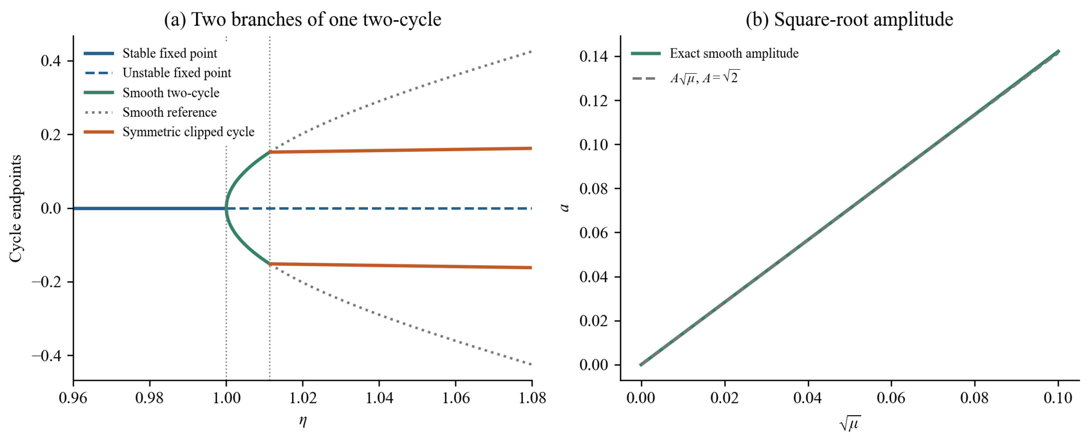
Figure 2.
Conceptual illustration of the flip-to-switching mechanism. (a) The ellipse represents the leading Euclidean approximation ; the two-cycle approaches opposite boundary points together. Higher-order midpoint drift is suppressed in this schematic. (b) The contact locus has quadratic separation from the flip locus. The scales are normalized and the plotted parabola represents the leading law, not a numerical continuation. The region above contact does not assert existence of clipped two-cycles.
Figure 2.
Conceptual illustration of the flip-to-switching mechanism. (a) The ellipse represents the leading Euclidean approximation ; the two-cycle approaches opposite boundary points together. Higher-order midpoint drift is suppressed in this schematic. (b) The contact locus has quadratic separation from the flip locus. The scales are normalized and the plotted parabola represents the leading law, not a numerical continuation. The region above contact does not assert existence of clipped two-cycles.
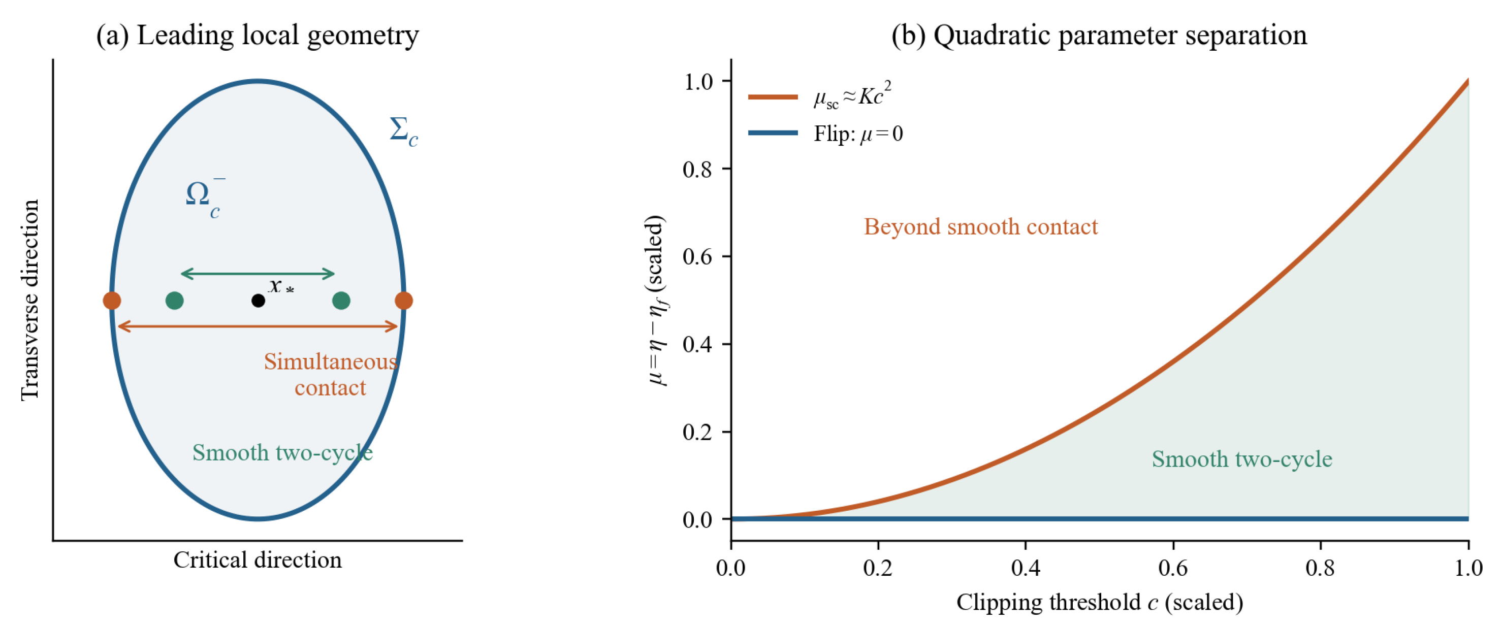
Figure 3.
Exact switching boundary in the planar model, , for the parameters of Figure 1. The horizontal and vertical axes have different scales. (a) The smooth cycle at lies inside the boundary. (b) At , both endpoints reach the boundary simultaneously. (c) At , the symmetric clipped cycle lies outside. Curved arrows denote discrete one-step exchange; they are not trajectory paths in the intervening region. Unlike Figure 2, the boundary and endpoints here are computed from exact model formulas.
Figure 3.
Exact switching boundary in the planar model, , for the parameters of Figure 1. The horizontal and vertical axes have different scales. (a) The smooth cycle at lies inside the boundary. (b) At , both endpoints reach the boundary simultaneously. (c) At , the symmetric clipped cycle lies outside. Curved arrows denote discrete one-step exchange; they are not trajectory paths in the intervening region. Unlike Figure 2, the boundary and endpoints here are computed from exact model formulas.
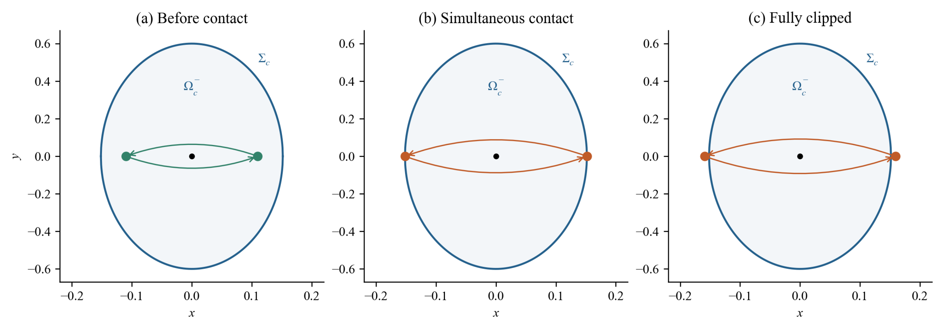
Figure 4.
Quantitative contact law in the solvable model. (a) The exact separation , with , is compared with for . (b) At fixed , the two smooth cycle points have the same exposure . Its intersection with determines the unique simultaneous contact. All curves use analytic formulas and scalar root solving, without fitted coefficients.
Figure 4.
Quantitative contact law in the solvable model. (a) The exact separation , with , is compared with for . (b) At fixed , the two smooth cycle points have the same exposure . Its intersection with determines the unique simultaneous contact. All curves use analytic formulas and scalar root solving, without fitted coefficients.
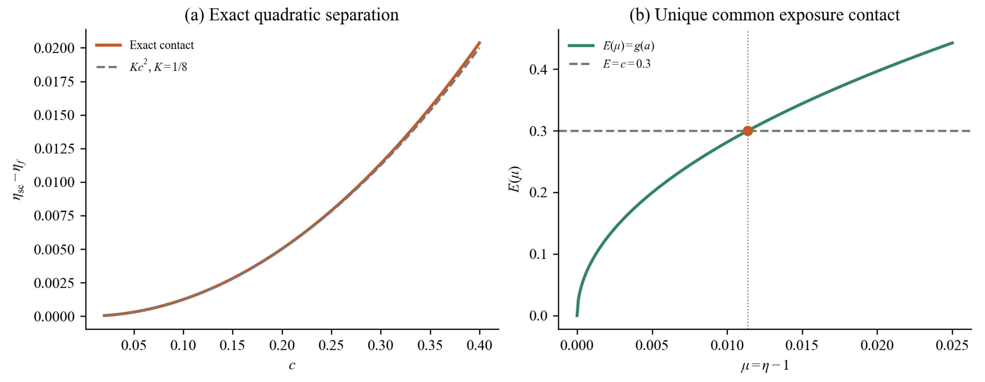
Figure 5.
Iterates of the actual clipped scalar map on the invariant axis, , with the parameters of Figure 1. (a,b) Cobweb rectangles show the one-step exchange of the two endpoints for a smooth cycle at and an asymmetric clipped cycle at . (c) Both trajectories alternate between two values; the smooth trajectory uses 1752 burn-in steps, while the clipped trajectory starts at and is exactly periodic. (d) From , decays to zero below the flip () and approaches the smooth cycle amplitude above it. Connecting segments in (c) show iteration order, not a continuous-time flow.
Figure 5.
Iterates of the actual clipped scalar map on the invariant axis, , with the parameters of Figure 1. (a,b) Cobweb rectangles show the one-step exchange of the two endpoints for a smooth cycle at and an asymmetric clipped cycle at . (c) Both trajectories alternate between two values; the smooth trajectory uses 1752 burn-in steps, while the clipped trajectory starts at and is exactly periodic. (d) From , decays to zero below the flip () and approaches the smooth cycle amplitude above it. Connecting segments in (c) show iteration order, not a continuous-time flow.
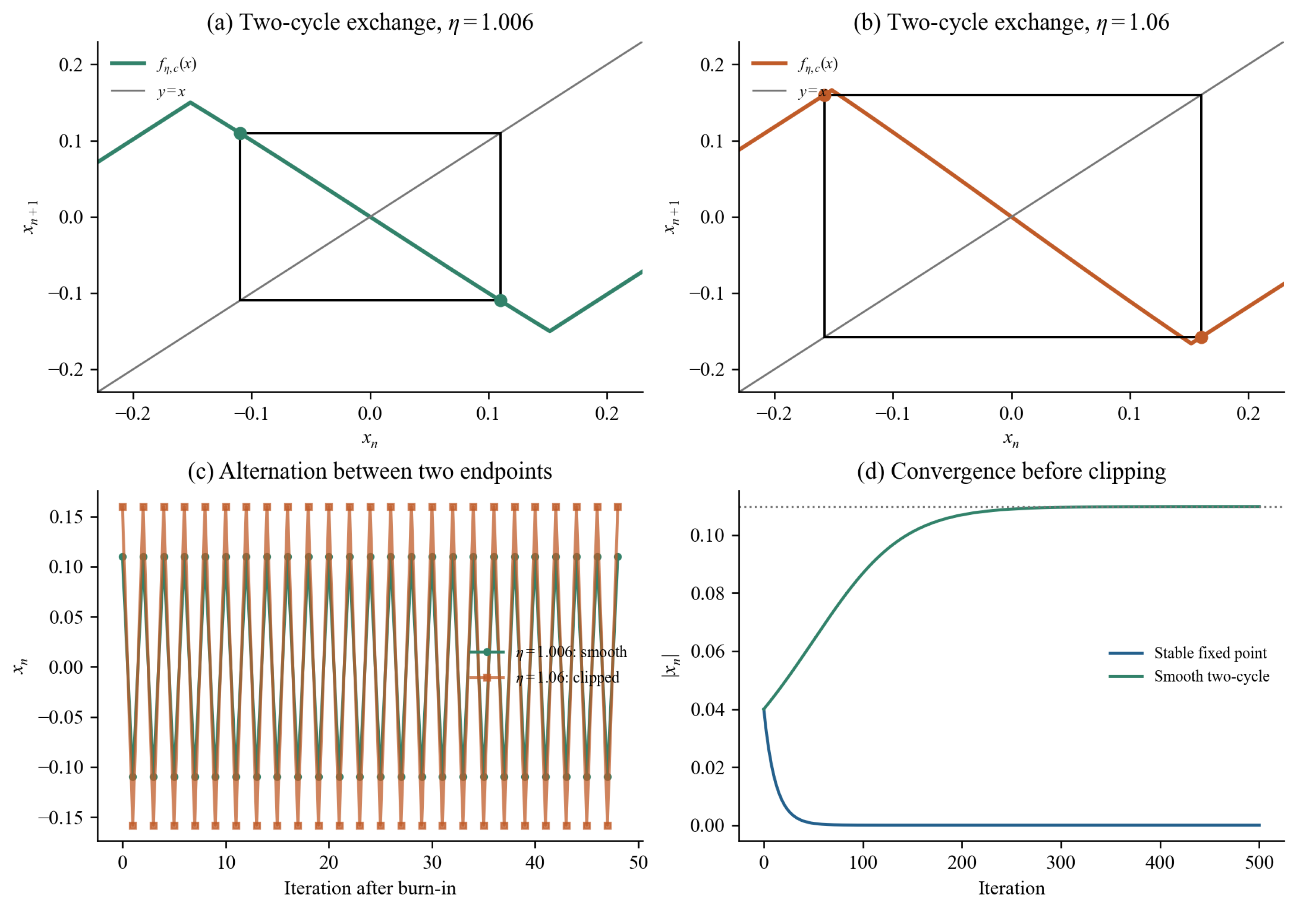
Figure 6.
Fully clipped family for and . Write and ; the interval is open. (a) Each value of s gives one cycle with endpoints and . (b) The two-step map is exactly the identity on the positive-endpoint interval. (c) The longitudinal multiplier is one throughout the family, while the exact transverse multiplier lies inside the unit disk for these parameters. Neutrality along the family therefore coexists with transverse contraction; no individual member is linearly exponentially attracting.
Figure 6.
Fully clipped family for and . Write and ; the interval is open. (a) Each value of s gives one cycle with endpoints and . (b) The two-step map is exactly the identity on the positive-endpoint interval. (c) The longitudinal multiplier is one throughout the family, while the exact transverse multiplier lies inside the unit disk for these parameters. Neutrality along the family therefore coexists with transverse contraction; no individual member is linearly exponentially attracting.
Disclaimer/Publisher’s Note: The statements, opinions and data contained in all publications are solely those of the individual author(s) and contributor(s) and not of MDPI and/or the editor(s). MDPI and/or the editor(s) disclaim responsibility for any injury to people or property resulting from any ideas, methods, instructions or products referred to in the content. |
© 2026 by the authors. Licensee MDPI, Basel, Switzerland. This article is an open access article distributed under the terms and conditions of the Creative Commons Attribution (CC BY) license (http://creativecommons.org/licenses/by/4.0/).
Copyright: This open access article is published under a Creative Commons CC BY 4.0 license, which permit the free download, distribution, and reuse, provided that the author and preprint are cited in any reuse.