
Submitted:
26 October 2026
Posted:
27 October 2026
You are already at the latest version
Abstract
The grain yield differences assessed between five cropping sectors in a rainfed spring wheat field in northern Kazakhstan by integrating data from yield measurements, soil chemistry, sensor telemetry, satellite-derived NDVI, and field hypsometry. Four sectors received the soil amendment SoilPoint (SPB), mineral nitrogen at 0–10 kg ha⁻¹, and reduced herbicide rates, the control sector received 20 kg N ha⁻¹ without SPB. Each cropping package covered one sector. Total sector yield reached 3.47 t ha⁻¹ in the SPB-N2 treatment compared to 2.57 t ha⁻¹ in the control sector, a difference of approximately 35%. The SPB-N2 treatment also demonstrated the highest postharvest yield and the highest local average soil moisture index (40.31%). With increasing altitude, average moisture indices decreased from 40.31% at 255–256 m to 35.84% above 258 m. Telemetry data revealed significant temporal variability in the shallow soil layers, with the decline from the first to the last week varying depending on the monitoring site. The highest average NDVI was observed in SPB-N10, and soil nutrient concentrations followed seasonal trajectories specific to each element. A comprehensive assessment links sector productivity to crop structure, soil chemistry, and local moisture dynamics within their topographic context. We hypothesize that elevation-related differences in moisture conditions contributed to the formation of crop yield patterns and that SPB-N2's leading position may be maintained over multiple seasons.
Keywords:
spring wheat
; field observation
; crop management measures
; soil agrochemistry
; sensorbased moisture index
; NDVI
; grain yield
1. Introduction
Yield variations in commercial wheat fields reflect management characteristics, weather conditions, and spatial variability in soil and topography. Statistical yield modeling and drought analysis demonstrate the importance of seasonal climate for wheat production in Kazakhstan [1,2]. Farm-level assessments identify production conditions as important sources of yield variation [3], while regional studies link changes in wheat production to climate trends [4]. Field-scale studies complement these regional assessments by examining yields in conjunction with soil and water-retention conditions.
A comprehensive field assessment integrates observations at complementary scales. Harvesting across the entire sector allows for grain production assessment, crop profiles characterize selected sampling sites, soil composites describe chemical conditions, and soil sensors monitor moisture dynamics in local profiles. A satellite-based NDVI index adds spatial information on vegetation greenness. Combining these measurements provides a basis for interpreting crop development in relation to management practices and the field environment.
In northern Kazakhstan, Diri et al. combined a comparative analysis of management practices at two sites with observations of plant cover and physiological parameters at different growth stages [5]. Their results link yield performance to grain formation under different tillage and weed control practices. Studies of yield components also show that grain quantity and grain weight compensate for each other differently under different conditions [6]. Thus, measurements of tillering, plant height, ear characteristics, and grain weight help explain how different crop structures influence final yield.
Water availability depends on soil depth, season, and field location. Research in northern Kazakhstan describes the role of soil moisture storage and crop water use [7], while experiments with dryland wheat demonstrate interactions between residue management, precipitation, and yield [8]. Experiments with herbicides and water stress further link moisture conditions to photosynthetic responses [9]. These results support a combined analysis of soil moisture, crop characteristics, and satellite data on vegetation condition.
The response to humic substances and other biostimulants depends on the composition, method of application, and environmental conditions [10,11]. Studies of humic acid-enriched urea [12] and commercial biostimulants under various conditions [13] demonstrate the value of assessing yield in conjunction with nutrient management. In the present study, SPB was part of a commercial management package combining product application, mineral nitrogen, and crop protection.
El-Hashash et al. assessed humic acid content under different water supply regimes at three sites over two seasons [14]. Their study demonstrates how moisture conditions and fertilizer management can be jointly studied. This approach is relevant for rainfed fields, where local soil moisture and topography provide additional spatial context for comparing crop yields.
Crop protection also influences yield variability. Zargar et al. investigated the reduction of herbicide application rates in combination with biological components in winter wheat [15]. Accordingly, the present analysis compares complete management packages, maintaining their SPB, mineral nitrogen, and crop protection components as part of the agronomic context of each sector.
Spatial analysis of field trials allows linking management decisions to patterned yield variation [16,17]. Joint soil and plant sensing, as well as Sentinel-2 time series, further characterize subfield heterogeneity [18,19]. The unit of comparison is the management sector, and plant samples, pixels, and repeated sensor readings describe variations within this unit [20].
The timing of crop cover observations also influences their relationship with yield. Studies of wheat using NDVI at specific crop ages link crop cover development to nitrogen uptake and grain formation [21]. Combining consistent data collection with soil measurements and crop observations helps determine the impact of NDVI on seasonal field development.
The aim of the study was to assess grain crop yields in the sector through a comprehensive analysis of crop characteristics, seasonal soil chemistry, local soil moisture, NDVI, and field hypsometry. We compared harvest results across the sector with estimates obtained at harvest, examined the correlation between soil and crop parameters and yield rankings, and analyzed sensor telemetry data depending on elevation differences. Particular attention was paid to the hypothesis that local moisture conditions, related to topography, influence the spatial structure of crop yields.
2. Materials and Methods
2.1. Field Study and Observation Design
The study was conducted in 2026 in field #21 near Bannovka, Fyodorovsky District, Kostanay Region, northern Kazakhstan. The field center is located at approximately 53.72915° N, 63.01309° E (Figure 1). Spring bread wheat ( Triticum aestivum L. ) of the ‘Granny’ variety, grown without irrigation, was grown. Five harvested plots totaled 197.15 hectares.
Daily precipitation data were obtained from iMetos 3.3 station 002131C1, located approximately 8.9 km southwest of the field center. The precipitation dataset for the period from May 22 to August 21 was analyzed in conjunction with soil sensor telemetry data to describe the timing of wetting and drying during the monitoring period.
Four elongated sectors received management packages based on the SPB method. The reference sector occupied 6.95 hectares on the southwestern edge of the field, while the sectors corresponding to the SPB method ranged from 42.35 to 53.80 hectares. Each management package covered one sector. The study used comparative observations of these five sectors, with sector position and management methods considered together when interpreting the results. Field hypsometry and sensor locations were analyzed using an elevation map. Sensors 1–4 corresponded to SPB-N0, SPB-N2, SPB-N6, and SPB-N10, respectively. Each sensor was assigned a corresponding elevation class, as indicated on the map. Relative elevation intervals were calculated from the class boundaries, using sensor 2, located at an elevation of 255–256 m, as the reference. The analysis combined these elevation differences with depth-resolved telemetry data, average profile moisture indices, and sectoral yield data.
Pre-sowing powder treatment was conducted from May 18th to 26th. Wheat was sown from June 3rd to 6th at a depth of 5–6 cm, with a second powder treatment at sowing. Plant protection measures and liquid SPB application were conducted on July 8th to 9th and August 2nd to 3rd. Soil sampling was conducted on June 8th, July 5th, and September 30th. Flag leaves were photographed on July 30th, and harvesting took place from September 25th to October 1st. Thus, the first soil survey was conducted after SPB application and sowing, and the final survey was conducted during harvest.
2.2. Management Tool Packages and Observation Methodology
Sector labels indicate mineral nitrogen applied as ammonium nitrate: 0, 2, 6, and 10 kg N ha−1 in SPB-N0, SPB-N2, SPB-N6, and SPB-N10, respectively, and 20 kg N ha−1 in the reference case. Table 1 presents the management packages. Table 2 provides a summary of the sampling design, seasonal coverage, and objectives of the observational analysis.
The powder application schedule included 12 kg/ha before sowing and 3 kg/ha during sowing, with a permissible error of ±1 kg/ha. Liquid SPB application rates were 6 l/ha followed by 12 l/ha in the SPB-N0 and SPB-N2 variants, and 4 l/ha followed by 8 l/ha in the SPB-N6 and SPB-N10 variants. The full crop protection program included Kaskad Premium at 0.025 kg/ha, Torres at 0.4 l/ha, Leggero Forte at 0.3 l/ha, and Neon 99 at 0.1 l/ha. The herbicide application rate was 30% of the full program in SPB-N0 and SPB-N2, 50% in SPB-N6 and SPB-N10, and 100% in the control group (Table 1). The overall program for August included Beskar at 0.3 l/ha and Espada at 0.12 l/ha.
Kaskad Premium contains tribenuron-methyl, thifensulfuron-methyl, and florasulam at concentrations of 410, 140, and 200 g kg−1, respectively. Leggero Forte contains clodinafop-propargyl at a concentration of 240 g L−1 and saper clokintocet-mexyl at a concentration of 60 g L−1 [22]. Torres contains thiophanate-methyl, tebuconazole, and triadimenol at concentrations of 250, 167, and 43 g L−1, respectively [23]. Neon 99 was used as an adjuvant.
2.3. Crop Measurements and Spatial Mapping of Yield
Sector-wide yield was calculated as the mass of harvested grain divided by the harvested area, Y = M/A, where M is the mass of grain in tons and A is the harvested area in hectares. The yield difference was expressed relative to the reference value of 2.57 t/ha as 100(Y − 2.57)/2.57. Combine harvesting data were used to describe the spatial structure of yield. The map reconstruction included 18,005 values assigned from color classes and 4,460 individually extracted values within the bounded area. Ordinary kriging in SAGA GIS 7.8.2 was used to reconstruct a continuous yield surface (Figure 4a). The spatial maps were examined together with sectoral yield values and NDVI imagery to identify patterns within and across management boundaries.
2.4. Diagnostic Sections of the Crop and Grain Measurements
Five 0.25 m2 harvest plots were collected in each sector, comprising 25 sampling points. Sampling locations were selected based on median and quartile NDVI values during the peak growing season. For each 0.25 m2 plot, yield in t/ha was calculated by multiplying the grain weight in grams by 0.04. The yield plot results for each sector were presented as arithmetic means and standard deviations within the sector.
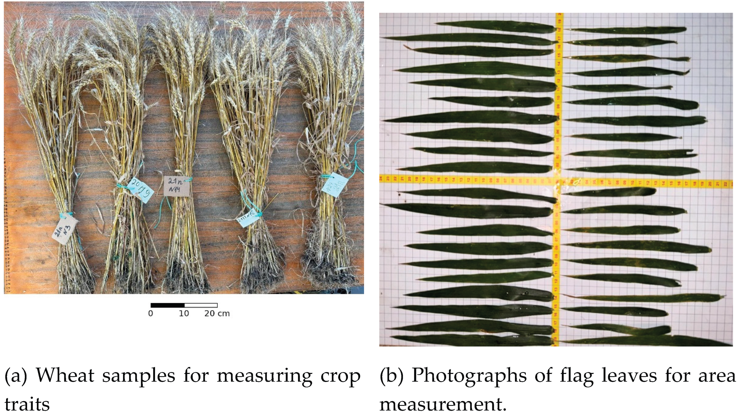
Productive tillering, plant height, spike characteristics, and thousand-kernel weight were measured on the harvest samples (Figure 2a). Productive tillering and thousand-kernel weight were summarized based on four observations in SPB-N0 and SPB-N2 and five in the other sectors. Individual plant measurements included 45–59 observations per sector. On July 30, 20 flag leaves from SPB-N0 and 20 from the control sample were photographed relative to a ruler and digitized in QGIS to determine leaf area (Figure 2b).
One sample of harvested grain was taken from each sector for analysis of protein content, moisture, specific gravity, falling number, wet gluten, and thousand-kernel weight. Grain quality parameters describe samples from the harvested lot. Thousand-kernel weights from the lot samples and from the slices were analyzed separately
Figure 2.
Yield measurements. (a) Wheat samples next to a ruler for assessing plant traits. (b) Flag leaves photographed against the background of the measuring grid and ruler for digitizing leaf area in SPB-N0 and the reference sector.
Figure 2.
Yield measurements. (a) Wheat samples next to a ruler for assessing plant traits. (b) Flag leaves photographed against the background of the measuring grid and ruler for digitizing leaf area in SPB-N0 and the reference sector.
2.5. Comprehensive Soil Sampling and Laboratory Analysis
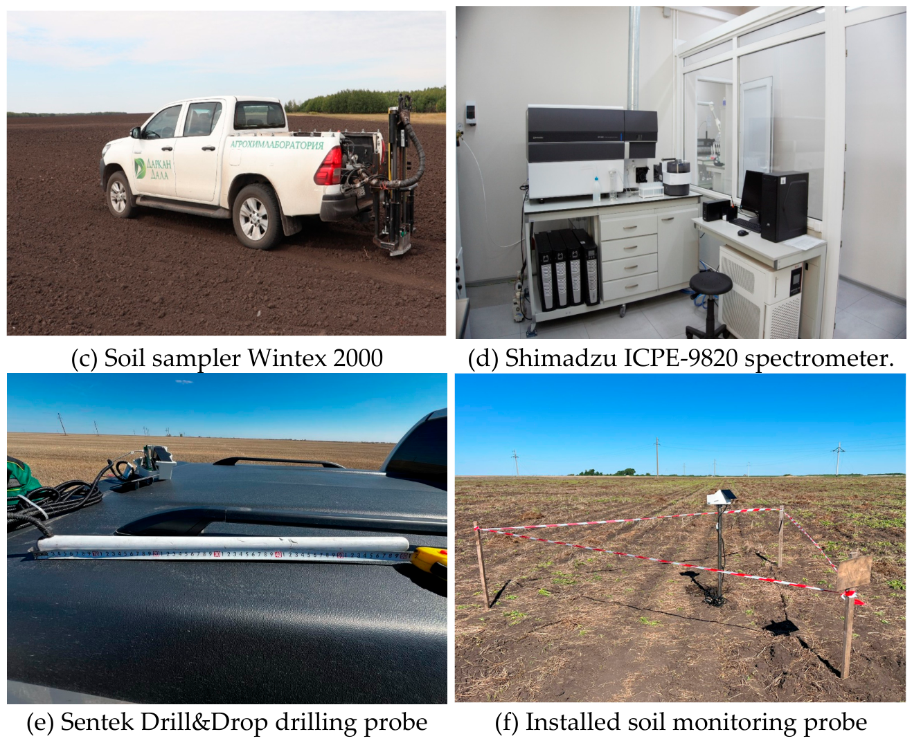
One composite soil sample was collected in each sector on June 8, July 5, and September 30, 2026, yielding a total of 15 composite samples across sectors and dates. Nitrate nitrogen content was determined in the 0–20 cm soil layer. Soil samples were collected using a Wintex 2000 sampler mounted on a vehicle, pooled, labeled, and transported to the laboratory in sealed bags.
Soil analysis included determination of salt extract pH, nitrate nitrogen, P2O5, K2O, sulfur, humus, Ca, Mg, Cu, Fe, Mn, Mo, and Zn. Nutrient concentrations were expressed as mg kg−1, humus content as %, and pH as a dimensionless scale. Laboratory equipment included a Shimadzu ICPE-9820 spectrometer (Figure 3d).
Figure 3.
Sampling and monitoring equipment. (c) Wintex 2000 soil sampler truck. (d) Shimadzu ICPE-9820 spectrometer. (e) Sentek Drill&Drop 60cm probe during installation in field 64. (f) Installed telemetry station in field 21.
Figure 3.
Sampling and monitoring equipment. (c) Wintex 2000 soil sampler truck. (d) Shimadzu ICPE-9820 spectrometer. (e) Sentek Drill&Drop 60cm probe during installation in field 64. (f) Installed telemetry station in field 21.
2.6. Local Soil Moisture Monitoring
One 60-cm Sentek Drill&Drop probe was used to monitor each sector of SPB. The probes were distributed as follows: 1. station 1_21 (031137DD) — to SPB-N0, 2. station 2-21 (031137DC) — to SPB-N2, 3. station 3_21 (03113E1B) — to SPB-N6, and 4. station 4_21 (03113E2C) — to SPB-N10. Each probe recorded six channels at nominal depths of 10, 20, 30, 40, 50, and 60 cm. Daily averages from FieldClimate covered the period from 22 May to 21 August 2026: 92 dates, 368 probe-day profiles, and 2208 channel-day values (92 × 4 × 6). The local profile moisture index was calculated as I(t) = [θ10(t) + θ20(t) + θ30(t) + θ40(t) + θ50(t) + θ60(t)]/6, using the probe’s percentage scale. Period means and sample standard deviations summarized the 92 daily indices at each monitoring point. To summarize the depth data, the four sensors’ values were averaged for each date before calculating the mean value over the period and the standard deviation over time. Seasonal decline was calculated as the difference between the average index values for May 22–28 and August 15–21, expressed as percentage points. Daily telemetry data was analyzed without smoothing or interpolation.
2.7. Satellite Observations
The NDVI index was calculated based on 12 selected Sentinel-2 level 2A observations as (B08 − B04)/(B08 + B04). The observation set included three scenes in May preceding sowing and nine later scenes. The sectors summarize the green vegetation for the selected observation period. The spatial image of NDVI (Figure 4b) was used to study the heterogeneity of vegetation cover in the management sectors. The analysis took into account the influence of observation time, soil background, and vegetation development on NDVI [24].
2.8. Statistical Summaries and Comprehensive Analysis
Five management sectors served as units of descriptive comparison. Crop samples, plants, leaves, pixels, soil increment, and repeated sensor readings characterized variations within these units [20]. Crop slice results were summarized by within-sector means and standard deviations, and sensor indices were summarized by period means and time-dependent standard deviations. Pearson correlations described the relationships between precipitation and shallow water changes both within and with a one-day lag. A yield trait heat map standardized each trait across the five sectors using the population standard deviation, z = (x − mean)/SD, while preserving numeric values in cells. Soil chemistry was analyzed as a sequence of sector-date component concentrations. An integrated analysis compared sector rankings and associated moisture trajectories with mapped elevation differences.
3. Results
3.1. Profitability and Spatial Structure Across the Sector
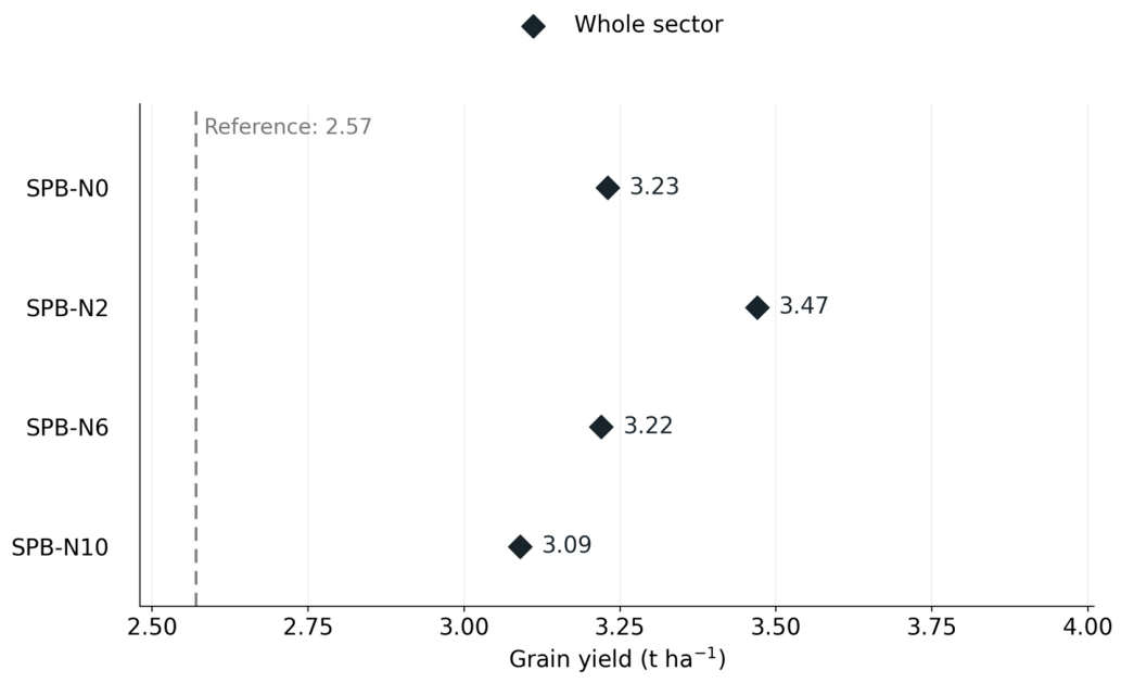
The yield of the entire sector was highest in the SPB-N2 variant and amounted to 3.47 t/ha compared to 2.57 t/ha in the control variant, a difference of 0.90 t/ha or approximately 35% (Table 3, Figure 6). Variants SPB-N0, SPB-N6, and SPB-N10 yielded 3.23, 3.22, and 3.09 t/ha, respectively, exceeding the control variant by approximately 26%, 25%, and 20%.
Figure 4.
Spatial patterns of crop yield (a) and NDVI (b) in field 21. The yield surface was reconstructed from color class values using ordinary kriging.
Figure 4.
Spatial patterns of crop yield (a) and NDVI (b) in field 21. The yield surface was reconstructed from color class values using ordinary kriging.
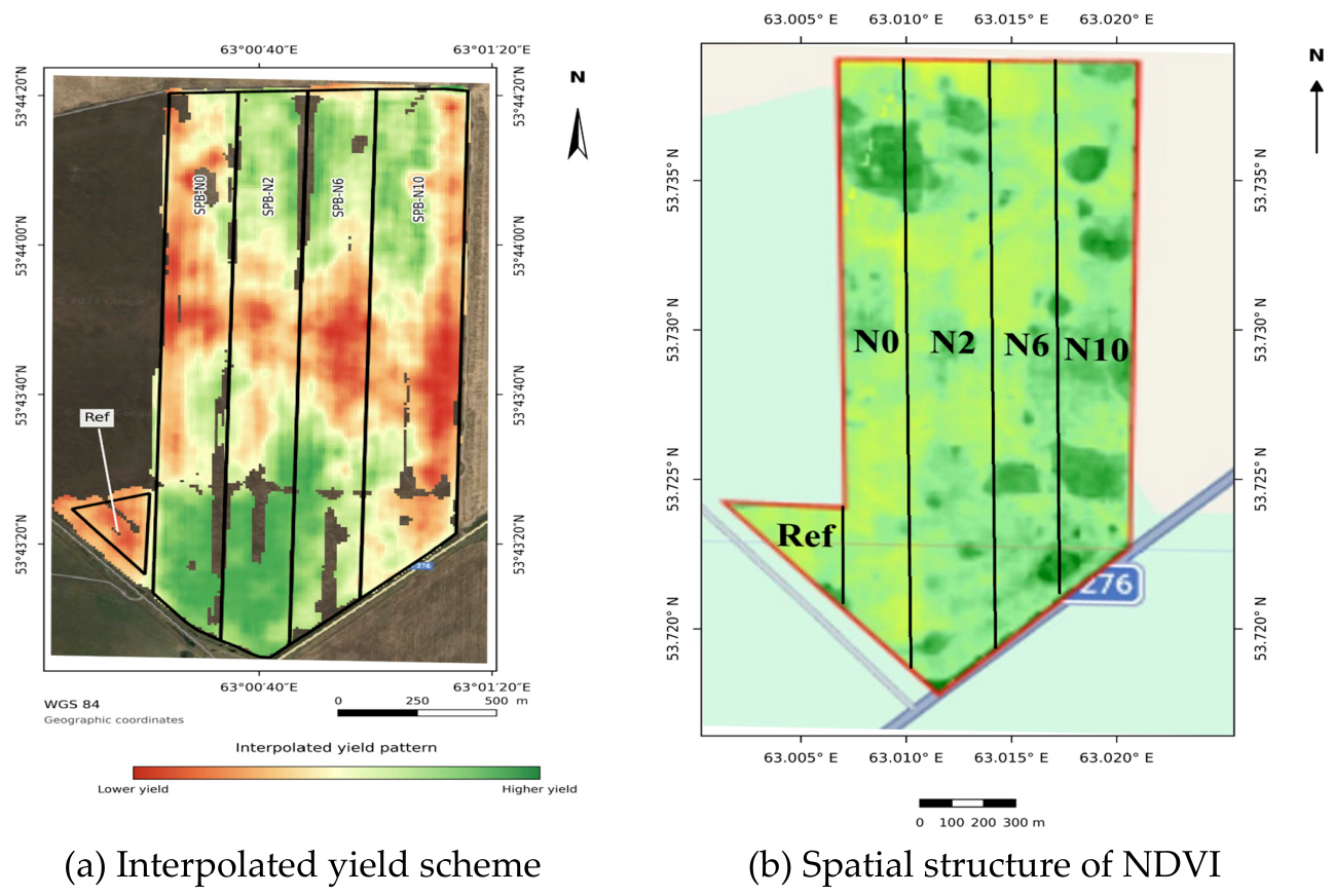
The yield map showed a band of lower yields crossing several tillage boundaries, with lower values near the field edges (Figure 4a). Higher values were observed in the southern portions of SPB-N0 and SPB-N2, located near the control point. The NDVI image also revealed heterogeneity within the field (Figure 4b). These patterns indicate that the comparison of yields across sectors occurs within a spatially variable field.
Figure 5.
Hypsometric map of field #21. Elevation classes: ≤254, 254–255, 255–256, 256–257, 257–258, and >258 m above sea level. Numbered markers indicate sensors 1–4, black lines show contours.
Figure 5.
Hypsometric map of field #21. Elevation classes: ≤254, 254–255, 255–256, 256–257, 257–258, and >258 m above sea level. Numbered markers indicate sensors 1–4, black lines show contours.
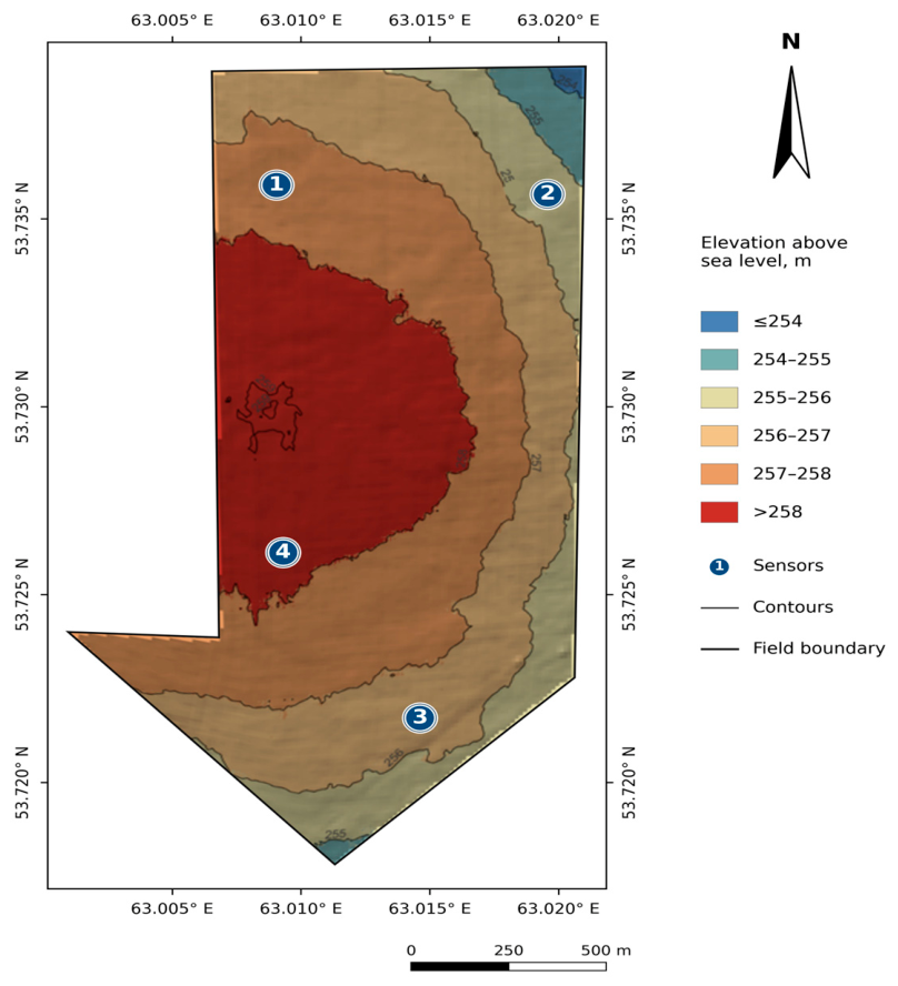
The field had a higher central-western part (>258 m) and lower northeastern and southern boundaries (Figure 5), with an elevation range exceeding 4 m. Sensor 1 occupied the northwestern 257–258 m class, sensor 2 the northeastern 255–256 m class, sensor 3 the southern 256–257 m class, and sensor 4 the southwestern >258 m class. These positions define the elevation gradient used in the telemetry analysis (Table 7).
Figure 6.
Grain yield across the entire sector. The dotted line represents the benchmark yield of 2.57 t/ha. Each dot represents one management sector.
Figure 6.
Grain yield across the entire sector. The dotted line represents the benchmark yield of 2.57 t/ha. Each dot represents one management sector.
Combine harvester yield data were 0.4–9.9% lower than scale-based yields, while color-class reconstructions differed by -3.2% to +6.2%. These comparisons describe the relationship between sectoral yield measurements and spatial yield reconstructions.
3.2. Diagnostic Sections of Crops and Measured Characteristics of Crops
The average post-cut yield was 1.18 ± 0.32 t ha−1 in the control, 2.56 ± 0.71 t in the SPB-N0, 3.28 ± 0.63 t in the SPB-N2, 3.00 ± 1.05 t in the SPB-N6, and 2.94 ± 0.35 t in the SPB-N10 (mean ± standard deviation within sector, five cuts per sector). Compared with the yield in the entire sector, the average post-cut yields were lower by 54.1%, 20.7%, 5.5%, 6.8%, and 4.9%, respectively (Table 3). The overall sector ranking was as follows: SPB-N2 > SPB-N0 > SPB-N6 > SPB-N10 > benchmark, the harvest ranking was as follows: SPB-N2 > SPB-N6 > SPB-N10 > SPB-N0 > benchmark. Both measurement methods identified the same sectors with the highest and lowest yields, with differences between the intermediate positions. The SPB-N0 cultivar had the highest average productive tillering of 1.79 ± 0.32 ears per plant, compared to 1.21 ± 0.10 for the control cultivar. The average flag leaf area was 20.49 ± 4.05 cm2 for SPB-N0 and 12.81 ± 3.04 cm2 for the control cultivar, a difference of approximately 60%. The SPB-N6 and SPB-N10 cultivars had more grains per spike, SPB-N2 had the highest median thousand-kernel weight in the yield samples (43.6 g), and SPB-N10 had the highest median plant height (71.5 cm, Figure 7). Thus, the yield ranking combined contrasting patterns of tillering, spike productivity, and grain weight.
3.3. Quality of Harvested Grain
Protein content ranged from 13.1% in the reference sample to 13.7% in the SPB-N2 sample, and wet gluten content ranged from 23.2% to 25.8% (Table 4). SPB-N2 combined the highest wet protein and gluten values with the highest overall yield. Thousand-kernel weights in the collected samples ranged from 41.4 to 53.6 g.

Table 4.
Quality of collected grain samples from each sector.
| Sector | Protein % | Wet gluten, % | Sample mass, g l−1 | Mass of a thousand grains, g |
|---|---|---|---|---|
| Link | 13.1 | 24.6 | 797 | 41.4 |
| SPB-N0 | 13.5 | 25.6 | 782 | 44.1 |
| SPB-N2 | 13.7 | 25.8 | 807 | 44.6 |
| SPB-N6 | 13.5 | 23.2 | 793 | 53.6 |
| SPB-N10 | 13.6 | 23.6 | 792 | 44.0 |
Each sector was represented by a single sample of harvested grain. The thousand-grain weight of lot SPB-N6 was 53.6 g, while the median weight of a harvest sample was 41.9 g. These values describe two separately collected groups of samples.
The moisture content of the analyzed grain samples ranged from 11.9% to 12.5%. Sample weight ranged from 782 to 807 g/l, with the highest value recorded in sample SPB-N2.
3.4. Seasonal Changes in Soil Nutrient Concentrations
At the first soil survey on 8 June, nitrate nitrogen concentrations were lowest in the SPB-N2 sector at 13.6 mg kg−1, compared to 20.1 mg in the control sector and 18.2–19.1 mg in the other SPB sectors. On 5 July, nitrate nitrogen concentrations reached 28.5 mg kg−1 in the control sector and 13.9 mg kg−1 in the SPB-N2 sector. By 30 September, concentrations were below June values in all sectors: 5.05 mg kg−1 in the control sector and 2.09–3.49 mg kg−1 in the SPB sectors, including 2.62 mg kg−1 in the SPB-N2 sector (Figure 8a). Thus, the highest yielding sector had the lowest nitrate nitrogen concentrations at the first survey, while September minimums were recorded in other SPB sectors.
In the SPB-N6 area, the P2O5 concentration was the highest on all three dates: 47.3, 54.6, and 30.7 mg kg−1 (Figure 8b). In the SPB-N0 area, it changed from 17.4 to 19.4 and to 18.3 mg kg−1 and was the only area where the September value exceeded the June value. Concentrations from June to September changed from 16.8 to 9.74 mg kg−1 in the control area, from 25.1 to 15.1 in the SPB-N2 area, and from 29.5 to 11.1 in the SPB-N10 area.
K2O concentrations decreased between June and September in all sectors (Figure 8c). SPB-N2 concentration changed from 697 to 725 and then to 611 mg kg−1 and maintained its highest concentration in September. Over the same period from June to September, SPB-N10 concentration changed from 912 to 340 mg kg−1, and SPB-N0 from 893 to 413 mg kg−1. Sulfur concentrations in September were also lower than June values in all sectors, ranging from 3.29 to 5.16 mg kg−1, while SPB-N2 and SPB-N6 reached a maximum in July (Figure 8d). In June, pH ranged from 5.8 to 6.8, and humus content ranged from 3.6% to 4.4% (Figure 8e,f). In September, pH was lower in all sectors. Humus content in SPB-N2 increased from 3.7% to 4.1%, while in the remaining sectors it was lower than in June.
Mg and Mn concentrations decreased from June to September in all sectors, while Ca and Zn concentrations increased (Table 5). Cu, Fe, and Mo concentrations followed sector-specific trajectories. For example, Fe concentration increased from 3.52 to 3.95 mg kg−1 in the control sector and decreased in the SPB sectors. Thus, seasonal chemical dynamics varied both among elements and between management sectors.
Table 5.
Concentrations of Ca, Mg and microelements in June and September 2026, mg kg−1.
| Sector | Ka | Mg | Cu | Fe | Mn | Mo | Zinc |
|---|---|---|---|---|---|---|---|
| Link | 3280 → 3420 | 604 → 483 | 0.15 → 0.17 | 3.52 → 3.95 | 10.3 → 6.56 | 0.10 → 0.21 | 0.68 → 1.26 |
| SPB-N0 | 3600 → 3670 | 572 → 431 | 0.21 → 0.14 | 3.77 → 1.92 | 15.1 → 6.48 | 0.21 → 0.04 | 0.87 → 3.61 |
| SPB-N2 | 3350 → 4200 | 588 → 527 | 0.14 → 0.17 | 1.98 → 1.73 | 10.6 → 5.44 | 0.15 →0.15 | 0.44 → 2.91 |
| SPB-N6 | 4870 → 5030 | 523 → 430 | 0.19 →0.19 | 2.31 → 2.10 | 19.6 → 8.59 | 0.09 → 0.13 | 0.53 → 2.58 |
| SPB-N10 | 4310 → 4530 | 528 → 424 | 0.33 → 0.18 | 2.47 → 1.86 | 15.3 → 7.39 | 0.11 → 0.14 | 0.45 → 1.29 |
The arrows indicate concentrations as of June 8 and September 30 for each sector. Each study was represented by one summary sample for each sector.
3.5. Telemetry of Soil Moisture and Precipitation
Across the four monitoring points, the average sensor readings at nominal depths of 10, 20, 30, 40, 50, and 60 cm were 18.60%, 30.23%, 39.51%, 44.21%, 45.92%, and 44.96%, respectively (Figure 9b). The temporal standard deviations of the average daily readings from the four sensors were 11.57 and 11.46 percentage points at depths of 10 and 20 cm, compared to 3.05 and 3.55 at depths of 50 and 60 cm. Consequently, the moisture signals in the shallow layer showed greater temporal variability than those in the deeper layers.
Probe 2 showed the highest average readings at depths of 10–50 cm, while Probe 4 showed the highest average readings at 60 cm. Figure 9b shows a wetting pulse at the end of the monitoring period, followed by a subsequent drying period. Short-term fluctuations were strongest in shallow channels, while trajectories in deeper layers changed more gradually. Thus, moisture dynamics varied both with monitoring position and depth.
The average humidity index values for the local profile were 36.20% in SPB-N0, 40.31% in SPB-N2, 36.60% in SPB-N6, and 35.84% in SPB-N10. Their temporal standard deviations were 6.60, 6.91, 5.13, and 8.06 percentage points, respectively. SPB-N2 showed the highest average value over the period, while SPB-N10 demonstrated the greatest temporal dispersion.
From the first to the last week of monitoring, the average index values decreased from 42.54% to 26.16% in SPB-N0, from 48.30% to 34.50% in SPB-N2, from 43.07% to 32.03% in SPB-N6, and from 43.95% to 22.66% in SPB-N10. These changes corresponded to decreases of 16.38, 13.80, 11.04, and 21.29 percentage points, respectively. SPB-N2 saw the highest average values for the first and last weeks, while SPB-N6 saw the smallest decrease.
The weather station recorded 192.8 mm of precipitation over the 92-day monitoring period, with rain falling on 40 days (Figure 9a). The highest daily precipitation total, 38.0 mm, on May 30 coincided with a 14.39 percentage point increase in the average measured by four sensors to 10 cm. A 27.8 mm precipitation on June 9 preceded an 11.34 percentage point increase on June 10.
For the average value obtained by four sensors at a depth of 10 cm, S(t), the diurnal change was ΔS(t) = S(t) − S(t − 1). The Pearson correlation coefficients were r[P(t), ΔS(t)] = 0.487 and r[P(t − 1), ΔS(t)] = 0.498, each based on 91 pairs of diurnal values. A positive one-day lag indicates the amount of precipitation preceding the change in sensor readings. The level correlation coefficient r[P(t), S(t)] was 0.191 based on 92 pairs. The calculations included both rainy and dry days. Thus, precipitation amount was more closely related to diurnal changes in shallow-water signals than to their absolute diurnal level.
3.6. Joint Assessment of Crop Yield, Soil Condition, Moisture and Hypsometry
SPB-N2 combined the highest overall yield across the sector with the highest local average moisture index, while SPB-N10 had the lowest values of both indices among the SPB sectors (Table 6). SPB-N6 had a slightly higher moisture index than SPB-N0 (36.60% versus 36.20%), with nearly equal yields across the sectors—3.22 and 3.23 t ha−1. The average NDVI was highest in SPB-N10—0.40—compared to 0.37 in SPB-N2. In the reference variant and SPB-N6, the rounded average NDVI was 0.36, despite the different yields. Thus, these indices describe different aspects of crop productivity and soil condition.
Figure 9.
Precipitation and soil moisture telemetry for the period 22 May to 21 August 2026. (a) Daily precipitation at iMetos 3.3 station 002131C1, located approximately 8.9 km southwest of the field center. (b) Daily sensor readings at six nominal depths in each SPB sector. Colors and axis boundaries are the same for all panels, and lines connect daily values on a percentage scale of sensor readings.
Figure 9.
Precipitation and soil moisture telemetry for the period 22 May to 21 August 2026. (a) Daily precipitation at iMetos 3.3 station 002131C1, located approximately 8.9 km southwest of the field center. (b) Daily sensor readings at six nominal depths in each SPB sector. Colors and axis boundaries are the same for all panels, and lines connect daily values on a percentage scale of sensor readings.
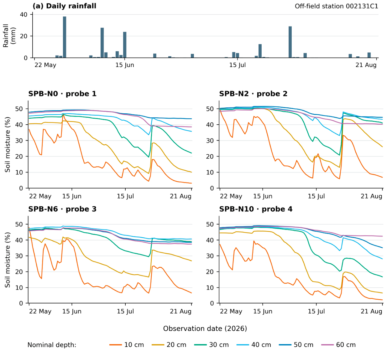
Table 6.
Yield by sector, nitrate nitrogen content, NDVI index and local soil moisture index.
| Sector | Yield across the sector, t ha−1 |
Nitrate nitrogen June 8 mg kg−1 |
Nitrate nitrogen 30 sen mg kg−1 |
Average NDVI value | obtained using a local sensor (%) |
|---|---|---|---|---|---|
| Link | 2.57 | 20.1 | 5.05 | 0.36 | Not controlled |
| SPB-N0 | 3.23 | 18.2 | 3.49 | 0.38 | 36.20 |
| SPB-N2 | 3.47 | 13.6 | 2.62 | 0.37 | 40.31 |
| SPB-N6 | 3.22 | 19.1 | 2.09 | 0.36 | 36.60 |
| SPB-N10 | 3.09 | 18.5 | 2.20 | 0.40 | 35.84 |
Yield reflects the yield of the entire sector. Nitrate nitrogen content is a single composite indicator ranging from 0 to 20 cm for each sector and sampling date. NDVI is the average of 12 selected observations, including three pre-sowing images. Moisture index is the average value of a six-channel profile index over 92 days at a monitoring point in each SPB sector.
On June 8, the profile moisture indices were 43.54%, 48.36%, 41.80%, and 43.86% in samples SPB-N0, SPB-N2, SPB-N6, and SPB-N10, respectively. On July 5, they were 37.87%, 39.25%, 35.37%, and 39.01%. Sample SPB-N2 ranked first, and SPB-N10 ranked second on both soil sampling dates. Over the same period, the nitrate nitrogen content changed from 13.6 to 13.9 mg kg−1 in sample SPB-N2, from 18.2 to 12.0 in sample SPB-N0, and from 18.5 to 16.3 in sample SPB-N10. Paired dates show how local moisture conditions and soil nitrogen concentrations changed at the beginning and middle of the observation period.
The altitude gradient provided a spatial basis for comparing telemetry data (Table 7). Sensor 2, located at 255–256 m in the northeast, showed the highest period average (40.31%) and the last week average (34.50%). Sensor 3, located at 256–257 m in the south, showed the smallest decreases in the first and last weeks (11.04 percentage points). Sensor 4, located above 258 m in the southwest, showed the lowest period average (35.84%) and the largest decrease (21.29 percentage points). Depending on the altitude, the period averages were 40.31%, 36.60%, 36.20%, and 35.84%.
The difference between readings from sensors 2 and 4 over the period was 4.47 percentage points. This difference increased from 4.35 percentage points in the first week to 11.84 in the final week. The corresponding yield values by sector differed by 0.38 t/ha. These results link the difference in elevation to different seasonal moisture trajectories and the corresponding productivity of the sectors.
Table 7.
Sensor location height, humidity dynamics in the area and sector yield.
| Sensor/sector | Location and altitude on the map, m | Δz above sensor 2, m | Average local index, % | First → last week, % | Decline, p. | Sector yield, t ha−1 |
|---|---|---|---|---|---|---|
| 1/SPB-NO | Northwest, 257–258 | about 1-3 | 36.20 | 42.54 → 26.16 | 16.38 | 3.23 |
| 2/SPB-N2 | Northeast, 255–256 | 0 (standard) | 40.31 | 48.30 → 34.50 | 13.80 | 3.47 |
| 3/SPB-N6 | South, 256–257 | approximately 0–2 | 36.60 | 43.07 → 32.03 | 11.04 | 3.22 |
| 4/SPB-N10 | Southwest, >258 | >2 | 35.84 | 43.95 → 22.66 | 21.29 | 3.09 |
Elevation classes correspond to Figure 5. Δz denotes the intervals of elevation difference relative to sensor 2 from the boundaries of the displayed class, and pp denotes percentage points. The first and last weeks are May 22–28 and August 15–21. Moisture indices describe local profiles, while crop yield describes entire sectors.
4. Discussion
4.1. Agreement Between Yield Measurements
The SPB-N2 variety took first place in both overall sector yield and post-harvest yield, while the reference variety placed last. Overall sector yields for the SPB-N0 and SPB-N6 varieties were virtually identical, differing by only 0.01 t/ha. The post-harvest yield ranking at the intermediate stage differed from the overall sector yield ranking. Taken together, these measurements allow us to identify distinct top and bottom positions in the field and a tighter grouping of the intermediate sectors.
The average harvest loss was 54.1% lower than the entire sector yield in the reference variant and 5.5% lower in the SPB-N2 variant. The harvest loss values were specific to sites selected based on the NDVI index, while the harvested grain weight covered the entire sector. The magnitude of this difference demonstrates the importance of sampling location and area when comparing local yields with field production.
Thus, we consider sector-wide yield as the primary production outcome, and harvest data as additional indicators of yield formation at the local level. Using these indicators together allows us to link the final yield to crop characteristics measured at sampling sites.
4.2. Field Location and Spatial Structure of Crop Yield
The field locations provide agronomic context for the yield comparison. The reference plot occupied 6.95 hectares on the southwestern edge, while each of the SPB sectors exceeded 42 hectares and extended along various transects. The yield structure crossed several management boundaries, and the hypsometric map revealed contrasting upper and lower positions. These spatial features support an interpretation that takes into account both topography and management practices.
Cho et al. related the response of strips on a farm to adjacent control plots and historical yield zones [16], while Laws and Bramley used explicit spatial comparisons in farm-scale trials [17]. Their approaches emphasize the role of field structure in management assessment. In the present study, five industry summaries, spatial yield structure, and monitoring positions provide additional insights into this structure [20].
4.3. Characteristics of Agricultural Crops and Dynamics of Soil Chemical Composition
Crop characteristics indicate contrasting grain formation pathways. SPB-N0 had the greatest tillering and flag leaf area than the control, SPB-N2 had the highest median thousand-grain weight across the crop accessions, and SPB-N10 had the highest median plant height. Compensation between yield components suggests an agronomic interpretation of these differences [6]. Moisture experiments tracking assimilate redistribution further link soil moisture conditions to grain formation [25], supporting the feasibility of integrated consideration of crop structure and profile moisture dynamics.
Soil chemistry trajectories describe the seasonal nutrient environment accompanying crop growth. Nutrient concentrations, nutrient storage in the soil, and plant uptake represent individual components of nutrient dynamics. Studies of phosphorus recovery [26] and nitrogen fate [12,27] demonstrate the value of linking these components, while soil analysis interpretation relates each analytical fraction to its extraction method [28]. Here, concentrations by sector and date characterize the chemical conditions at three sampling stages.
The highest yield in SPB-N2 coincided with the lowest nitrate nitrogen concentration during the initial survey. The highest P2O5 and K2O concentrations in June were observed in other sectors. Thus, yield development corresponded to the combined condition of the crop and soil, rather than to an overall maximum for all measured nutrients. The seasonal decline in the concentrations of several nutrients is consistent with changing nutrient dynamics during crop development.
The dynamics of individual element contents further differentiated the sectors. The contents of N, K, S, Mg, and Mn generally decreased from June to September, while those of Ca and Zn increased. The dynamics of humus and microelement contents varied between sectors. These results support a differentiated assessment of soil chemistry, considering each element within its seasonal and spatial context.
4.4. Hypsometry, Humidity Dynamics and the Green Phase of Plants
Average humidity index values decreased with increasing altitude: from 40.31% at the northeastern elevation of 255–256 m to 35.84% at the southwestern elevation of over 258 m. We hypothesize that topographically related moisture redistribution and conservation contributed to this pattern. Telemetry adds a seasonal dimension: the greatest decrease was observed at sensor 4, while the smallest was at sensor 3, located at an elevation of 256–257 m. Thus, local humidity conditions combine an altitude gradient with various temporal variations.
McDonald et al. identified the topographic position index as a stronger predictor of yield than absolute elevation in their wheat model [29]. This finding places the present comparison of elevation classes in the broader context of the role of landscape position in dryland grain production. In field 21, the elevation map defines the spatial gradient, and a series of sensors describes the moisture response at each monitored point.
Compared to sensor 2, the elevation differences were approximately 1–3 m for sensor 1, 0–2 m for sensor 3, and over 2 m for sensor 4 (Table 7). The depth-dependent curves show how the profiles varied along this gradient. Shallow channels showed greater fluctuations, with sensor 4 showing the highest average value—60 cm—despite having the lowest average profile. Thus, the relationship between elevation and moisture content is best interpreted based on both the average profile state and the dynamics of individual layers.
The increase in the difference between sensors 2 and 4, from 4.35 percentage points in the first week to 11.84 in the last, is consistent with the contrasting seasonal behavior of moisture in the lower and upper positions. Soil profile sensors describe these changes through depth-specific dielectric responses [30]. We interpret the simultaneous presence of higher moisture indices and higher yields in SPB-N2 as confirmation of the possible contribution of local moisture conditions to crop productivity under combined topography, soil, and management conditions.
NDVI adds information about the greenness of the canopy during its collection. Marino linked NDVI dynamics at individual sites to growth stages and landscape position [19], while Mitra et al. linked crop age-specific NDVI to nitrogen management in wheat [21]. In this field, the highest average NDVI over the sample period was recorded at SPB-N10, while SPB-N2 had the highest grain yield. This difference highlights the complementary roles of canopy greenness and final grain yield, as well as the importance of observation timing and soil background [24,31].
4.5. Complex Translation
The comprehensive assessment links grain production to crop structure, soil chemistry, moisture dynamics, and topography. SPB-N2 combined the highest sector yields, harvest yields, median grain weight in harvest samples, and local average moisture index. Other sectors demonstrated superior tillering, height, NDVI, and individual soil nutrients. This combination demonstrates that sector productivity reflects multiple aspects of the crop-soil system.
Mazur et al. linked soil composites and satellite observations within management zones [18]. The proposed combination extends this logic by incorporating depth-resolved telemetry and elevation differences. Soil surveys describe chemical conditions on selected dates, sensors describe daily profile dynamics, and NDVI describes the green zone of vegetation canopy throughout the entire data collection sequence. Together, these observations provide an agronomic understanding of the spatial structure of crop yields.
The leading position of SPB-N2 underlies the hypothesis that yield rankings are maintained across multiple seasons. Multi-environment on-farm comparisons demonstrate how management measures vary across production conditions [13], while a meta-analysis of biostimulants demonstrates the role of environmental and application conditions [11]. Product-specific assessment also includes nutrient composition and management when interpreting commercial biostimulants [32]. We hypothesize that the combination of management practices and favorable local moisture conditions observed in SPB-N2 can ensure comparable performance in subsequent seasons.
5. Conclusions
A comprehensive field assessment allowed us to draw the following conclusions.
1. SPB-N2 demonstrated the highest yield overall in the sector—3.47 t/ha, compared to 2.57 t/ha in the control sample, a difference of approximately 35%. It also ranked first in yield after harvesting. Both methods identified the same sectors with the highest and lowest yields, while the intermediate indicators differed.
2. Average moisture index values decreased with increasing altitude. Sensor 2, at an altitude of 255–256 m, showed the highest average value (40.31%), while sensor 4, above 258 m, showed the lowest average value (35.84%) and the largest seasonal decrease. Sensor 3, at an altitude of 256–257 m, showed the smallest decrease. These patterns support the hypothesis that elevation-related moisture conditions influenced the spatial structure of crop yield.
3. Soil nutrient concentrations followed seasonal trajectories specific to each element, and the highest NDVI values and individual nutrient concentrations were observed in sectors other than the yield leader. A combined analysis of crop characteristics, soil chemistry, and sensor telemetry data provides a more comprehensive interpretation of sector productivity than any single indicator.
4. The SPB-N2 results support the hypothesis that the leading position in yield will be maintained over several seasons. This hypothesis links the crop management measures with local moisture conditions and hypsometric conditions.
Author Contributions
Conceptualization, BR, Methodology, BR and DT, Validation, MM, Formal analysis, BR, Investigation and data preparation, MM and AS, Writing – original draft, BR and AS, Writing – review and editing, BR, Visualization, BR, MM and AS, Scientific supervision and project administration, BR.
Funding
The relevant soil and environmental monitoring activities were supported by the Ministry of Science and Higher Education of the Republic of Kazakhstan under grant AP23485181 “Analysis of Soil Moisture Reserves Based on Satellite Imagery and Field Data, 2024–2026.” The SPB product, its manufacturer, or supplier were not funded by this grant.
Ethics Committee Statement
Not applicable, the study did not include human or animal participants.
Data Availability
The sectoral data analysed in this study are presented in tables and figures.
Conflicts of Interest
BR, and MM are employees of Darkan-Dala Agrochemical Company LLP, which participated in the field and analytical work. The manufacturer and supplier of SPB are not affiliated with Darkan-Dala and have no connection to grant AP23485181.
Use of artificial intelligence
OpenAI ChatGPT was used for language review of the manuscript and preparation of illustrations.
References
- Romanovska, P., Schauberger, B., Gornott, C. Wheat yields in Kazakhstan can successfully be forecasted using a statistical crop model. European Journal of Agronomy 2023, 147, 126843. [CrossRef]
- Karatayev, M., Clarke, M., Salnikov, V., Bekseitova, R., Nizamova, M. Monitoring climate change, drought conditions and wheat production in Eurasia: the case study of Kazakhstan. Heliyon 2022, 8(1), e08660. [CrossRef]
- Kurmanov, N., Baygabulova, K., Karbetova, Sh. Assessment of the impact of changes in production conditions on wheat yield capacity level. Problems of AgriMarket 2017, 2, 81–86. (In Russian). https://www.jpra-kazniiapk.kz/jour/article/view/1353.
- Romanovska, P., Undorf, S., Schauberger, B., Duisenbekova, A., Gornott, C. Human-induced climate change has decreased wheat production in northern Kazakhstan. Environmental Research: Climate 2024, 3(3), 031005. [CrossRef]
- Diri, K.H., Stybayev, G., Zargar, M., Baitelenova, A., Amantayev, B., Kulzhanova, S., Kulzhabayev, Y., Yelnazarkyzy, R. Soil management and weed control affect wheat productivity and resilience in semi-arid systems. AIMS Agriculture and Food 2026, 11(2), 300–319. [CrossRef]
- Slafer, G.A., Savin, R., Sadras, V.O. Coarse and fine regulation of wheat yield components in response to genotype and environment. Field Crops Research 2014, 157, 71–83. [CrossRef]
- Funakawa, S., Nakamura, I., Akshalov, K., Kosaki, T. Water dynamics in soil-plant systems under grain farming in Northern Kazakhstan. Soil Science and Plant Nutrition 2004, 50(8), 1219–1227. [CrossRef]
- Zhang, P., Wei, T., Wang, H., Wang, M., Meng, X., Mou, S., Zhang, R., Jia, Z., Han, Q. Effects of straw mulch on soil water and winter wheat production in dryland farming. Scientific Reports 2015, 5, 10725. [CrossRef]
- Todorova, D., Aleksandrov, V., Anev, S., Sergiev, I. Photosynthesis Alterations in Wheat Plants Induced by Herbicide, Soil Drought or Flooding. Agronomy 2022, 12(2), 390. [CrossRef]
- Rose, M.T., Patti, A.F., Little, K.R., Brown, A.L., Jackson, W.R., Cavagnaro, T.R. A meta-analysis and review of plant-growth response to humic substances: Practical implications for agriculture. In Advances in Agronomy, Sparks, D.L., Ed., Academic Press: San Diego, CA, USA, 2014, Vol. 124, pp. 37–89. [CrossRef]
- Li, J., Van Gerrewey, T., Geelen, D. A Meta-Analysis of Biostimulant Yield Effectiveness in Field Trials. Frontiers in Plant Science 2022, 13, 836702. [CrossRef]
- Gao, S., Zhang, S., Yuan, L., Li, Y., Wen, Y., Xu, J., Hu, S., Zhao, B. Humic Acids Incorporated into Urea at Different Proportions Increased Winter Wheat Yield and Optimized Fertilizer-Nitrogen Fate. Agronomy 2022, 12(7), 1526. [CrossRef]
- Izquierdo, J., Arriagada, O., García-Pintos, G., Ortiz, R., García-Pintos, M., García-Pintos, M. Humic field biostimulation as a sustainable agricultural practice to increase yield of main grains: evidence from on-farm trials. Frontiers in Plant Science 2025, 16, 1709876. [CrossRef]
- El-Hashash, E.F., Abou El-Enin, M.M., Abd El-Mageed, T.A., Attia, M.A.E.-H., El-Saadony, M.T., El-Tarabily, K.A., Shaaban, A. Bread Wheat Productivity in Response to Humic Acid Supply and Supplementary Irrigation Mode in Three Northwestern Coastal Sites of Egypt. Agronomy 2022, 12(7), 1499. [CrossRef]
- Zargar, M., Pakina, E.N., Plushikov, V.G., Vvedenskiy, V., Bayat, M. Efficacy of reducing lintour doses and biocontrol components for an effective weeds control in winter wheat (Triticum aestivum). Bulgarian Journal of Agricultural Science 2017, 23(6), 980–987. https://www.agrojournal.org/23/06-14.pdf.
- Cho, J.B., Guinness, J., Kharel, T., Maresma, Á., Czymmek, K.J., van Aardt, J., Ketterings, Q.M. Proposed Method for Statistical Analysis of On-Farm Single Strip Treatment Trials. Agronomy 2021, 11(10), 2042. [CrossRef]
- Lawes, R.A., Bramley, R.G.V. A simple method for the analysis of on-farm strip trials. Agronomy Journal 2012, 104(2), 371–377. [CrossRef]
- Mazur, P., Gozdowski, D., Wnuk, A. Relationships between Soil Electrical Conductivity and Sentinel-2-Derived NDVI with pH and Content of Selected Nutrients. Agronomy 2022, 12(2), 354. [CrossRef]
- Marino, S. Assessing the Agronomic Subfield Variability by Sentinel-2 NDVI Time-Series and Landscape Position. Agronomy 2023, 13(1), 44. [CrossRef]
- Hurlbert, S.H. Pseudoreplication and the design of ecological field experiments. Ecological Monographs 1984, 54(2), 187–211. [CrossRef]
- Mitra, B., Singha, P., Roy Chowdhury, A., Sinha, A.K., Skalicky, M., Brestic, M., Alamri, S., Hossain, A. Normalized difference vegetation index sensor-based nitrogen management in bread wheat (Triticum aestivum L.): Nutrient uptake, use efficiency, and partial nutrient balance. Frontiers in Plant Science 2023, 14, 1153500. [CrossRef]
- First Agrochemical Company. Product Catalogue 2025. Available online: https://atlantisagro.kz/wp-content/uploads/2025/02/Catalog2025.pdf (accessed 24 October 2026).
- First Agrochemical Company. Torres Product Information. Available online: https://1agro.kz/wp-content/uploads/2022/01/torres_2020.pdf (accessed 24 October 2026).
- Raun, W.R., Solie, J.B., Johnson, G.V., Stone, M.L., Lukina, E.V., Thomason, W.E., Schepers, J.S. In-season prediction of potential grain yield in winter wheat using canopy reflectance. Agronomy Journal 2001, 93(1), 131–138. [CrossRef]
- Zhang, Z., Yu, Z., Shi, Y., Zhang, Y. Effects of soil moisture on 13C assimilate redistribution and grain yield components in wheat. Frontiers in Plant Science 2025, 16, 1527224. [CrossRef]
- Shafi, M.I., Adnan, M., Fahad, S., Wahid, F., Khan, A., Yue, Z., Danish, S., Zafar-ul-Hye, M., Brtnicky, M., Datta, R. Application of Single Superphosphate with Humic Acid Improves the Growth, Yield and Phosphorus Uptake of Wheat (Triticum aestivum L.) in Calcareous Soil. Agronomy 2020, 10(9), 1224. [CrossRef]
- Koch, M., Akshalov, K., Carstens, J.F., Shibistova, O., Stange, C.F., Thiedau, S., Kassymova, A., Sauheitl, L., Meinel, T., Guggenberger, G. Competition of Plants and Microorganisms for Added Nitrogen in Different Fertilizer Forms in a Semi-Arid Climate. Agronomy 2021, 11(12), 2472. [CrossRef]
- Horneck, D.A., Sullivan, D.M., Owen, J.S., Hart, J.M. Soil Test Interpretation Guide, EC 1478, revised July 2011, Oregon State University Extension Service: Corvallis, OR, USA, 2011. https://extension.oregonstate.edu/catalog/ec-1478-soil-test-interpretation-guide.
- Macdonald, J.A., Barnard, D.M., Mankin, K.R., Miner, G.L., Erskine, R.H., Poss, D.J., Mehan, S., Mahood, A.L., Mikha, M.M. Topographic Position Index Predicts Within-Field Yield Variation in a Dryland Cereal Production System. Agronomy 2025, 15(6), 1304. [CrossRef]
- Evett, S.R., Tolk, J.A., Howell, T.A. Soil profile water content determination: Sensor accuracy, axial response, calibration, temperature dependence, and precision. Vadose Zone Journal 2006, 5(3), 894–907. [CrossRef]
- Huete, A., Didan, K., Miura, T., Rodriguez, E.P., Gao, X., Ferreira, L.G. Overview of the radiometric and biophysical performance of the MODIS vegetation indices. Remote Sensing of Environment 2002, 83(1–2), 195–213. [CrossRef]
- Lyons, G., Genc, Y. Commercial Humates in Agriculture: Real Substance or Smoke and Mirrors? Agronomy 2016, 6(4), 50. [CrossRef]
Figure 1.
Location of field No. 21 near Banovka in northern Kazakhstan (a) and a diagram of the management sector (b). The locations of the sensors and their numbering are shown on the hypsometric map in Figure 5.
Figure 1.
Location of field No. 21 near Banovka in northern Kazakhstan (a) and a diagram of the management sector (b). The locations of the sensors and their numbering are shown on the hypsometric map in Figure 5.
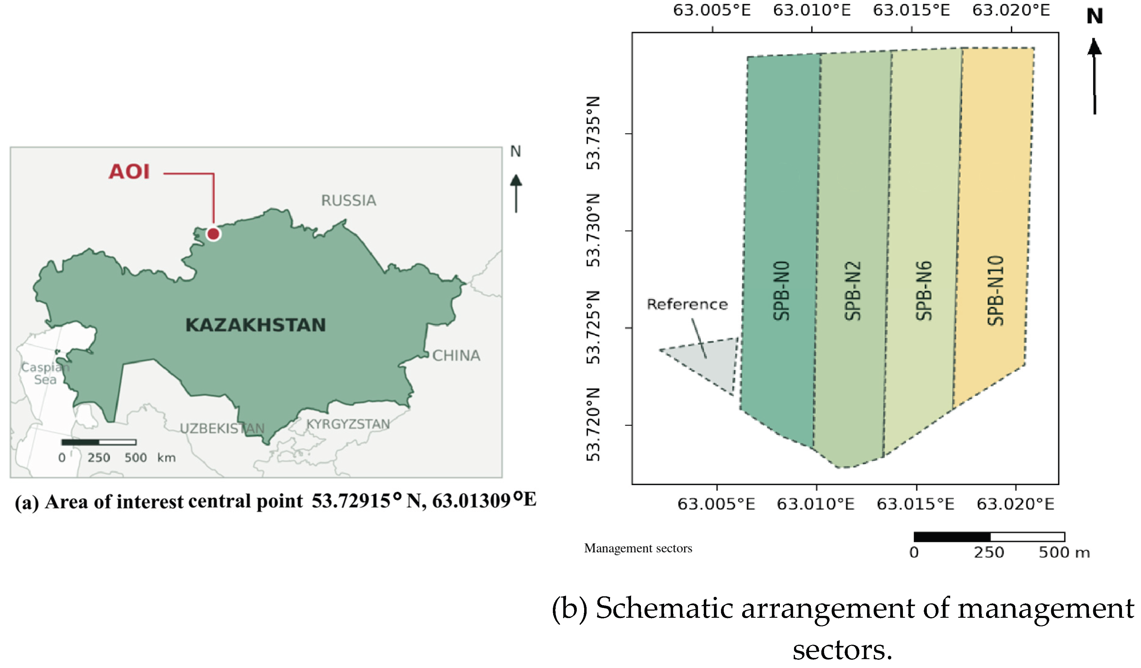
Figure 7.
Crop characteristics and grain quality by sector. Cell numbers indicate measurements, and color denotes the z-score of each characteristic across the five sectors. Plant height and thousand-kernel weight per crop sample are medians, while productive tillering, grain count per spike, and postharvest yield are means. Productive tillering is expressed as the number of ears per plant. Protein content describes the harvested grain sample from each sector.
Figure 7.
Crop characteristics and grain quality by sector. Cell numbers indicate measurements, and color denotes the z-score of each characteristic across the five sectors. Plant height and thousand-kernel weight per crop sample are medians, while productive tillering, grain count per spike, and postharvest yield are means. Productive tillering is expressed as the number of ears per plant. Protein content describes the harvested grain sample from each sector.
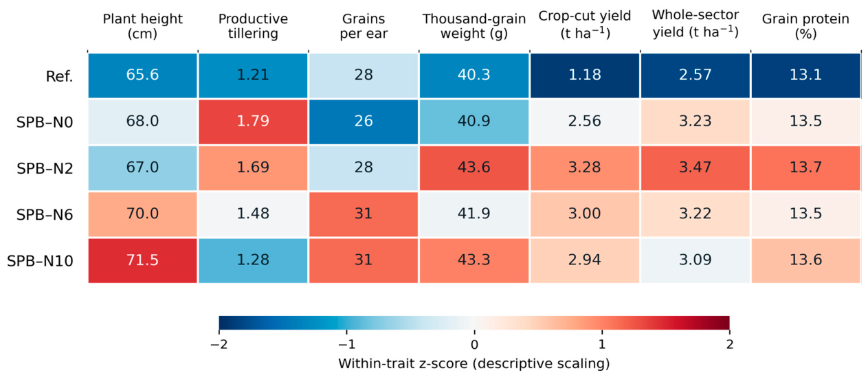
Figure 8.
Soil chemistry for June 8, July 5, and September 30, 2026: (a) nitrate nitrogen, (b) P2O5, (c) K2O, (d) sulfur, (e) salt extract pH, and (f) humus. Each point represents one composite sample for each sector and date. Lines connect successive surveys.
Figure 8.
Soil chemistry for June 8, July 5, and September 30, 2026: (a) nitrate nitrogen, (b) P2O5, (c) K2O, (d) sulfur, (e) salt extract pH, and (f) humus. Each point represents one composite sample for each sector and date. Lines connect successive surveys.
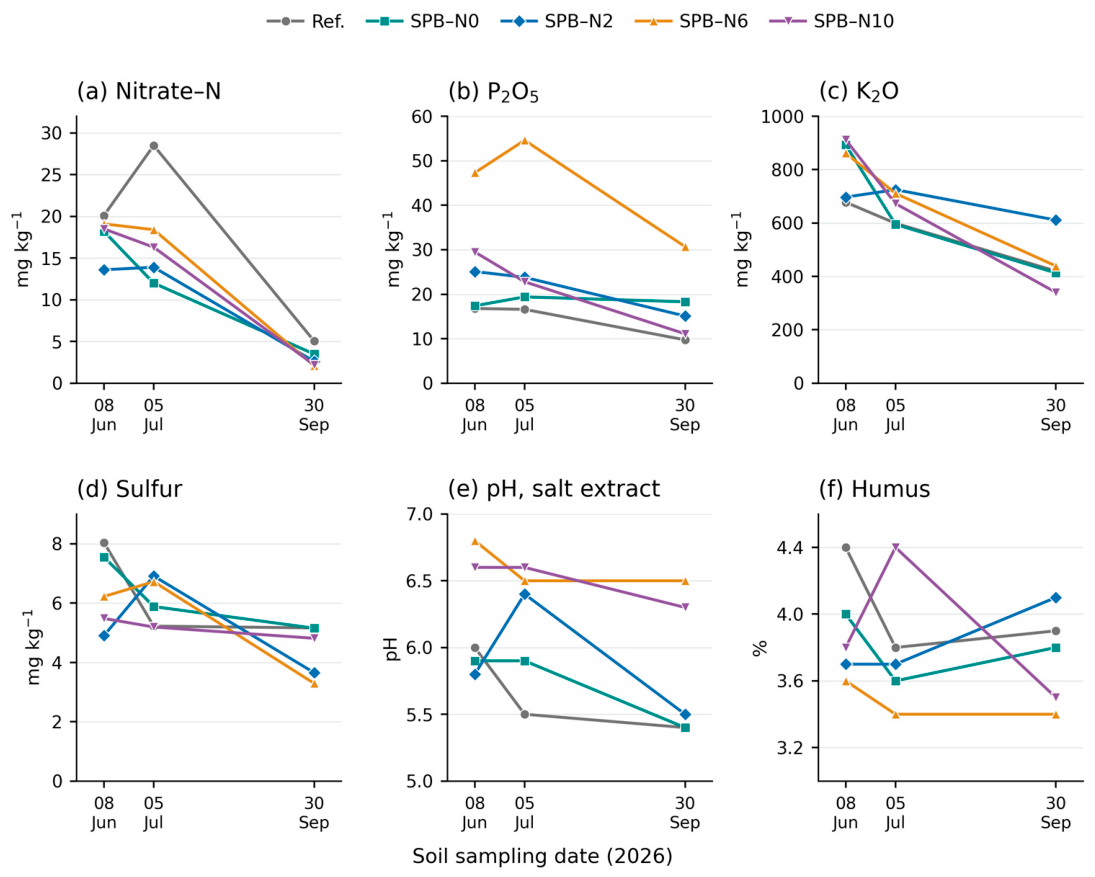
Table 1.
Components of the five management packs.
| Sector | Mineral nitrogen kg N ha−1 |
Powder before sowing kg ha−1 |
Powder at sowing kg ha−1 |
Liquid first application L ha−1 |
Liquid product for second use, l ha−1 |
Herbicide % full program |
|---|---|---|---|---|---|---|
| Link | 20 | 0 | 0 | 0 | 0 | 100 |
| SPB-N0 | 0 | 12 | 3 | 6 | 12 | 30 |
| SPB-N2 | 2 | 12 | 3 | 6 | 12 | 30 |
| SPB-N6 | 6 | 12 | 3 | 4 | 8 | 50 |
| SPB-N10 | 10 | 12 | 3 | 4 | 8 | 50 |
SPB stands for SoilPoint soil stimulant. The powder was applied before and during sowing. Liquid SPB was applied sequentially in July and August. Mineral nitrogen refers to elemental nitrogen applied as ammonium nitrate. The plant protection program in August was uniform across all sectors.
Table 2.
Sampling scheme, seasonal coverage and purpose of analysis.
| Data | Sampling plan and timing | Analysis |
|---|---|---|
| Sector Harvest | Five Sectors of Management, September 25 – October 1 | Profitability and relative industry differences |
| Sections and characteristics of agricultural crops | Five sections of 0.25 m2 per sector, 4–5 tillering/grain mass samples, 45–59 plant observations per sector. | Yield after cutting, tillering, height and ear/grain characteristics. |
| Flags | 20 sheets each in the SPB-N0 catalogue and in the reference catalogue, July 30. | Leaf area |
| Grain quality | One sample of collected grain per sector. | Protein, gluten, specific gravity and mass of grain |
| Chemical composition of the soil | One summary indicator for each sector for June 8, July 5 and September 30, 15 samples. | Seasonal changes in nutrient concentrations, pH and humus. |
| Soil moisture | Four probes x six depths x 92 dates, May 22 – August 21 | Average profile values, depth trajectories and seasonal decline. |
| NDVI | 12 observations using the Sentinel-2 satellite: three before sowing and nine after. | Average greenness of the sector and spatial structure |
| Precipitation | 92 daily indicators, the station is located 8.9 km southwest of the field center. | Precipitation timing and response to humidity signals |
Observations describe the complementary aspects of the crop-soil system. Sector-wide yield is the primary production indicator, while crop samples characterize yield components and grain quality. Repeated soil surveys and sensor-based telemetry describe the seasonal dynamics of chemical composition and moisture, while the NDVI index and hypsometry allow these observations to be placed in their spatial context.
Table 3.
Summary data on yield and harvest for the entire sector.
| Sector | Harvested area ha |
Yield across the sector, t ha−1 |
Mean cut yield ± standard deviation t ha−1 |
Slices n |
Reduction minus sector percentage |
|---|---|---|---|---|---|
| Link | 6.95 | 2.57 | 1.18 ± 0.32 | 5 | -54.1 |
| SPB-N0 | 43.66 | 3.23 | 2.56 ± 0.71 | 5 | -20.7 |
| SPB-N2 | 50.39 | 3.47 | 3.28 ± 0.63 | 5 | -5.5 |
| SPB-N6 | 42.35 | 3.22 | 3.00 ± 1.05 | 5 | -6.8 |
| SPB-N10 | 53.80 | 3.09 | 2.94 ± 0.35 | 5 | -4.9 |
Disclaimer/Publisher’s Note: The statements, opinions and data contained in all publications are solely those of the individual author(s) and contributor(s) and not of MDPI and/or the editor(s). MDPI and/or the editor(s) disclaim responsibility for any injury to people or property resulting from any ideas, methods, instructions or products referred to in the content. |
© 2026 by the authors. Licensee MDPI, Basel, Switzerland. This article is an open access article distributed under the terms and conditions of the Creative Commons Attribution (CC BY) license (http://creativecommons.org/licenses/by/4.0/).
Copyright: This open access article is published under a Creative Commons CC BY 4.0 license, which permit the free download, distribution, and reuse, provided that the author and preprint are cited in any reuse.