

Submitted:
01 October 2026
Posted:
04 October 2026
You are already at the latest version
Abstract
In this article we solve the diffusion-advection-reaction model problem with Robin boundary conditions in an open bounded domain Ω∈Rn, with n=1,2,3. For the discretization, we use the mixed-hybrid finite element method of lowest order on a simplicial partition of Ω¯. To prevent the occurrence of spurious unphysical oscillations we numerically evaluate the local bilinear form with a quadrature that is equivalent to introducing an optimal amount of artificial diffusion on each edge of the simplex. The resulting scheme is monotone and flux-conservative and is able to compute accurate solutions even with a corse mesh. The robustness and accuracy of the method is demonstrated on examples in Rn, n=1,2,3, characterized by the presence of steep boundary and internal layers.
Keywords:
finite elements
; mixed-hybrid
; monotonicity
; stabilization
; conservation
1. Introduction
Partial differential models of diffusion-advection-reaction (DAR) type are a relevant member of the family of second order elliptic equations because of their ubiquity in computatonal sciences. For example, systems of nonlinearly coupled DAR equations are frequently used to describe the spatio-temporal dynamics of cellular organisms [1] or charge density of electrons and holes in a semiconductor device [2]. Limiting our focus on the stationary case, DAR models are characterized by two important features:
- (F.1)
- conservation;
- (F.2)
- monotonicity.
To address (F.1), we introduce an arbitrary bounded volume in with boundary on which an outward unit normal vector is defined. We use the symbol u to represent the solution of the DAR model, for example, a concentration, and introduce the vector field and the scalar function , both depending on u, which represent a mathematical model of the motion of u across and the net production of u inside , respectively.
Definition 1 (Conservation of u)
If , we say that U is conserved, i.e., the amount of u that enters the volume exactly equals the quantity of u that leaves the volume. If , we say that the amount of u that leaves the volume is larger than the amount of u that enters the volume because of production of u inside the volume. If , we say that the amount of u that leaves the volume is smaller than the amount of u that enters the volume because of consumption of u inside the volume.
Definition 2 (Conservation of )
Let denote the approximate solution of the DAR model computed by a numerical scheme and depending by the discretization parameter h. The scheme is said to beconservativeif it satisfies (1a) at the discrete level, namely
where and denote the approximations of and , respectively, both depending on and h.
To address (F.2), we give the following definition.
Definition 3 (Monotonicity)
Assume that under suitable conditions on the coefficients of the model the solution u satisfies
Then, we say that the DAR model ismonotone.
Condition (2a) expresses the physical fact that a concentration of a chemical species or electric charge density cannot become negative. A natural request is that also the numerical scheme for the approximation of the solution of the DAR model is monotone. For this, we give the following definition.
Definition 4 (Monotonicity of the scheme)
Let us assume that there exists a value such that, for all , we have
If is finite, we say that the scheme isconditionally monotone, otherwise, if , we say that the scheme isunconditionally monotone(or simply,monotone).
Conditional and unconditional monotonicity are the counterpart of conditional and unconditional absolute stability of a numerical scheme for the Cauchy problem (see [4, Chapter 11]). Conditional monotonicity is due to the fact that the advective and/or reactive term of the DAR model dominates in magnitude over the diffusive term. In such a circumstance, the maximum permitted value of the mesh size may become extremely small with, at least, two negative consequences on the process of numerically solving the discrete DAR equation. The first consequence is that the number of degrees of freedom of is inversely proportional to , so that the number of flops (floating-point operations) to solve the linear algebraic system scales unfavorably with (as if a direct solver is adopted). The second consequence is that the condition number of the matrix of the system grows as , resulting into a significant deterioration of the solution quality and, if an iterative method is used, of the convergence rate. For these two reasons, ensuring the property of unconditional monotonicity of the numerical scheme is of paramount importance for an affordable, stable and accurate approximation of the solution of a DAR equation.
In this article we illustrate a conservative and monotone scheme for the numerical approximation of the stationary DAR model in a polyhedral domain , , subject to Robin boundary conditions. The scheme is a stabilized mixed-hybrid finite element (MHFE) method of lowest order (see [5]), whose output is a piecewise constant vector-valued function and a piecewise linear continuous scalar-valued function , that approximate the flux density and concentration u on a nonuniform partition of into simplices K of maximum diameter h.
The first step of the construction of the method follows [6] and consists of a change of dependent variable that transforms, for each , the non-symmetric DAR differential operator into a symmetric DR differential operator with an exponentially varying diffusion coefficient. The second step of the construction consists of using a quadrature formula to approximate the local bilinear form into a sum of contributions over the edges of the simplex K. This formula can be applied in all dimensions , and , and gives rise to a decomposition of into its tangential components on each edge of K that coincide with the Scharfetter-Gummel representation of the flux density in terms of the nodal values of on the edge (see [7]). This decomposition of on the edges of K resembles the "edge conditions" used to define the divergence-free upwinding method proposed in [8]. The third step of the construction consists of assembling the local stiffness matrix of the stabilized MHFE method into a global stiffness matrix which can be proved to be an M-matrix under suitable geometrical constraints on the partition (see [9, Lemma 2.1]). This algebraic property implies that the hybrid variable computed by the stabilized MHFE method satisfies (4) for all (unconditional monotonicity).
The remainder of the article is organized as follows. Section 2 describes the differential model. Section 3 illustrates the change of dependent variable that locally transforms the DAR equation into a DR equation with an exponentially varying diffusion coefficient. Section 4 describes the construction of the MHFE method and shows that it is conservative in the sense of Definition 2. Section 5 illustrates the matrix form of the scheme whereas Section 6 describes how to stabilize the MHFE method against advective and/or reactive dominating conditions. Stability and error analysis of the MHFE method are conducted in Section 7 whereas Section 8 describes how to recover the computed flux density by post-processing at the level of the single mesh element. Section 9 illustrates a series of simulation tests in all spatial dimensions to the purpose of validating the performance of the proposed method versus the nonstabilized formulation. Section 10 contains some summarizing conclusions and suggests possible research developments. Appendix A provides the numerical values of the model parameters in the simulation of the case study described in Section 9.2.
2. The Differential Model
Let denote an open polyhedral domain whose boundary is the surface on which an outward normal unit vector is defined. A point P belonging to is identified by its coordinates with respect to a fixed system of reference. The following partial differential equation (PDE) is a diffusion-advection-reaction mathematical model (DAR):
The flux density (units: ) and concentration u (units: U) are the dependent variables whereas c (units: ), (units: ), (units: ) and D (units: ) are the model coefficients representing the consumption term, the production term, the advective field and the diffusion coefficient, respectively. The function D is strictly positive in while c and are nonnegative in . The coefficients , (units: ) and (units: ) are given functions on . If we need to have and the boundary condition (3c) becomes the Dirichlet condition . If and , the boundary condition (3c) becomes a Robin boundary condition for u, while if and , the boundary condition (3c) becomes a Neumann boundary condition for u. The vector-valued function is a given velocity field which gives rise to a passive drifting force on u. Molecular diffusion according to Fick’s law is instead associated with the diffusion coefficient D.
If and , system (3) is a diffusion model for u; if and , system (3) is a diffusion-reaction model for u; conversely, if and , system (3) is a diffusion-advection model for u. In what follows we assume that the DAR boundary value problem (BVP) admits a unique solution depending with continuity on the data.
3. Local Symmetrization of the DAR Model
Let denote a regular triangulation of the domain into simplices K characterized by a diameter and a baricenter , with (see [10, Chapter 3]).
Assumption 1.
From now on, we assume that and D are replaced by their values and for each .
Using Assumption 1 we can write
where is a positive arbitrary reference concentration (units: U) and is defined as
Let us introduce the function
Inverting (7), we have
which can be written as
upon introducing the new dependent variable . Replacing (8) into the definition of we obtain
having used (5) to compute . The new dependent variable is known as "Slotboom variable" because it was originally introduced in [11] by J. Slotboom and subsequently adopted in [6] to construct mixed finite element approximations of the continuity equations for electrons and holes in the drift-diffusion model for semiconductor devices, We see that the "Slotboom change of variable" (8) has the effect of transforming the DAR differential operator into a symmetric DR differential operator characterized by a modified diffusion coefficient whose range depends exponentially on the dimensionless potential . Inverting (9) to express as a function of u, the flux density can be written as
4. The MHFE Discretization of Lowest Order
To simplify the presentation of the method, we assume that for all , which means that the DAR model is supplied with homogeneous Dirichlet boundary conditions. We define the set of the indices of all vertices of and we set . The set is divided into two subsets, namely, the set of the vertices belonging to the interior of , and the set of the vertices belonging to the boundary . We set and , with .
Let us introduce the functional spaces where to seek the flux density and concentration u, respectively:
Correspondingly, the finite dimensional spaces where to seek the approximations and computed by the MHFE method of lowest order are defined as:
The MHFE approximation of lowest order of the boundary value problem (3) reads:
Find and such that:
Let denote a vertex of belonging to the interior of , . We associate with the set constituted by the union of the simplexes sharing as a common vertex (see Figure 1 for a graphical representation of in the case ). We indicate by the basis function spanning the vector space that is linear on each simplex , and is such that and for all , . Based on this definition, the set is the support of (also referred to as the "patch" associated with ). The following result shows that the MHFE method is conservative in the sense of Definition 2.
Theorem 1
(Conservation of the MHFE method). The MHFE method satisfies (1b) by setting , and , respectively.
Proof.
The result immediately follows by taking in (12b) and using integration by parts in the first integral on the left hand side. □
Remark 1
(Conservation in 2D). In the case , the conservation property expressed by Theorem 1 corresponds to stating that the weighted sum of the jump of the normal flux density across the edges belonging to balances the net production over the support. This observation generalizes the considerations developed in [8] to support the stability of a novel divergence-free upwinding finite element approximation of the DAR equation in the case where .
Using the fact that is constant for each element K, denoted henceforth , and that over each element K and is equal to zero elsewhere, equation (12a) can be solved independently for each mesh element to obtain
from which we get
The quantity
is the harmonic average of over the n-dimensional simplex , having indicated by the n-dimensional volume of K (see [12] for the analysis of the role of the harmonic average in the numerical approximation of second-order ellliptic problems). Replacing the expression (13) in (12b), we obtain the final form of the MHFE formulation of lowest order in terms of the sole hybrid variable :
Find such that
where:
Assertion 1
(Well-posedness). We assume henceforth that the discrete problem (15a) is well posed, i.e., it admits a unique solution which depends with continuity on the model data.
5. Matrix Form of the MHFE Method
As it is customary in the context of the finite element methodology (see [13]), we introduce the local bilinear form composed of a diffusion-advection contribution and a reaction contribution
and the local linear functional , , defined as:
In all the above integrals, we denote by , , the linear function such that and for , with . Associated with the bilinear and linear forms in (17) we introduce the local diffusion-advection and reaction matrices of size :
and the local load vectors of size (column vectors):
After looping over the mesh elements to assemble the local stiffness matrix and load vector into the corresponding global matrix and right-hand side, and enforcing the boundary conditions, we obtain the following linear system
which represents the algebraic counterpart of Equation (15a).
Assertion 2 (Well-posedness of (20) Analogous to Assertion 1, we assume henceforth that the linear system (20) admits a unique solution .
6. Stabilization Via Numerical Quadrature
To implement in a computer code the bilinear forms and the linear functionals defined in (18) and (19), we make use of specific approximations and quadrature formulas. Let us start with the bilinear form (17a) that accounts for the diffusion and advection terms in the DAR model, and replace the function in (13) with its -interpolant over the element K. By doing this, the local approximate flux density becomes
Let us examine the expression (21) in the one-dimensional (1D) case (. Set with and indicate by , the nodal values of the dimensionless potential, with , so that , with . The harmonic average of the function is
where for , such that , represents the inverse of the Bernoulli function of . Inserting (22) in (21), in the case , we obtain
having used the property . The expression (23) coincides with the Scharfetter-Gummel (SG) formula originally derived in [7] and subsequently analyzed in [14,15]. Because of its second-order accuracy and numerical stability, and the automatic "upwind" weighting of the nodal values and , the one-dimensional SG formula (23) is universally employed in the simulation packages of the drift-diffusion model of semiconductor devices in multiple spatial dimensons (see [16,17]).
Motivated by the connection between the MHFE formulation and the SG method in the 1D case, we now address how to use the SG formula to compute the entries of the local matrix in the case . With this aim, we recall the following result proved in [18] and [9].
Lemma 1.
Let be a given constant vector in . Let also denote the edge with vertices and , length , and define on e a tangent vector directed from to . Then, we have
having set and , and where for any .
For any vertex of K, we denote by the set of the vertices of K that are adjacent to , . For example, taking , in the case we have , in the case we have , while if we have . The other expressions of the adjaciencies for can be determined cyclically. Using the definition of and , relation (24) becomes
where
and is the tangential component of along the edge directed from vertex to vertex , with length and tangent unit vector .
Assertion 3.
Let and denote the local stiffness matrix accounting for the diffusive and advective contributions and the column vector of size containing the nodal values of at the vertices of K, respectively. Let us also set . We approximate the matrix-vector product representation of (25) by means of the following quadrature formula
where:
with , .
Remark 2.
We complete the characterization of the MHFE method of lowest order by applying the n-dimensional trapezoidal quadrature to compute the entries of the local reaction matrix and load vector, obtaining:
The stabilized MHFE method of lowest order for the discretization of the DAR problem (3) reads:
Find such that
where:
The linear algebraic system of size associated with (30a) is
where is the global stiffness matrix of size whereas and are the solution vector and global load vector, both of size , respectively.
7. Stability and Error Analysis
In this section we leverage the theoretical analysis conducted in previous works to characterize the stability and convergence of the MHFEM illustrated in Section 6.
Theorem 2
(Stability). Let us assume that c and are given nonnegative functions in Ω. Let us also assume that the following geometrical constraint is satisfied for each edge
Then, the global stiffness matrix is an M-matrix, , and the stabilized MHFE method of lowest order is monotone.
Proof.
See the proof of Lemma 3.2 in [9] □
Remark 4.
Theorem 3
(Convergence). Assume that the solution pair of the DAR problem (3) is such that and , respectively. Then, there exists a positive constant C independent of h such that the following optimal error estimate holds
with and denoting the norm in the spaces V and Q defined in (11), respectively.
8. Post-Processing to Evaluate
Once system (31) is solved, we need to post-process the available nodal values of to determine the approximate flux density . A possible approach is suggested in [22], where the flux density inside the element is expressed as a function of the tangential flux density along each edge connecting vertices and , , with orientation from to , using the following interpolation formula
where
is the circulation of along the edge , with bnij, bp12, and being defined as in (27). In the reconstruction formula (34a), denotes the unit tangent vector along the edge directed from vertex to vertex , and the vector-valued functions , also known as Whitney elements (or "edge elements", see [23]), are defined as follows
9. Numerical Experiments in
In this section we conduct a series of numerical tests to validate the computational performance of the MHFE method in its nonstabilized and stabilized versions, by solving the DAR model problem in 1D, 2D and 3D geometries. In all considered cases, model coefficients are selected in such a way that the solution u exhibits the presence of steep internal and/or boundary layers whose accurate resolution would require, at least locally, the adoption of an extremely small mesh size. The main scope of the simulations is to demonstrate the ability of the stabilized MHFE to compute a solution pair with remarkable accuracy even on a coarse-sized mesh without being affected by spurious unphysical oscillations as it happens with the nonstabilized version of the scheme. The post-processing formula (34) is implemented in the codings to solve the DAR model in all spatial dimensions . All computations are performed using the Matlab scientific environment [24] on a HP laptop mounting an Intel Core i7-10510U processor at 1.80GHz.
9.1. The Case
In this section we study the DAR model problem (3) in the domain . The values of the parameters are: , , and . A rather coarse uniform partition of 20 elements of size is used in the computations. The boundary conditions are of nonhomogeneous Dirichlet type, with values and . Figure 2 illustrates the solution and the associated flux density computed by the stabilized MHFE method (solid line, blue color) and non-stabilized MHFE method (solid line, black color). For comparison, the exact solution is superposed (solid line, magenta color). Results indicate that the stabilized formulation captures the essential behavior of u and j even on the coarse mesh utilized in the test. In particular, no spurious oscillations arise in the vicinity of , where a steep boundary layer appears in the graphical plot of u and, less markedly, of j. The same comment cannot be applied to the concentration computed by the non-stabilized formulation, which is affected by wiggles that violate the monotonicity of u, reflecting also on the reconstruction of the flux density which shows some over/undershoot with respect to the almost constant profile of the exact solution j.
9.2. The Case
In this section we study the stationary continuity equation for the hole concentration p (units: ) in a two-dimensional (2D) cross-section of a p-n diode according to the so-called "Drift-Diffusion" model of charge transport in semiconductor devices (see [2] and [25]). The mathematical model of the problem consists of the following stationary boundary value problem in conservation form:
where is the computational domain shown in Figure 3, whose boundary is split into two disjoint subsets, and , on which the nonhomogeneous Dirichlet boundary condition (35c) and the homogeneous Neumann boundary condition (35d) are enforced, respectively.
The quantity (units: C) is the electron charge, p is the concentration of holes (units: ), is the hole diffusion coefficient (units: ), is the hole electric mobility (units: ), related to by Einstein’s relation
with denoting the thermal voltage (units: V), and is the electric potential (units: V). The quantities and represent the hole lifetime (units: s) and hole equilibrium concentration (units: ), respectively, whereas the vector is the hole current density (units: ). The computational domain consists of a square whose side is equal to , and represents the 2D cross-section of a p-n junction diode which is the union of three subdomains: the neutral region , the annular junction region , and the neutral region , having indicated by R and the radial coordinates such that and . The neutral regions are characterized by the fact that in while in and in , where:
The quantities and are the externally applied voltages (units: V) at the electric contact and , respectively, while and are the so-called "built-in" potentials (units: V).
The junction region JCT is characterized by the fact that , , with (units: s) and (units: ) being given positive constants, and
Remark 5.
After dividing q out of both sides of the balance equation (35a), we see that system (35) can be regarded as a special instance of system (3) upon setting , , (which corresponds to ), and , with τ equal to in .
Let us assume that , which amounts to setting the electric contact to ground voltage. If is equal to , the device is working in the so-called "thermal equilibrium" condition which is characterized by a current density for all . If is equal to a positive voltage, the device is working in the so-called "forward bias" condition, and the magnitude of is large in all the computational domain. If is equal to a negative voltage, the device is working in the so-called "reverse bias" condition, and the magnitude of is considerably smaller than in forward bias conditions, being smaller in than in the JCT region. In all biasing conditions, the hole concentration p is monotone in the sense of Definition 3. We refer to [26] for a physical discussion of the electrical function of the diode and to [27] for an analytical mathematical treatment.
Simulations are conducted on a nonuniform triangulation made of 870 elements and 468 vertices, with . The externally applied voltage at is , corresponding to moderately high reverse bias conditions, while the values of all the physical model parameters are illustrated in Appendix A The reconstruction formula (34a) is used to determine the current density in the stabilized and non-stabilized case.
Figure 4 shows the spatial distribution of and computed by the stabilized MH method. We notice that is monotone and exhibits the physically expected behavior: holes move by diffusion in the neutral regions and , while they are drifted by the large electric field in the JCT region towards the electric contact . The presence of the steep internal layer is the result of the huge difference between the very small hole concentration in the JCT region (due to the consumption term) and the very large hole concentration in the neutral region . The streamlines of the hole current density confirm the physical picture described by the plot of the hole concentration. In particular, we notice see that the magnitude of is small in all the device (because of reverse biasing conditions), except locally in the annular region (where the electric field has a very high strength) and around the point where the so-called "current-crowding" effect occurs due to an abrupt change from nonhomogeneous Dirichlet boundary condition to homogeneous Neumann boundary condition (see [14,35c,35d]).
Figure 5 shows the spatial distribution of and of the streamlines of computed by the non-stabilized MH method. The hole approximate concentration is not monotone and exhibits significant oscillations between the values and . The unphysical behavior of the solution computed by the non-stabilzed method is confirmed by the quiver plot of which is affected by vortices throughout all the computational domain.
9.3. The Case
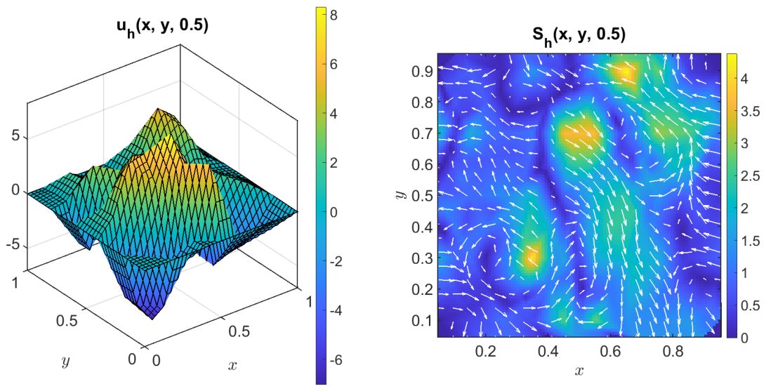
In this section we study the DAR model problem (3) in the domain subject to homogeneous Dirichlet boundary conditions. The values of the parameters are: , and , while advection is described by the counterclockwise rotating field . A rather coarse uniform partition of the domain is generated by subdividing each cube side into 5 intervals of length , resulting into a number of 216 vertices and 750 tetrahedra. The mathematical model under investigation can be regarded as the three-dimensional extension of the first numerical example studied in [9, Section 7]. Figure 6 illustrates the approximate solution and the streamlines of computed by the stabilized MHFEM, plotted in the plane at . Results indicate the rotation effect due to the advaction field, with the formation of sharp boundary layers along the sides and , without the onset of any spurious oscillations. In contrast to this, Figure 7 illustrates the approximate solution and the streamlines of computed by the non-stabilized MHFEM, plotted in the plane at . Results indicate the non-monotonicity of and the formation of local flow patterns which are totally inconsistent with the physically expected spatial distribution of the flux density vector field.
10. Conclusions and Perspectives
In this article we investigated the solution of the diffusion-advection-reaction boundary value problem. The emphasis was posed to the situation where advection and/or reaction dominate over diffusion because in this case the need of stabilization is particularly demanding in order to enforce the property of monotonicity on the discrete level, thereby preventig the occurrence of spurious unphysical oscillations in the solution computed by a numerical scheme. Conservation was also considered as an important property to be maintained on the discrete level by the numerical scheme chosen for approximation. Guided by these two principal objectives we illustrated the construction of a mixed hybrid finite element method of lowest order endowed with an edge-based stabilization which can be applied to any spatial dimension . The method was analyzed and numerically validated in several case studies characterized by different choices of the boundary conditions. Results demonstrated the attitude of the proposed stabilized method to compute stable and accurate solutions even on coarse domain partitions. This feature of the scheme makes it particularly attractive in the discretization of time-dependent multi-dimensional nonlinear systems of DAR equations for application in computational biology, in which the cost of a simulation is directly related to the repeated solution of linearized DAR boundary value problems required to advance over time levels.
Appendix A. Model Parameters in the Simulation of the P-N Diode
Table A1 contains the list of the values of model parameters that are used in the numerical simulation of the hole equation PDE system (35) in reverse bias conditions.

Table A1.
This table contains the list of the values of model parameters in the simulation od the 2D p-n junction diode. The values of and correspond to a doping concentration of in each neutral region.
Table A1.
This table contains the list of the values of model parameters in the simulation od the 2D p-n junction diode. The values of and correspond to a doping concentration of in each neutral region.
| Model parameter | Value | Units |
|---|---|---|
| L | m | |
| a | m | |
| m | ||
| m | ||
| V | ||
| 0 | V | |
| V | ||
| V | ||
| [] | ||
| [] | ||
| [s] | ||
| [] | ||
| [] | ||
| [] |
References
- Burzawa, L.; Li, L.; Wang, X.; Buganza-Tepole, A.; Umulis, D.M. Acceleration of PDE-Based Biological Simulation Through the Development of Neural Network Metamodels. Curr. Pathobiol. Rep. 2020, 8, 121–131. [Google Scholar] [CrossRef]
- Van Roosbroeck, W. Theory of the Flow of Electrons and Holes in Germanium and Other Semiconductors. j-BELL-SYST-TECH-J 1950, 29, 560–607. [Google Scholar] [CrossRef]
- Sacco, R.; Guidoboni, G.; Mauri, A.G. A Comprehensive Physically Based Approach to Modeling in Bioengineering and Life Sciences; Elsevier, Academic Press: Cambridge MA 02139, USA, 2019. [Google Scholar]
- Quarteroni, A.; Sacco, R.; Saleri, F. Numerical mathematics. In Texts in Applied Mathematics; Springer: Berlin, Heidelberg, New York, 2007; Vol. 37. [Google Scholar] [CrossRef]
- Boffi, D.; Brezzi, F.; Fortin, M. Mixed Finite Element Methods and Applications; Springer Series in Computational Mathematics; Springer Berlin Heidelberg, 2013; Vol. 44. [Google Scholar]
- Brezzi, F.; Marini, L.D.; Pietra, P. Two-Dimensional Exponential Fitting and Applications to Drift-Diffusion Models. SIAM J. Numer. Anal. 1989, 26, 1342–1355. [Google Scholar] [CrossRef]
- Scharfetter, D.; Gummel, H. Large-signal analysis of a silicon Read diode oscillator. IEEE Trans. Electron Devices 1969, 16, 64–77. [Google Scholar] [CrossRef]
- Bank, R.E.; Bürgler, J.F.; Fichtner, W.; Smith, R.K. Some upwinding techniques for finite element approximations of convection-diffusion equations. Numer. Math. 1990, 58, 185–202. [Google Scholar] [CrossRef]
- Xu, J.; Zikatanov, L.T. A monotone finite element scheme for convection-diffusion equations. Math. Comput. 1999, 68, 1429–1446. [Google Scholar] [CrossRef]
- Quarteroni, A.M.; Valli, A. Numerical Approximation of Partial Differential Equations, 1st ed 2nd printing ed.; Springer Publishing Company, Incorporated, 1994. [Google Scholar]
- Slotboom, J. Computer-aided two-dimensional analysis of bipolar transistors. IEEE Trans. Electron Devices 1973, 20, 669–679. [Google Scholar] [CrossRef]
- Babuška, I.; Osborn, J.E. Generalized Finite Element Methods: Their Performance and Their Relation to Mixed Methods. SIAM J. Numer. Anal. 1983, 20, 510–536. [Google Scholar] [CrossRef]
- Hughes, T.J.R. The Finite Element Method: Linear Static and Dynamic Finite Element Analysis; Dover Publications, 1987. [Google Scholar]
- Markowich, P.A. The Stationary Semiconductor Device Equations; Springer-Verlag: Wien, 1986. [Google Scholar]
- Sacco, R. Convergence of a second-order accurate Petrov–Galerkin scheme for convection–diffusion problems in semiconductors. Appl. Numer. Math. 1993, 11, 517–528. [Google Scholar] [CrossRef]
- Buturla, E.; Cottrell, P.; Grossman, B.M.; Salsburg, K.A. Finite-Element Analysis of Semiconductor Devices: The FIELDAY Program. IBM J. Res. Dev. 1981, 25, 218–231. [Google Scholar] [CrossRef]
- Synopsys; Inc. Sentaurus TCAD, Version Z-2023.03; Synopsys, Inc.: Mountain View, CA, USA, 2023. [Google Scholar]
- Bank, R.E.; Smith, R.K. The Finite Volume Scharfetter-Gummel method for steady convection diffusion equations. Comput. Vis. Sci. 1997, 1, 31–36. [Google Scholar] [CrossRef]
- Burgler, J.F.; Bank, R.E.; Fichtner, W.; Smith, R.K. A new discretization scheme for the semiconductor current continuity equations. Trans. Comp.-Aided Des. Integ. Cir. Sys. 2006, 8, 479–489. [Google Scholar] [CrossRef]
- Delaunay, B. Sur la sphè vide: A la mémoire de Georges Voronoï. Izv. Akad. Nauk SSSR Otd. Mat. I Estestv. Nauk 1934, 6, 793–800. [Google Scholar]
- Roberts, J.; Thomas, J.M. Mixed and hybrid methods. In Finite Element Methods (Part 1);Handbook of Numerical Analysis; Elsevier, 1991; Vol. 2, pp. 523–639. [Google Scholar] [CrossRef]
- Lazarov, R.D.; Zikatanov, L.T. An exponential fitting scheme for general convection-diffusion equations on tetrahedral meshes. arXiv 2012, arXiv:1211.0869. [Google Scholar]
- Bossavit, A. Whitney forms: a class of finite elements for three-dimensional computations in electromagnetism. IEE Proc. A (Physical Science, Measurement and Instrumentation, Management and Education) 1988, 135, 493–500. [Google Scholar] [CrossRef]
- Inc., T.M. MATLAB version: 9.10.0 (R2021a), 2021.
- Jerome, J.W. Analysis of charge transport; Springer-Verlag, 1996. [Google Scholar]
- Muller, R.S.; Kamins, T.I.; Chan, M. Device Electronics for Integrated Circuits, 3rd ed.; John Wiley & Sons: New York, 2003. [Google Scholar]
- Markowich, P.; Ringhofer, C.; Schmeiser, C. Semiconductor Equations; Springer Vienna, 1990. [Google Scholar]
- Murrmann, H.; Widmann, D. Current crowding on metal-semiconductor contacts. IEEE Trans. Electron Devices 1970, 17, 120–124. [Google Scholar] [CrossRef]
Figure 1.
Graphical representation of the set and of the basis function in the case . The red circle is the vertex . The function is defined also outside the support and its value is zero.
Figure 1.
Graphical representation of the set and of the basis function in the case . The red circle is the vertex . The function is defined also outside the support and its value is zero.
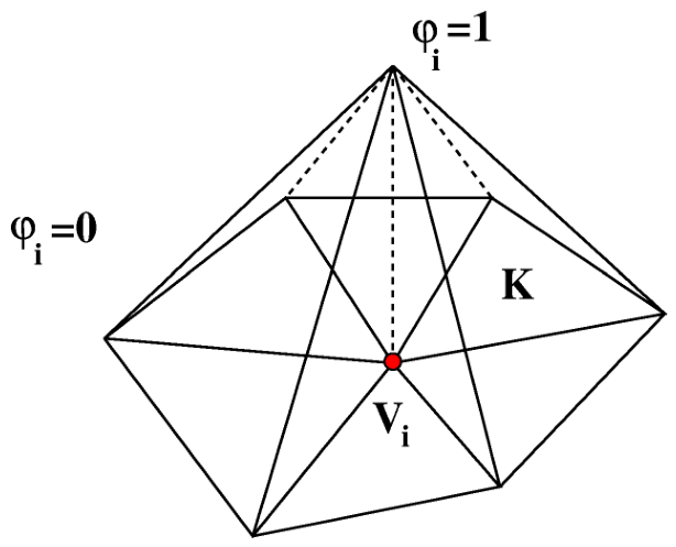
Figure 2.
Top: exact solution and approximate solutions computed by the stabilized method and non-stabilized method. Center: exact and approximate flux density computed by the stabilized method. Bottom: exact and approximate flux density computed by the non-stabilized method. In all panels, the exact solution is represented in magenta color, the approximate solution computed by the stabilized method is represented in blue color while the black color is used to represent the solution computed by the non-stabilized method.
Figure 2.
Top: exact solution and approximate solutions computed by the stabilized method and non-stabilized method. Center: exact and approximate flux density computed by the stabilized method. Bottom: exact and approximate flux density computed by the non-stabilized method. In all panels, the exact solution is represented in magenta color, the approximate solution computed by the stabilized method is represented in blue color while the black color is used to represent the solution computed by the non-stabilized method.
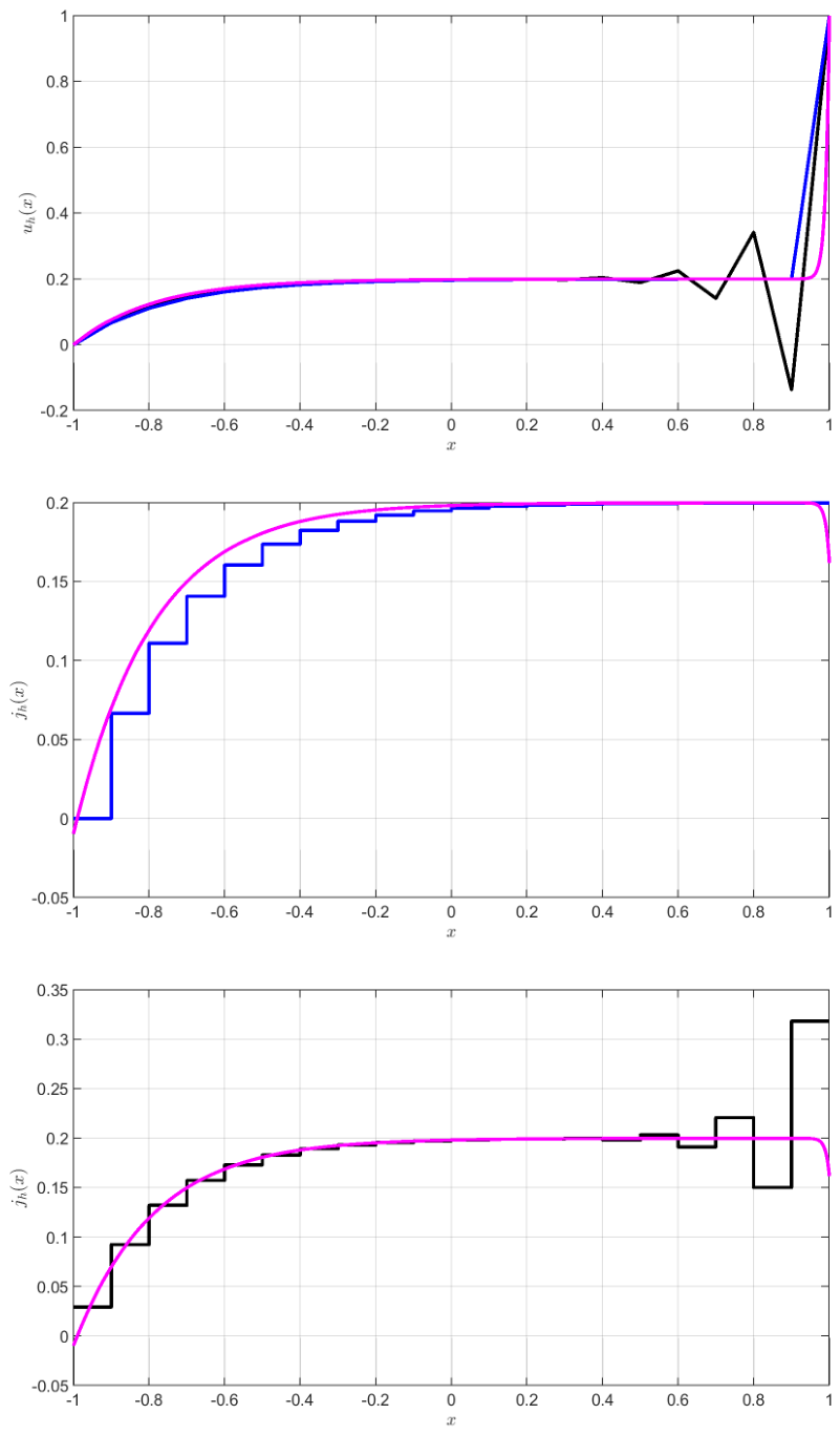
Figure 3.
Geometrical scheme of 2D p-n junction diode. The domain is the union of three regions: , JCT and . The thick segments in black color represent the portion of the boundary where Dirichlet conditions are enforced on u. On the remainder of the boundary homogeneous Neumann conditions are enforced on .
Figure 3.
Geometrical scheme of 2D p-n junction diode. The domain is the union of three regions: , JCT and . The thick segments in black color represent the portion of the boundary where Dirichlet conditions are enforced on u. On the remainder of the boundary homogeneous Neumann conditions are enforced on .
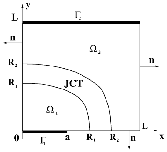
Figure 4.
Left panel: 3D plot of computed by the stabilized MHFEM. The solution is monotone, the minimum being and the maximum . Right panel: quiver plot of the streamlines of superposed to the colorbar of (units: ).
Figure 4.
Left panel: 3D plot of computed by the stabilized MHFEM. The solution is monotone, the minimum being and the maximum . Right panel: quiver plot of the streamlines of superposed to the colorbar of (units: ).
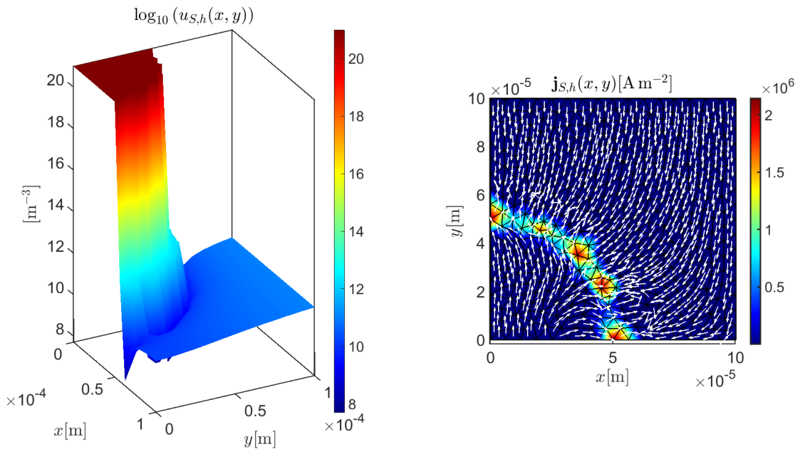
Figure 5.
Left panel: 3D plot of computed by the non-stabilized MHFEM. The solution is not monotone, the minimum being (negative!) and the maximum . Right panel: quiver plot of the streamlines of superposed to the colorbar of (units: ).
Figure 5.
Left panel: 3D plot of computed by the non-stabilized MHFEM. The solution is not monotone, the minimum being (negative!) and the maximum . Right panel: quiver plot of the streamlines of superposed to the colorbar of (units: ).
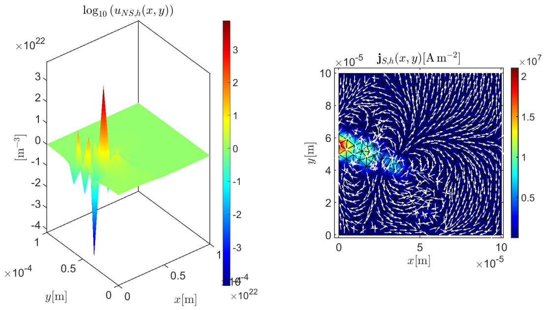
Figure 6.
Left panel: 3D plot of computed by the stabilized MHFEM. Right panel: quiver plot of the streamlines of superposed to the colorbar of . Quantities shown in the plots are evaluated at at , and .
Figure 6.
Left panel: 3D plot of computed by the stabilized MHFEM. Right panel: quiver plot of the streamlines of superposed to the colorbar of . Quantities shown in the plots are evaluated at at , and .
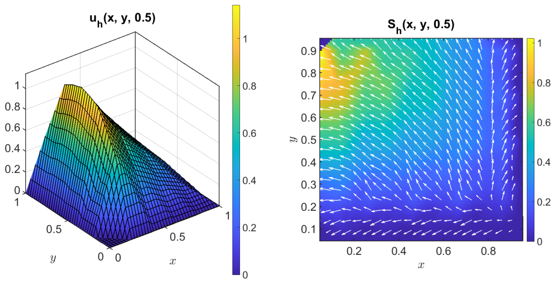
Figure 7.
Left panel: 3D plot of computed by the non-stabilized MHFEM. Right panel: quiver plot of the streamlines of superposed to the colorbar of . Quantities shown in the plots are evaluated at at , and .
Figure 7.
Left panel: 3D plot of computed by the non-stabilized MHFEM. Right panel: quiver plot of the streamlines of superposed to the colorbar of . Quantities shown in the plots are evaluated at at , and .
Disclaimer/Publisher’s Note: The statements, opinions and data contained in all publications are solely those of the individual author(s) and contributor(s) and not of MDPI and/or the editor(s). MDPI and/or the editor(s) disclaim responsibility for any injury to people or property resulting from any ideas, methods, instructions or products referred to in the content. |
© 2026 by the authors. Licensee MDPI, Basel, Switzerland. This article is an open access article distributed under the terms and conditions of the Creative Commons Attribution (CC BY) license (http://creativecommons.org/licenses/by/4.0/).
Copyright: This open access article is published under a Creative Commons CC BY 4.0 license, which permit the free download, distribution, and reuse, provided that the author and preprint are cited in any reuse.