
Submitted:
30 September 2026
Posted:
01 October 2026
You are already at the latest version
Abstract
Characterizing thin sandstone reservoirs remains challenging where strong lateral heterogeneity and limited seismic resolution make individual sand bodies difficult to distinguish. This study presents an integrated approach to reservoir characterization using 3D seismic and well-log data from a mature oilfield. Conventional seismic attributes, Highlight analysis, and spectral decomposition were combined with post-stack sparse-spike acoustic impedance inversion and AI-assisted high-resolution geostatistical inversion. Amplitude and Highlight attributes revealed consistent sandstone distribution patterns, while spectral decomposition identified distinct frequency responses at 55, 60 and 70 Hz across the investigated intervals. Conventional acoustic impedance inversion reproduced the main sandstone units but only partially resolved individual sand bodies approximately 2-8 m thick. The high-resolution geostatistical gamma-ray (GR) inversion sections revealed finer lithological variations than the conventional acoustic impedance inversion results. The upper intervals showed relatively continuous sandstone development, whereas the deeper intervals exhibited thinner sand bodies, greater siltstone development, and more pronounced lateral heterogeneity. These findings demonstrate the value of combining complementary seismic interpretation and inversion techniques to characterize complex sandstone reservoirs. The resulting geological interpretation provides a basis for further assessment of reservoir compartmentalization and potential interwell connectivity.
Keywords:
thin sandstone reservoirs
; seismic attributes
; spectral decomposition
; sparse-spike inversion
; geostatistical inversion
; artificial intelligence
; reservoir heterogeneity
1. Introduction
Accurate characterization of thin and laterally heterogeneous sandstone reservoirs remains a significant challenge in petroleum geoscience, particularly in mature oilfields with complex reservoir architecture. Identifying individual sandstone bodies and their spatial continuity is essential for understanding reservoir heterogeneity and evaluating potential interwell connectivity. However, conventional seismic interpretation is often constrained by limited vertical resolution, particularly where thin sandstone layers are interbedded with surrounding non-reservoir formations.
Seismic attribute analysis is widely applied to extract geological information from seismic data. Chopra and Marfurt [1] highlighted the importance of seismic attributes in structural and stratigraphic interpretation. Nevertheless, individual attributes may provide ambiguous results in heterogeneous reservoirs. Thin-bed characterization is further complicated by seismic tuning effects and limited seismic bandwidth, as demonstrated by Widess [2]. Spectral decomposition offers complementary information by analyzing seismic responses at individual frequencies. Partyka et al. [3] demonstrated its applications in reservoir characterization, while Castagna et al. [4] investigated frequency-dependent seismic anomalies using instantaneous spectral analysis.
Seismic inversion provides an additional approach for estimating subsurface rock properties and identifying lithological boundaries. Conventional post-stack acoustic impedance inversion, however, remains constrained by seismic bandwidth, wavelet estimation, and the reliability of the initial low-frequency model. Zhang and Castagna [5] investigated sparse-layer reflectivity inversion, highlighting the potential advantages of incorporating thin-layer reflectivity patterns. Geostatistical inversion further extends conventional approaches by integrating seismic observations, well-log information, and geological constraints. Bosch et al. [6] reviewed the application of statistical rock physics and geostatistics in seismic inversion, while Azevedo et al. [7] demonstrated the integration of well data into geostatistical inversion for facies estimation.
Recent advances in artificial intelligence have introduced additional opportunities for seismic inversion and reservoir characterization. Biswas et al. [8] investigated physics-guided convolutional neural networks for prestack and poststack inversion. Alfarraj and Alregib [9] developed a semi-supervised framework incorporating well-log information and geophysical constraints, while Das et al. [10] explored convolutional neural networks for seismic impedance inversion. These studies demonstrate the potential of combining data-driven approaches with conventional geophysical methods, although their reliability remains dependent on data quality, geological constraints, and appropriate validation.
Despite these advances, characterizing thin and discontinuous sandstone bodies remains challenging because seismic attributes, conventional inversion, and high-resolution geostatistical modelling provide different but complementary information. Integrating these techniques within a consistent workflow may improve the representation of complex reservoir architecture and reduce uncertainties associated with individual interpretation methods.
The reservoir investigated in this study is characterized by thin sandstone bodies, pronounced lateral lithological variability, and complex relationships between individual reservoir units. The investigation primarily focuses on three target sand groups: M-0-1-B, M-0-2-A, and M-0-2-B, while adjacent intervals are considered to evaluate the broader reservoir architecture.
Accordingly, this study applies an integrated workflow combining conventional seismic attributes, Highlight attribute analysis, spectral decomposition, post-stack sparse-spike acoustic impedance inversion, and AI-assisted high-resolution geostatistical inversion. Objectives are to characterize the spatial distribution and lateral continuity of the target sandstone intervals, to investigate their frequency-dependent seismic responses, to evaluate the limitations of conventional inversion in resolving thin sandstone bodies and to examine the additional lithological detail provided by high-resolution geostatistical inversion. The integrated interpretation aims to provide a more detailed geological representation of heterogeneous sandstone reservoirs.
2. Materials and Methods
2.1. Study Area and Dataset
The study was conducted in a mature oilfield characterized by a heterogeneous multilayer sandstone reservoir. The investigated reservoir system consists of thin sandstone bodies with pronounced lateral lithological variations and complex relationships between individual reservoir units. The analysis primarily focuses on three sandstone intervals: M-0-1-B, M-0-2-A, and M-0-2-B, while other relevant intervals were also considered to provide a more comprehensive understanding of the reservoir structure.
The dataset comprises three-dimensional (3D) post-stack seismic data and well-log measurements, including gamma-ray (GR), sonic (DT), density (RHOB), and resistivity logs. These data were used for seismic attribute analysis, well-to-seismic calibration, acoustic impedance inversion, and high-resolution reservoir characterization. The field name and precise geographical location are withheld due to confidentiality restrictions.
2.2. Conventional Seismic Attributes
Seismic attribute technology involves extracting useful hidden information from seismic data, including phase, frequency, amplitude, and other seismic parameters. By integrating seismic attributes with well data, variations in seismic responses are analyzed both vertically and laterally from different perspectives. This process establishes the relationship between seismic attributes and the geophysical characteristics of geological bodies, ultimately enabling the prediction of geological targets under similar geological conditions [1].
In this study, a total of 35 conventional seismic attributes, including amplitude-related and instantaneous attributes, were extracted for the three target sand groups: M-0-1-B, M-0-2-A, and M-0-2-B. Through multi-attribute comparative analysis, amplitude-related attributes were found to show the best agreement with well control and reservoir distribution.
2.3. Highlight Technology
Highlight is defined as the difference between peak amplitude and the amplitude in effective frequency band (Figure 1). In seismic data, the presence of sand bodies causes changes in frequency spectra. Compared with the structures that are not sand bodies, and sand bodies are anomalies on seismic spectra. These anomalies can be characterized by highlight attributes, so that highlight technology can effectively predict the distribution of sand bodies (Figure 2).
2.4. Spectral Decomposition
Spectral decomposition is post-stack data processing and interpretation. Starting from frequency domain, first scan and analyze the amplitude energy at different frequencies and then calculate attribute data while ignoring the mutual interference between frequency components in time domain. Without well data, spectral decomposition can provide higher resolution than in time domain under the same conditions. Spectral decomposition technology has more advantages than traditional seismic attributes in describing reservoir morphology and changing rules [3,4].
Spectral decomposition can continuously convert the sampling points on a seismic trace from time domain to frequency domain to obtain the spectrum information. Its core is to transfer seismic data to frequency domain to build tuning cube data through mathematical transform such as discrete Fourier transform or maximum entropy. Spectral decomposition makes full use of the change of the periodic notched spectrum of a thin layer with thickness, so it can not only qualitatively analyze reservoir, but also quantitatively calculate the reservoir thickness (Figure 3).
2.5. Sparse Spike Inversion
Sparse-spike inversion is one of the most widely used post-stack acoustic impedance inversion techniques. For the three target sand groups within Development Zone III of the Field X well block, a conventional post-stack sparse-spike seismic inversion workflow was applied in this study. Constrained by well-log data, the technique inverts seismic data to generate a P-wave acoustic impedance volume.
The inversion results effectively reveal acoustic impedance contrasts between reservoir rocks and surrounding formations, thereby facilitating the identification of the spatial distribution and lateral variations of sand bodies. In addition, the sparse-spike inversion results serve as a benchmark for evaluating and validating the subsequent AI-based high-resolution seismic inversion results.
2.6. Synthetic Seismogram Calibration and Wavelet Extraction
Based on the standardized well-log data, synthetic seismogram calibration and average wavelet extraction were subsequently carried out. First, reflection coefficient series were generated from the standardized sonic and density logs and convolved with Ricker wavelets of different dominant frequencies to produce synthetic seismograms. Through detailed correlation and matching with the seismic traces adjacent to each well, the time-depth relationship was refined, enabling accurate calibration of major seismic reflectors and target horizons [6]. Based on the multi-well calibration results, an average wavelet representative of the study area was extracted to provide consistent phase and frequency characteristics for the subsequent seismic inversion process.
The third development layer system in the well block is characterized by a typical “single sand body–single reservoir” (one sand, one reservoir) depositional model. The sand bodies are thin in individual thickness, exhibit strong lateral heterogeneity, and show complex connectivity between sand units. Conventional post-stack seismic inversion based on sparse-spike algorithms is constrained by the seismic bandwidth, making it difficult to reliably delineate the true boundaries of thin sand bodies and their internal property variations. As a result, the connectivity between injection and production wells remains poorly understood, and the direction of water-flood response is uncertain, thereby limiting the optimization of well pattern adjustment and remaining oil potential tapping.
In this study, AI-based high-precision inversion is applied to overcome the limitations of conventional inversion in resolving thin sand bodies. In practice, a high-resolution geostatistical inversion framework is adopted as the core inversion engine, as it can fully integrate high-frequency information from well logs and quantify uncertainty. However, this method is limited by low computational efficiency, reliance on manually defined variogram parameters, and the lack of automatic integration of multiple realizations. To address these issues, an artificial intelligence module is introduced to enhance the workflow, forming a hybrid framework of “geostatistical inversion + deep learning post-processing.” This approach preserves the geological reliability of geostatistical inversion while significantly improving both accuracy and computational efficiency through intelligent optimization [8,9,10].
The overall technical workflow of the AI-based high-precision seismic inversion consists of four main steps:
- High-resolution geostatistical inversion (modified geostatistical inversion): By decoupling the frequency components of broadband inversion results, this step integrates deterministic seismic inversion with geostatistical methods to achieve fine-scale prediction of thin reservoirs.
- AI-based automatic variogram fitting: Deep neural networks are employed to automatically learn optimal variogram parameters from well data and seismic attributes.
- Generation of multiple geostatistical realizations: Under AI-optimized parameters, hundreds of equiprobable acoustic impedance realizations are rapidly generated using geostatistical inversion.
AI-based multi-realization fusion and super-resolution reconstruction: A convolutional neural network is used to fuse multiple realizations into a single high-resolution acoustic impedance volume, while enhancing the delineation of thin sand-body boundaries.
3. Results
Amplitude attributes generally reflect variations in fluid content, lithology, reservoir porosity, formation formation thickness, and formation pressure. They are effective in identifying amplitude anomalies and stratigraphic features and are particularly useful for delineating fluvial channel systems.
As shown in Figure 4 and Figure 5, the amplitude attributes map of the interval from M-0-1-A to M-0-2-B are presented, where warm colors indicate the distribution of sand bodies. The M-0-1-A sand body is mainly developed in the central part of the study area and trends in a northwest–southeast (NW-SE) direction. The M-0-1-B and M-0-2-A sand bodies are characterized by extensive distribution and good continuity, occurring primarily in the central and southern parts of the study area. The M-0-2-B interval is relatively deeper, with poorer sand-body continuity, and is mainly distributed in the central and northern parts of the study area.
The distribution patterns revealed by the highlight volume attributes are generally consistent with those identified from the amplitude attributes.
The M-0-1-A sand body is mainly developed in the central part of the study area and exhibits a northwest-southeast (NW-SE) orientation. The M-0-1-B and M-0-2-A sand bodies are characterized by extensive areal distribution and good lateral continuity, occurring predominantly in the central and southern parts of the study area. The M-0-2-B interval is relatively deeper and exhibits poorer sand-body continuity. Due to stratigraphic pinch-out, sand bodies in the northern drilling area are only sporadically developed.
Using amplitude tuner to predict thin reservoir originates from Widess’s method of using seismic amplitude to quantitatively study reservoir thickness. For underground formation, the seismic reflection amplitude increases gradually with the increase of thickness. When the formation thickness increases to 1/4 wavelength, namely the tuning thickness, the amplitude of the reflected wave reaches the maximum value, and then the amplitude decreases gradually with the increase of the formation thickness. Based on this principle, thin layer tuning and interference effects are applied to analyze reservoir thickness and plane distribution by determining the tuning amplitude and tuning frequency on the tuning cube data and carry out qualitative and quantitative prediction of thin reservoirs. Without logging data, the resolution to thin reservoirs is higher than in time domain under the same conditions.
Figure 6 and Figure 7 present the spectral decomposition attribute maps of the interval from M-0-1-A to M-0-2-B, where warm colors indicate the distribution of sand bodies.
The distribution characteristics of the M-0-1-A sand body are clearly displayed on the 70 Hz frequency slice, which highlights the development of thin sand bodies in the central and northern parts of the study area. The M-0-1-B sand body shows a good correspondence with the 55 Hz frequency slice, revealing extensive and laterally continuous sand-body development in the central and southern portions of the study area.
Both the M-0-2-A and M-0-2-B sand bodies can be effectively identified on the 60 Hz frequency slice. Compared with the overlying intervals, M-0-2-B occurs at a greater burial depth and exhibits poorer lateral continuity of sand bodies.
Environmental corrections and log standardization were completed for all wells in the Fields X well block. The distribution histograms of the standardized sonic logs from selected wells in the study area show that the sonic log responses have been normalized to a consistent range and are now comparable on the same scale. This indicates that the log data satisfy the quality requirements for the seismic inversion workflow (Figure 8).
Synthetic seismogram generation and well-to-seismic calibration were completed for all 94 wells in the Fields X well block. By quantitatively evaluating the correlation coefficients and waveform matching quality between the synthetic seismograms and nearby seismic traces, 54 wells with high calibration quality and reliable time-depth relationships were selected. These wells were subsequently used for average wavelet extraction and seismic inversion, ensuring the accuracy, reliability, and representativeness of the inversion input data (Figure 9, Figure 10 and Figure 11).
Based on well-log standardization, synthetic seismogram calibration, and average wavelet extraction, a low-frequency model was further constructed. First, standardized P-wave impedance logs were extracted from 96 selected wells with high-quality calibration results. Combined with seismic interpretation horizon constraints, a distance-weighted interpolation method was applied to build a regional low-frequency background model. This model effectively compensates for the missing low-frequency components in seismic data, providing reliable initial constraints for model-based seismic inversion and improving the resolution and accuracy of reservoir characterization.
The previously interpreted horizons of M-0-1-A, M-0-1-B, M-0-2-A, M-0-2-B, M-0-3-A, and M-0-3-B were used as control surfaces to establish a geological framework model. The consistency between well-based acoustic impedance and interpolated impedance at model nodes was repeatedly checked. Wells with abnormal responses were removed, and the model was iteratively updated to improve well-to-model matching. As a result, the lateral variations became more geologically reasonable and consistent with sedimentary depositional patterns. Ultimately, a final acoustic impedance low-frequency model was established (Figure 12).
Figure 13, Figure 14 and Figure 15 show the acoustic impedance inversion sections across the southern, central, and northern parts of the study area, respectively. Petrophysical analysis indicates that sandstone exhibits relatively high acoustic impedance characteristics; in the inversion sections, warm colors (yellow to red) correspond to sandstone distribution.
The inversion profiles clearly show the development of sandstone within the M-0-1-A to M-0-2-A intervals, with good lateral continuity. In deeper formations, cooler colors (blue to green) indicate relatively higher shale content, and the lateral continuity of sandstone bodies becomes poorer.
In the vertical direction, the acoustic impedance inversion is derived from conventional seismic data volumes; therefore, thin sand bodies at well locations (2-8 m) are only partially resolved, resulting in limited vertical resolution.
In addition, in some areas such as the lower part of well W-68 shown in Figure 15-abnormally high impedance values appear at the base of the section due to the influence of high-velocity, high-density basement metamorphic rocks (Paleozoic, Pz). This anomaly affects the accuracy of sandstone reservoir prediction in the inversion results.
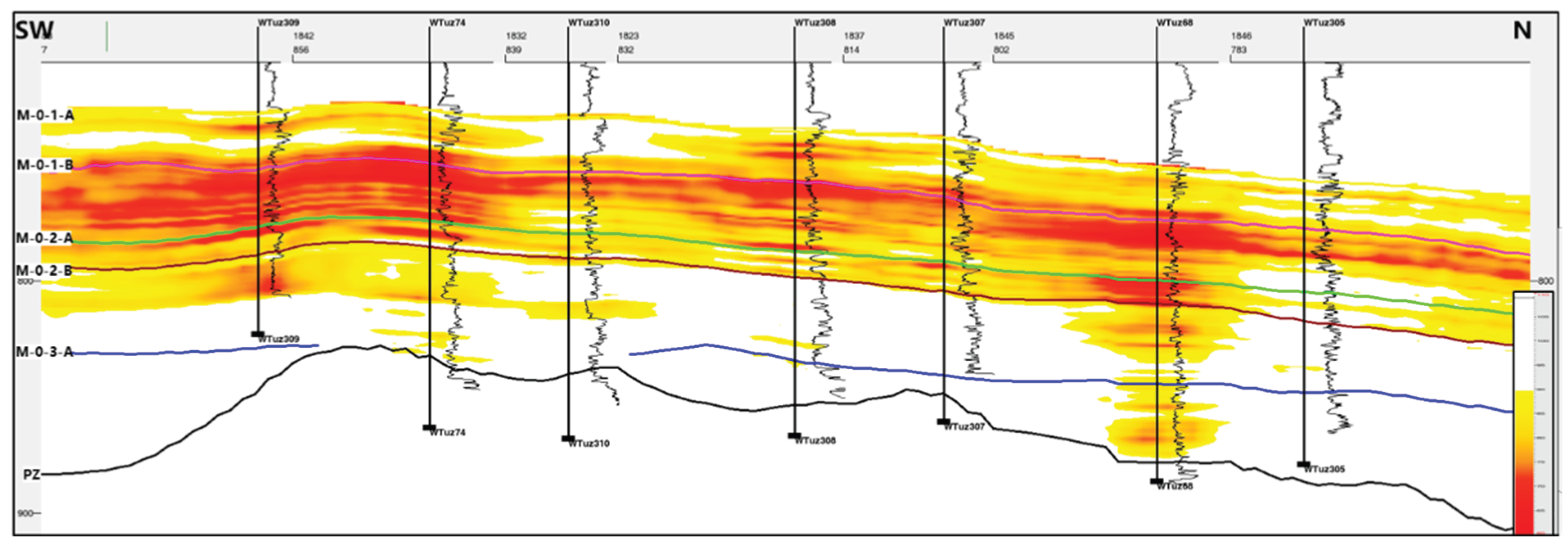
Figure 16, Figure 17 and Figure 18 present the GR (Gamma Ray) inversion sections across the southern, central, and northern parts of the study area, respectively. Based on single-well sandstone interpretation and petrophysical analysis, red colors in the inversion sections represent clastic sandstone and coarse-grained sandstone, while orange colors indicate the distribution of sandstone and siltstone.
The inversion profiles show well-developed coarse-grained sandstone within the M-0-1-A, M-0-1-B, and M-0-2-A intervals, with high lithological consistency between wells, relatively large thickness, and good lateral continuity.
Influenced by depositional environments, the deeper M-0-2-B and M-0-3-A intervals are characterized by relatively more siltstone development. These intervals exhibit rapid lateral lithological variations between wells, with thinner sandstone bodies and poorer lateral continuity observed in the inversion sections.
Compared with conventional acoustic impedance inversion results, the high-precision geostatistical GR inversion significantly improves both lateral and vertical resolution. Given the “one sand body, one reservoir” characteristics of the study area, these results provide a strong basis for further analysis of sand-body scale, connectivity, and injection-production relationship between well groups.
4. Discussion
The results of this study demonstrate the importance of the integrated use of various seismic attributes for characterizing thin-bedded and laterally heterogeneous sandstone reservoirs. Traditional amplitude attributes provided an initial understanding of the spatial distribution of the target sand bodies, while analysis of the Highlight attribute revealed distribution patterns that were generally consistent with these findings. The agreement between the results obtained using these independent attributes confirms the value of applying them in combination to identify key productive intervals.
Spectral decomposition provided additional information regarding the frequency-dependent seismic responses of individual sand bodies. The M-0-1-A interval was most clearly defined on the 70 Hz frequency slice, whereas M-0-1-B showed a more pronounced response on the 55 Hz slice. The M-0-2-A and M-0-2-B intervals were effectively identified at 60 Hz. These differences suggest that the target intervals exhibit distinct seismic responses linked to the seismic tuning effect, potentially driven by variations in reservoir thickness and acoustic properties.
The observed frequency dependence also indicates that using a single frequency slice may be insufficient to characterize all productive intervals. Consequently, combining traditional amplitude attributes, Highlight analysis, and spectral decomposition provides a more comprehensive interpretation of sand body distribution compared to using a single attribute.
Traditional sparse-spike inversion successfully reproduced the general acoustic impedance distribution and the main sand intervals within the study area. However, the inversion results revealed limitations in resolving individual thin sand bodies, particularly those with thicknesses of approximately 2–8 m.
This limitation is consistent with the insufficient vertical resolution of band-limited seismic data. Although sparse-spike inversion enables the recovery of acoustic impedance contrasts and the construction of a general geological model, closely spaced thin layers may remain unresolved or appear as a composite seismic response. Consequently, the apparent continuity of sand intervals on conventional inversion sections does not necessarily indicate the actual continuity of individual reservoir bodies.
Compared to traditional acoustic impedance inversion, high-resolution geostatistical GR inversion sections provided a more detailed depiction of lithological variations within the target intervals. The results indicate relatively continuous sandstone development in the M-0-1-A, M-0-1-B, and M-0-2-A intervals, whereas the deeper M-0-2-B and M-0-3-A intervals are characterized by pronounced lateral heterogeneity and reduced continuity of the sand bodies.
These observations are particularly relevant to the reservoir under study, which is characterized by a “single sand body-single reservoir” geological architecture. Under such geological conditions, identifying individual sand bodies and their lateral interrelationships is crucial for assessing reservoir compartmentalization and potential inter-well connectivity.
Integrated interpretation revealed differences in sandstone development and lateral continuity between the studied productive intervals. The relatively continuous sandstone distribution in the upper intervals contrasts with the more heterogeneous structure of the deeper-seated formations. These differences may be significant for assessing reservoir connectivity and identifying potentially isolated sand bodies.
5. Conclusions
This study investigated the characterization of thin and laterally heterogeneous sandstone reservoirs through an integrated workflow combining seismic attribute analysis, spectral decomposition, conventional sparse-spike inversion, and AI-assisted high-resolution geostatistical inversion.
Conventional amplitude attributes and Highlight analysis revealed generally consistent spatial distribution patterns of the investigated sandstone bodies. The M-0-1-A interval is predominantly developed in the central part of the study area, whereas M-0-1-B and M-0-2-A exhibit broader distribution and relatively good lateral continuity. In contrast, the deeper M-0-2-B interval shows a more discontinuous sandstone distribution.
Spectral decomposition provided additional information on the frequency-dependent responses of individual reservoir intervals. The M-0-1-A sandstone body was most clearly identified at 70 Hz, M-0-1-B at 55 Hz, and M-0-2-A and M-0-2-B at 60 Hz. These differences demonstrate the importance of selecting appropriate frequency components when interpreting thin sandstone reservoirs.
Conventional sparse-spike acoustic impedance inversion successfully reproduced the general distribution of the major sandstone intervals. However, individual thin sand bodies with thicknesses of approximately 2–8 m were only partially resolved, highlighting the limitations imposed by the vertical resolution of conventional seismic data.
Compared with conventional acoustic impedance inversion, high-resolution geostatistical GR inversion provided a more detailed representation of lithological variations within the investigated intervals. The resulting sections indicate relatively continuous sandstone development in M-0-1-A, M-0-1-B, and M-0-2-A, while M-0-2-B and M-0-3-A exhibit thinner sandstone bodies, increased siltstone development, and more pronounced lateral heterogeneity.
Overall, the integration of complementary seismic attributes and inversion techniques provided a more detailed interpretation of the reservoir architecture than conventional seismic inversion alone. The results highlight the importance of resolving individual sandstone bodies in reservoirs characterized by single sand-body reservoir architecture and provide a geological basis for further assessment of reservoir compartmentalization.
Author Contributions
Conceptualization, K.Z.; methodology, N.A.; software and investigation, I.M.; resources, C.L.; formal analysis and data curation, A.K.; visualization, J.I.; writing-original draft preparation, A.K.; writing-review and editing, J.I.; supervision, A.I.; project administration, K.Z. All authors have read and agreed to the published version of the manuscript.
Data Availability Statement
The data supporting the findings of this study are not publicly available due to confidentiality restrictions associated with proprietary seismic and well-log data provided by the field operator.
Acknowledgments
This research was carried out within the framework of the project «Study and development of new methods for optimizing the development of the Western Tuzkol field under conditions of strong heterogeneity and facies variability of reservoirs, as well as discontinuity of hydrocarbon accumulations (within contract area No. 4671)», state registration number 0126РКН0059.
Conflicts of Interest
The authors declare no conflicts of interest.
References
- Chopra, S.; Marfurt, K.J. Seismic attributes-A historical perspective. Geophysics 2005, 70, 3SO–28SO. [Google Scholar] [CrossRef]
- Widess, M.B. How thin is a thin bed? Geophysics 1973, 38, 1176–1180. [Google Scholar] [CrossRef]
- Partyka, G.; Gridley, J.; Lopez, J. Interpretational applications of spectral decomposition in reservoir characterization. Lead. Edge 1999, 18, 353–360. [Google Scholar] [CrossRef]
- Castagna, J.P.; Sun, S.; Siegfried, R.W. Instantaneous spectral analysis: Detection of low-frequency shadows associated with hydrocarbons. Lead. Edge 2003, 22, 120–127. [Google Scholar] [CrossRef]
- Zhang, R.; Castagna, J.P. Seismic sparse-layer reflectivity inversion using basis pursuit decomposition. Geophysics 2011, 76, R147–R158. [Google Scholar] [CrossRef]
- Bosch, M.; Mukerji, T.; Gonzalez, E.F. Seismic inversion for reservoir properties combining statistical rock physics and geostatistics: A review. Geophysics 2010, 75, 75A165–75A176. [Google Scholar] [CrossRef]
- Azevedo, L.; Nunes, R.; Soares, A.; Mundin, E.C.; Neto, G.S. Integration of well data into geostatistical seismic amplitude variation with angle inversion for facies estimation. Geophysics 2015, 80, M113–M128. [Google Scholar] [CrossRef]
- Biswas, R.; Sen, M.K.; Das, V.; Mukerji, T. Prestack and poststack inversion using a physics-guided convolutional neural network. Interpretation 2019, 7, SE161–SE174. [Google Scholar] [CrossRef]
- Alfarraj, M.; Alregib, G. Semi-supervised sequence modeling for elastic impedance inversion. Interpretation 2019, 7, SE237–SE249. [Google Scholar] [CrossRef]
- Das, V.; Pollack, A.; Wollner, U.; Mukerji, T. Convolutional neural network for seismic impedance inversion. Geophysics 2019, 84, R869–R880. [Google Scholar] [CrossRef]
Figure 1.
Schematic highlight attributes.
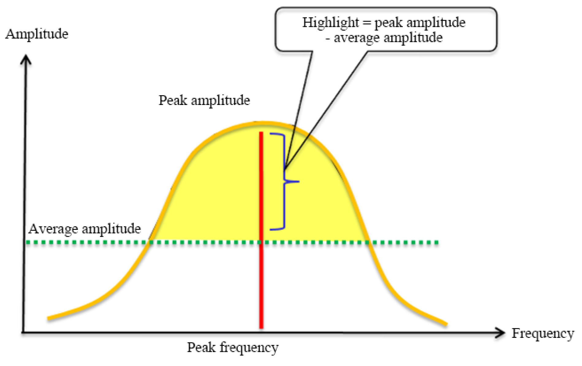
Figure 2.
Frequency anomalies of channels.
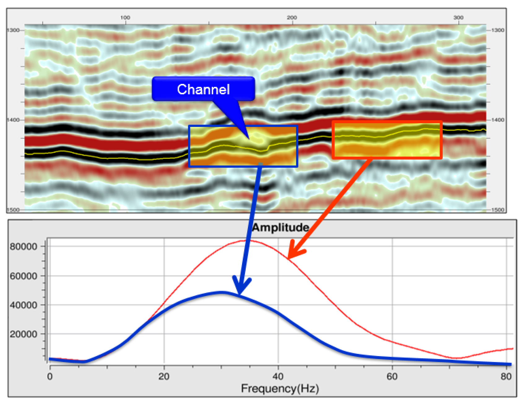
Figure 3.
An example of spectral decomposition.
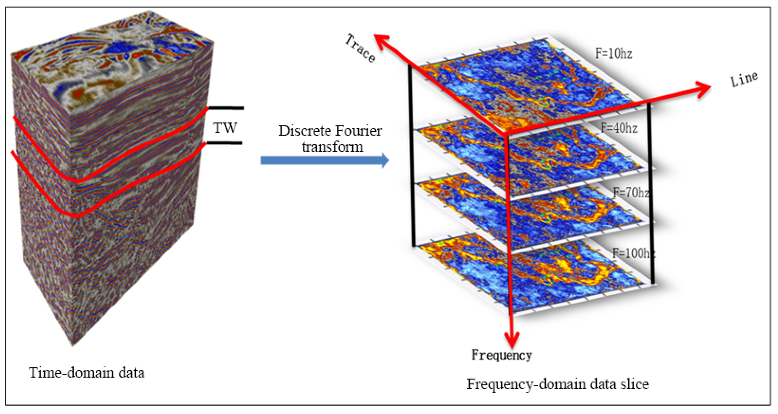
Figure 4.
Amplitude map of layer M-0-1-A and M-0-1-B.
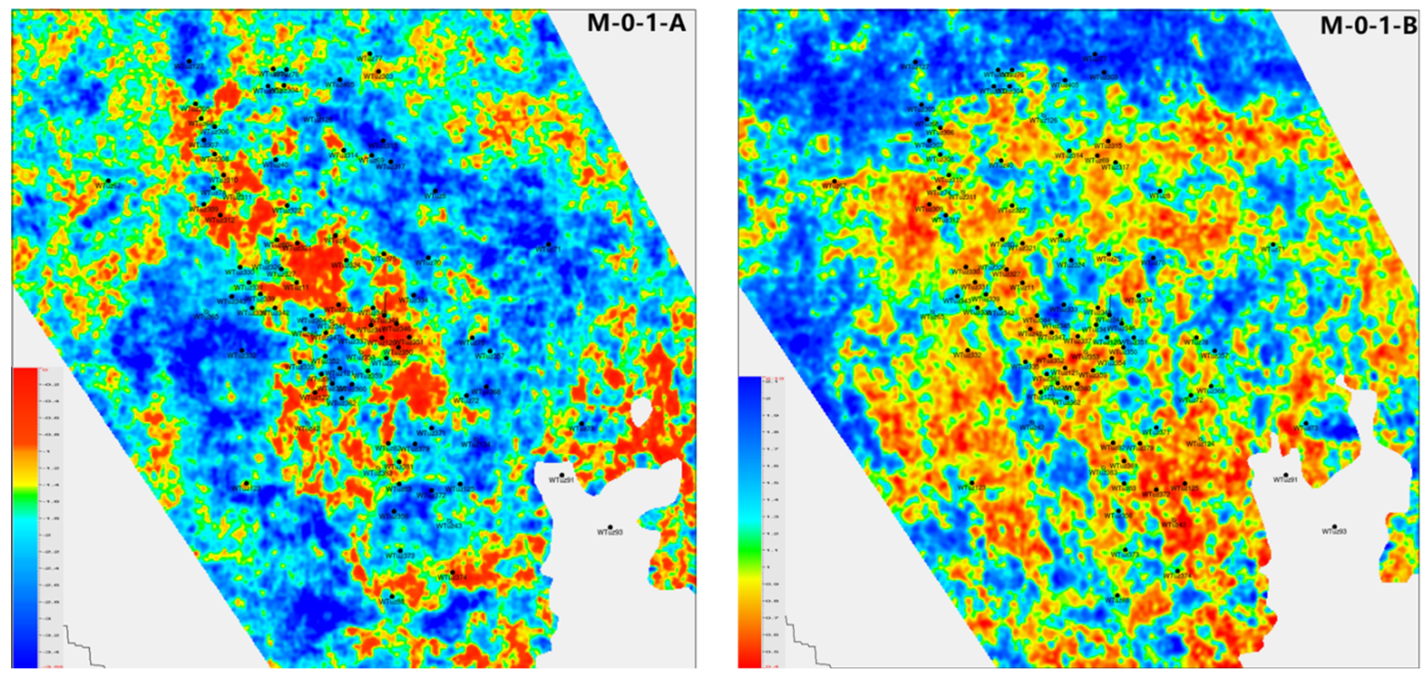
Figure 5.
Amplitude map of layer M-0-2-A and M-0-2-B.
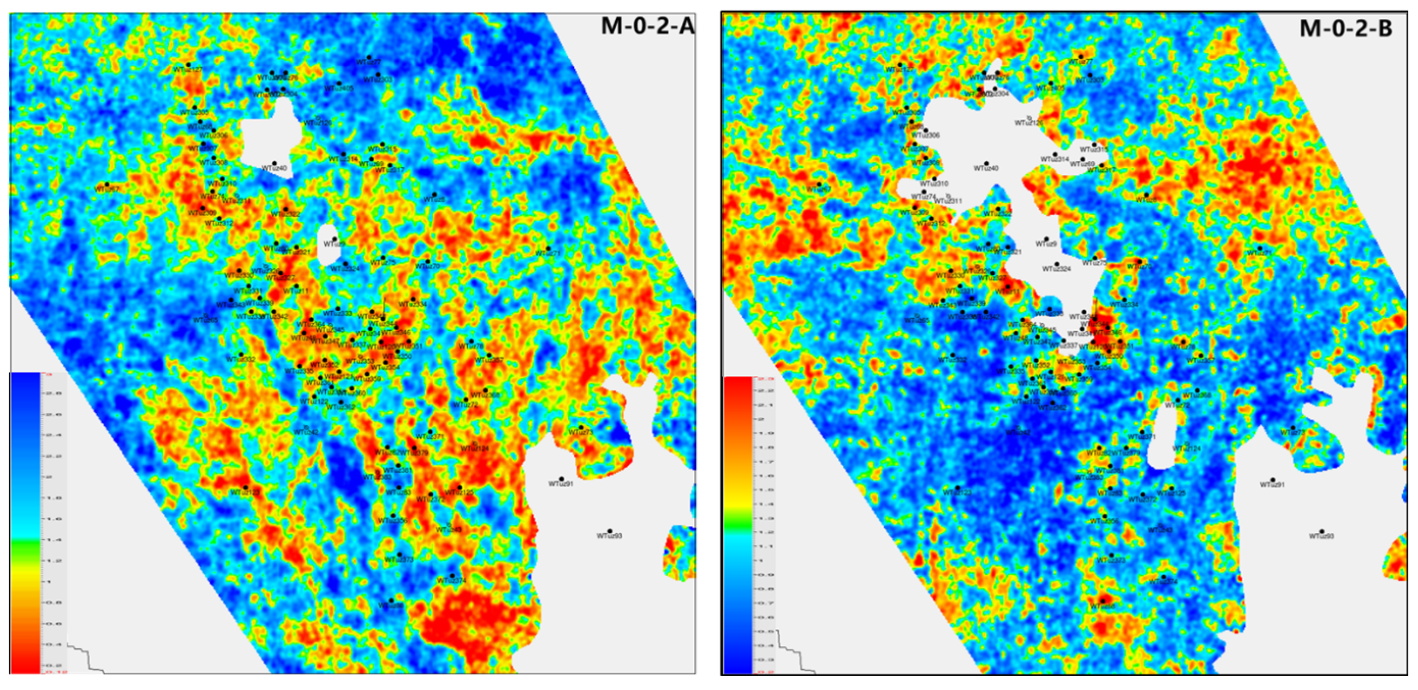
Figure 6.
Spectral decomposition attribute map of layer M-0-1-A and M-0-1-B.
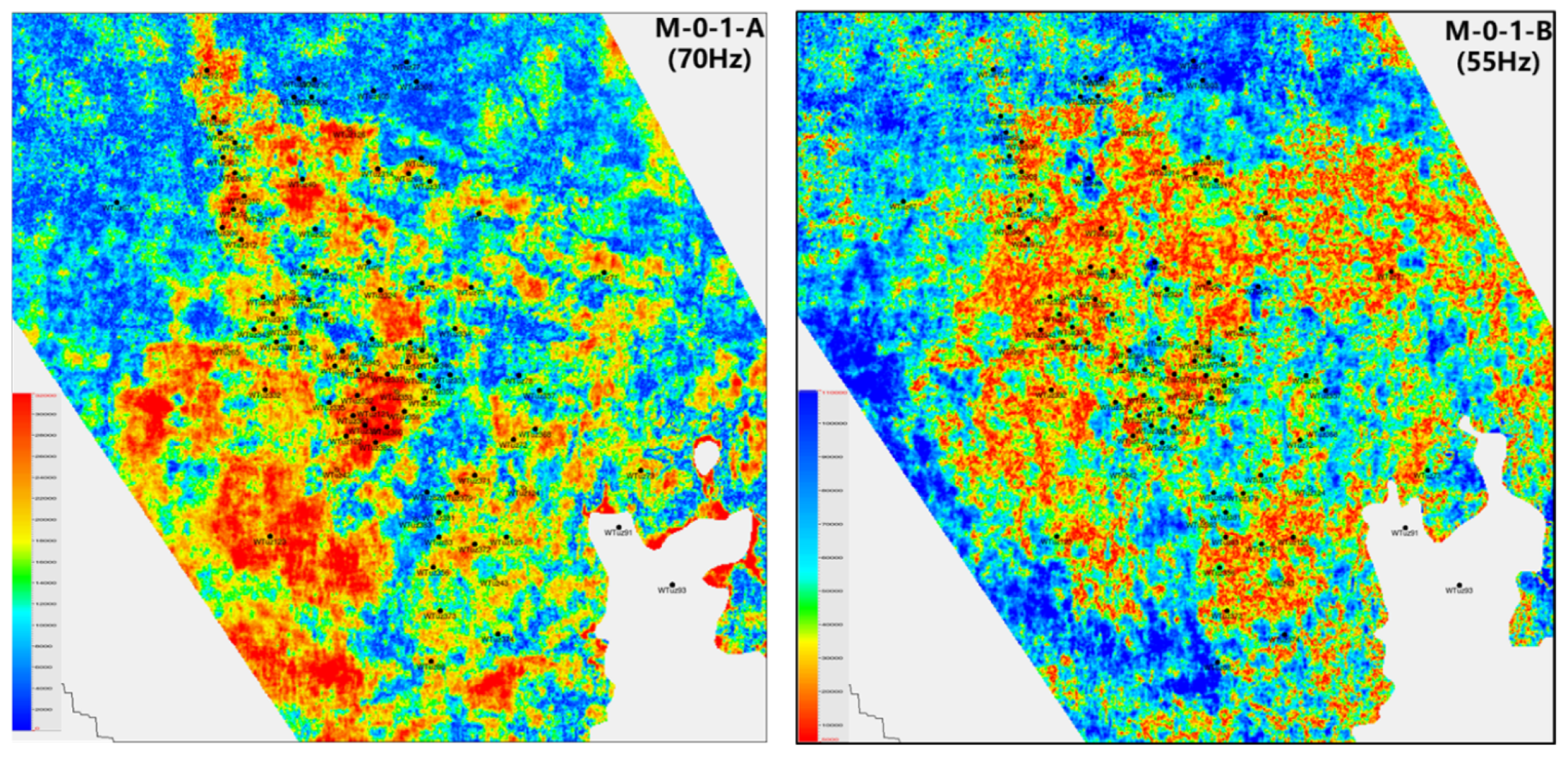
Figure 7.
Spectral decomposition attribute map of layer M-0-2-A and M-0-2-B.
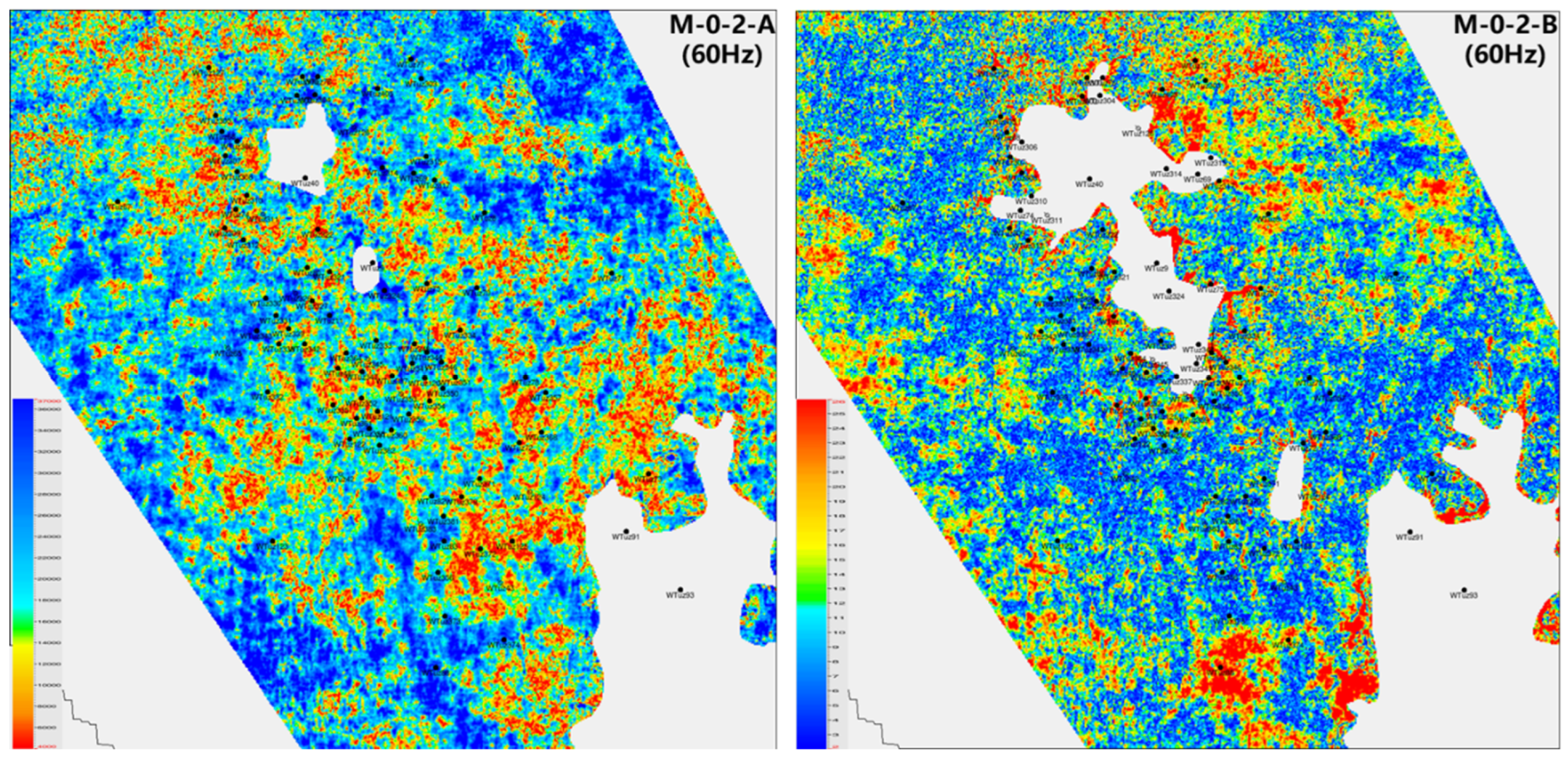
Figure 8.
Histogram of Standardized Sonic Log Distribution.
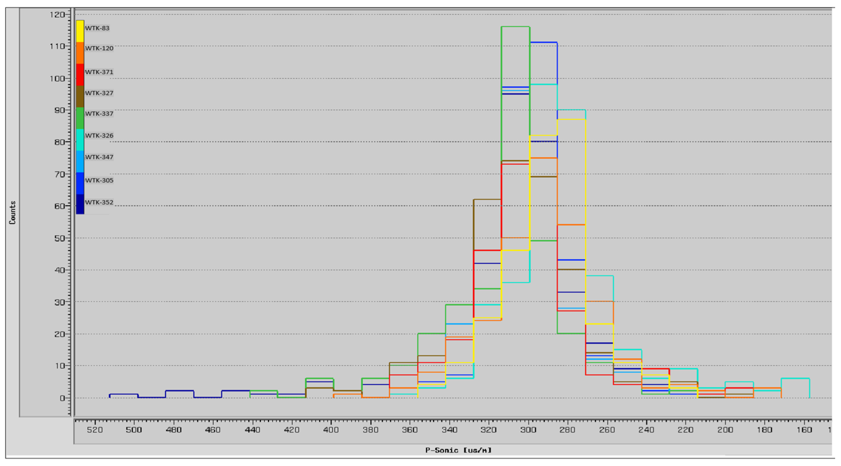
Figure 9.
Seismic Synthetic Seismogram Horizon Calibration of Well 345.
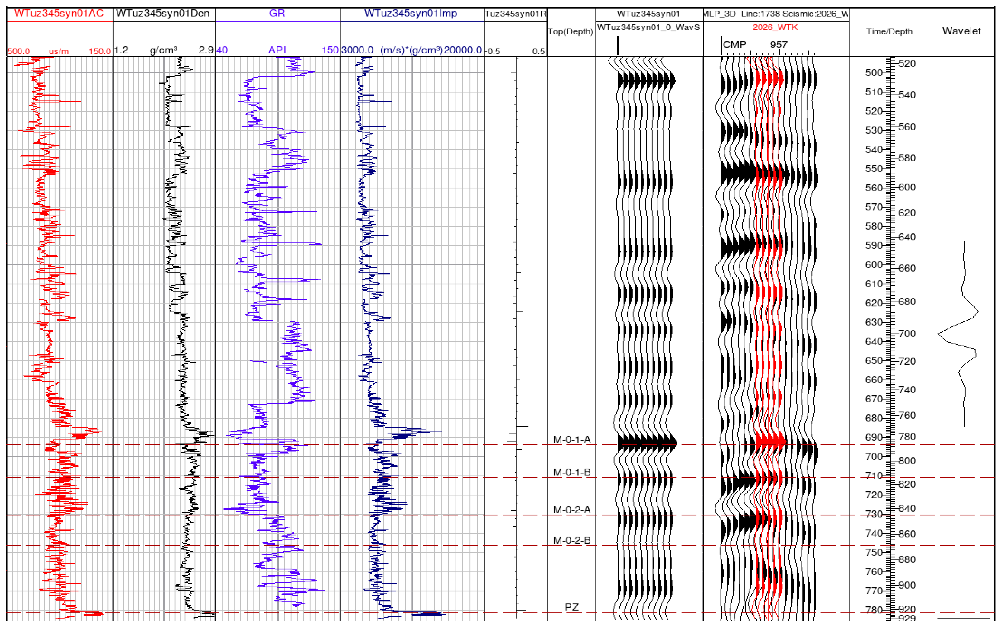
Figure 10.
Seismic Synthetic Seismogram Horizon Calibration of Well 306.
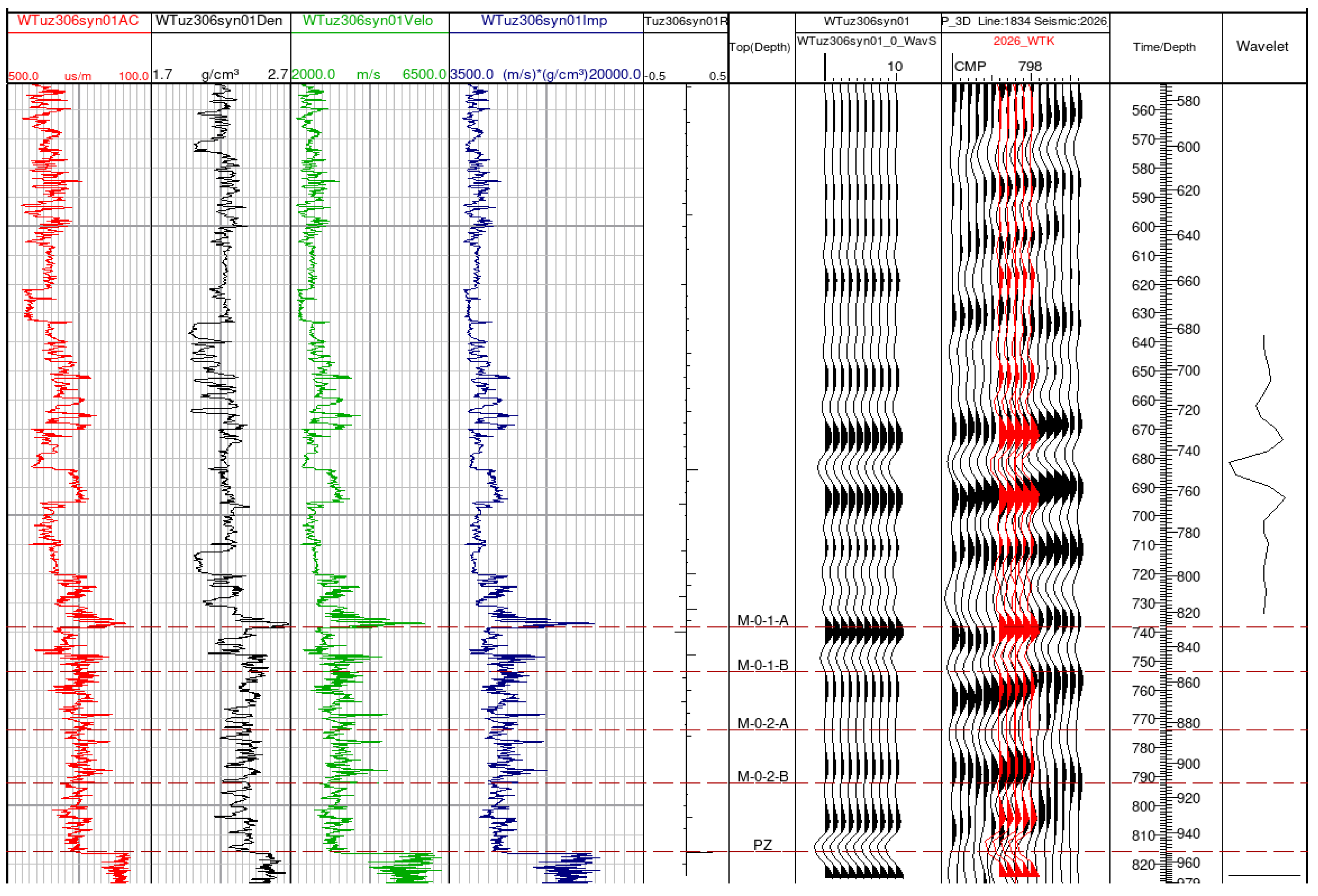
Figure 11.
Schematic Diagram of Average Wavelet Extraction.
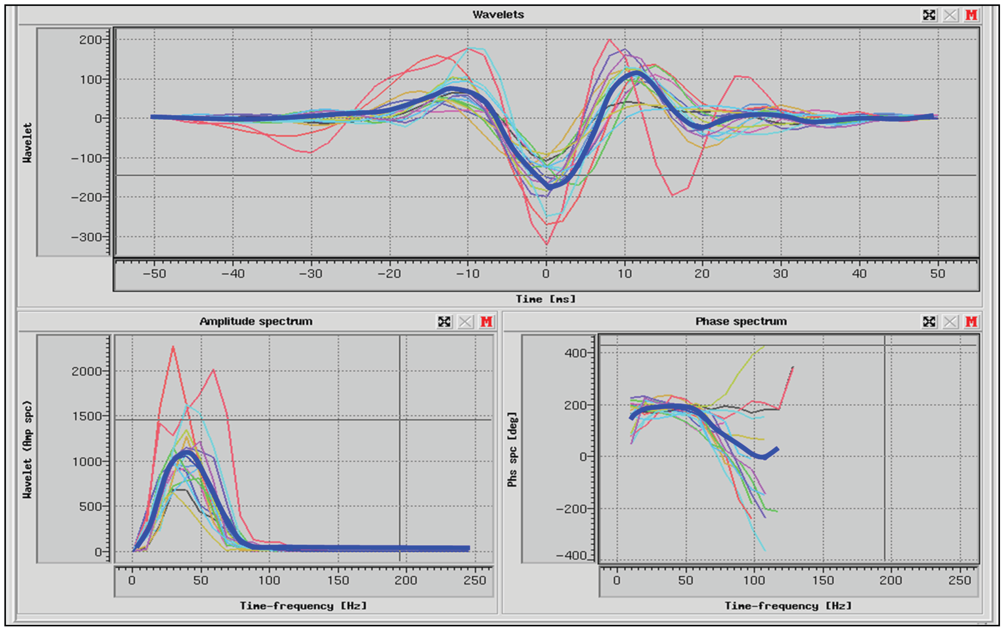
Figure 12.
Initial Low-Frequency Model Profile across Wells 374-43-125-124.
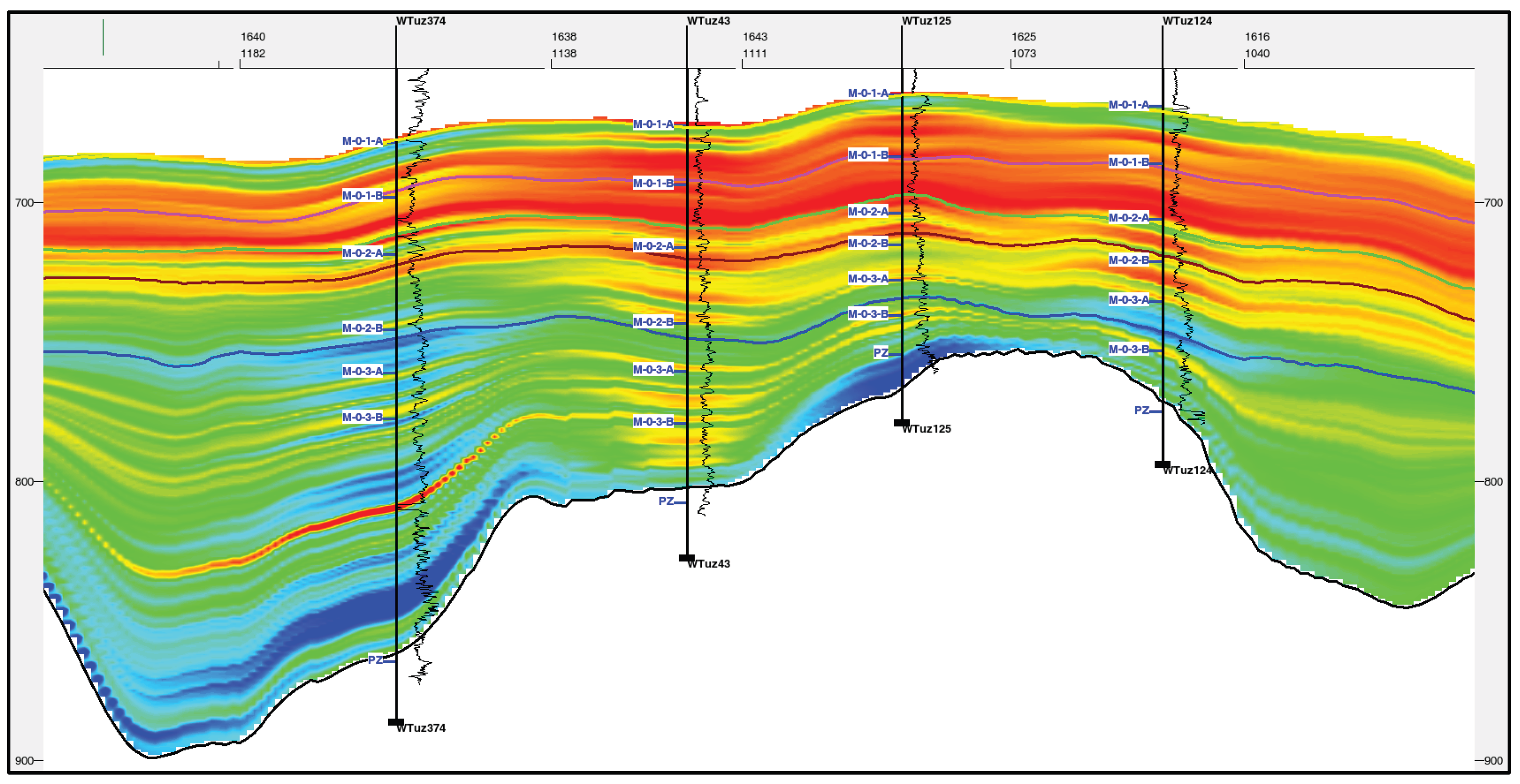
Figure 13.
Acoustic Impedance Inversion Section across Wells 368-82-356.
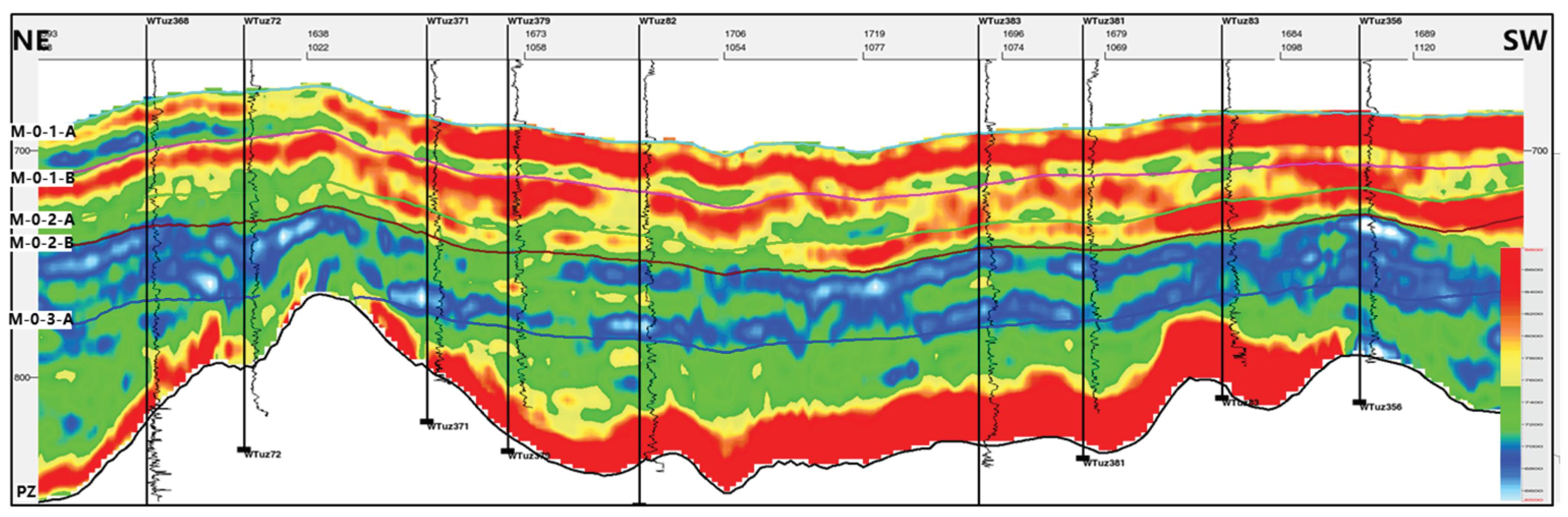
Figure 14.
Acoustic Impedance Inversion Section across Wells 122-353-346.
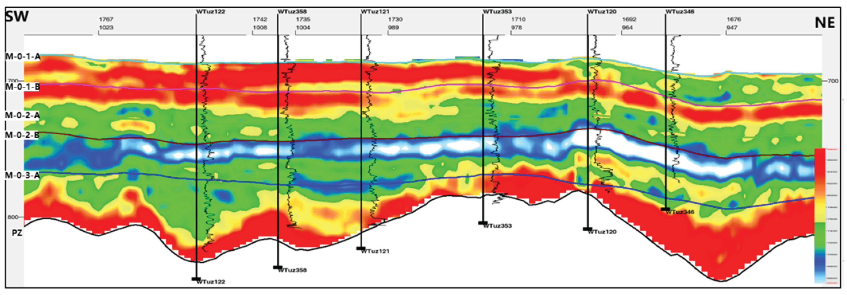
Figure 15.
Acoustic Impedance Inversion Section across Wells 309-308-305.
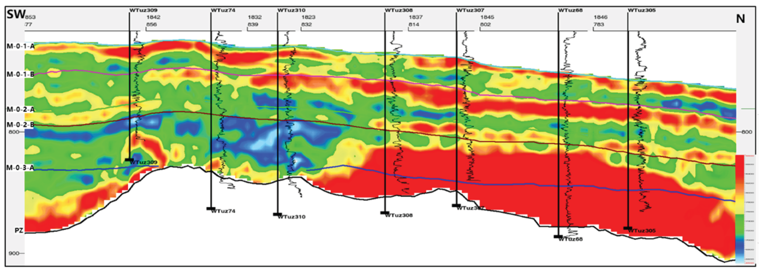
Figure 16.
GR Inversion Section across Wells 368-82-356.
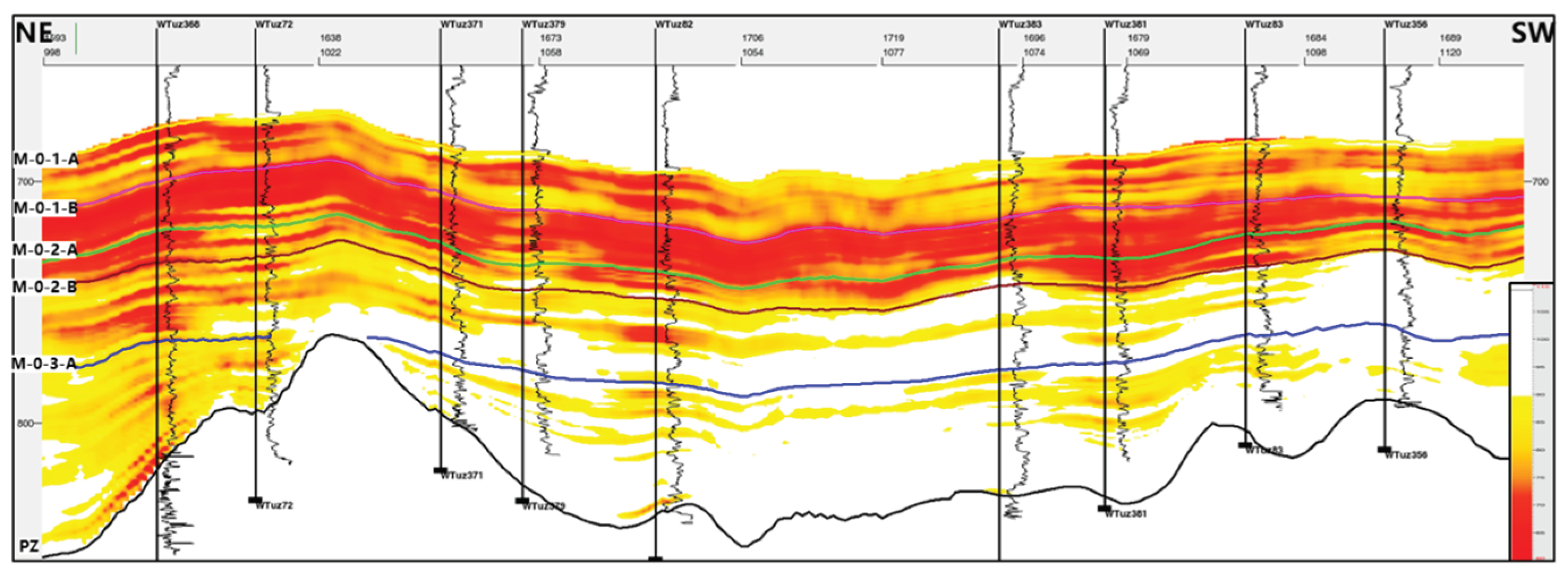
Figure 17.
GR Inversion Section across Wells 122-353-346.
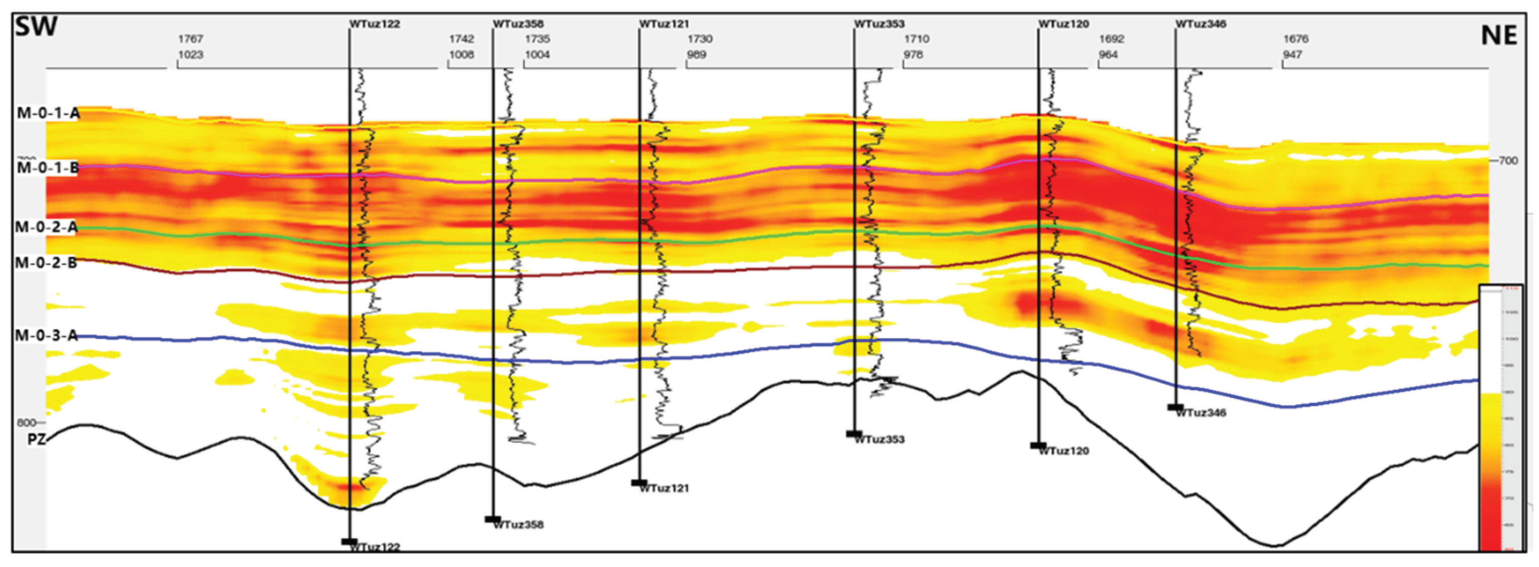
Figure 18.
GR Inversion Section across Wells 309-308-305.
Disclaimer/Publisher’s Note: The statements, opinions and data contained in all publications are solely those of the individual author(s) and contributor(s) and not of MDPI and/or the editor(s). MDPI and/or the editor(s) disclaim responsibility for any injury to people or property resulting from any ideas, methods, instructions or products referred to in the content. |
© 2026 by the authors. Licensee MDPI, Basel, Switzerland. This article is an open access article distributed under the terms and conditions of the Creative Commons Attribution (CC BY) license (http://creativecommons.org/licenses/by/4.0/).
Copyright: This open access article is published under a Creative Commons CC BY 4.0 license, which permit the free download, distribution, and reuse, provided that the author and preprint are cited in any reuse.