

Submitted:
30 September 2026
Posted:
01 October 2026
You are already at the latest version
Abstract
Vehicle dispatching is essential for maintaining supply–demand balance in ride-hailing systems, but existing frameworks separate demand prediction from vehicle allocation, causing a mismatch between prediction accuracy and operational performance. This study proposes a decision-focused end-to-end learning framework that integrates spatiotemporal demand representation and vehicle-to-region dispatching within a unified trainable architecture. The model combines a multi-graph spatiotemporal prediction module with a recurrent Transformer-based dispatching module that iteratively refines vehicle assignments under capacity-aware constraints. A structured loss jointly considers demand prediction, dispatch objectives, and constraint violations, reducing dependence on expensive optimization labels. Experiments on real ride-hailing datasets from Chengdu, Xi’an, and Haikou show competitive dispatching quality and zero capacity-constraint violation rate (CCVR) in the reported city-level comparison. Relative to the Kuhn–Munkres benchmark, the proposed model reduces average online computation time from 242.47 s to 2.47 s, a 98.98% reduction (approximately 98.2-fold acceleration). The decision-oriented mechanism yields operationally useful demand representations, suggesting neural dispatchers offer a scalable approximation for high-frequency operations where responsiveness and feasibility are critical.
Keywords:
decision-focused learning
; ride-hailing
; recurrent Transformer
; vehicle dispatching
; constraint-aware learning
1. Introduction
Ride-hailing platforms have become a core component of urban mobility by matching distributed travel demand with available vehicles [1,2,3]. Their dispatch systems must balance service coverage, vehicle utilization, passenger waiting time, and platform revenue, and these decisions become computationally demanding when updated at high frequency across many vehicles and regions [4,5].
Most practical systems follow a predict-then-dispatch workflow: future demand is first estimated from historical observations, and vehicles are then allocated by an optimization or heuristic procedure [6,7,8]. This modular design is interpretable, but its components are trained under different objectives—demand models minimize statistical error, whereas dispatching models optimize operational quantities such as coverage, revenue, or idle travel [9,10,11]. The prediction with the smallest standalone error is therefore not necessarily the representation that yields the most useful downstream allocation.
Decision-focused learning reduces this mismatch by allowing downstream decision losses to shape the predictive representation [12,13,14]. Reinforcement learning couples state estimation with sequential decisions but requires extensive interaction data and carefully designed rewards [15], while exact and heuristic optimization is too slow to re-solve at high frequency. The central challenge is thus to balance dispatch quality, constraint satisfaction, and online computation time rather than to dominate every baseline.
This study develops an End-to-End Dispatching Model (E2EDM), a decision-focused neural approximation that couples a multi-graph spatiotemporal demand module with a recurrent Transformer to iteratively refine vehicle-to-region assignments. Trained end-to-end with prediction, dispatch-objective, and capacity-constraint terms, it aligns its representations with downstream allocation. It targets dispatch-level decision support and does not model autonomous-vehicle constraints such as battery state of charge or charging availability.
The main contributions of this study are summarized as follows:
- (1)
- We formulate a decision-oriented dispatching problem that unifies idle distance, platform revenue, passenger waiting time, and regional capacity feasibility in a single training objective.
- (2)
- We develop an end-to-end prediction–dispatch framework that links spatiotemporal demand representation to downstream allocation, so predictions are optimized for dispatching utility rather than forecasting error alone.
- (3)
- We design a multi-graph spatiotemporal prediction module that encodes spatial separation, functional similarity, and demand-pattern similarity among regions.
- (4)
- We propose an encoder-only recurrent Transformer that non-autoregressively refines region-level assignment through full-attention global reasoning.
- (5)
- We evaluate the framework on ride-hailing data from three cities, showing competitive dispatching quality, stable capacity feasibility, and substantially lower online computation time than the KM benchmark.
2. Related Work
This section reviews solution algorithms for vehicle dispatching systems, emphasizing computational efficiency and deployment [16,17,18]. Existing methods fall into four categories—traditional optimization, heuristic, machine learning, and reinforcement learning—whose limitations motivate our decision-focused approach.
First, traditional optimization methods provide interpretable, reference-quality solutions when the problem structure is well defined, including mixed-integer programming for intertemporal resource allocation [19], routing and assignment [20], and adaptive KM matching [21]. However, repeatedly solving these models online becomes computationally burdensome as decision variables and dispatch windows grow.
Second, heuristic algorithms offer flexibility and rapid response at the cost of exact optimality. Representative work includes online insertion heuristics that anticipate future demand [22], hybrid assignment–optimization for dial-a-ride problems [23], non-myopic relocation incorporating long-term objectives [24], batch order dispatching with short-term demand [25], variable neighborhood search for demand-responsive transit and shared autonomous vehicles [26,27], hybrid multi-criteria frameworks for rural last-mile planning [28], and green or time-dependent routing solved by swarm-based metaheuristics [29,30,31,32]. Despite this flexibility, heuristics rely on hand-designed rules and domain knowledge [33,34], limiting their adaptability and generalization in dynamic, heterogeneous urban environments [35,36]; these limitations motivate more data-driven alternatives [37,38].
Third, data-driven machine learning methods learn dispatching policies directly from large-scale historical data, improving adaptability over rule-based heuristics [39,40,41]. Guo et al. [42,43] integrate data-driven demand estimation into optimization-based dispatching, classifying approaches into order matching, vehicle repositioning, and joint modeling. Such methods improve efficiency and accuracy but face scalability and generalization challenges in large-scale deployment.
Fourth, reinforcement learning (RL) addresses sequential decision making through environment interaction [44]. Prior work formulates taxi dispatching as a Markov decision process with multi-agent assignment and repositioning [45,46,47], and hybrid methods combine deep RL with integer programming for assignment and rebalancing [48], while others incorporate passenger behavior and driver heterogeneity [49,50]. Shared-bicycle studies explore RL-based rebalancing and predictive scheduling [51,52], and large-scale implementations adopt multi-agent actor–critic frameworks [53]. These methods are expressive but their interaction requirements, training cost, and reward design complicate deployment.
Despite this progress, several challenges remain (Table 1). Specifically, most approaches exhibit the following limitations:
- (1)
- Prediction and dispatching objectives are often optimized separately, though lower prediction error does not guarantee better allocation.
- (2)
- Optimization and heuristic methods provide strong reference solutions, but their online cost grows with instance size and dispatch frequency.
- (3)
- Learning-based dispatchers must balance operational objectives, capacity constraints, and scalable inference.
These gaps motivate a decision-focused neural approximation rather than a claim that learning should replace optimization. The proposed framework couples prediction and dispatching during training, incorporates capacity terms, and moves most computation offline, providing fast, constraint-aware assignments while retaining optimization and heuristic methods as high-quality references [19,54].
3. Problem Formulation
This section begins by introducing the fundamental definitions and problem formulation that underpin our approach. This is followed by a comprehensive description of the proposed vehicle dispatching model, which jointly considers multiple optimization objectives from both the platform and user perspectives, ensuring a balanced and holistic dispatching strategy.
DEF 1. SERVICE BLOCK. Let S denote the given geographic region, with longitude boundaries and , and latitude boundaries and . The region is partitioned into service blocks , as defined in Equations (1)–(3). In this partition, the length and width of each service block are given by:
DEF 2. TIME WINDOWS. The 24-hour day is evenly divided into intervals of equal duration, represented by the set .
DEF 3. SERVICEABLE VEHICLE. All available service vehicles are represented by the set where denotes the total number of available vehicles.
DEF 4. PASSENGER DEMAND. Passenger demand is denoted by , defined as the total number of user orders submitted within service block during time window .
DEF 5. DECISION VARIABLE. Let the time-indexed decision variable indicate whether vehicle is assigned to service block during time window :
We consider three operational quantities: vehicle idle distance, platform income, and passenger waiting time. Their weighted combination is used as a differentiable decision-oriented training signal; it is not presented as an exact mathematical program solved online at every window:
Here, , , and denote the corresponding quantities for vehicle n at time . The coefficients , , and control their relative importance.
Specifically,
where denotes the distance traveled by vehicle n to service block , and represents the average revenue from historical orders.
The standard one-to-one assignment problem can be solved in polynomial time by Hungarian-type algorithms. However, when regional capacity constraints, multiple operational objectives, rolling time windows, and large online instances are considered together, repeatedly solving optimization or heuristic models can become computationally burdensome. This motivates learning a fast approximation that is evaluated against optimization-based references.
4. Methodology
We propose an End-to-End Prediction-Dispatch Model (E2EDM) composed of two modules: prediction module and dispatching module. Section 4.1 outlines the overall architecture, Section 4.2 details the prediction module, Section 4.3 presents the dispatching module, and Section 4.4 introduces the training objective and optimization procedure.
4.1. Overview of The End-to-End Dispatching Model
The proposed model encompasses the full dispatching workflow, spanning from historical order data ingestion, through pattern learning, to final vehicle dispatching decisions and assignment outputs. The overall architecture is structured into two main stages, as illustrated in Figure 1.
4.1.1. Offline Learning
During the offline learning phase, the prediction and dispatching modules are jointly optimized based on a grid-based spatial partitioning of the urban area and historical order data. Specifically, we construct multiple heterogeneous graph structures that capture service block adjacency and historical mobility patterns. A Multi-Graph Convolutional Network (MGCN) is employed to extract spatial dependency features across service blocks. These spatial embeddings are then fed into an LSTM-based encoder-decoder architecture to model the temporal dynamics of demand evolution, enabling accurate prediction of order distributions across future time windows.
The prediction outputs are embedded as structured inputs into the dispatching module, enabling the latter to generate vehicle-to-block assignment strategies that optimize platform-level objectives such as idle distance minimization, revenue maximization, and supply-demand balance. Unlike traditional pipeline designs, where prediction and dispatching are trained independently, our model implements a fully differentiable architecture wherein both modules are jointly optimized in an end-to-end manner.
Specifically, gradients from the dispatching loss can propagate through the Transformer layers into the upstream prediction module. The architecture is therefore end-to-end trainable and structurally coupled, allowing demand representations to be shaped by both prediction error and downstream dispatch objectives. The experiments evaluate the integrated framework, but do not claim that this coupling universally dominates independently trained prediction models.
Service-block capacity limits are incorporated through differentiable penalty terms. These terms encourage feasible assignments rather than mathematically guaranteeing feasibility for every possible input.
4.1.2. Online Planning
In the online planning phase, the trained model predicts upcoming demand and generates vehicle-to-block assignments without repeatedly solving the KM reference problem. Most computation is shifted to offline training, while online inference remains at the seconds level on the reported hardware.
4.2. Prediction Module
To capture prior knowledge of passenger demand pattern, we propose a Spatiotemporal Multi-Graph Convolution (STMGC) module that effectively models the complex spatial and temporal dependencies among service blocks. The structure of the module is illustrated in Figure 2. The module jointly captures spatial correlations between different regions and temporal dynamics in historical demand patterns, enabling more accurate demand prediction. We propose a Spatiotemporal Multi-Graph Convolution (STMGC) module that jointly models spatial and temporal dependencies among service blocks (Figure 2), providing reliable demand representations for downstream dispatching.
Since a single graph cannot capture the multidimensional correlations among service blocks, we construct three graphs from distinct perspectives: geographical proximity, functional similarity, and demand heat similarity. Each graph encodes spatial relationships from a distinct perspective: geographical proximity, functional similarity, and historical demand heat similarity. This multi-view graph construction enables a more comprehensive and nuanced representation of the associative features among service blocks, thereby enhancing the model’s capacity to capture realistic spatial interactions.
GRAPH 1. DISTANCE-COST GRAPH. The distance-cost graph records the spatial separation between service blocks. Each node corresponds to a grid cell, and a larger edge value indicates greater separation rather than stronger similarity. The subsequent normalization and learned transformations determine how this cost information contributes to the representation. Specifically, for any two blocks and , their Euclidean distance is defined as follows:
Here, and denote the centroid coordinates of block i. This graph provides explicit geographic cost information that complements the functional and historical-demand similarity graphs.
GRAPH 2. POI SIMILARITY GRAPH. Service blocks with similar functional attributes—such as commercial centers, residential neighborhoods, or entertainment districts, often exhibit analogous patterns of demand fluctuation. To quantify these functional similarities, we construct a Point-of-Interest (POI) similarity graph, in which edge weights reflect the degree of overlap in POI category distributions between blocks. This graph provides valuable contextual information that complements purely spatial and temporal signals, enhancing the model’s ability to generalize across diverse urban environments. Specifically, for each block , we generate a functional feature vector by aggregating the distribution of different categories of POIs within that block. The POI similarity between any two blocks is computed as shown in Equation (10):
Here, represents the POI similarity between service blocks i and j, denotes the POI feature vector of service block i, where is the count of POIs of category k within block i.
GRAPH 3. HEAT GRAPH. The Heat Graph captures dependencies between service blocks that, although geographically distant and functionally dissimilar, exhibit highly similar patterns of demand evolution over time. For instance, a commercial district and a medical center—despite their spatial separation and distinct land-use functions—may display comparable temporal trends in order demand. To model these latent demand correlations, we construct a demand heat similarity graph, in which each node represents a service block and the edge weights are determined by the pairwise correlation between their historical passenger demand time series. This approach enables the model to identify and leverage functional analogies that are not evident from geographic or categorical features alone. By connecting service blocks with similar demand dynamics, the Heat Graph enhances the model’s capacity to generalize and adapt to complex, real-world dispatching scenarios. Specifically, the heat graph is defined as shown in Equation (11):
Here, and denote the historical demand sequences of blocks i and j, respectively. Equation (11) is the Pearson correlation coefficient, with a small added for numerical stability.
After constructing the three heterogeneous graphs: representing geographical proximity, functional similarity, and demand heat similarity—we perform graph convolution operations on each graph in parallel. This allows us to extract service block embeddings from multiple distinct perspectives simultaneously. The resulting multi-view embeddings are then aggregated through a feature fusion mechanism to generate a unified representation for each service block. This fused representation serves as the input to the downstream demand prediction module. By jointly modeling the heterogeneous graph structures, the proposed approach effectively enhances the model’s ability to capture complex inter-block dependencies across spatial, functional, and temporal dimensions. This leads to more informative and robust feature representations, ultimately contributing to improved accuracy in predicting future demand patterns.
Here, denotes the activation function, A represents the adjacency matrix corresponding to the input graph, is the output of the previous layer, and denotes the weight matrix.
To extend the capability of the GCN for handling multi-view graph structures, we adopt an enhanced multi-graph convolution approach [55], which can be formulated as follows:
where denotes the symmetrically normalized adjacency matrix, and represents the adjacency matrix of each graph type.
To further integrate different types of service block relationship graphs, we employ a Multi-Graph Convolution (MGC) mechanism [56]. Specifically, for the constructed heterogeneous graphs, the MGC operation is defined as follows:
To improve computational efficiency, we adopt a Chebyshev polynomial approximation to replace the standard graph convolution operation, thereby accelerating the convolution process for each graph. This approximation is formulated as:
where represents the K-order Chebyshev polynomial function of the graph Laplacian, and denotes the feature transformation matrix. This mechanism significantly reduces computational complexity while preserving accurate feature propagation across heterogeneous graph structures, thereby enhancing the model’s efficiency in encoding spatial dependencies.
To capture the temporal evolution patterns of block-level demand, we further incorporate an LSTM Encoder-Decoder architecture, which effectively models sequential dependencies over time. The architecture follows a sequence-to-sequence (Seq2Seq) framework, consisting of an encoder that captures historical temporal patterns and a decoder that generates future demand forecasts.
Specifically, the model first applies multi-graph convolution to historical order data across multiple time windows. Within each time window, graph convolutions are performed in parallel across the distance graph, POI similarity graph, and heat graph, extracting spatial features from distinct perspectives. These multi-view features are then aggregated through a weighted fusion operation, yielding a comprehensive spatial representation for each time window, denoted as . For a sequence of k time windows, this yields a spatial feature sequence:
This sequence serves as the encoder input to capture long-term temporal dependencies in block features and is compressed into a fixed-length internal representation, which is passed as the hidden state to the decoder. The decoder then takes the encoder’s final state as its initial state and sequentially predicts the output demand estimates:
The pseudocode below outlines the procedure of the STMGC prediction module.
| Pseudocode 1: STMGC prediction module | |
| 1: | Input: historical demand sequence , multi-graph adjacency matrices |
| 2: | Initialize parameters of GCN layers and LSTM encoder |
| 3: | for to T do |
| 4: | for each graph do |
| 5: | Compute normalized adjacency matrix: |
| 6: | Perform Chebyshev GCN convolution: |
| 7: | end for |
| 8: | Fuse features from all graphs: |
| 9: | end for |
| 10: | Get spatial-temporal sequence: |
| 11: | Feed sequence into LSTM encoder to capture temporal patterns |
| 12: | Use decoder to predict future demand: |
| 13: | Output: predicted demand sequence |
4.3. Dispatching Module
The dispatching module uses an encoder-only recurrent Transformer to represent coupled vehicle-to-region decisions. Unlike autoregressive sequence generation, all vehicle representations are updated in parallel with non-causal full attention. A recurrent inference mechanism feeds the hidden representation from one reasoning round into the next, enabling non-autoregressive iterative refinement of the assignment distribution.
The module has three features: (1) encoder-only parallel updates, where all vehicle states are updated simultaneously rather than autoregressively [57]; (2) recurrent refinement, where multiple self-attention rounds reuse the previous hidden state [58] (evaluated in Table 6); and (3) non-causal full attention over the global vehicle and block state, supporting coordinated reasoning (Figure 3).
In the modeling process, the dispatching module receives two key input matrices: the demand distribution matrix , which records the demand information for each service block within a specified time window. This matrix is used to enforce column constraints, ensuring that the number of vehicles assigned to each block does not exceed its corresponding demand capacity. Additionally, the vehicle distribution matrix captures the current vehicle distribution status.
We first embed the vehicle distribution into token and positional representations and , where the former projects vehicle features into a shared latent space and the latter preserves each vehicle’s identity and relative position. Meanwhile, is a randomly initialized positional encoding vector of dimension , used to preserve the identity and relative position of each vehicle within the fleet, ensuring that the model can distinguish between different vehicles.
The proposed Recurrent-Transformer model adopts a stacked architecture integrated with a recursive looping mechanism, consisting of M self-attention blocks and N recursive iterations. Through this multi-step reasoning framework, the model iteratively refines dispatching decisions, progressively improving the alignment between vehicle assignments and dynamic demand patterns:
Here, denotes the initial hidden state of the n-th recursive iteration. In particular, the initial hidden embedding input is defined as . represents the m-th Transformer block, which performs self-attention mechanisms and feedforward network operations at each layer. The operator denotes layer normalization, which stabilizes the training process. denotes the output layer weights, and denotes the neural network outputs.
To enhance the model’s ability to capture diverse subspace features within the global system state, we incorporate the multi-head attention mechanism, which enables the model to jointly attend to information from different representation subspaces.
Assume that the hidden state is linearly projected into h attention heads, each with a reduced feature dimension of:
For the k-th attention head, in the n-th recursive iteration and the m-th Transformer block, the , , and representations are defined as follows:
The scaled dot-product attention weights are defined as follows:
The attention output and its projected head representation are then computed as:
By concatenating the outputs of all attention heads and applying a linear transformation, we derive the aggregated representation:
Finally, the overall update operation of each Transformer block is expressed as follows:
Here, the subscript k indicates the query , key , and value matrices corresponding to the k-th attention head. denotes the attention-weight matrix, and is the corresponding value-weighted attention output. denotes the dimensionality of the key vectors and scales the dot product to improve numerical stability. projects each head output, while projects the concatenated multi-head representation into the desired output dimension.
This multi-head attention design allows the model to simultaneously model vehicle–vehicle interactions, block-block correlations, and cross-entity dependencies, significantly enhancing its capacity to perform global collaborative reasoning in complex dispatching scenarios. The pseudocode below outlines the procedure of the Recurrent-Transformer dispatching module.
| Pseudocode 2: Recurrent-Transformer Dispatching Module | |
| 1: | Input: Vehicle feature set V with features (location, idle time, capacity), region set with predicted demand , recursion step N, transformer block number M. |
| 2: | Token embedding matrices and . |
| 3: | Set . |
| 4: | For to N do |
| 5: | If , set . |
| 6: | For to M do |
| 7: | For each head to h do |
| 8: | . |
| 9: | . |
| 10: | . |
| 11: | . |
| 12: | ; . |
| 13: | end for |
| 14: | . |
| 15: | . |
| 16: | end for |
| 17: | end for |
| 18: | Output: Final dispatch decision matrix . |
4.4. Loss Function
To jointly optimize demand prediction, dispatch objectives, and constraint penalties, we design a structured loss that supports two training strategies: KM-guided optimization (KMGO) and constraint-guided optimization (CGO). KMGO uses KM-generated reference assignments as supervised guidance, whereas CGO relies on the differentiable dispatch objective and structural constraint penalties without requiring KM labels.
The first component of the loss function is the Prediction Loss , which quantifies the model’s performance in predicting future demand trends. This is implemented using the Mean Squared Error (MSE) between the predicted and actual demand distributions across service blocks:
where and denote the predicted and ground-truth demand values, and k is the total number of service blocks.
To optimize the vehicle dispatching module, we define two complementary types of dispatching loss that accommodate different training scenarios and data availability:
(1) KM-guided optimization loss. When KM reference assignments are available, the model minimizes the discrepancy between the objective values of its predicted assignment and the reference assignment.
(2) Constraint-guided optimization loss. In CGO, reference assignments are not used. The model is guided by the differentiable dispatch objective and structural constraint penalties. This reduces dependence on optimization labels, although it does not constitute a proof of optimality.
Let represent the reference assignment indicating the target service block for each vehicle. Given the model’s predicted dispatching plan P, we evaluate the quality of the dispatching solution based on key operational metrics such as empty mileage C, platform revenue I, and passenger waiting time T.
Accordingly, in the supervised setting, the single-step dispatch loss is defined as the difference between the expected objective value derived from the model’s output and the corresponding value from the reference assignment:
In the absence of reference assignments, we define the single-step unsupervised dispatch loss as:
To account for the recursive nature of the Recurrent-Transformer architecture, we accumulate the single-step losses across all recursive iterations and Transformer blocks to compute the overall dispatch loss:
When applying unsupervised loss, to ensure that the dispatching solutions adhere to real-world operational constraints, we incorporate a Constraint Embedding Mechanism, which introduces explicit structural loss terms to encode key scheduling rules:
(1) Row Constraint (Vehicle Single Assignment): Each dispatched vehicle is assigned to one service block.
(2) Column Constraint (Block Capacity Limitation): The number of vehicles assigned to block j must not exceed its demand capacity .
The overall constraint loss is then defined as a weighted combination:
where and are hyperparameters balancing the influence of each constraint.
The total loss is a weighted combination of all components:
where or is applied depending on the training strategy, and and are coefficients controlling the relative importance of each component.
The constraint penalties encourage single assignments and capacity-aware allocations. Their empirical contribution is assessed by the loss ablation in Table 7; no hard feasibility guarantee is assumed.
5. Experiments
This section evaluates prediction accuracy, dispatch quality, constraint behavior, and online computation time on three real-world ride-hailing datasets.
The experimental data are anonymized ride-hailing order records from Didi Chuxing, collected in three cities—Chengdu, Xi’an, and Haikou—including order timestamps, pickup and drop-off locations, trip durations and distances, and vehicle status. Experiments were implemented in Python 3.10 with PyTorch 1.13 and mixed-precision training on an RTX 3060 Ti GPU. Table 2 presents the hyperparameter configuration.
5.1. Evaluation of Prediction Module
We evaluate the demand prediction module using Mean Absolute Error (MAE) and Root Mean Square Error (RMSE), comparing against statistical, machine learning, and deep learning baselines.
Table 3 and Figure 4 summarize the prediction results. The proposed model achieves competitive accuracy across the three cities and improves substantially over the statistical and several machine-learning baselines. ASTGCN, however, obtains lower MAE and RMSE in all three datasets. This result is expected because ASTGCN is optimized specifically for standalone forecasting, whereas the proposed prediction module is trained within a decision-oriented objective that also reflects downstream dispatching. Accordingly, Table 3 should be interpreted as evidence that the integrated model retains a reasonable forecasting capability, not as evidence of best-in-class prediction accuracy.
Table 4 reports the graph ablation. Removing the distance-cost graph degrades both MAE and RMSE, indicating that geographic separation is important. Removing the POI or heat graph increases MAE but decreases RMSE. The graph views therefore have heterogeneous effects on average error and large-error sensitivity. Multi-graph fusion is interpreted here as a decision-oriented representation design rather than a mechanism that minimizes every standalone forecasting metric.
5.2. Evaluation of Dispatching Module
This subsection evaluates the learned dispatcher on representative instances from Chengdu, Xi’an, and Haikou. KM provides a reference solution for the underlying bipartite matching component. Because the complete evaluation also includes regional capacity and supply–demand metrics, KM is treated as a benchmark rather than a globally optimal solution to every operational objective considered in this study.
Figure 5 illustrates one dispatching instance on a grid. The learned allocation broadly follows the spatial pattern of the KM reference while not reproducing it exactly. The example is qualitative; the aggregate comparisons in Table 5 and Table 8 provide the quantitative evidence.
To further quantify the model’s performance, we define the supply-demand equilibrium ratio (SDER) and the capacity constraint violation rate (CCVR) as assessment metrics. The SDER is formulated as: , where supply–demand equilibrium refers to balancing supply and demand across all service blocks. This metric quantifies the degree of global coordination between vehicle supply and order demand and particularly reflects whether the dispatching solution can maintain basic service coverage in low-demand service block under resource-constrained conditions, thereby indicating the robustness and fairness of the strategy. The CCVR is defined as: , which measures the extent to which the dispatching plan reasonably allocates vehicle resources and avoids excessive vehicle aggregation in certain service blocks.
As shown in Table 5, the proposed model achieves an average SDER of 92.95% across the three cities and maintains zero CCVR in all cases. It improves SDER over KM, IKM, and AVNS, while FSR obtains higher SDER in Chengdu and Xi’an and the proposed model obtains the highest value in Haikou. The results therefore support competitive dispatch quality and stable capacity behavior, rather than strict dominance over every baseline. The zero CCVR is consistent with the use of capacity-aware loss terms.
To further investigate the impact of architectural design choices on model performance, we conducted a comprehensive ablation study by varying key hyperparameters of the Recurrent Transformer architecture. The results of these experiments are summarized in Table 6.

Table 6.
Performance analysis with different M/N combinations.
| Configuration | Instance 1 | Instance 2 | Instance 3 | Instance 4 | ||||
|---|---|---|---|---|---|---|---|---|
| SDER | CCVR | SDER | CCVR | SDER | CCVR | SDER | CCVR | |
| M1N16 | 81.33% | 0% | 81.51% | 3% | 83.13% | 0% | 80.62% | 5% |
| M1N32 | 84.59% | 0% | 83.77% | 0% | 86.41% | 0% | 85.42% | 1% |
| M2N16 | 89.19% | 0% | 90.21% | 1% | 88.79% | 0% | 86.94% | 1% |
| M2N32 | 91.83% | 0% | 92.44% | 0% | 93.13% | 0% | 91.39% | 0% |
| M4N16 | 92.61% | 0% | 93.92% | 0% | 91.85% | 0% | 92.83% | 0% |
| M4N32 | 89.37% | 0% | 89.18% | 1% | 89.71% | 0% | 90.38% | 0% |
| M32N1 | 72.21% | 3% | 73.36% | 4% | 74.31% | 2% | 71.76% | 6% |
Increasing recurrent depth generally improves SDER up to a moderate level, but additional depth does not necessarily yield further gains. In particular, M4N32 performs below M4N16 on the four reported instances. Recurrent refinement is useful, whereas excessive depth may introduce redundant reasoning or optimization difficulty.
Figure 6 shows that SDER increases and stabilizes during training, while CCVR decreases toward zero after an intermediate fluctuation. This indicates convergence toward higher supply–demand balance and lower capacity violations under the reported configuration.
To examine positional encoding, we remove it from the M1N16 configuration. Figure 7 shows a substantial deterioration in the allocation pattern, and the reported CCVR increases by 2236% relative to the encoded configuration. This result indicates that positional information is important for distinguishing service blocks and encouraging stable, capacity-aware assignments in this setting.
Table 7 compares KM-guided optimization (KMGO) and constraint-guided optimization (CGO). CGO retains zero CCVR without KM-generated labels, although its SDER is generally lower than KMGO. Removing the constraint loss from CGO raises CCVR to 11.24–21.33% and also reduces SDER. This ablation supports the role of the constraint penalties in encouraging capacity-aware decisions under limited supervision.
Table 7.
Loss function ablation experimental results.
| Configuration | Instance 1 | Instance 2 | Instance 3 | Instance 4 | ||||
|---|---|---|---|---|---|---|---|---|
| SDER | CCVR | SDER | CCVR | SDER | CCVR | SDER | CCVR | |
| KMGO | 92.61% | 0% | 91.92% | 0% | 90.85% | 0% | 91.13% | 0% |
| CGO | 89.23% | 0% | 87.91% | 0% | 89.14% | 0% | 91.44% | 0% |
| CGO- | 81.33% | 15.72% | 82.86% | 21.33% | 84.15% | 16.51% | 82.49% | 11.24% |
Figure 8.
Performance comparison of loss function ablation experiment.
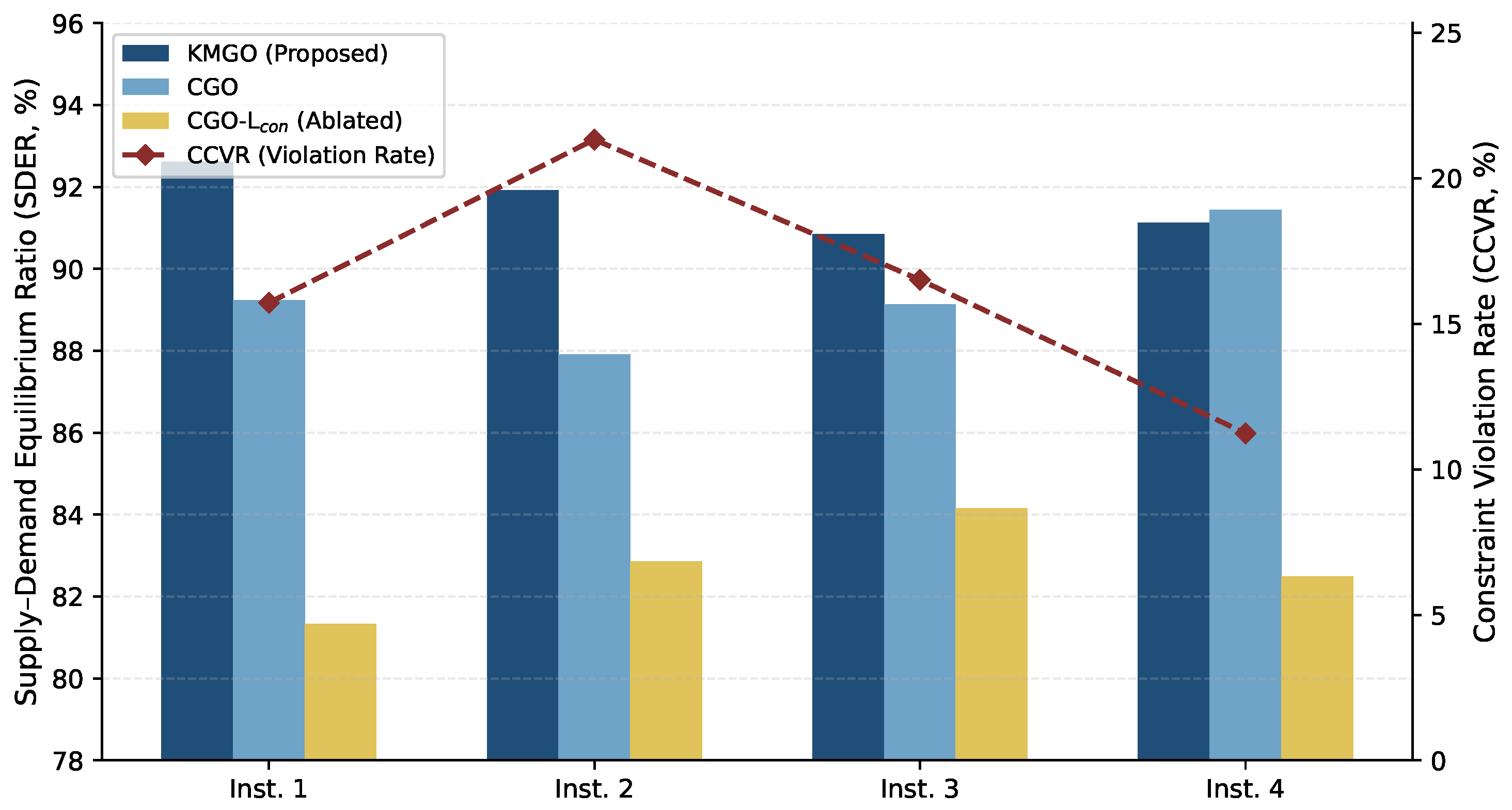
Table 8 compares KMGO and CGO with the KM reference in terms of idle distance, platform revenue, and passenger waiting time. The learned methods do not strictly dominate KM; instead, their values remain close to the reference across the reported instances. Lower idle distance and passenger waiting time are preferred, whereas higher platform revenue is preferred. The comparison supports the interpretation of the neural model as an approximation that trades small objective deviations for substantially lower online computation time. In addition to the instance-level comparison in Table 8, Figure 9 provides a complementary comparison with representative dispatching baselines under peak and off-peak conditions.
Table 8.
Objective function value analysis.
| Instance | Method | IdleDistance | PlatformRevenue | PassengerWaiting Time |
|---|---|---|---|---|
| 1 | KM | 4520 | 1283 | 903 |
| KMGO | 4671 | 1371 | 934 | |
| CGO | 4710 | 1278 | 958 | |
| 2 | KM | 5250 | 1431 | 955 |
| KMGO | 5349 | 1402 | 973 | |
| CGO | 5315 | 1387 | 959 | |
| 3 | KM | 6120 | 1652 | 1020 |
| KMGO | 6230 | 1569 | 1038 | |
| CGO | 6285 | 1569 | 1047 | |
| 4 | KM | 6221 | 1665 | 1037 |
| KMGO | 6214 | 1643 | 1036 | |
| CGO | 6236 | 1650 | 1042 | |
| 5 | KM | 7723 | 2069 | 1331 |
| KMGO | 7741 | 2023 | 1336 | |
| CGO | 7763 | 2088 | 1341 | |
| 6 | KM | 8109 | 2161 | 1329 |
| KMGO | 8238 | 2138 | 1350 | |
| CGO | 8182 | 2158 | 1335 | |
| 7 | KM | 9341 | 2413 | 1531 |
| KMGO | 9527 | 2377 | 1562 | |
| CGO | 9341 | 2413 | 1531 | |
| 8 | KM | 11233 | 3009 | 2340 |
| KMGO | 11187 | 2947 | 2326 | |
| CGO | 11225 | 2981 | 2335 |
The KM algorithm has polynomial complexity for standard assignment, but its runtime can still be substantial on the reported large instances. The learned model moves most computation to offline training and performs a forward pass during online dispatch. CGO further reduces dependence on KM-generated training labels by using the decision objective and constraint penalties.
As shown in Table 9, KM requires an average of 242.47 s per instance, whereas the proposed model requires 2.47 s. This corresponds to a 98.98% reduction in average online computation time, or approximately a 98.2-fold speedup. The result supports the use of the neural dispatcher as a seconds-level approximation for high-frequency operation; it does not imply millisecond-level latency or exponential KM complexity.
5.3. Transportation System Implications
The results suggest four implications for ride-hailing system design. First, prediction models should be assessed not only by MAE or RMSE, but also by how their outputs affect downstream allocation. Second, a trained neural dispatcher can act as a fast online approximation when repeatedly solving a reference optimizer is too slow for the decision frequency. Third, explicit capacity penalties are useful for discouraging regional over-allocation, as indicated by the CCVR ablation. Fourth, the three-city evaluation suggests adaptation potential across heterogeneous demand settings, but transfer to unseen cities still requires dedicated validation.
6. Conclusions
This study proposed a decision-focused end-to-end trainable framework for scalable vehicle dispatching in ride-hailing systems. The framework integrates multi-graph spatiotemporal demand representation with a recurrent Transformer-based dispatching module and incorporates constraint-aware loss terms to guide capacity-aware vehicle allocation. Experiments on three real-world ride-hailing datasets show competitive dispatching quality and zero CCVR for the proposed model in the reported city-level comparison. The model reduces average online computation time from 242.47 s for KM to 2.47 s, supporting its role as an efficient approximation for high-frequency operation. The prediction results also show that a dedicated forecasting model can achieve lower standalone error, reinforcing the decision-focused rather than prediction-dominance interpretation.
Limitations and future work. The present study uses grid-level distance and historical demand and does not model uncertainty, road-network travel time, battery state of charge, charging-station availability, energy consumption, or heterogeneous fleet constraints. It also evaluates logged multi-city datasets rather than an online simulator, digital twin, or field deployment, and it does not establish transfer performance on unseen cities. Future work should address these limitations through uncertainty-aware prediction, road-network and energy models, richer fleet constraints, and online closed-loop evaluation.
Author Contributions
Conceptualization, Y.G. and Y.Q.; methodology, Y.G. and Y.Q.; software, Y.G.; validation, Y.G. and H.W. (Haoran Wang); formal analysis, Y.G. and H.W. (Hongao Wang); investigation, Y.G.; resources, Y.Q.; data curation, Y.G. and H.W. (Hongao Wang); writing—original draft preparation, Y.G.; writing—review and editing, Y.Q. and H.W. (Haoran Wang); visualization, Y.G.; supervision, Y.Q.; project administration, Y.G. All authors have read and agreed to the published version of the manuscript.
Funding
This work was supported by the Natural Science Foundation of Zhejiang Province (grant number LMS25G010003) and the Scientific Research Project of Zhejiang Provincial Department of Education (grant number Y202454572).
Institutional Review Board Statement
Not applicable.
Informed Consent Statement
Not applicable.
Data Availability Statement
Data will be made available on request.
Acknowledgments
The authors acknowledge the support described in the Funding section.
Conflicts of Interest
The authors declare no conflicts of interest.
References
- Martínez-Díaz, M.; Soriguera, F. Autonomous vehicles: theoretical and practical challenges. Transportation Research Procedia 2018, 33, 275–282, XIII Conference on Transport Engineering, CIT2018. [Google Scholar] [CrossRef]
- Olayode, I.O.; Du, B.; Severino, A.; Campisi, T.; Alex, F.J. Systematic literature review on the applications, impacts, and public perceptions of autonomous vehicles in road transportation system. J. Traffic Transp. Eng. (English Edition) 2023, 10, 1037–1060. [Google Scholar] [CrossRef]
- Guo, Y.; Li, W.; Xiao, L.; Choudhary, A.; Allaoui, H. Enhancing efficiency and interpretability: A multi-objective dispatching strategy for autonomous service vehicles in ride-hailing. Comput. Ind. Eng. 2024, 194, 110385. [Google Scholar] [CrossRef]
- Al-Kanj, L.; Nascimento, J.; Powell, W.B. Approximate dynamic programming for planning a ride-hailing system using autonomous fleets of electric vehicles. Eur. J. Oper. Res. 2020, 284, 1088–1106. [Google Scholar] [CrossRef]
- Li, B.; Zhao, M.; Chen, N.; Li, Z.; Sun, H. The Ride-Hailing and Pricing Strategy Decision With the Application of Autonomous Vehicles. Manag. Decis. Econ. 2026, 47, 286–308. [Google Scholar] [CrossRef]
- Yue, X.; Liu, Y.; Shi, F.; Luo, S.; Zhong, C.; Lu, M.; Xu, Z. An End-to-End Reinforcement Learning Based Approach for Micro-View Order-Dispatching in Ride-Hailing. In Proceedings of the 33rd ACM International Conference on Information and Knowledge Management, New York, NY, USA, 2024; CIKM ’24. pp. 5054–5061. [Google Scholar] [CrossRef]
- Guo, Y.; Zhang, Y.; Yu, J.; Shen, X. A Spatiotemporal Thermo Guidance Based Real-Time Online Ride-Hailing Dispatch Framework. IEEE Access 2020, 8, 115063–115077. [Google Scholar] [CrossRef]
- Wen, D.; Li, Y.; Lau, F.C.M. A Survey of Machine Learning-Based Ride-Hailing Planning. IEEE Trans. Intell. Transp. Syst. 2024, 25, 4734–4753. [Google Scholar] [CrossRef]
- Ge, H.; Hu, X.; Cheng, M. DHDRDS: A Deep Reinforcement Learning-Based Ride-Hailing Dispatch System for Integrated Passenger–Parcel Transport. Sustainability 2025, 17. [Google Scholar] [CrossRef]
- Bertsimas, D.; Kallus, N. From Predictive to Prescriptive Analytics. Manag. Sci. 2020, 66, 1025–1044. [Google Scholar] [CrossRef]
- Yuan, E.; Chen, W.; Van Hentenryck, P. Reinforcement learning from optimization proxy for ride-hailing vehicle relocation. J. Artif. Intell. Res. 2022, 75, 985–1002. [Google Scholar] [CrossRef]
- Bao, Y.; Gao, J.; He, J.; Oliehoek, F.A.; Cats, O. Timing the Match: A Deep Reinforcement Learning Approach for Ride-Hailing and Ride-Pooling Services. arXiv 2025, arXiv:cs.LG/2503.13200. [Google Scholar]
- Yan, L.; Tang, R. Dual-Layer Optimization for Supply–Demand Balance in Urban Taxi Systems: Multi-Agent Reinforcement Learning with Dual-Attention Mechanisms. Electronics 2025, 14. [Google Scholar] [CrossRef]
- Elmachtoub, A.N.; Grigas, P. Smart “Predict, then Optimize”. Manag. Sci. 2022, 68, 9–26. [Google Scholar] [CrossRef]
- Sadeghi Eshkevari, S.; Tang, X.; Qin, Z.; Mei, J.; Zhang, C.; Meng, Q.; Xu, J. Reinforcement Learning in the Wild: Scalable RL Dispatching Algorithm Deployed in Ridehailing Marketplace. In Proceedings of the 28th ACM SIGKDD Conference on Knowledge Discovery and Data Mining, New York, NY, USA, 2022; KDD ’22. pp. 3838–3848. [Google Scholar] [CrossRef]
- Liu, Y.; Jia, R.; Ye, J.; Qu, X. How machine learning informs ride-hailing services: A survey. Commun. Transp. Res. 2022, 2, 100075. [Google Scholar] [CrossRef]
- Liu, Y.; Wu, F.; Lyu, C.; Li, S.; Ye, J.; Qu, X. Deep dispatching: A deep reinforcement learning approach for vehicle dispatching on online ride-hailing platform. Transp. Res. Part E Logist. Transp. Rev. 2022, 161, 102694. [Google Scholar] [CrossRef]
- Feng, J.; Gluzman, M.; Dai, J.G. Scalable Deep Reinforcement Learning for Ride-Hailing. In Proceedings of the 2021 American Control Conference (ACC), 2021; pp. 3743–3748. [Google Scholar] [CrossRef]
- Fan, Q.; van Essen, J.T.; Correia, G.H. A bi-level framework for heterogeneous fleet sizing of ride-hailing services considering an approximated mixed equilibrium between automated and non-automated traffic. Eur. J. Oper. Res. 2024, 315, 879–898. [Google Scholar] [CrossRef]
- Megantara, T.R.; Supian, S.; Chaerani, D.; Bon, A.T. The Application of the Piecewise Linear Method for Non-Linear Programming Problems in Ride-Hailing Assignment Based on Service Level, Driver Workload, and Fuel Consumption. Mathematics 2024, 12. [Google Scholar] [CrossRef]
- Guo, Y.; Zhu, R.; Li, W.; Boulaksil, Y.; Allaoui, H. Dynamic pick-up point recommendation with multi-modal deep forest and incentive-based adaptive Kuhn-Munkres Algorithm. Knowl.-Based Syst. 2025, 330, 114543. [Google Scholar] [CrossRef]
- van Engelen, M.; Cats, O.; Post, H.; Aardal, K. Enhancing flexible transport services with demand-anticipatory insertion heuristics. Transp. Res. Part E Logist. Transp. Rev. 2018, 110, 110–121. [Google Scholar] [CrossRef]
- Alonso-Mora, J.; Samaranayake, S.; Wallar, A.; Frazzoli, E.; Rus, D. On-demand high-capacity ride-sharing via dynamic trip-vehicle assignment. Proc. Natl. Acad. Sci. 2017, 114, 462–467. [Google Scholar] [CrossRef] [PubMed]
- Sayarshad, H.R.; Chow, J.Y. Non-myopic relocation of idle mobility-on-demand vehicles as a dynamic location-allocation-queueing problem. Transp. Res. Part E Logist. Transp. Rev. 2017, 106, 60–77. [Google Scholar] [CrossRef]
- Xu, Z.; Li, Z.; Guan, Q.; Zhang, D.; Li, Q.; Nan, J.; Liu, C.; Bian, W.; Ye, J. Large-Scale Order Dispatch in On-Demand Ride-Hailing Platforms: A Learning and Planning Approach. In Proceedings of the 24th ACM SIGKDD International Conference on Knowledge Discovery & Data Mining, New York, NY, USA, 2018; KDD ’18. pp. 905–913. [Google Scholar] [CrossRef]
- Sartori Vieira, F.; Sörensen, K.; Vanstenwegen, P. Optimization of a semiflexible demand-responsive feeder bus system using variable neighborhood search. Int. Trans. Oper. Res. 2025, 32, 3413–3440. [Google Scholar] [CrossRef]
- Feng, C.; Mei, Z. Optimization of Shared Autonomous Vehicles Routing Problem: From the View of Parking. Sustainability 2023, 15. [Google Scholar] [CrossRef]
- de Abreu Rodrigues, G.; Junqueira, L.; Vieira, J.G.V.; da Silva Júnior, O.S.; da Cunha, C.B. Rural last-mile distribution using a hybrid heuristic-multi-criteria decision-making framework. Expert Systems with Applications 2025, 289, 128331. [Google Scholar] [CrossRef]
- Benjelloun, R.; Tarik, M.; Jebari, K. Open Competency Optimization with Combinatorial Operators for the Dynamic Green Traveling Salesman Problem. Information 2025, 16. [Google Scholar] [CrossRef]
- Engelhardt, R.; Dandl, F.; Bogenberger, K. Speed-up Heuristic for an On-Demand Ride-Pooling Algorithm. arXiv 2020, arXiv:eess. [Google Scholar]
- Machado, B.; Pimentel, C.; de Sousa, A. Integration planning of freight deliveries into passenger bus networks: Exact and heuristic algorithms. Transp. Res. Part A Policy Pract. 2023, 171, 103645. [Google Scholar] [CrossRef]
- Kılıç, D.K.; Nielsen, P.; Miehe, F.; Yafrani, M.E. Trustworthiness analysis of heuristic routing algorithm with special constraints for autonomous vehicles in surveillance and coverage operations. Int. J. Syst. Sci. 2025, 56, 2717–2734. [Google Scholar] [CrossRef]
- Wu, Y.; Song, W.; Cao, Z.; Zhang, J.; Lim, A. Learning Improvement Heuristics for Solving Routing Problems. IEEE Trans. Neural Netw. Learn. Syst. 2022, 33, 5057–5069. [Google Scholar] [CrossRef] [PubMed]
- Thyssens, D.; Dernedde, T.; Sentanoe, W.; Schmidt-Thieme, L. On Distributional Dependent Performance of Classical and Neural Routing Solvers, 2025. arXiv arXiv:cs.LG/2508.02510.
- Latinopoulos, C.; Zavvos, E.; Kaklis, D.; Leemen, V.; Halatsis, A. Marine Voyage Optimization and Weather Routing with Deep Reinforcement Learning. J. Mar. Sci. Eng. 2025, 13. [Google Scholar] [CrossRef]
- Zhang, J.; Sun, Y.; Feng, Q.; Zhao, Y.; Wang, Z. Data-Driven Robust Optimization of the Vehicle Routing Problem with Uncertain Customers. Complexity 2022, 2022, 9064669. [Google Scholar] [CrossRef]
- Wang, X.; Li, N.; Jin, X. A Reinforcement Learning Hyper-Heuristic with Cumulative Rewards for Dual-Peak Time-Varying Network Optimization in Heterogeneous Multi-Trip Vehicle Routing. Algorithms 2025, 18. [Google Scholar] [CrossRef]
- Zhang, Y.; Long, Y.; Ni, Y.; Huang, L.; Wang, X.; Liu, J. Hierarchical Optimization via LLM-Guided Objective Evolution for Mobility-on-Demand Systems. arXiv 2025, arXiv:cs.AI/2510.10644. [Google Scholar]
- Zhang, H.; Wang, G.; Wang, X.; Zhou, Z.; Zhang, C.; Dong, Z.; Wang, Y. NondBREM: Nondeterministic Offline Reinforcement Learning for Large-Scale Order Dispatching. Proc. AAAI Conf. Artif. Intell. 2024, 38, 401–409. [Google Scholar] [CrossRef]
- Nejadshamsi, S.; Bentahar, J.; Wang, C.; Eicker, U. Predicting short-Term bike-Sharing demand at station level: A multi-Task dynamic graph-based spatiotemporal approach. Knowl.-Based Syst. 2026, 333, 114986. [Google Scholar] [CrossRef]
- Singh, A.; Al-Abbasi, A.O.; Aggarwal, V. A Distributed Model-Free Algorithm for Multi-Hop Ride-Sharing Using Deep Reinforcement Learning. IEEE Trans. Intell. Transp. Syst. 2022, 23, 8595–8605. [Google Scholar] [CrossRef]
- Guo, X.; Wang, Q.; Zhao, J. Data-Driven Vehicle Rebalancing With Predictive Prescriptions in the Ride-Hailing System. IEEE Open J. Intell. Transp. Syst. 2022, 3, 251–266. [Google Scholar] [CrossRef]
- Guo, Z.; Yu, B.; Shan, W.; Yao, B. Data-driven robust optimization for contextual vehicle rebalancing in on-demand ride services under demand uncertainty. Transp. Res. Part C Emerg. Technol. 2023, 154, 104244. [Google Scholar] [CrossRef]
- Kang, Y.; Li, T.; Zhao, L.; Gao, Z.; He, J.; Chen, Z.; Pu, B. Dual dynamic graph attention network driven deep reinforcement learning for flexible job-Shop scheduling. Knowl.-Based Syst. 2026, 335, 115192. [Google Scholar] [CrossRef]
- Liang, E.; Wen, K.; Lam, W.H.K.; Sumalee, A.; Zhong, R. An Integrated Reinforcement Learning and Centralized Programming Approach for Online Taxi Dispatching. IEEE Trans. Neural Netw. Learn. Syst. 2022, 33, 4742–4756. [Google Scholar] [CrossRef] [PubMed]
- Lin, K.; Zhao, R.; Xu, Z.; Zhou, J. Efficient Large-Scale Fleet Management via Multi-Agent Deep Reinforcement Learning. In Proceedings of the 24th ACM SIGKDD International Conference on Knowledge Discovery & Data Mining, New York, NY, USA, 2018; KDD ’18. pp. 1774–1783. [Google Scholar] [CrossRef]
- Yang, Y.; Luo, R.; Li, M.; Zhou, M.; Zhang, W.; Wang, J. Mean Field Multi-Agent Reinforcement Learning. In Proceedings of the 35th International Conference on Machine Learning, 10–15 Jul 2018; Dy, J., Krause, A., Eds.; PMLR, Proceedings of Machine Learning Research. Vol. 80, pp. 5571–5580. [Google Scholar]
- Wang, D.; Wang, Q.; Yin, Y.; Cheng, T. Optimization of ride-sharing with passenger transfer via deep reinforcement learning. Transp. Res. Part E Logist. Transp. Rev. 2023, 172, 103080. [Google Scholar] [CrossRef]
- Wang, Y.; Yin, H.; Wu, L.; Chen, T.; Liu, C. Secure Your Ride: Real-Time Matching Success Rate Prediction for Passenger-Driver Pairs. IEEE Trans. Knowl. Data Eng. 2023, 35, 3059–3071. [Google Scholar] [CrossRef]
- Kang, Y.; Chan, J.; Shao, W.; Salim, F.D.; Leckie, C. Long-Term Fairness in Ride-Hailing Platform. In Proceedings of the Machine Learning and Knowledge Discovery in Databases. Applied Data Science Track; Bifet, A., Krilavičius, T., Miliou, I., Nowaczyk, S., Eds.; Cham, 2024; pp. 223–239. [Google Scholar]
- Seo, Y.H.; Kim, D.K.; Kang, S.; Byon, Y.J.; Kho, S.Y. Rebalancing Docked Bicycle Sharing System with Approximate Dynamic Programming and Reinforcement Learning. J. Adv. Transp. 2022, 2022, 2780711. [Google Scholar] [CrossRef]
- Han, X.; Chong, Y.; Huangfu, Q. Shared Bicycle Scheduling Model Based on Price Incentive Mechanism. Math. Probl. Eng. 2018, 2018, 3713254. [Google Scholar] [CrossRef]
- Li, J.; Allan, V.H. Multiple Agents Dispatch via Batch Synchronous Actor Critic in Autonomous Mobility on Demand Systems. In Proceedings of the 16th International Conference on Agents and Artificial Intelligence (ICAART), 2024; Vol. 2, pp. 198–209. [Google Scholar] [CrossRef]
- Hiermann, G.; Schiffer, M. A decomposition-based approach for large-scale pickup and delivery problems. Eur. J. Oper. Res. 2026. [Google Scholar] [CrossRef]
- Wang, B.; Wang, Y.; He, X.; Hu, Y.; Yin, B. Multi-graph convolutional clustering network. IET Signal Process. 2022, 16, 650–661. [Google Scholar] [CrossRef]
- Zhang, B.; Niu, D.; Zhang, L.; Zhang, Q.; Li, Z. MSH-DTI: multi-graph convolution with self-supervised embedding and heterogeneous aggregation for drug-target interaction prediction. BMC Bioinform. 2024, 25, 275. [Google Scholar] [CrossRef] [PubMed]
- Devlin, J.; Chang, M.W.; Lee, K.; Toutanova, K. BERT: Pre-training of Deep Bidirectional Transformers for Language Understanding. In Proceedings of the 2019 Conference of the North American Chapter of the Association for Computational Linguistics: Human Language Technologies, Volume 1 (Long and Short Papers); Minneapolis, Minnesota, Jun 2019, Burstein, J., Doran, C., Solorio, T., Eds.; pp. 4171–4186. [CrossRef]
- Gan, Z.; Cheng, Y.; Kholy, A.; Li, L.; Liu, J.; Gao, J. Multi-step Reasoning via Recurrent Dual Attention for Visual Dialog. In Proceedings of the 57th Annual Meeting of the Association for Computational Linguistics; Florence, Italy, Jul 2019, Korhonen, A., Traum, D., Màrquez, L., Eds.; pp. 6463–6474. [CrossRef]
Figure 1.
Overall model architecture
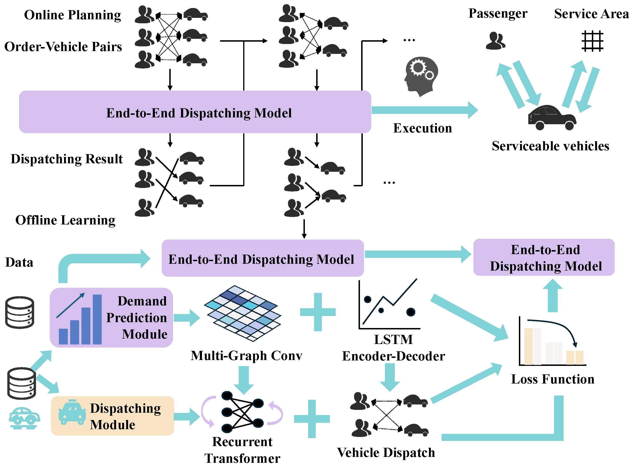
Figure 2.
Structure of the prediction module.
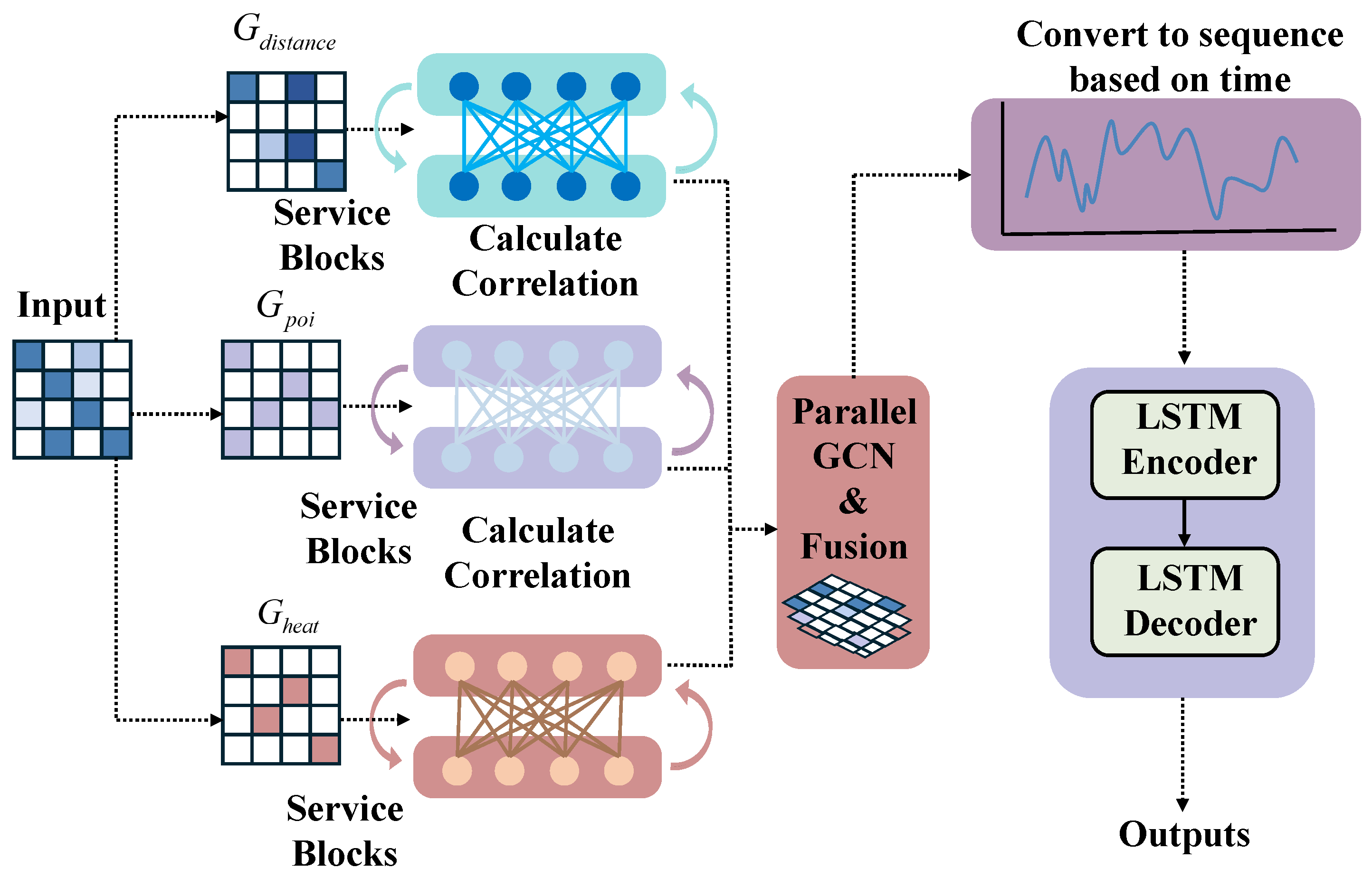
Figure 3.
Structure of the dispatching module.
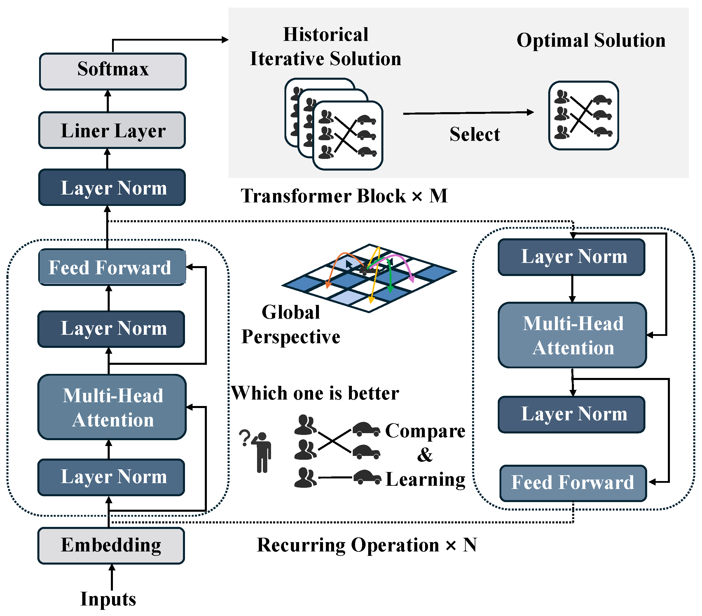
Figure 4.
Prediction error comparison across different models; lower values are better.
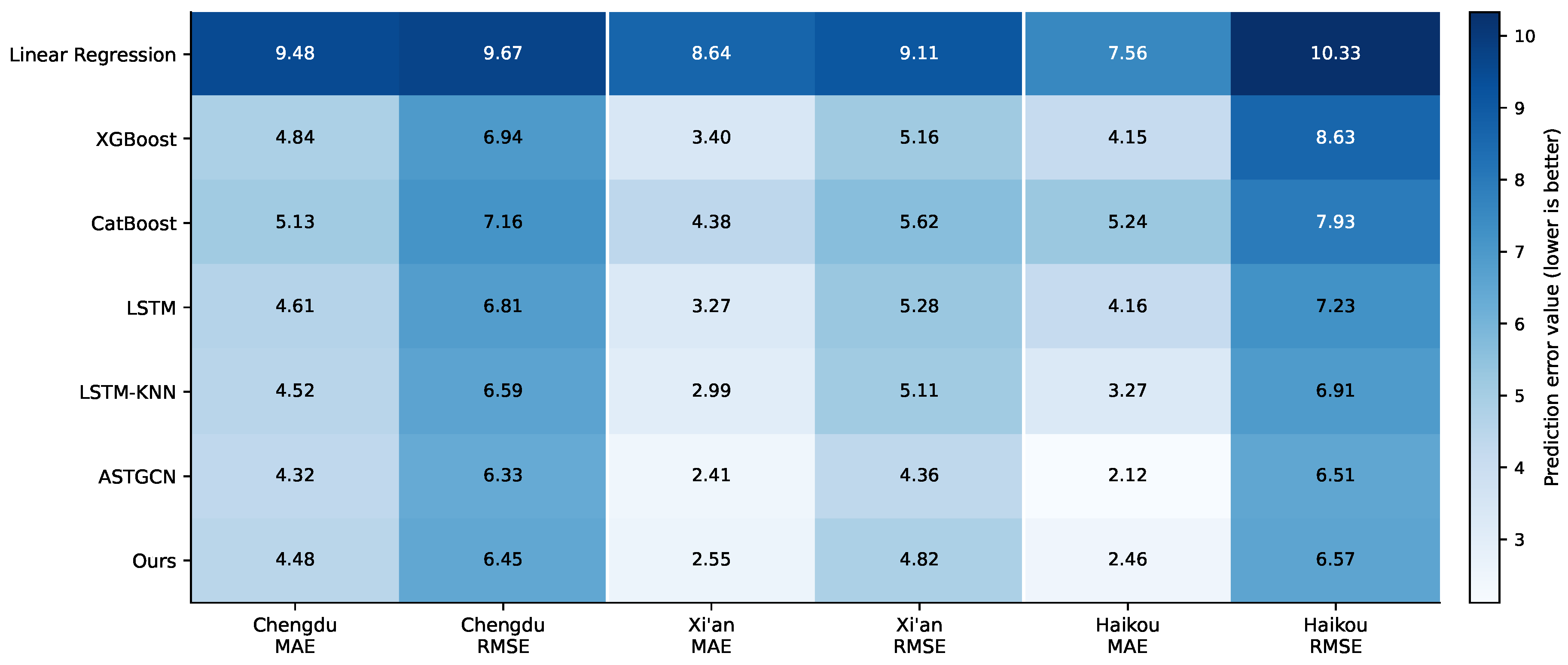
Figure 5.
Specific dispatching scenario demonstration.
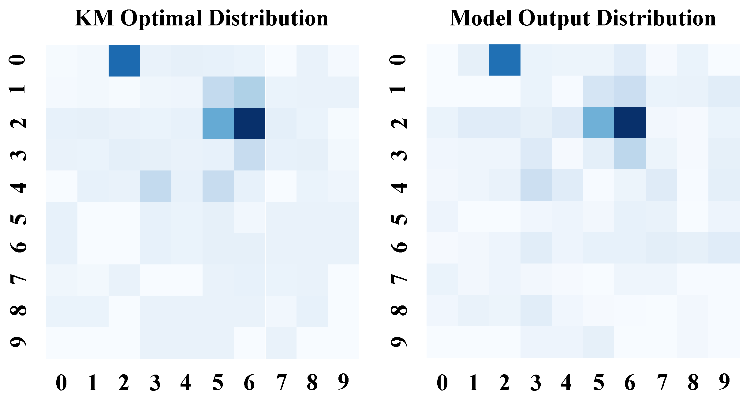
Figure 6.
Convergence trend of SDER and CCVR over training.
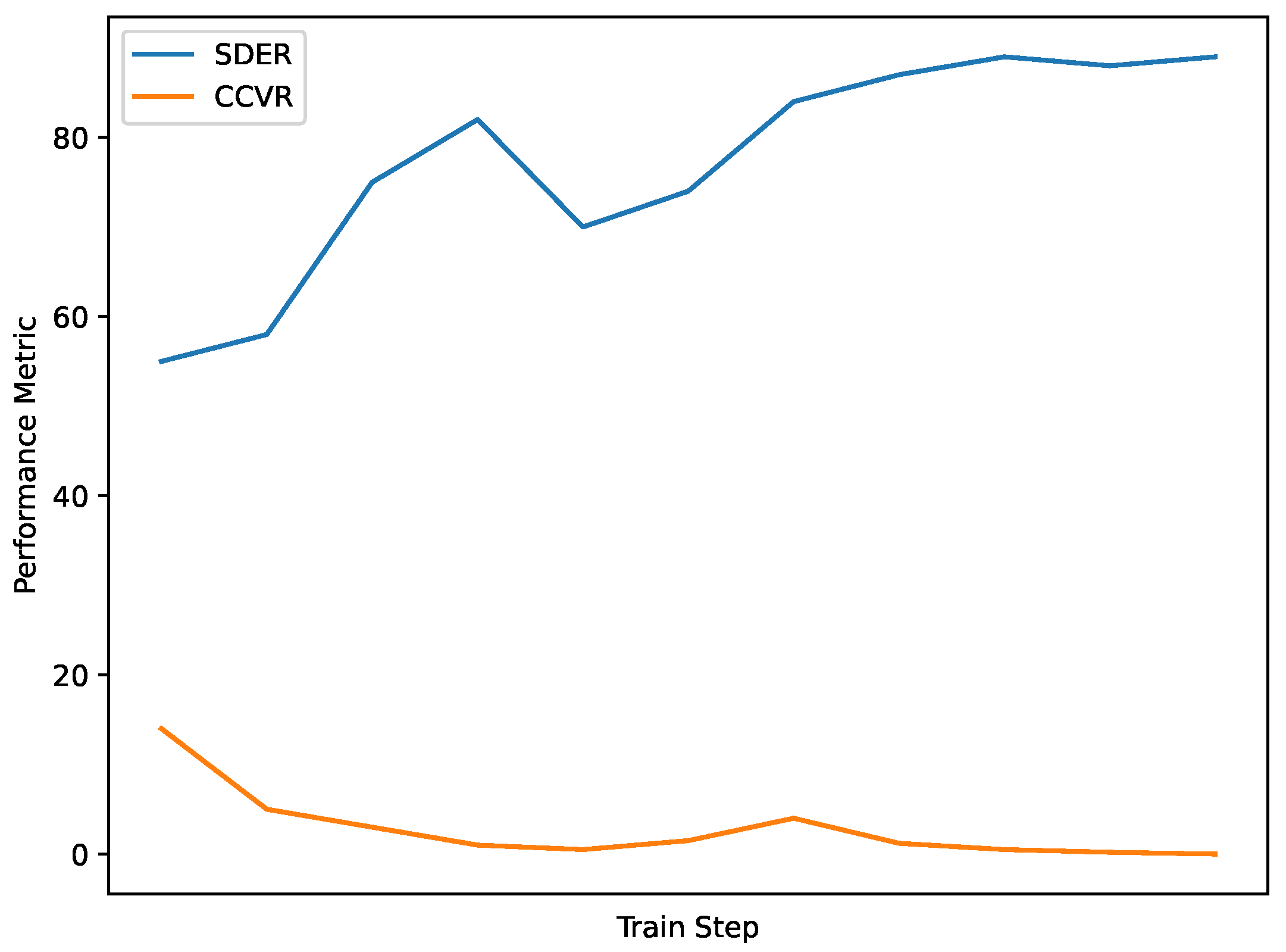
Figure 7.
Impact of removing positional encoding.
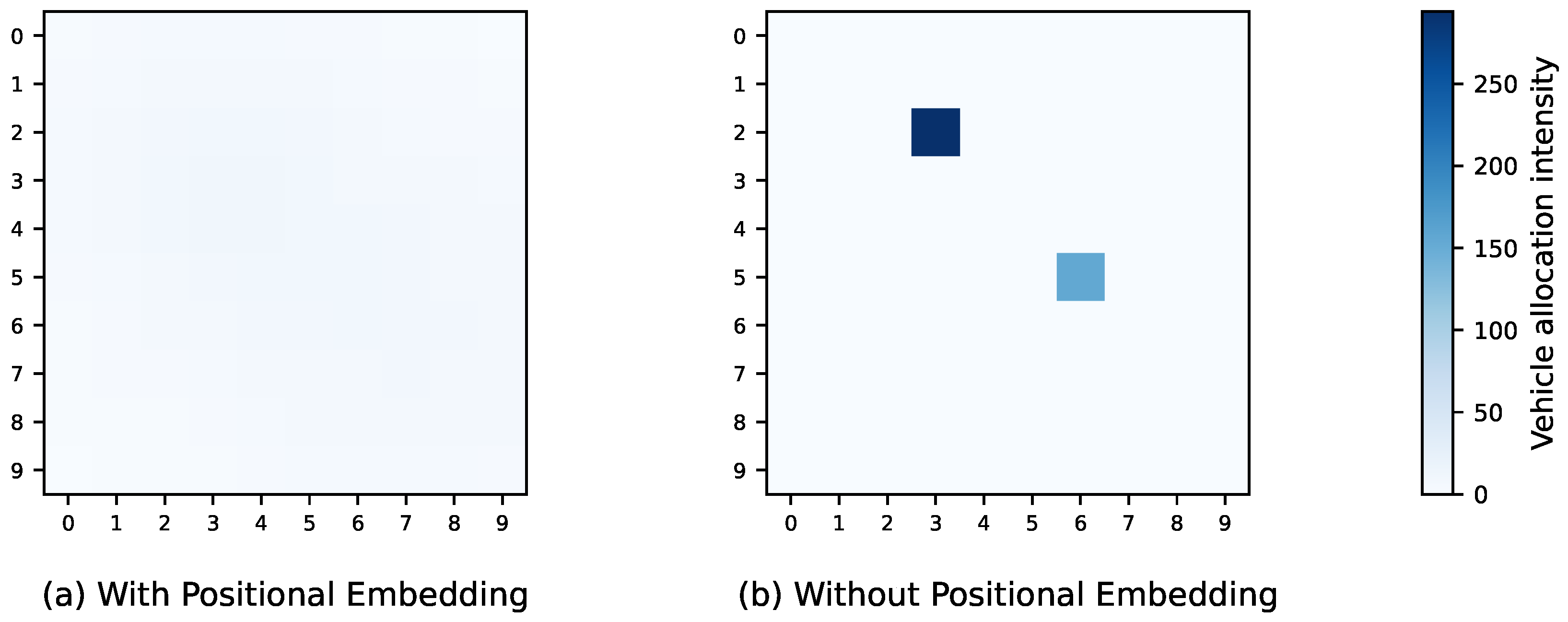
Figure 9.
Objectives function value comparison between peak and off-peak periods.
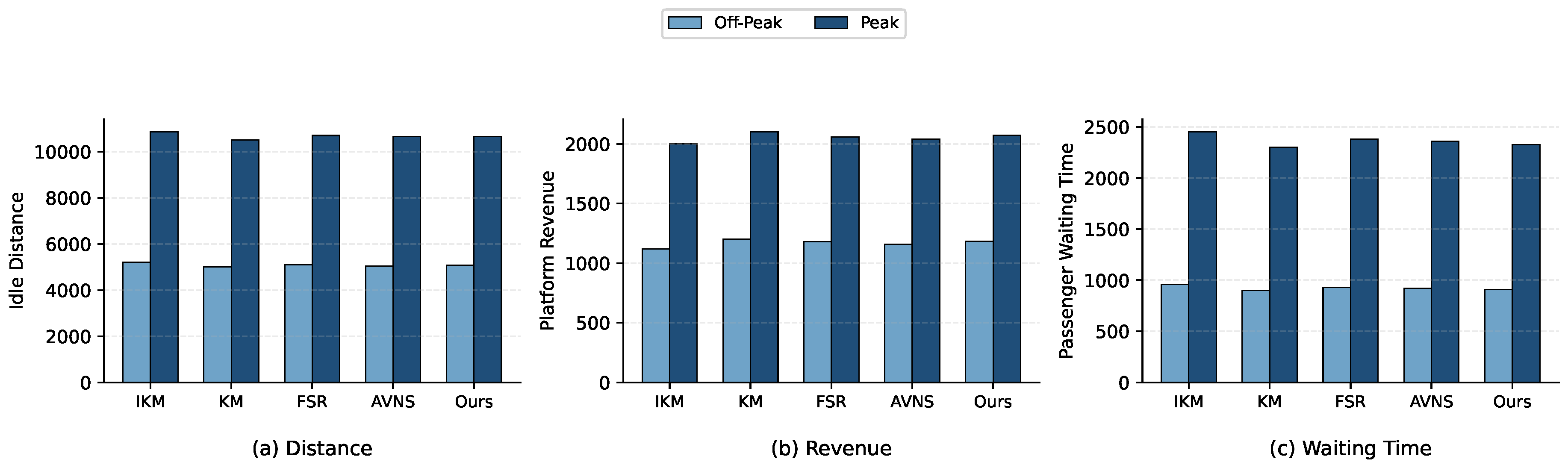
Table 1.
Existing research analysis.
| Research | Method | Scalability | Multi-Objective | Structure | Hetero. geneous |
|---|---|---|---|---|---|
| [22] | Heuristic | Medium | Yes | Pipeline | No |
| [23] | Heuristic + Optimization | Large | Yes | Pipeline | No |
| [24] | Heuristic | Medium | Yes | Pipeline | No |
| [26] | Heuristic (VNS) | Medium | Yes | Pipeline | No |
| [27] | Heuristic (VNS) | Medium | Yes | Pipeline | No |
| [28] | Heuristic + MCDM | Medium | Yes | Pipeline | Yes |
| [45] | Reinforcement Learning | Medium | Yes | Pipeline | No |
| [46] | Multi-Agent Reinforcement Learning | Medium | No | Pipeline | No |
| [25] | Learning + Planning | Large | Yes | Pipeline | Yes |
| [41] | Deep Reinforcement Learning | Medium | Yes | Pipeline | No |
| [42] | Data-Driven Optimization | Large | Yes | Pipeline | Yes |
| [43] | Robust Optimization | Large | Yes | Pipeline | Yes |
| [48] | Reinforcement Learning + Integer Programming | Large | Yes | Pipeline | Yes |
| [39] | Offline Reinforcement Learning | Large | Yes | End-to-End | Yes |
| [8] | Reinforcement Learning | Large | Yes | End-to-End | No |
| [51] | Reinforcement Learning | Medium | Yes | Pipeline | No |
| [52] | Regression + Heuristic | Medium | No | Pipeline | No |
| Ours | Deep Learning | Large | Yes | End-to-End | Yes |
Table 2.
Hyperparameter configuration.
| Parameter | Value |
|---|---|
| Optimizer | Adam |
| Learning rate | |
| Batch size | 32 |
| Total epochs | 500 |
| Transformer blocks (M) | 4 |
| Recursive steps (N) | 16 |
| 0.33 |
Table 3.
Prediction performance analysis across different models.
| Method | Chengdu | Xi’an | Haikou | |||
|---|---|---|---|---|---|---|
| MAE | RMSE | MAE | RMSE | MAE | RMSE | |
| Linear regression | 9.48 | 9.67 | 8.64 | 9.11 | 7.56 | 10.33 |
| XGBoost | 4.84 | 6.94 | 3.40 | 5.16 | 4.15 | 8.63 |
| CatBoost | 5.13 | 7.16 | 4.38 | 5.62 | 5.24 | 7.93 |
| LSTM | 4.61 | 6.81 | 3.27 | 5.28 | 4.16 | 7.23 |
| LSTM-KNN | 4.52 | 6.59 | 2.99 | 5.11 | 3.27 | 6.91 |
| ASTGCN | 4.32 | 6.33 | 2.41 | 4.36 | 2.12 | 6.51 |
| Ours | 4.48 | 6.45 | 2.55 | 4.82 | 2.46 | 6.57 |
Table 4.
Graph ablation experimental results.
| Ablation setting | MAE | RMSE |
|---|---|---|
| Full model (all graphs) | 2.46 | 6.57 |
| w/o distance-cost graph | 4.39 | 7.02 |
| w/o POI graph | 2.89 | 4.78 |
| w/o heat graph | 3.31 | 5.36 |
Table 5.
Dispatch performance comparison across methods and cities.
| Method | Chengdu | Xi’an | Haikou | |||
|---|---|---|---|---|---|---|
| SDER | CCVR | SDER | CCVR | SDER | CCVR | |
| KM | 78.48% | 1% | 79.53% | 0% | 81.42% | 4% |
| IKM | 82.35% | 0% | 84.65% | 0% | 85.36% | 1% |
| FSR | 93.12% | 0% | 94.71% | 0% | 91.38% | 0% |
| AVNS | 90.69% | 0% | 92.25% | 0% | 90.16% | 0% |
| Ours | 92.61% | 0% | 93.92% | 0% | 92.33% | 0% |
Table 9.
Running time analysis.
| Instance | Time (s) | |
|---|---|---|
| KM | Ours | |
| 1 | 85.53 | 1.81 |
| 2 | 115.32 | 2.85 |
| 3 | 180.41 | 2.72 |
| 4 | 502.51 | 4.33 |
| 5 | 287.09 | 2.21 |
| 6 | 181.16 | 1.95 |
| 7 | 115.44 | 1.98 |
| 8 | 278.10 | 2.32 |
| 9 | 180.70 | 1.14 |
| 10 | 252.44 | 2.36 |
| 11 | 236.81 | 2.62 |
| 12 | 494.13 | 3.16 |
| Average | 242.47 | 2.47 |
Disclaimer/Publisher’s Note: The statements, opinions and data contained in all publications are solely those of the individual author(s) and contributor(s) and not of MDPI and/or the editor(s). MDPI and/or the editor(s) disclaim responsibility for any injury to people or property resulting from any ideas, methods, instructions or products referred to in the content. |
© 2026 by the authors. Licensee MDPI, Basel, Switzerland. This article is an open access article distributed under the terms and conditions of the Creative Commons Attribution (CC BY) license (http://creativecommons.org/licenses/by/4.0/).
Copyright: This open access article is published under a Creative Commons CC BY 4.0 license, which permit the free download, distribution, and reuse, provided that the author and preprint are cited in any reuse.