

Submitted:
29 September 2026
Posted:
30 September 2026
You are already at the latest version
Abstract
Accurate prediction of the rainy-season onset is crucial for many in Southeast Africa. This paper explores the application of the Random Forest (RF) machine learning method to forecast the start of the October-November-December (OND) rainy season across the region. Our RF model was trained to predict onset dates using historical precipitation data, observations and forecasts of key climate drivers, such as the El Niño-Southern Oscillation (ENSO) and the Indian Ocean Dipole (IOD), and onset forecasts derived from dynamical seasonal forecast models. Comparing our RF model with the widely used ECMWF System 5.1 dynamical forecast showed improvements of 2-15 days in RMSE, particularly for forecast initialised in August-September, and CRPSS gains of up to +0.15 for individual countries for the same start dates. The results demonstrate that our RF model captures regional variability in onset timing and consistently outperforms climatology. Notably, predictions for the 2023 and 2024 rainy seasons reveal significant shifts driven by ENSO phase transitions. This study highlights the robustness of our RF approach in dealing with complex climate variables and underscores the potential for improving seasonal rainfall forecasts in the region, helping stakeholders make more informed decisions based on these forecasts.
Keywords:
Random Forest
; rainy season onset
; seasonal forecasting
; East Africa
; machine learning
; climate services
1. Introduction
The onset of the rainy season is a key climate event in Southeast Africa with implications for rainfed agriculture, water management, power production and disaster preparedness. Forecast information is particularly valuable when it indicates the likely timing of seasonal rains which is crucial for mitigating the adverse impacts of delayed or erratic rainfall. However, predicting the onset of the rainy season remains a challenging task due to the complex interplay of atmospheric, oceanic, and land-surface processes that influence regional climate patterns (Roy et al., 2023; Palmer et al., 2023; Roy and Troccoli, 2024).
In recent years, advancements in machine learning and data-driven approaches have opened new possibilities for improving the skill of seasonal forecasts. The Random Forest (RF) method, a widely used machine learning algorithm (Breiman, 2001), has shown great potential in handling the complexity of climate data, especially when trained on large amount of data, as demonstrated by Gibson et al. (2021), where RF achieved skill on par with dynamical models and offered interpretable insights into physical drivers.
This study develops gridded forecasts of the October-November-December (OND) rainy season in Southeast Africa, covering the countries of Tanzania, Malawi, Mozambique, Rwanda, and Zimbabwe, with a focus on Tanzania, through close collaboration with the Tanzania Meteorological Authority (TMA), as part of the 4-year EU-funded FOCUS-Africa project. These countries were selected because they formed the core geographical focus of the FOCUS-Africa activities, and a regular rectangular study domain was adopted to encompass them consistently. While the analysis presented here focuses on this domain, the methodology is generic and can readily be extended to neighbouring countries and regions, including Kenya and Ethiopia. TMA’s local expertise significantly informed both current methods for onset calculation and stakeholder requirements for forecast applications.
Two internally consistent data systems were constructed: one based on Multi-Source Weighted-Ensemble Precipitation (MSWEP) (Beck et al., 2019) and one based on Climate Hazards Group InfraRed Precipitation with Stations (CHIRPS) (Funk et al., 2015). For consistency, the same precipitation dataset was used to derive both the onset target and the associated lagged-rainfall predictors. These local inputs were combined with observed and forecast ENSO and IOD indices and with the dynamical seasonal onset forecasts. ENSO and the IOD were included because they are major large-scale drivers of OND rainfall variability and onset timing in Southeast Africa. ENSO can alter the Walker circulation and regional moisture transport, while the east–west sea-surface-temperature gradient associated with the IOD influences convection over the western Indian Ocean and East Africa. These relationships are season-, location-, and lead-time-dependent rather than deterministic (Wenhaji Ndomeni et al., 2018; Kolstad and MacLeod, 2022; Roy and Troccoli, 2024). Observed indices describe the large-scale state at forecast issue time, whereas forecast indices describe its expected evolution during the lead-up to OND. Their inclusion is therefore physically motivated but does not imply a causal interpretation of RF predictor importance.
Building on previous work (Zampieri et al., 2023; Roy et al., 2023), this study evaluates whether statistical post-processing can add useful information to dynamical seasonal onset forecasts across different initialization months.
The accumulated-anomalies method, proposed by Zampieri et al. 2023, is used here to create a more generic onset metric that can be applied across larger regions and different domains than the threshold-based method currently used by local institutions such as TMA. By comparing the model’s predictions for the 2023 and 2024 rainy seasons against ECMWF system 5.1 (s5.1) dynamical forecast systems, the study demonstrates the potential of the RF method to support decision-making in climate-sensitive sectors across Southeast Africa. ECMWF s5.1 was chosen as the primary baseline because multiple independent evaluations have shown that, among Copernicus seasonal forecast systems, ECMWF generally provides the highest precipitation forecast skill for East and Southern Africa, outperforming DWD and CMCC in terms of monthly anomaly correlations, predictive capability for the OND rains, and operational use across the region (Gebrechorkos et al., 2022; Tefera et al., 2025; Endris et al., 2021). As our RF model incorporates dynamical-model onset forecasts, including ECMWF-derived information, this comparison should be interpreted as an assessment of statistical post-processing relative to a raw dynamical forecast, rather than as a comparison between two fully independent forecasting systems.
2. Data and Methods
Two precipitation products were used to construct parallel historical datasets of the OND rainy-season onset: MSWEP and CHIRPS. The two products were not merged into a single training dataset. Instead, each product defined an internally consistent system: onset dates were derived from that product and its corresponding antecedent-rainfall predictors were calculated from the same product. Together, these provided two independent training datasets based on robust daily precipitation estimates. A comprehensive assessment of available precipitation datasets was carried out as part of FOCUS-Africa, identifying these as preferred options for Tanzania, owing to their long, spatially complete precipitation records and suitability for gridded onset estimation (Mliwa et al., 2025, in press). The characteristics and preprocessing of each dataset are described below.
MSWEP provides global precipitation estimates with a 0.1° resolution and three-hourly temporal resolution, combining satellite data, ground station measurements, and reanalysis products. It offers high temporal frequency (3-hourly data), making it ideal for hydrological applications (Beck et al., 2019). It was used both to provide MSWEP-based onset dates and to calculate the corresponding lagged-rainfall predictors.
CHIRPS, a high-resolution (0.05° grid) dataset, is designed for drought monitoring and combines satellite-derived estimates with ground station data. It provides daily rainfall estimates, particularly useful for regions with sparse observational networks like Southeast Africa (Funk et al., 2015). For this study, the regridded version of CHIRPS available at 0.25° resolution was chosen for computational purposes. The MSWEP data were then bilinear interpolated onto the CHIRPS grid, resulting in a common 0.25° grid spanning 27.875° S–0.125° S and 24.125° E–40.875° E. Dynamical seasonal forecast inputs were subsequently interpolated onto the same grid, with the same method, before model training and evaluation.
For each precipitation product, historical OND rainy season onset dates were calculated independently for every grid point and year. These were calculated as proposed by Zampieri et al. (2023) by identifying the point at which accumulated daily precipitation anomalies, calculated from the first of July, reached their minimum before a sustained period of above-average rainfall began. The climatology was defined as the mean daily rainfall from 1 July to 15 January, with reference to the 1993-2016 hindcast period. Formally the daily anomaly was calculated as:
αt = Pt − Pc
Where Pt is daily precipitation and Pc is the climatological daily mean. The accumulated anomaly from 1st of July was then calculated as:
Where At is the accumulated precipitation anomaly on day t and as is the daily precipitation anomaly on each day (s) from 1st of July to day t.
To account for the bimodal rainfall regime present in parts of the study area, particularly in northern Tanzania, the method was adapted. In these zones, an initial increase in accumulated daily rainfall anomalies was accepted as the onset if it resulted in a local maximum that exceeded the subsequent minimum by more than 40 mm, thus recognising the occurrence of an early, distinct rainy season, even if another rainfall minimum followed. The 40 mm separation criterion was part of the locally informed onset definition adopted for this study and was applied consistently at every grid point and for every year, rather than fitted separately by location or forecast start month. This approach identifies a distinct early wet period rather than automatically assigning onset to the later minimum. This method was chosen instead of onset estimation methods based on fixed daily-precipitation thresholds, as such methods are typically tailored to specific countries or areas and might not perform consistently across domains as large as the one considered here. Figure 1 shows an example of the onset calculation for the year 1997 from a randomly selected grid point.
Our RF model used 23 predictors, drawn from two main sources: observational data and dynamical forecast data (Table 1). With the data being retrieved from Copernicus Data Store (CDS), National Oceanic and Atmospheric Administration (NOAA), International Research Institute for Climate and Society (IRI) and GloH2O.
The observational predictors were restricted to information available before each forecast initialization date. They include ENSO 3.4 index (sea surface temperature, SST, anomalies in the central Pacific) and the Indian Ocean Dipole (IOD) index, which reflects SST anomalies across the Indian Ocean. The ENSO 3.4 was used with a lags of 1-3 months prior to forecast initialization and IOD with lags of 1-4 months. Forecast ENSO and IOD predictors represent information available at the forecast issue date about the expected evolution of large-scale sea-surface-temperature conditions before and during the OND season. For a forecast initialised in month m, fc_L1, fc_L2, and fc_L3 denote the ensemble-mean index forecasts for the first, second, and third months following that initialisation, respectively. Observed and forecast indices have complementary roles: observed lags describe the realised large-scale climate state before forecast initialisation, whereas forecast indices describe the modelled evolution of that state into the forthcoming months. Since they may be correlated, their inclusion does not assume that they provide independent information. Rather, our RF is allowed to use either or both sources of information where this improves out-of-sample prediction; their importance is not interpreted as a causal effect. In addition, local precipitation predictors derived from MSWEP or CHIRPS with lags of 1-3 months were included to capture local rainfall variability. The rainfall predictors followed the parallel-data-system approach: MSWEP monthly averages were used when the onset was calculated from MSWEP daily accumulated anomalies and CHIRPS was used similarly for CHIRPS-based onset estimates.
The forecast data used as predictors in our RF model consisted of onset forecasts from three distinct dynamical seasonal forecast systems: the European Centre for Medium-Range Weather Forecasts (ECMWF) system 5.1 (s5.1), the Deutscher Wetterdienst (DWD) s2.1, and the Centro Euro-Mediterraneo sui Cambiamenti Climatici (CMCC) s3.5. For each forecast system, the predicted onset of the rainy season was derived using the same accumulated rainfall anomaly method applied to the observational target. Forecasts from individual ensemble members were aggregated by calculating the mean predicted onset date, which was then used as a predictor in our RF model. Figure 2 shows an example forecast of accumulated daily anomalies from the ECMWF s5.1, with predicted onset dates from individual members marked by green circles and the ensemble-mean onset, used as a predictor, indicated as a dashed vertical line. Combined, these predictors allowed our RF to function as a statistical post-processing system that augments dynamical model forecasts using observational information, rather than as an entirely independent forecast system.
In addition to the forecasts of onset, forecasts of ENSO3.4 and IOD were also generated from SST forecasts from the required domains. These indices were calculated for lead times of 1-5 months for all initialization dates, first by averaging across all ensemble members for each model, and then by averaging across models.
The RF model was chosen as the ML model for this study, after comparison with Bayesian Ridge and multilayer perceptron models under the common-predictor leave-one-year-out hindcast framework; it was not assumed a priori to be the most skilful method in every setting. Furthermore, it was chosen due to its ability to handle complex datasets with numerous predictors. The RF model generates multiple decision trees during training, each providing a prediction. The final output is an ensemble of all individual tree predictions, ensuring a probabilistic forecast that reflects its uncertainty and can capture non-linear relationships between the predictors.
Our RF model was trained at each of the 7616 grid points over the whole study domain. Separate RF models were trained at each grid point. Each model contained 250 trees and used squared-error reduction as the tree-splitting criterion. Testing over 1/8th of the grid showed no significant skill improvement at 500 trees and a degradation at 100 trees. To reduce overfitting with the limited number of historical years, the forest was regularised by limiting tree depth, requiring a minimum number of samples in terminal nodes, randomly sub-sampling predictors at each split, and drawing each tree from a sub-sample of the training data. Candidate configurations were evaluated using nested leave-one-year-out temporal tuning, with the outer held-out year excluded from both hyperparameter selection and final evaluation. The selected reference configuration used a maximum tree depth of 4, a minimum split size of 6, a minimum leaf size of 2, square-root predictor sub-sampling and a bootstrap sample fraction of 0.63. Hyperparameter selection was based on optimizing CRPS relative to the leave-one-year-out climatological reference and average over the individual tests.
Probabilistic forecasts were derived by ranking the predictions of all decision trees at each grid point, and defining tercile thresholds (33rd and 67th percentiles) to represent the probability of onset dates being below-normal, normal, and above-normal. The computational environment included Python (3.7; Van Rossum and Drake 2009), scikit-learn (1.4; Pedregosa et al. 2011), and parallelized computations on an online cluster. Generative artificial intelligence was used to assist with adjusting python code for figure generation (Figure 3, Figure 4, Figure 5, Figure 6, Figure 7 and Figure 8).
The models were trained in a leave-one-out framework over the 24-year training period (1993-2016). For each target year, the model was trained using predictors and onset dates for the remaining 23 years. Hyperparameter selection was performed only within those 23 training years using a nested year-wise cross-validation procedure. The average across year configuration with the highest skill was then used to predict the held-out year. This procedure produced 24 out-of-sample forecasts for each evaluated initialization month. Model skill was evaluated with this nested leave-one-year-out hindcast dataset.
Hindcast skill claims are based on the 1993–2016 leave-one-year-out evaluation, meaning that each target year is temporally out of sample. However, the outer folds share much of their training data and should not be interpreted as independent development and validation datasets. The reported scores instead summarize the complete set of year-wise out-of-sample hindcasts over 1993–2016. The 2023 and 2024 forecasts are presented only as operational case studies.
To test whether the choice of RF was justified, the RF was compared with Bayesian Ridge and multilayer perceptron (MLP) models. All methods used the same leave-one-year-out setup, target variable, grid point mask and verification metrics. The comparison was undertaken using the same predictors. RF uncertainty was represented by the distribution of individual-tree predictions; Bayesian Ridge and MLP predictive distributions were represented using their fitted mean and residual uncertainty. Performance was assessed using CRPS and CRPSS relative to the leave-one-year-out climatological reference. The comparison therefore evaluates the sensitivity of forecast skill to algorithm choice under identical predictor information, rather than identifying a universally optimal model.
3. Results
We assess the forecast performance in three stages. First, we compare the ML methods under a common predictor set and identical leave-one-year-out method. This establishes whether the choice of RF is supported by skill. Second, we evaluate our RF forecast against the raw ECMWF dynamical onset forecast to quantify the added value of statistical post-processing. Finally, we examine the spatial distribution of skill at the country level and illustrate forecast behaviour for recent operational case-study years.
Figure 3 shows positive CRPSS for all three evaluated methods at all four forecast initialisations. The MLP attains the highest Tanzania-average skill for the June, July, and August initialisations (CRPSS of 0.087, 0.095, and 0.122, respectively), while RF has the highest score for the September initialisation (0.114). RF skill is close to that of the other methods in July and August and remains positive from June onwards. Thus, the comparison does not suggest that RF is universally the most skilful method. Its use as the operational reference reflects a combination of competitive skill over Tanzania, stable behaviour across forecast start months, direct ensemble-based probabilistic output, and the possibility of examining the influence of different predictor groups.
We next assess whether RF post-processing provides deterministic added value relative to the raw ECMWF s5.1 onset forecast. This comparison enables the calculation of RMSE for both systems and assess the potential improvement of the RF model over ECMWF forecasts. RMSE was calculated from the ensemble-mean onset forecast and the observed onset date. Figure 4 shows an example of the average difference in RMSE for forecasts initialised in July, averaged over all years. Table 2 shows the RMSE difference between our RF model and ECMWF forecasts for onset date across six countries in Southeast Africa.
Overall, our RF model demonstrates the greatest improvements in Malawi, particularly in August (-7 days) and September (-15 days), and in Mozambique, where the largest reductions occur in July (-7 days) and September (-13 days). Tanzania also shows substantial gains, with errors reduced by 7 days in August and 12 days in September similarly to Zimbabwe that shows errors reduced by –5 in August and –10 in September. Burundi shows modest improvements in July (-3 days) and August (-2 days), but substantial improvements in September (-9 days). By contrast, Rwanda shows little to no improvement, or slight deterioration, with differences of 0–3 days across all months. It is worth noting, however, that Rwanda, and Burundi, have much smaller spatial coverage than the other countries considered.
Seasonally, the strongest improvements are observed in late-season forecasts (August–September), especially in Malawi, Mozambique, and Tanzania. Early-season results (June–July) are, as expected, more mixed due to the longer lead times, with improvements in Malawi and Mozambique, but smaller deteriorations in other countries.
For operational implementation, our RF predictive distribution was represented by 51 tree predictions sampled from the 250-tree forest, matching the 51-member ensemble size of the real-time ECMWF s5.1 seasonal forecast. The historical ECMWF reforecasts available for the 1993–2016 hindcast period contain 25 members; all available members were retained for the hindcast evaluation.
Skill was measured using the Continuous Ranked Probability Score (CRPS) (Hersbach, 2000) and its skill score, CRPSS. For a predictive CDF F and observed value y.
With the skill score defined as:
Here, the reference forecast used to compute the CRPS_ref is the climatological distribution over the years 1993 to 2016. Positive CRPSS values indicate that the RF model outperforms climatology, while negative indicates deterioration. Our RF model’s performance against climatology was compared to the onset forecast derived from the ECMWF s5.1 dynamical forecasting system performance against the same climatology. Figure 5 shows improvements in CRPSS for forecasts initialised in July, with the largest improvements over the north-eastern part of the domain, especially over Tanzania. Table 3 presents the spatially aggregated differences in Continuous Ranked Probability Skill Score (CRPSS) between our RF model and ECMWF forecasts for onset prediction. Positive values indicate an improvement in forecast skill by our RF model relative to ECMWF.
Table 3 shows the aggregated CRPSS improvements across all countries. A positive RF–ECMWF difference does not necessarily imply positive absolute RF skill relative to climatology, because it can occur when both systems have negative CRPSS but RF has the less negative score. Our RF model generally demonstrates small but consistent improvements, with the largest gains observed in Tanzania (up to +0.15 in August and +0.14 in September) and Burundi (+0.09 in September). Mozambique also see small improvements of +0.02 to +0.05 across all months. Malawi shows only modest increases (+0.01 to +0.04), while Rwanda presents mixed results: small positive improvements in June, July and September, but a notable decline (-0.08) in August. Finally, Zimbabwe shows a similar small improvement for all month (+0.04 to +0.06). Formal significance testing was not undertaken because the number of hindcast years is limited and the data are spatially correlated; the results should therefore be interpreted as indicative differences in predictive performance.
Similarly to the improvements for RMSE, the strongest improvements in CRPSS occur in late-season months (August-September), particularly in Tanzania and Burundi. In contrast, early-season months (June-July) show smaller but consistent skill increases across most countries with exception of Tanzania which for all months see the largest improvements of all the countries.
After running operationally each month as part of the FOCUS-Africa project since early 2023, the model has produced forecasts for two OND seasons, illustrating the range of spatial onset-anomaly patterns represented by the operational product. This is seen in Figure 6, which shows the MSWEP-based forecasts from July of each year alongside the observations. These indicated relatively contrasting large-scale spatial features, with later onset in the southern parts of the domain and earlier onset in the northern regions in 2023, and a reverse pattern in 2024. In both cases, the forecasts reproduce several of the large-scale spatial anomaly patterns seen in the corresponding observations and the estimated actual onset dates from the MSWEP dataset, which displays dipole-like patterns (Figure 7). These two operational cases are illustrative only and, because they cover just two years, do not establish forecast robustness; quantitative performance is evaluated using the 1993–2016 leave-one-year-out hindcasts.
Notably, these forecasts were initialised as early as July 2023 and July 2024, respectively, several months before the OND season. The spatially coherent patterns shown in the July forecasts (Figure 6) and corresponding observations (Figure 7) suggest that large-scale conditions, including ENSO and the IOD, may have contributed to the onset variability observed in these two years. This highlights the potential for useful predictive value several months before the rainy season begins. In fact the dipole-like pattern was evident in all subsequent forecasts issued during both years.
Our RF model’s capability to rank predictors based on their importance provides insights into the factors associated with the onset of the rainy season. Analysis of variable importance reveals that global climate drivers such as ENSO and IOD indices together with local observations make the largest contribution to predictive skill at longer lead times (i.e., June, but also July). As the rainy season approaches (namely in August and September), dynamical model outputs (for all three ECMWF, DWD and CMCC systems) increase their relevance likely due to their ability to capture evolving regional-scale patterns and local atmospheric conditions relevant to onset timing (Figure 8).
4. Discussion and Conclusions
This study demonstrates that statistical post-processing using RF can improve predictions of OND rainy-season onset across much of Southeast Africa relative to raw dynamical forecasts. However, some limitations should be considered when interpreting these results. The 1993–2016 evaluation contains 24 target years, leaving 23 years for model fitting within each leave-one-year-out fold. This period was the longest common hindcast period for which the onset target and predictors from all the dynamical forecasting systems were consistently available. RF complexity was therefore constrained through the nested temporal tuning procedure, and the results should be interpreted as evidence of skill over this specific hindcast period rather than proof of universally robust performance. The many spatial grid points do not constitute additional independent temporal samples, because onset anomalies are spatially correlated. Evaluation over additional independent years, using predictors available in real time, will be required to establish the stability of the system under future climate conditions.
While our RF model performed well across most of the study area, certain local areas, such as western Zimbabwe, exhibited lower skill. This may be due to local climatic complexity and/or data sparsity. Future improvements could include incorporating additional local predictors such as soil moisture, vegetation indices, while the inclusion of sub-seasonal forecasts represents another promising direction for future research. Further increasing the resolution of observational datasets could also help make the model more relevant to the end-users. Furthermore, the definition of an OND onset season used is tailored to Tanzania, reflecting its bimodal and unimodal rainfall regimes. This may partly explain the larger skill improvements observed there compared to other countries. This underscores the need for continued stakeholder engagement and collaboration with local meteorological agencies to refine model definitions and enhance operational relevance.
Improved understanding of the physical mechanisms linking ENSO and IOD to regional rainfall variability could further enhance model performance. This could include exploring additional lead or lag times for some predictors over certain areas, and may also help anticipate how future climate change-driven shifts in these large-scale drivers might affect seasonal rainfall patterns.
In this study, RF is not assumed a priori to be the most skilful machine learning method. It was selected following a comparison with Bayesian Ridge and multilayer perceptron models under the same leave-one-year-out hindcast framework and common predictors. Although MLP achieved higher skill in some start months, RF was retained as the main model because it exhibited more consistent performance across all start months, it provides an ensemble-based probabilistic forecast directly and its behaviour can be easily analysed through its predictor-importance diagnostics.
Our RF model’s ability to integrate multiple predictors—including observational indicators and outputs from dynamical forecast models—led to an improvement over ECMWF’s s5.1 dynamical forecasts across much of the study region, particularly for August-September forecasts, confirming its potential as a powerful tool for operational forecasting. Utilizing forecasts from multiple dynamical models provided complementary information and may have allowed the RF approach to leverage the strengths from different systems across different areas of the domain, contributing to improved predictive performance.
Our RF model achieved measurable improvements in prediction accuracy, with notable regional differences that may partly reflect the influence of large-scale climate drivers such as ENSO and IOD. In particular, our RF model captured contrasting north-south onset dipole patterns in 2023 and 2024 that were associated with differing large-scale climate conditions, demonstrating its ability to translate large-scale variability into actionable local insights. With continued refinement, such a hybrid modelling approach can help mitigate the impacts of climate variability by providing timely and reliable information to decision-makers in sectors such as agriculture, water management, and disaster preparedness.
To quantify the improvement, our RF model reduced RMSE by 2 to 15 days compared with ECMWF s5.1 forecasts, with the largest gains observed for the August-September forecast initialisations—the key decision-making window ahead of the OND rains. Probabilistic skill, measured via CRPSS, improved by up to 0.15 over the same reference system. These gains highlight the operational relevance of the RF approach, especially in leveraging large-scale climate drivers at longer lead times and incorporating dynamical forecast strengths closer to the rainy season, thereby providing a more reliable and actionable forecast tool for Southeast Africa.
While this study demonstrates potential for application beyond the study domain, further validation is necessary to adapt the RF methodology effectively across different climatic regions. Importantly, the FOCUS-Africa project has demonstrated that strategic and sustained collaboration between international research groups, meteorological agencies, and local stakeholders is essential to maximize the practical utility and impact of advanced forecasting tools like RF. Such collaborative efforts are crucial for enhancing regional resilience against climate variability and supporting sustainable socio-economic development across Southeast Africa. As a direct outcome of the project, TMA is now using an operational version of the onset prediction system, along with forecasts of cessation, rainfall and temperature. These forecasts are delivered through a tailored version of the Teal tool (https://tealtool.earth) developed by the World Energy & Meteorology Council (WEMC). Figure 9 illustrates the delivery of such seasonal forecasts, showing onset predictions for different regions across the domains for August 2024.
Abbreviations
| AI | Artificial Intelligence |
| CDS | Copernicus Data Store |
| CDF | Cumulative Distribution Function |
| CHIRPS | Climate Hazards Group InfraRed Precipitation with Stations |
| CMCC | Centro Euro-Mediterraneo sui Cambiamenti Climatici |
| CRPS | Continuous Ranked Probability Score |
| CRPSS | Continuous Ranked Probability Skill Score |
| DWD | Deutscher Wetterdienst (German Meteorological Service) |
| ECMWF | European Centre for Medium-Range Weather Forecasts |
| ENSO | El Niño–Southern Oscillation |
| FOCUS-Africa | Full-value chain Optimised Climate User-centric Services for Southern Africa (EU H2020 project) |
| IRI | International Research Institute for Climate and Society |
| IOD | Indian Ocean Dipole |
| ML | Machine Learning |
| MSWEP | Multi-Source Weighted-Ensemble Precipitation |
| MSE | Mean Squared Error |
| NOAA | National Oceanic and Atmospheric Administration |
| OND | October–November–December (rainy season) |
| RF | Random Forest |
| RMSE | Root Mean Square Error |
| SST | Sea Surface Temperature |
| TMA | Tanzania Meteorological Authority |
| WEMC | World Energy & Meteorology CounciL |
References
- Beck, H.E.; Wood, E.F.; Pan, M.; Fisher, C.K.; Miralles, D.G.; van Dijk, A.I.J.M.; McVicar, T.R.; Adler, R.F. MSWEP V2 Global 3-Hourly 0.1° Precipitation: Methodology and Quantitative Assessment. In Bulletin of the American Meteorological Society; American Meteorological Society, 2019. [Google Scholar] [CrossRef]
- Breiman, L. Random Forests. Mach. Learn. 2001, 45, 5–32. [Google Scholar] [CrossRef]
- Endris, H.S.; Hirons, L.; Segele, Z.T.; Gudoshava, M.; Woolnough, S.; Artan, G.A. Evaluation of the Skill of Monthly Precipitation Forecasts from Global Prediction Systems over the Greater Horn of Africa. Wea. Forecast. 2021, 36, 1275–1298. [Google Scholar] [CrossRef]
- Funk, C.; Peterson, P.; Landsfeld, M.; Pedreros, D.; Verdin, J.; Shukla, S.; Husak, G.; et al. The Climate Hazards InfraRed Precipitation with Stations -A New Environmental Record for Monitoring Extremes. Sci. Data 2015, 2, 1–21. [Google Scholar] [CrossRef]
- FOCUS-Africa project (Horizon 2020). Developing sustainable tailored climate services in the Southern African Development Community (SADC). FOCUS-Africa Project. 2025. Available online: https://focus-africaproject.eu/.
- Gebrechorkos, S.H.; Pan, M.; Beck, H.E.; Sheffield, J. Performance of state-of-the-art C3S European seasonal climate forecast models for mean and extreme precipitation over Africa. Water Resour. Res. 2022, 58, e2021WR031480. [Google Scholar] [CrossRef]
- Gibson, P.B.; Chapman, W.E.; Altinok, A.; Delle Monache, L.; DeFlorio, M.J.; Waliser, D.E. Training machine learning models on climate model output yields skillful interpretable seasonal precipitation forecasts. In Communications Earth & Environment; 2021.
- Hersbach, Hans. Decomposition of the Continuous Ranked Probability Score for Ensemble Prediction Systems. Weather and Forecasting 2000. [Google Scholar] [CrossRef]
- Kolstad, E.W.; MacLeod, D. Lagged Oceanic Effects on the East African Short Rains. Clim. Dyn. 2022, 59, 1043–1056. [Google Scholar] [CrossRef]
- Mliwa, M.; et al. in press.
- Palmer, P.I.; et al. Drivers and impacts of Eastern African rainfall variability. Nat. Rev. Earth Environ. 2023, 4, 254–270. [Google Scholar] [CrossRef]
- Pedregosa, F.; Varoquaux, G.; Gramfort, A.; Michel, V.; Thirion, B.; Grisel, O.; Blondel, M.; et al. Scikit-Learn: Machine Learning in Python. J. Mach. Learn. Res. 2011, 12, 2825–2830. Available online: http://jmlr.org/papers/v12/pedregosa11a.html.
- Roy, I.; Troccoli, A. Identifying Important Drivers of East African October to December Rainfall Season. In Science of The Total Environment; Elsevier BV, 2024. [Google Scholar] [CrossRef]
- Roy, I.; Mliwa, M.; Troccoli, A. Important drivers of East African Monsoon variability and improving rainy season onset prediction. In Natural Hazards; Springer: Berlin/Heidelberg, Germany, 2023. [Google Scholar]
- Tefera, A.K.; Liguori, G.; Cabos, W.; et al. Seasonal forecasting of East African short rains. Sci. Rep. 2025, 15, 2467. [Google Scholar] [CrossRef]
- Van Rossum, G.; Drake, F.L. Python 3 Reference Manual; CreateSpace: Scotts Valley, CA, 2009. [Google Scholar]
- Wenhaji Ndomeni, C.; Cattani, E.; Merino, A.; Levizzani, V. An Observational Study of the Variability of East African Rainfall with Respect to Sea Surface Temperature and Soil Moisture. Q. J. R. Meteorol. Soc. 2018, 144, 384–404. [Google Scholar] [CrossRef]
- Zampieri, M.; Toreti, A.; Meroni, M.; Bojovic, D.; Octenjak, S.; Marcos-Matamoros, R.; Materia, S.; Chang’a, L.; Merchades, M.; Chaves Montero, M.; et al. Seasonal forecasts of the rainy season onset over Africa: Preliminary results from the FOCUS-Africa project. Clim. Serv. 2023, 32, 100417. [Google Scholar] [CrossRef]
Figure 1.
Example of rainfall onset detection using accumulated precipitation anomalies at a grid point in central Tanzania. The blue line and shading show daily precipitation (mm/day), the grey line shows the accumulated precipitation anomaly (mm), and the green dot marks its minimum, corresponding to the estimated onset of the 1997 OND rainy season on 13 November.
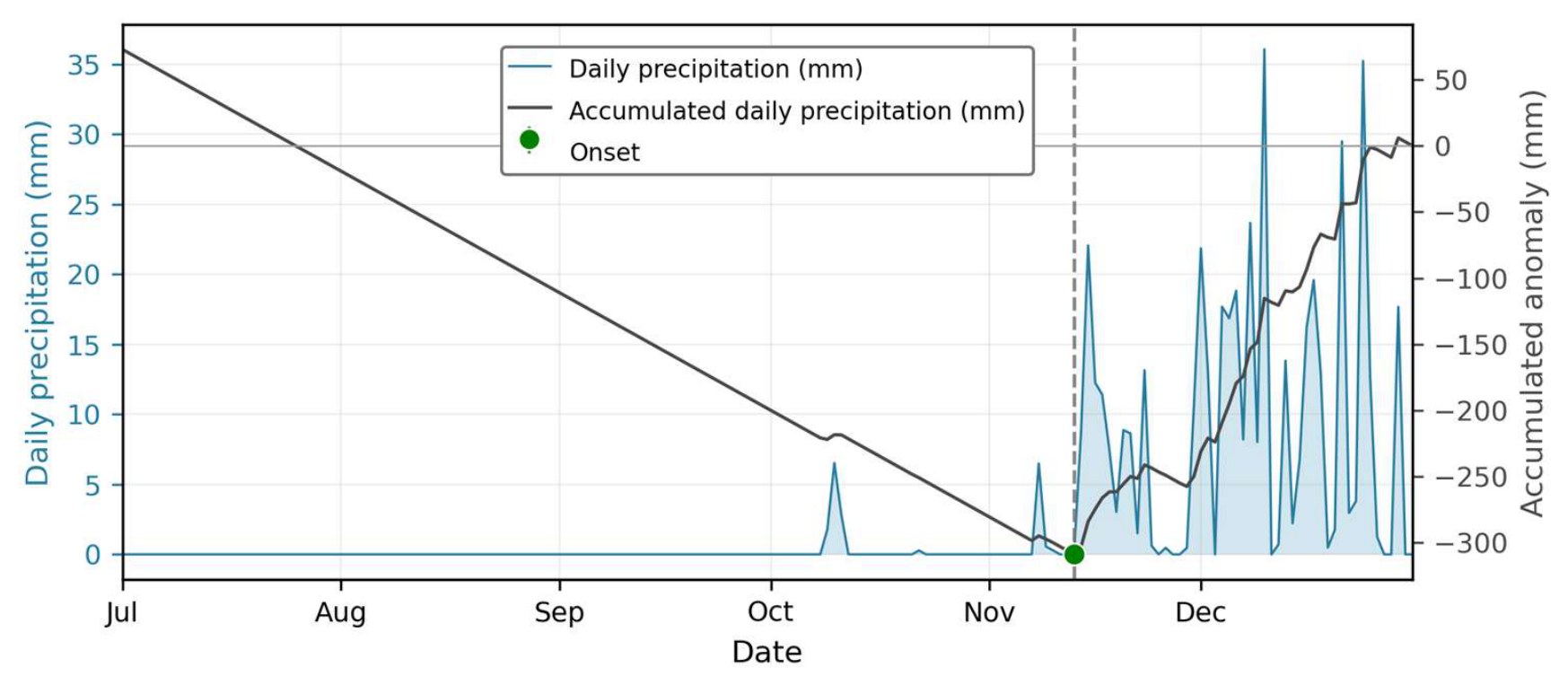
Figure 2.
Example of a dynamical seasonal forecast of the onset from the ECMWF s5.1 system for a specific date and location. The light grey lines show the accumulated daily anomalies for each ensemble member. Green dots indicate the predicted onset date from each ensemble member, while the dashed line indicates the mean predicted onset date across all members.
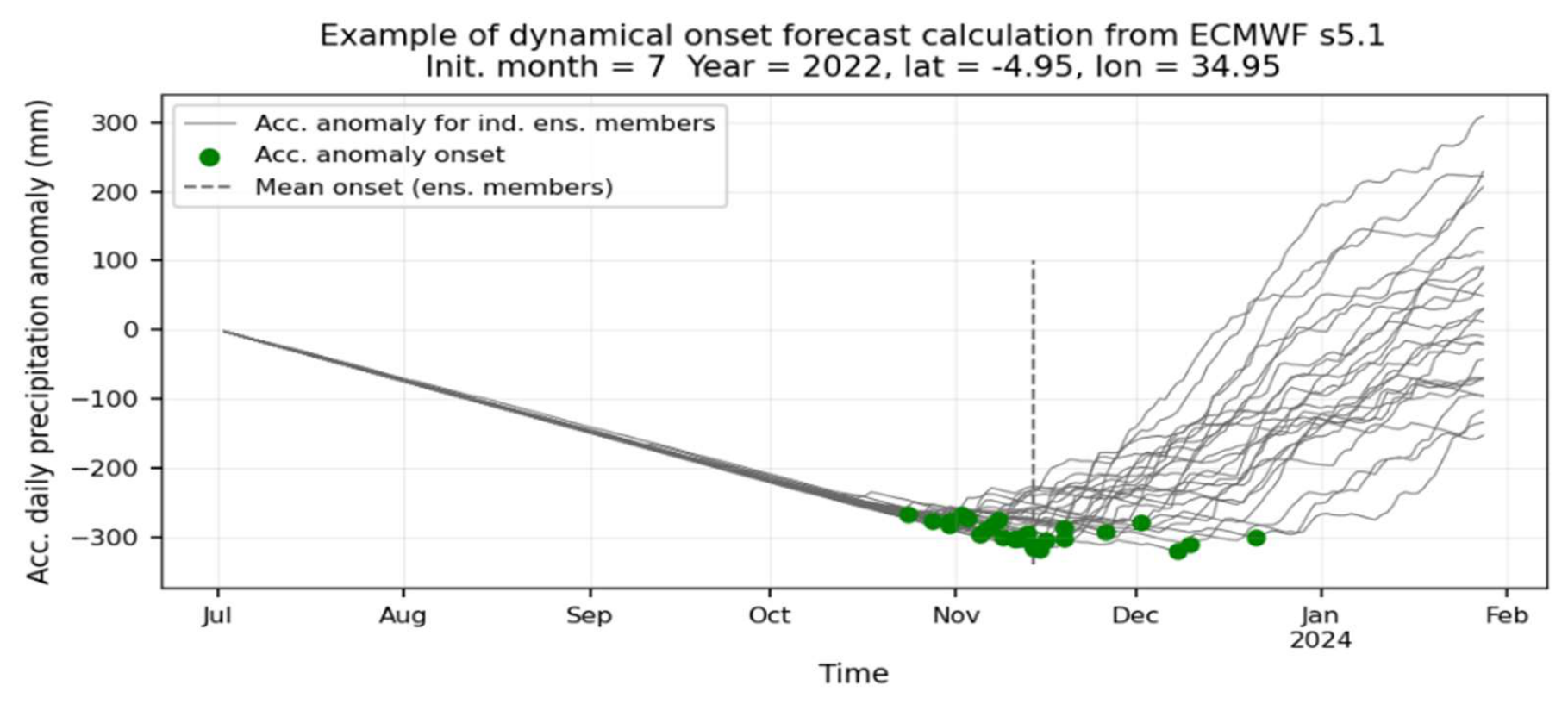
Figure 3.
Tanzania-average Continuous Ranked Probability Skill Score (CRPSS), relative to a leave-one-year-out climatological reference, for Bayesian Ridge, multilayer perceptron (MLP), and Random Forest (RF) at the June–September forecast initialisations. All methods were evaluated using the same reduced predictor set and identical leave-one-year-out hindcast folds.
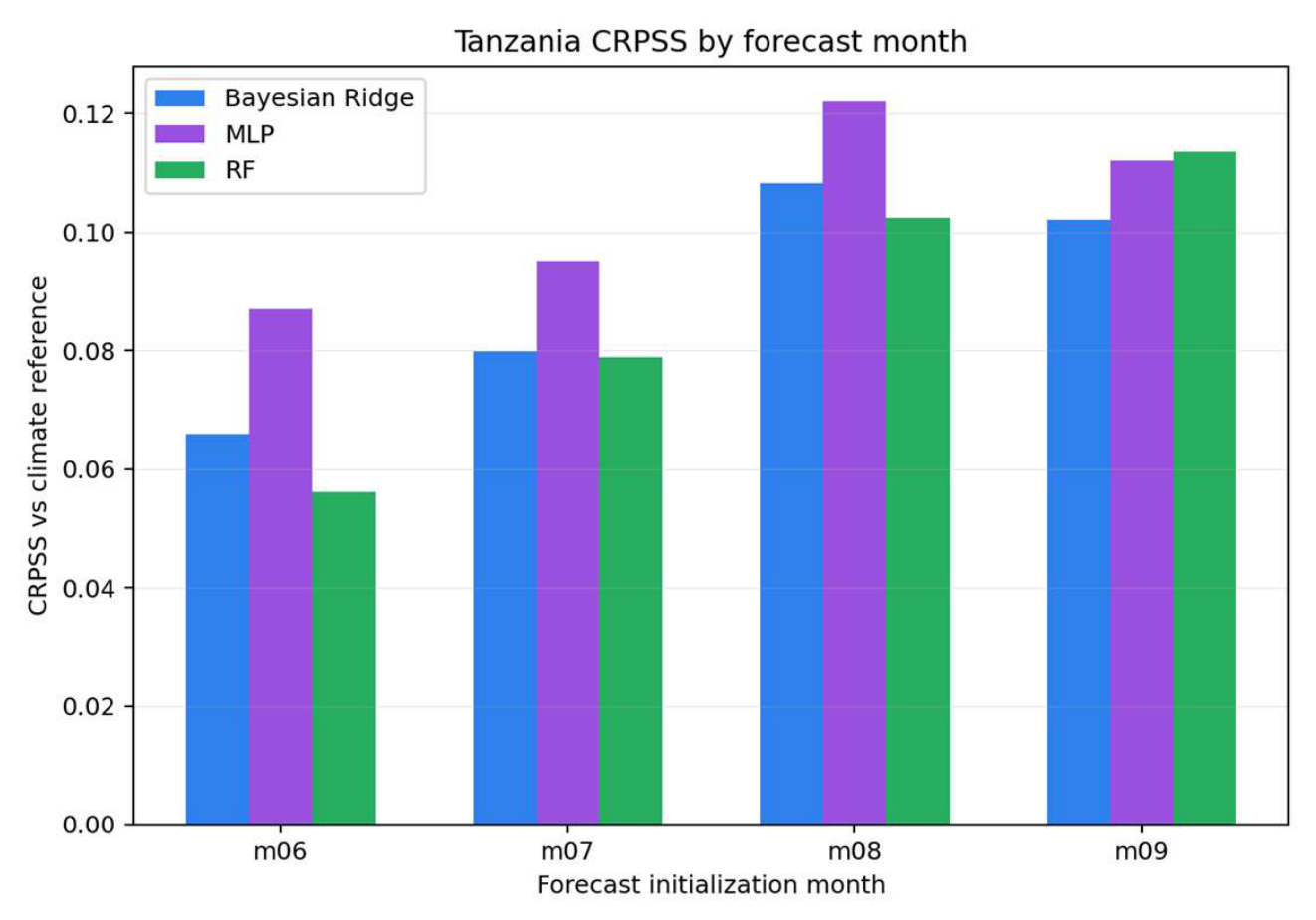
Figure 4.
Average RMSE difference (RF—ECMWF) in days for of OND onset predictions initialised in July. Reddish colours illustrate areas where ECMWF performs better, and blueish colours are areas where our RF model performs better.
Figure 4.
Average RMSE difference (RF—ECMWF) in days for of OND onset predictions initialised in July. Reddish colours illustrate areas where ECMWF performs better, and blueish colours are areas where our RF model performs better.
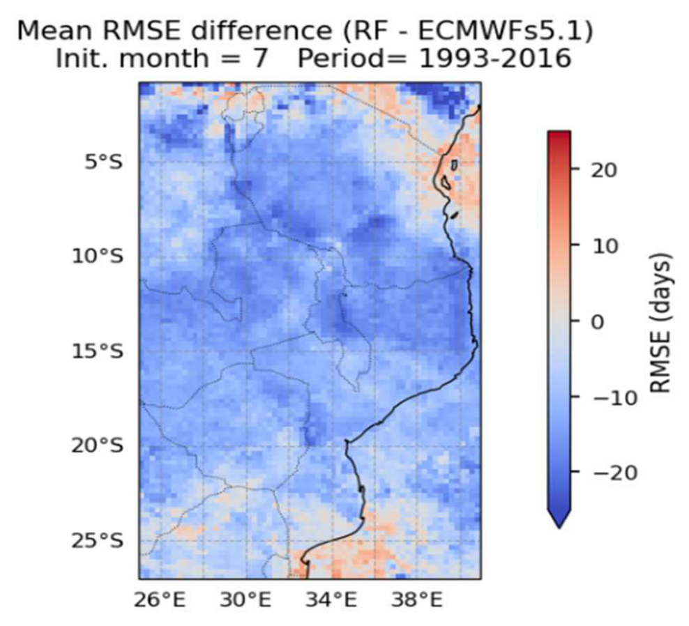
Figure 5.
Mean CRPSS improvement for our RF model compared to the ECMWF s5.1 for July initialisation.
Figure 5.
Mean CRPSS improvement for our RF model compared to the ECMWF s5.1 for July initialisation.
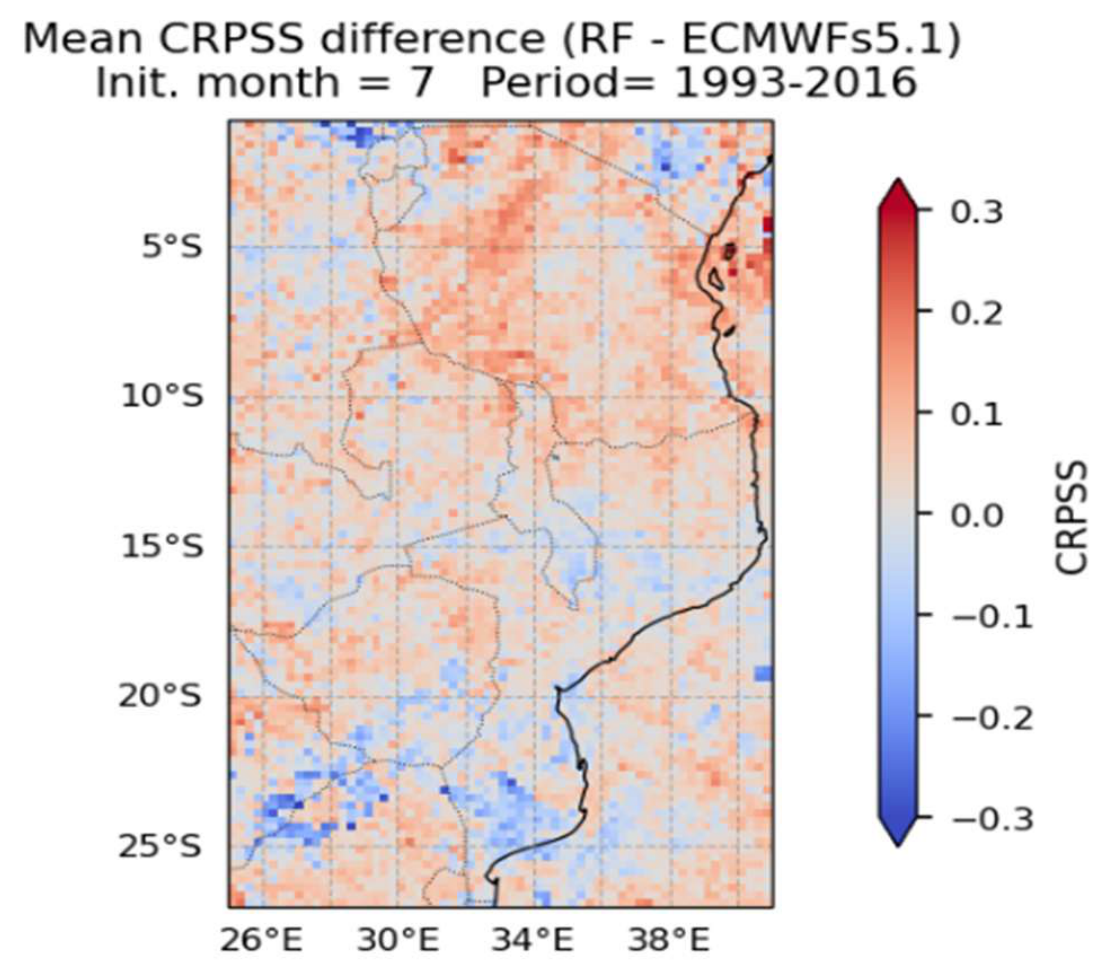
Figure 6.
MSWEP-based RF forecast anomalies of OND onset in days, initialised in July 2023 (left) and July 2024 (right). Orange indicate a later onset, white near normal and bluish an earlier onset, with respect to the reference period 1993-2016.
Figure 6.
MSWEP-based RF forecast anomalies of OND onset in days, initialised in July 2023 (left) and July 2024 (right). Orange indicate a later onset, white near normal and bluish an earlier onset, with respect to the reference period 1993-2016.
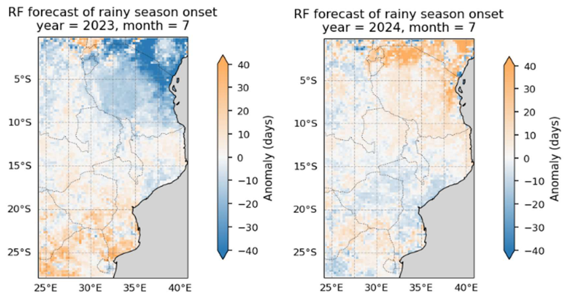
Figure 7.
Calculated onset anomalies from the MSWEP dataset for 2023 OND (left) and 2024 OND (middle). Orange indicates a late onset, white near normal and bluish an earlier onset, with respect to the reference period 1993-2016. The mean onset day of the year with respect to the same reference period is also shown (right) with reddish colours representing later days in the year and bluish earlier.
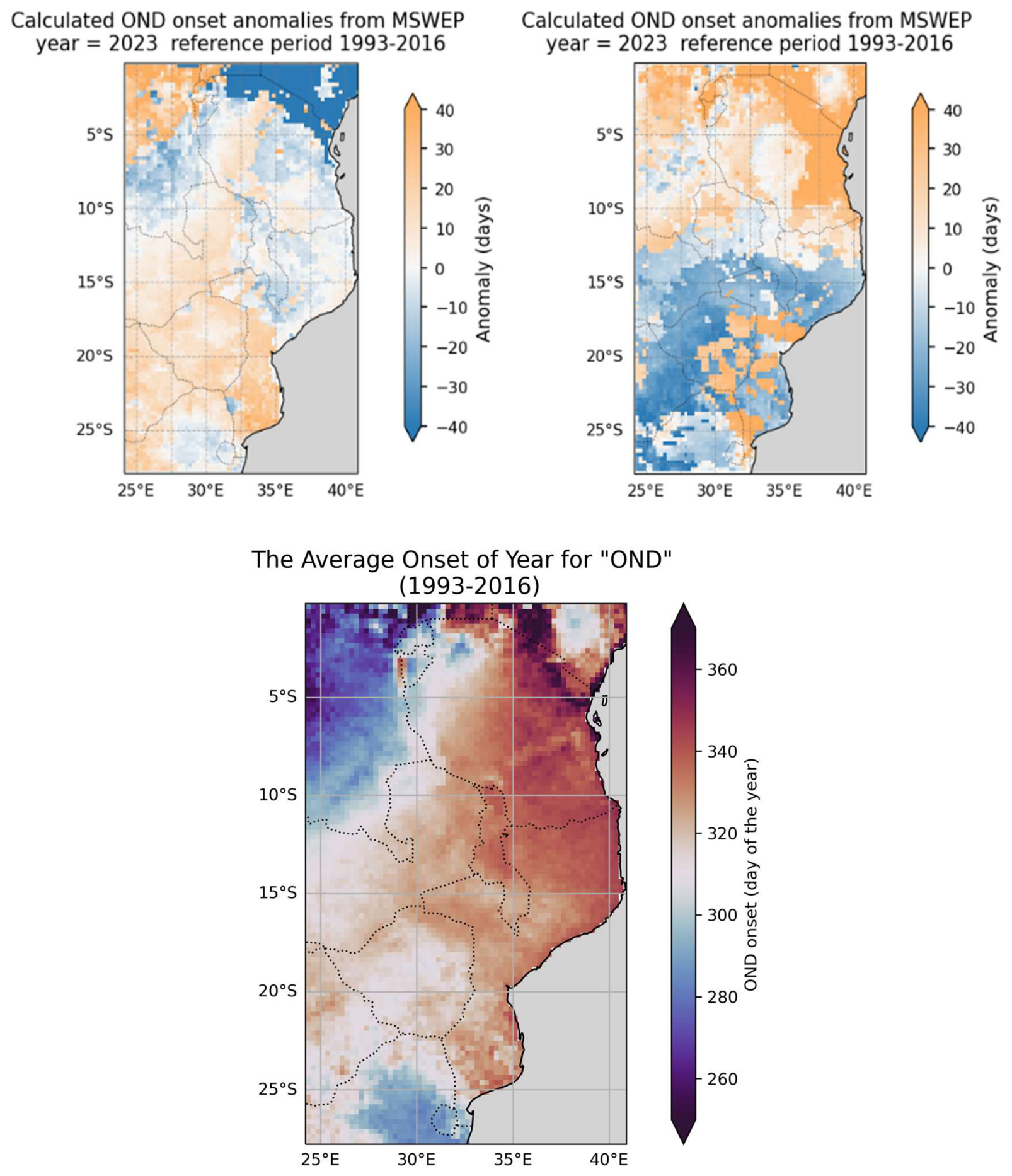
Figure 8.
Predictor importance for our RF forecasts initialised in June (top) and September (bottom). Bars indicate the mean contribution of each predictor across the spatial domain over the years 1993-2016, with variables grouped by category and colour-coded accordingly: direct seasonal forecasts (blue), ENSO forecasts (red), IOD forecasts (green), precipitation observations (purple), ENSO observations (brown), and IOD observations (teal). In predictor labels, fc denotes a forecast variable; the numerical suffix indicates forecast lead time in months for forecast variables and the lag in months for observed variables.
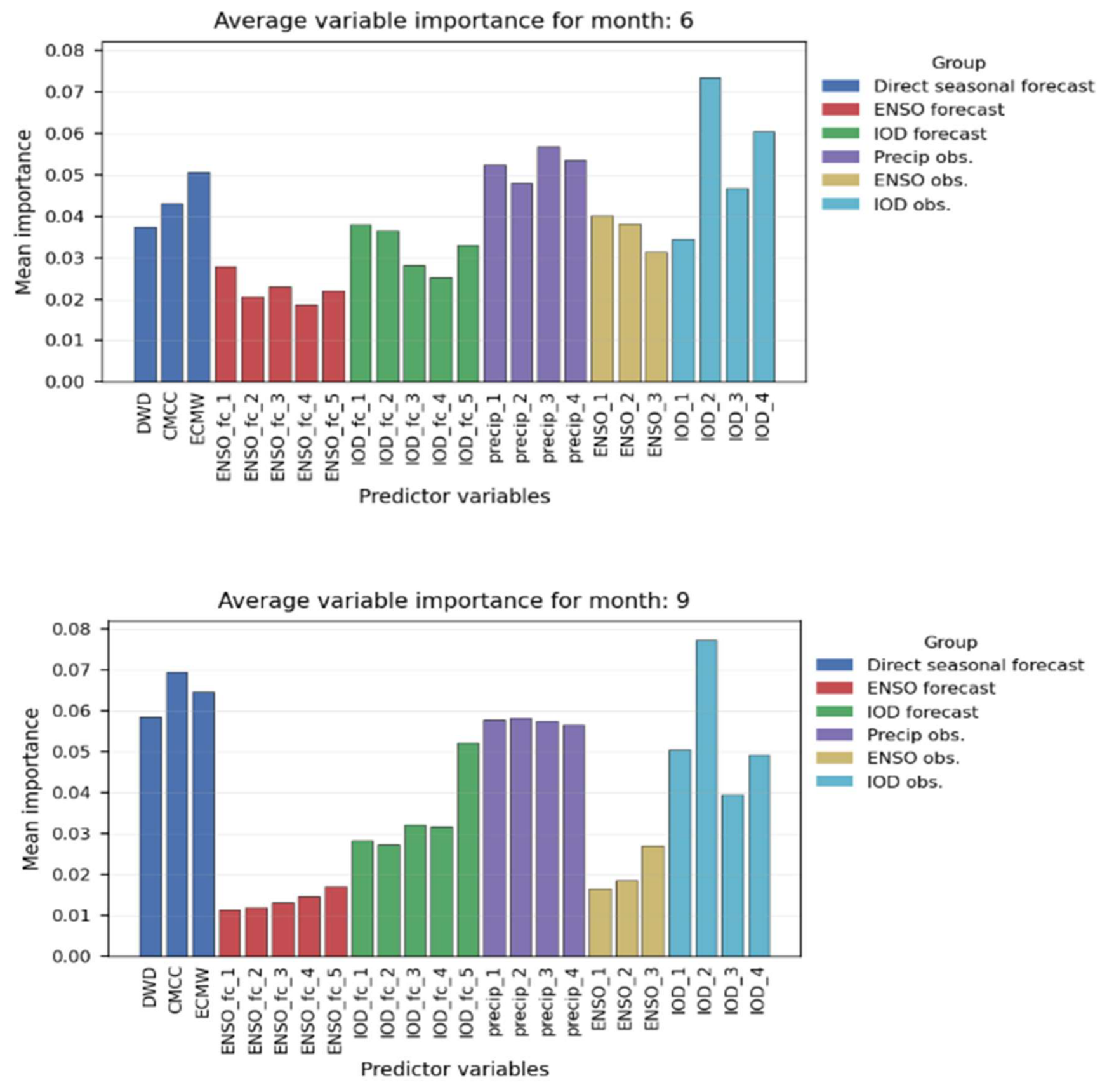
Figure 9.
Onset forecast delivery through a tailored version of the Teal tool developed under the FOCUS-Africa project, which is running operationally and used by TMA. The example shown is the onset prediction for August 2024, with aggregated onset dates across different regions in Southeast Africa.
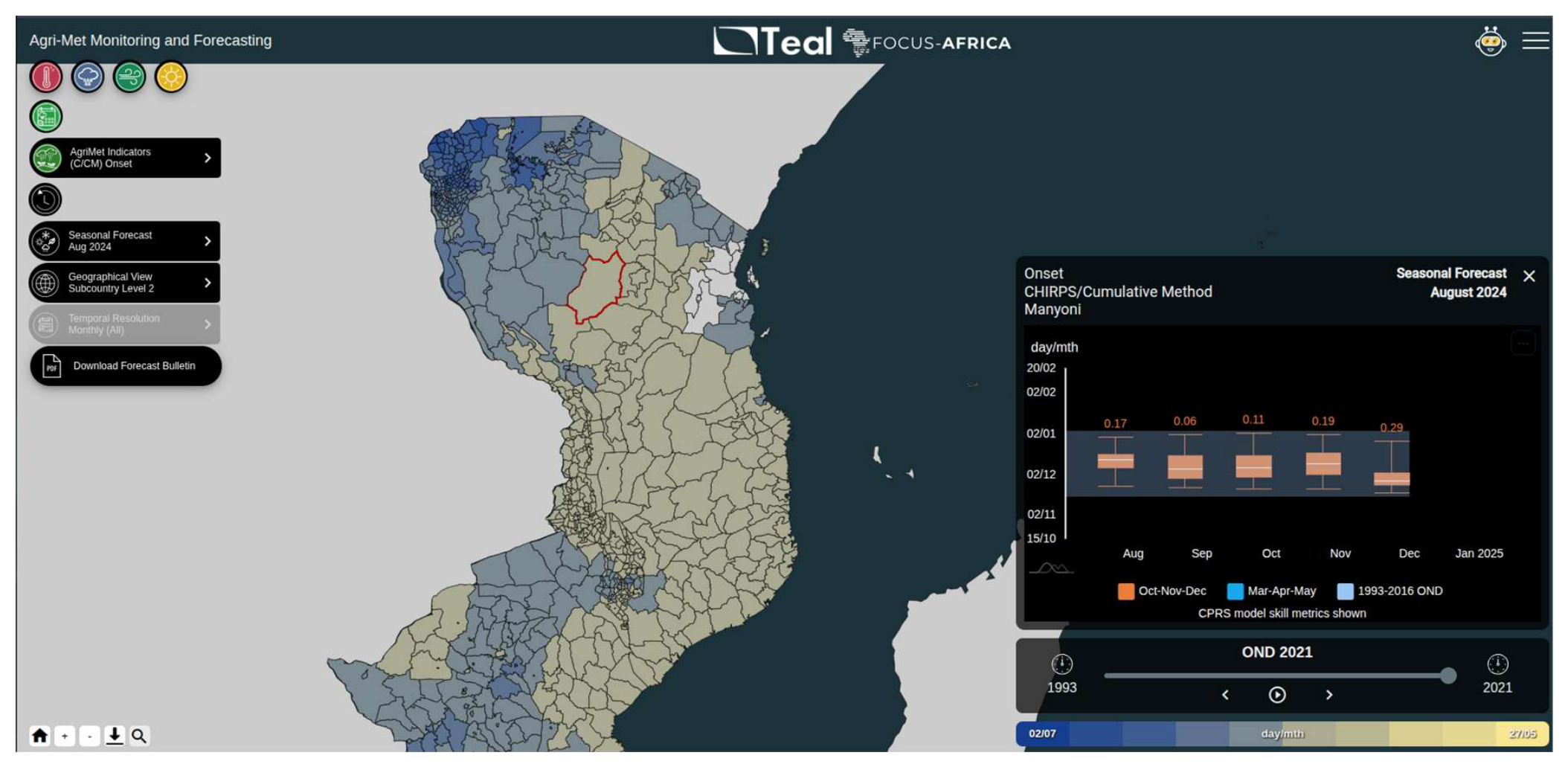

Table 1.
Predictors used in our RF model.
| Predictor (Observations) | Lag (months) | No. of predictors | Source |
|---|---|---|---|
| ENSO 3.4 | 1-3 | 3 | NOAA |
| IOD | 1-4 | 4 | NOAA |
| Observed monthly precipitation1 | 1-3 | 3 | GloH2O, IRI |
| Predictor (Forecasts) | Lead (months) | Source | |
| Onset forecast from ECMWF s5.1 | 1-5 | 1 | CDS |
| Onset forecast from DWD s2.1 | 1-5 | 1 | CDS |
| Onset forecast from CMCC s3.5 | 1-5 | 1 | CDS |
| ENSO 3.4 forecast from multi model | 1-5 | 5 | CDS |
| IOD forecast from multi model. | 1-5 | 5 | CDS |
1 From either MSWEP or CHIRPS as two separate systems are used.
Table 2.
Difference in RMSE (days) between our RF model and ECMWF forecasts across countries for initialisation months June to September. Positive values indicate higher error for our RF model, while negative values represent improvements relative to ECMWF.
Table 2.
Difference in RMSE (days) between our RF model and ECMWF forecasts across countries for initialisation months June to September. Positive values indicate higher error for our RF model, while negative values represent improvements relative to ECMWF.
| Month | Burundi | Malawi | Mozambique | Rwanda | Tanzania | Zimbabwe |
|---|---|---|---|---|---|---|
| Jun | 2 | -5 | -2 | 3 | 3 | 1 |
| Jul | -3 | -6 | -7 | 2 | -5 | -6 |
| Aug | -2 | -7 | -6 | 0 | -7 | -5 |
| Sep | -9 | -15 | -13 | 3 | -12 | -10 |
Table 3.
CRPSS improvement (our RF model compared to the ECMWF s5.1) by country and initialisation month. CRPSS for ECMWF s5.1 compared to climatology is shown in parentheses after the improvements.
Table 3.
CRPSS improvement (our RF model compared to the ECMWF s5.1) by country and initialisation month. CRPSS for ECMWF s5.1 compared to climatology is shown in parentheses after the improvements.
| Month | Burundi | Malawi | Mozambique | Rwanda | Tanzania | Zimbabwe |
|---|---|---|---|---|---|---|
| Jun | +0.03(-0.08) | +0.02(-0.02) | +0.04(-0.04) | +0.02(-0.1) | +0.09(-0.05) | +0.04(-0.01) |
| Jul | +0.05(-0.06) | +0.04(-0.03) | +0.02(-0.02) | +0.03(-0.09) | +0.10(-0.02) | +0.05(-0.01) |
| Aug | +0.06(-0.05) | +0.01(-0.02) | +0.02(-0.01) | -0.08(-0.1) | +0.15(-0.04) | +0.06(-0.01) |
| Sep | +0.09(-0.01) | +0.02(-0.04) | +0.05(-0.02) | +0.02(-0.05) | +0.14(-0.02) | +0.04(-0.00) |
Disclaimer/Publisher’s Note: The statements, opinions and data contained in all publications are solely those of the individual author(s) and contributor(s) and not of MDPI and/or the editor(s). MDPI and/or the editor(s) disclaim responsibility for any injury to people or property resulting from any ideas, methods, instructions or products referred to in the content. |
© 2026 by the authors. Licensee MDPI, Basel, Switzerland. This article is an open access article distributed under the terms and conditions of the Creative Commons Attribution (CC BY) license.
Copyright: This open access article is published under a Creative Commons CC BY 4.0 license, which permit the free download, distribution, and reuse, provided that the author and preprint are cited in any reuse.