
Submitted:
29 September 2026
Posted:
30 September 2026
You are already at the latest version
Abstract
Uneaten feed increases production costs and contributes to water-quality deterioration in shrimp farming, while manual feed-tray inspection is labor-intensive and difficult to sustain for continuous monitoring. Effective feeding assessment requires both residual-feed quantity and spatial distribution, because similar pellet counts can conceal different accumulation patterns. However, existing detection methods struggle with tiny, overlapping pellets and do not directly produce continuous density maps, whereas standalone density estimators are susceptible to underwater background interference. To address these limitations, this study proposes YOLO-SPD-LSK-DGD, an end-to-end network that jointly predicts pellet bounding boxes and spatial density maps through a shared backbone. Detail-preserving downsampling and adaptive contextual feature selection strengthen tiny-pellet representations while suppressing interference from tray grids and water-surface reflections. A hybrid bounding-box regression loss combines overlap-based geometric constraints with distribution-based similarity to improve localization stability for densely clustered pellets. Furthermore, density supervision is automatically generated from existing bounding-box centers using bounded Gaussian bandwidths determined by local nearest-neighbor distances. This strategy accommodates variations in pellet spacing without requiring additional manual point annotations. Experiments on a field-collected shrimp feed-tray dataset achieved an mAP50 of 0.9231 for detection and an R² of 0.9004 for counts obtained by integrating predicted density maps. Evaluation across different accumulation conditions and analysis of failure cases further characterize the model’s performance and limitations under challenging field conditions. These results support the feasibility of jointly locating residual feed and describing its spatial accumulation, providing complementary information for quantitative monitoring and supporting more informed feeding decisions in shrimp aquaculture.
Keywords:
shrimp aquaculture
; uneaten feed
; spatial density maps
; bounding-box regression
; end-to-end network
1. Introduction
Feed can account for approximately half or more of shrimp production costs, making feeding management important for both profitability and environmental sustainability. Uneaten feed increases organic loading and oxygen demand. Its decomposition releases ammonia nitrogen, while incomplete nitrification can contribute to nitrite accumulation, worsening water quality and increasing animal-health risks. Manual feed-tray inspection remains labor-intensive and provides intermittent, subjective observations. IoT-based monitoring and wireless sensor networks have been developed to monitor aquaculture environments [1,2], while automated and smartphone-controlled feeding systems support feeding operations [3,4]. For residual-feed assessment, however, total pellet counts alone cannot distinguish dispersed pellets from localized accumulations. This distinction could help identify uneven feed deposition or consumption. Spatial distribution therefore provides complementary information for feeding assessment, motivating the joint detection of pellets and estimation of their spatial density.
Existing approaches follow two main routes. Detection-based methods, particularly improved YOLO models, identify individual pellets but remain vulnerable to feature loss, overlap, and underwater interference [5,32]. Tiny bounding boxes are sensitive to small coordinate shifts, which can destabilize regression based on geometric overlap. Although detection boxes preserve locations, count-only outputs discard spatial arrangement and do not directly describe continuous accumulation. The second route includes density-map regression, represented by MCNN, and point-based counting, represented by P2PNet [33,34]. These methods offer alternative abundance representations but require adaptation to reflective, textured underwater backgrounds. Density estimation has already been applied to shrimp residual feed [35], yet standalone counting does not inherently provide bounding boxes. Detection followed by kernel density estimation also inherits detection errors and adds a processing stage whose latency must be considered for field deployment.
Three research gaps remain. First, integrated networks jointly producing bounding boxes and continuous density maps are insufficiently investigated for tiny, highly aggregated shrimp-feed residues. Second, preserving weak pellet features and stabilizing localization under grid textures, reflections, and overlap remain interconnected challenges. Third, fixed-bandwidth supervision cannot accommodate substantial variations in pellet spacing. Although geometry-adaptive kernels already exist, their use with bounding-box-derived supervision requires task-specific integration and evaluation.
To address these gaps, this study develops YOLO-SPD-LSK-DGD. The main contributions are as follows. (1) To reduce feature loss and background interference, an SPD-Conv and C2f-LSK backbone preserves fine spatial information and adaptively selects contextual features. A hybrid Focaler-CIoU and normalized Wasserstein distance loss combines overlap-related constraints with distribution-based similarity to improve regression for tiny, crowded pellets. (2) A shared-backbone detection–density framework jointly predicts individual locations and continuous accumulation patterns. Bounded Gaussian bandwidths are determined by local nearest-neighbor distances, and density supervision is generated automatically from bounding-box centers, avoiding additional manual point labeling. The contribution is the adaptation and integration of this supervision strategy rather than nearest-neighbor kernel estimation itself. (3)A field-collected shrimp feed-tray dataset supports comparative experiments, ablation studies, detection and density evaluation, and analyses across different stacking conditions. Failure cases further identify limitations associated with reflections, background interference, and severe overlap, assessing the feasibility of quantitative residual-feed monitoring.
2. Related Work
Recent aquaculture studies have adapted visual detectors to underwater feed pellets. Hu et al. improved YOLOv4 for tiny-pellet detection [5], Xu et al. incorporated attention and a small-object detection layer into YOLOv5 [31], and Hu et al. combined YOLO and Mask R-CNN [32] for residual-feed recognition in swimming-crab culture. These developments build on advances in efficient YOLO architectures [11,27,28] and address limited visual information and background interference identified in small-object detection research [9,10]. Feature fusion and contextual modeling have also been explored through improved SSD and dedicated small-target networks [12,13]. SPD-Conv and its detection applications preserve fine-scale information during downsampling [14,15], while selective large-kernel networks adapt spatial context [16,17]. Localization research further includes IoU-based optimization [18], normalized Wasserstein distance for tiny objects [19], and Focaler-IoU for adjusting regression focus [20]. Nevertheless, these techniques require validation under shrimp-tray reflections, mesh textures, and pellet overlap. Detection-focused feed-monitoring methods primarily produce discrete instances rather than jointly learned continuous density maps, motivating integrated localization and accumulation assessment.
Density regression represents object abundance through continuous maps, as reviewed in crowd-counting studies [6,7]. MCNN combines multiscale features with geometry-adaptive Gaussian supervision [33], whereas W-Net explores encoder–decoder density estimation [26]. P2PNet directly predicts object centers rather than continuous density maps [34] . Joint counting, density estimation, and localization have already been investigated in crowd analysis [8,24], while plant detection and leaf counting illustrate related integration in agricultural phenotyping [23]. These studies support exploiting related tasks through shared representations [22]; neither joint prediction nor adaptive Gaussian supervision alone constitutes a new contribution. In aquaculture, Zhang et al. estimated shrimp residual-bait density [35] using hybrid dilated convolution and multiscale attention. However, transferring these approaches to shrimp trays requires distinguishing pellets from grid intersections and reflections while accommodating variable spacing. Fixed Gaussian bandwidths cannot follow local spacing changes, whereas unconstrained adaptive bandwidths may become inappropriate in extreme distributions. This motivates bounded adaptive supervision derived from existing bounding-box centers within a shared detection–density framework, avoiding additional manual point annotations.
Aquaculture monitoring includes IoT-based environmental sensing [1,2] and automated or remotely controlled feeding [3,4]. Underwater vision research has also investigated fish classification [21] and behavior recognition [29,30], extending monitoring beyond water-quality measurements. More recent applications include camera-based prawn assessment during feed-tray inspection [36], acoustic assessment of fish feeding intensity [37], and outdoor feeding assessment through fish detection and counting [38] . These approaches provide complementary operational information but do not directly characterize residual-feed accumulation. Studies of feed and fecal-solid settling [39] and aquaculture digital twins [40] further broaden the context for linking observations with production processes. Nevertheless, environmental conditions, animal behavior, and residual-feed distribution describe different aspects of feeding management. Reliable joint estimation of pellet locations and continuous spatial density under field interference remains the specific problem addressed here. Translating these outputs into feed-mass estimates or validated closed-loop feeding decisions requires further investigation.
3. Materials and Methods
This study develops an end-to-end perception network with a shared backbone and dual branches based on the YOLOv8s architecture, as illustrated in Figure 1.
Shallow feature representations are extracted from the input images through the SPD-Conv backbone with lossless downsampling. C2f-LSK attention blocks are incorporated at the backbone output and into the P3, P4, and P5 detection heads. The resulting feature maps are then fed into two parallel branches. In the detection branch, residual feed pellets are localized and classified using a hybrid loss combining Focaler-CIoU and NWD. The density estimation branch directly reuses high-level features from the P5 layer and restores spatial resolution through transposed and standard convolutions to generate global and local density heatmaps. The entire network is trained end-to-end using a unified weighted loss function.
3.1. An Improved YOLOv8s Detection Backbone Network
3.1.1. Full-Trunk SPD Downsampling Architecture
To reduce the loss of fine-grained texture information caused by conventional strided convolution and pooling in shallow layers, Spatial-to-Depth Convolution (SPD-Conv) is used to replace all stride-2 downsampling convolutions in the backbone [14].
Figure 2.
Schematic illustration of lossless downsampling using SPD-Conv.
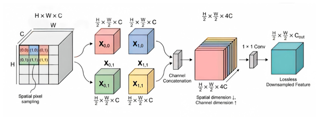
For an input feature map of size H×W×C, the transformation performed by SPD-Conv can be described as follows.
First, the feature map is spatially partitioned using a slicing factor of 2, producing four sub-feature maps:
Each sub-feature map has a size of  . The four sub-feature maps are then concatenated along the channel dimension to form a reconstructed feature map of size
  .
.
. The four sub-feature maps are then concatenated along the channel dimension to form a reconstructed feature map of size .Finally, a 1×1 convolution is applied to map the 4C channels to the target number of output channels  . This operation reduces the spatial resolution while preserving the original pixel information.
. This operation reduces the spatial resolution while preserving the original pixel information.3.1.2. C2f-LSK Attention Bottleneck Unit
The LSK (Large Selective Kernel) attention mechanism is integrated into the C2f module of YOLOv8s to construct the C2f-LSK unit, which is deployed in the deeper backbone layers and the P3, P4, and P5 feature pyramid levels [16,17].
Figure 3.
Structural diagram of the LSK selective large-core attention module.
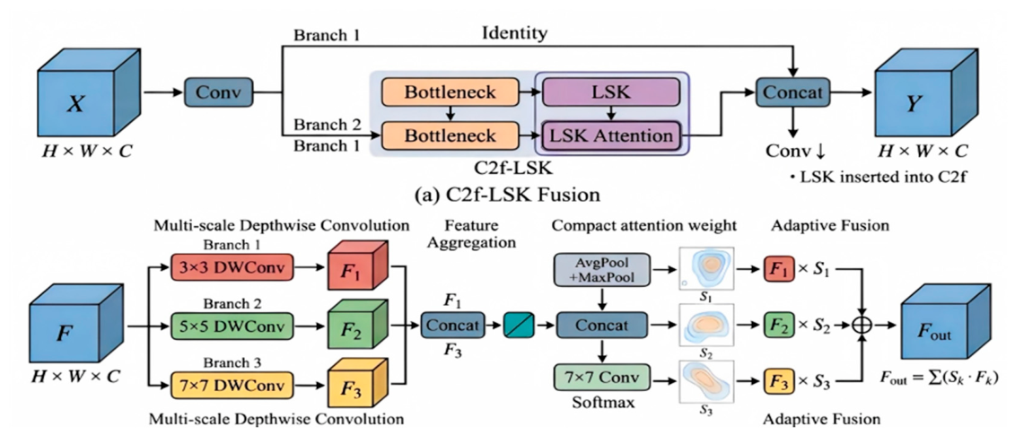
Let the input feature map be X ∈ ℝC×H×W. The LSK module employs multiple convolutional branches with different kernel sizes k = {3,5,7}:
Perform global average pooling on each branch to obtain the channel representation:
After dimension reduction and upsampling using a shared single-layer MLP, multi-branch adaptive weights are generated via Softmax:
Weighted fusion of multiscale features on a per-channel basis based on weights:
Here, ⊙ denotes element-wise multiplication. The adaptive weights enhance feature responses associated with small residual feed pellets while suppressing interference from water-surface reflections and feed-tray grid patterns. The FLSK is then fed into the residual branch of the C2f module to promote cross-channel feature interaction, thereby progressively enhancing residual-feed features from shallow fine-grained details to deeper semantic representations.
3.1.3. Focaler-CIoU and NWD Hybrid Boundary Loss
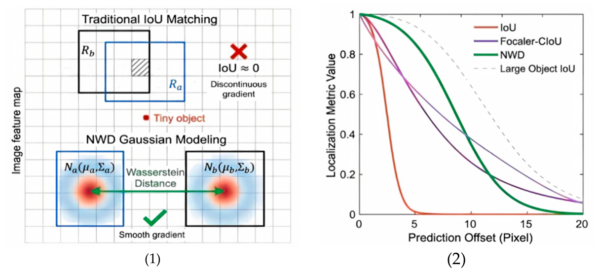
Construction of a Weighted Joint Loss Combining Focaler-CIoU [20] and NWD [19]: Focaler-CIoU applies interval-based weighting to emphasize difficult samples in densely overlapping regions, whereas NWD models bounding boxes as two-dimensional Gaussian distributions to alleviate weak or vanishing gradients for extremely small targets. The weighted combination of the two losses improves the stability and accuracy of bounding-box regression for slender and densely clustered residual feed pellets.
Figure 4.
(1) Schematic Diagram of the NWD and Focaler-CIoU Combined Loss Function. (2) NWD vs. Focaler-CIoU Curve.
Figure 4.
(1) Schematic Diagram of the NWD and Focaler-CIoU Combined Loss Function. (2) NWD vs. Focaler-CIoU Curve.
(1)NWD Loss Function
NWD models the residual bait bounding box 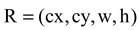 as a two-dimensional Gaussian distribution
  , where:
as a two-dimensional Gaussian distribution , where:For a predicted distribution a and a true distribution b, the second-order Wasserstein distance between the two can be calculated as follows:
To convert this distance into a metric that can be directly combined with the classification loss, it is constrained to the interval [0,1] via an exponential normalization mapping:
Here, C is a constant determined by the characteristics of the dataset. The NWD loss is expressed as follows. Since NWD measures the distributional distance between bounding boxes rather than relying on their geometric overlap, it can provide smooth and continuous gradients even when two boxes do not overlap, thereby improving the stability of localization for small residual feed pellets.
(2)Focaler-IoU Loss Function
Feed-tray images collected from high-level tanks exhibit a pronounced imbalance between easy and difficult samples. Empty grid cells and other background regions are relatively easy to distinguish, whereas densely adhered pellets and particles located near shadowed edges are considerably more difficult to localize.
Focaler-IoU reconstructs IoU through linear interval mapping, focusing on hard-to-train samples such as wet, overlapping, or stuck-together leftover feed:
By combining the center point of CIoU with the aspect ratio penalty term RCloU, the final Focaler-CIoU loss is expressed as:
(3)Hybrid Loss Fusion Strategy
During the training phase, the two types of loss are combined using equal weighting to produce the total boundary loss:
Focaler-CIoU constrains the center-point offset and aspect ratio of residual feed pellets, whereas NWD compensates for insufficient gradient information in samples with extremely low IoU. Together, the two losses improve the localization accuracy of densely clustered and elongated residual feed pellets.
3.2. Dynamic Gaussian Density Estimation Branch
Relying solely on detection boxes provides only the total number of residual feed pellets and cannot adequately characterize localized accumulation, which may have a greater impact on water quality. To address this limitation, this study introduces a dynamic Gaussian density regression branch that shares the backbone with the detection branch. By integrating dual-format annotations, adaptive Gaussian ground-truth generation, and a density prediction head, the proposed network simultaneously outputs residual-feed locations and spatial density heatmaps in an end-to-end manner.
3.2.1. Specifications for Dual Annotation of Dataset Center Points
Conventional YOLO datasets annotate residual feed pellets only with bounding boxes(cx,cy,w,h), which cannot be directly used to construct density heatmaps. To address this limitation, this study introduces a dual-annotation mechanism that combines bounding boxes and geometric centers. The center coordinates pi = (xi,yi) of each residual feed pellet are automatically derived from its bounding box to generate ground-truth density maps. This design ensures that the detection and density regression branches use annotations from the same source while avoiding the additional cost of secondary labeling.
3.2.2. Adaptive Dynamic Gaussian True-Value Heatmap Generation
Conventional fixed Gaussian kernels are difficult to adapt to large variations in residual-feed density. If the kernel size is too small, density responses in crowded regions may become fragmented; if it is too large, the boundaries between neighboring particles in sparse regions may become blurred [33]. To address this limitation, this study proposes a dynamic Gaussian generation method that adaptively adjusts the kernel bandwidth according to nearest-neighbor distances:
(1) Calculation of the Local Average Neighbor Distance
For each residual-feed center point in the image, the k nearest neighboring particle centers are identified. Their two-dimensional Euclidean distances are then calculated and averaged to characterize the local particle density. The calculation is given as follows:
Here, di represents the average distance to the i-th residual bait in the local neighborhood; || ⋅ ||2 denotes the Euclidean distance operation in two-dimensional coordinates; k is the number of neighbors selected (in the experiments in this paper, k=4); and j is the index of the current neighboring particle. When residual baits are densely stacked, the spacing between surrounding particles is small, and the di value is low; when the distribution is sparse, the spacing between particles is large, and the di value is correspondingly higher.
(2) Calculation of Adaptive Gaussian Bandwidth Constraints
The initial Gaussian bandwidth is linearly mapped from the mean nearest-neighbor distance,di. Upper and lower bounds are then imposed as clipping constraints to prevent extreme values from producing unstable or overly diffuse density responses. The calculation is given as follows:
Here, σi denotes the Gaussian bandwidth (standard deviation), and α is a scaling factor set to 1.2 in this study. The clipping function constrains the bandwidth to [σmin,σmax]. The lower bound prevents excessively narrow kernels in densely clustered regions, while the upper bound limits excessive spatial spreading in sparse regions. Within these bounds, smaller nearest-neighbor distances produce narrower kernels, whereas larger distances produce broader kernels. This strategy adapts the spatial extent of density responses to local pellet spacing while limiting extreme bandwidth values.
(3) Generation of the Global True-Value Density Map by Superposition
For the center of each residual feed pellet in the image, a two-dimensional Gaussian distribution is constructed using the adaptively determined bandwidth σi [26]. The Gaussian responses of all pellets are then superimposed pixel by pixel to generate the complete ground-truth density mapDgt(x,y), which is calculated as follows:
Here,(x,y) denotes the coordinates of a pixel in the density map; N is the total number of residual feed pellets in a single feed-tray image; (xi,yi) denotes the center coordinates of the i-th pellet; and σi is the adaptively estimated Gaussian bandwidth for the i-th pellet. The pixel values in the density map represent the spatial distribution of residual feed, with higher values indicating greater local accumulation.
3.2.3. Density-Regressive Head Network Architecture
The density regression branch takes the high-level feature map from the P5 layer of the backbone as input. The feature map is first restored to the spatial resolution of the original image through a transposed convolution with a stride of 8[26,32]. It is then passed through two successive 3×3convolutions, each followed by batch normalization (BN) and ReLU activation, to reduce the channel dimension and extract density-related features. Finally, a 1×1 convolution followed by a Sigmoid activation normalizes the pixel values to the range [0, 1],, producing the predicted density map, where H and W denote its height and width, respectively.
3.3. Detection-Density Joint Weighted Loss Function
This paper employs a dual-task joint learning [22] architecture that simultaneously optimizes the detection branch, the density branch, and the shared backbone parameters via a weighted total loss function:
3.3.1. Detecting Branch Loss det
The detection branch loss is divided into two major modules: target classification loss and bounding box regression combined loss. The complete expression is:
In particular, the classification loss cls is used to distinguish the leftover bait from the background; the bounding box loss bboxemploys an equally weighted combination of the Focaler-CIoU loss and the NWD loss.
3.3.2. Density Branch Loss density
Use the MSE to constrain, on a pixel-by-predicted-pixel basis, the deviation in distribution between the predicted density map D and the true density map Dgt:
Here, H and W represent the height and width of the density heatmap, respectively; D(x,y) is the pixel density value predicted by the model, and Dgt(x,y) is the true pixel density value generated by dynamic Gaussian; the mean squared error between the predicted values and the true values for all pixels in the entire heatmap—the smaller the value, the closer the model’s predicted spatial distribution of leftover bait is to the actual distribution, and the lower the counting and regional density errors.
4. Experimental Results and Discussion
4.1. Datasets and Experimental Environment
A total of 621 original images were collected from high-density shrimp farming ponds under different lighting conditions and at different sampling times. Before image slicing or augmentation, the original images were divided into training, validation, and test sets at an approximate ratio of 7:2:1. Overlapping sliding-window slicing was subsequently performed within each subset to generate 640 × 640 image patches. All patches derived from the same original image were retained in the same subset. Random data augmentation, including geometric transformations, HSV perturbation, blurring, and occlusion, was applied exclusively to the training set. No random augmentation was applied to the validation or test set. This procedure prevented overlapping patches and augmented variants of the same original image from being distributed across different subsets;The experimental hardware consisted of an RTX 4060 laptop graphics card and an i7 processor, running on Windows 11 with PyTorch 2.6.0. A fixed random seed was used, and training was conducted at full FP32 precision. Evaluation metrics included mAP50, mAP50–95, precision, recall, APsmall for small objects, MAE for counting, and FPS for inference.
4.2. Evaluation Indicator System
4.2.1. Object Detection Evaluation Metrics
(1)Precision: The proportion of samples correctly predicted as leftover bait among the samples actually containing leftover bait:
(2)Recall Rate: The proportion of all actual leftover bait that was successfully detected:
In this context, TP refers to a true positive (correct detection of bait residue); FP refers to a false positive (mistaken identification of a grid or water stain as bait residue); and FN refers to a false negative (failure to detect bait residue particles).
(3)AP and mAP: Average Precision (AP) is defined as the area under the Precision–Recall (PR) curve for the residual-feed class. Mean Average Precision (mAP) is obtained by averaging AP across classes. Since only one object class is considered in this study, mAP is numerically equivalent to AP. mAP@0.5 denotes the metric evaluated at an IoU threshold of 0.5, while mAP@0.5:0.95 represents the average over IoU thresholds from 0.5 to 0.95 with a step size of 0.05 [27,28].
(4) APsmall: AP calculated exclusively for small targets with a pixel area smaller than 32×32, suitable for evaluation using 5×5 to 15×15 pixel residual masks.
(5) FPS: The number of images that can be processed per second, indicating the model’s real-time inference speed.
4.2.2. Metrics for Evaluating Density Estimation
By summing the predicted density map globally, we obtain the total number of predicted residuals, , and the total number of true values, Ngt. We use the following four quantification error metrics:
(1) Mean Absolute Error (MAE):
(2)Root Mean Square Error (RMSE)
(3) Mean Relative Error (MRE):
Here, M represents the total number of images in the test set.
(4) Coefficient of determination R2: This measures the degree of linear fit between the predicted values and the true values; the closer it is to 1, the better the fit.
4.3. Comparative Experiment
To verify the comprehensive competitive advantages of the improved model YOLOv8s-SPD-LSK proposed in this paper, we conducted comparative experiments using the same dataset and training parameters against the classic two-stage detector (Faster R-CNN) and mainstream lightweight models in the YOLO series (YOLOv5s, YOLOv9s, YOLOv10s, YOLOv11s, and YOLOv26s). The experimental results are shown in Table 4-1.

Table 4-1.
Experimental Results Comparing Different Detection Models.
| Models | mAP50 | mAP50-95 | Precision | Recall | APsmall | MAE | FPS |
|---|---|---|---|---|---|---|---|
| YOLOv5s | 0.7879 | 0.2561 | 0.7603 | 0.7789 | 0.3563 | 1.01 | 105.6 |
| YOLOv9s | 0.7778 | 0.2602 | 0.7650 | 0.7637 | 0.3315 | 1.33 | 54.7 |
| YOLOv10s | 0.7819 | 0.2692 | 0.7647 | 0.7666 | 0.3506 | 1.88 | 106.1 |
| YOLOv11s | 0.7781 | 0.2593 | 0.7658 | 0.7646 | 0.3351 | 1.28 | 92.8 |
| YOLOv26s | 0.7850 | 0.2662 | 0.7635 | 0.7002 | 0.3495 | 2.32 | 85.0 |
| Faster R-CNN | 0.6938 | 0.2156 | 0.8149 | 0.7589 | 0.2145 | 1.88 | 22.6 |
| YOLOv8s-SPD-LSK | 0.9231 | 0.3668 | 0.9163 | 0.9139 | 0.9193 | 0.81 | 100.8 |
The results in Table 4-3 demonstrate that the proposed modifications improve detection performance. Compared with the baseline YOLOv8s, the complete model achieves an mAP50 of 0.9231, an mAP50–95 of 0.3668, and an APsmall of 0.9193, corresponding to gains of 13.29, 10.16, and 16.11 percentage points, respectively. Precision and recall reach 0.9163 and 0.9139. These improvements support the combined effectiveness of detail-preserving feature extraction, contextual modeling, and modified bounding-box regression for tiny residual-feed detection. However, counting accuracy does not improve consistently: MAE increases from 0.74 to 0.81, and RMSE increases from 1.41 to 1.45. Thus, the complete model provides stronger detection performance while retaining relatively low counting errors, rather than achieving the best results across every metric. This difference also indicates that improvements in detection metrics do not necessarily translate into lower errors in counts derived from detected instances.
4.4. Ablation Experiment
To thoroughly analyze the independent contributions of the preprocessing strategy, various network architecture modules, and loss functions to detection performance, we conducted multidimensional ablation experiments.
4.4.1. Data Preprocessing and Feature Engineering Ablation Experiments
Using the original YOLOv8s as the baseline [28], we evaluate the effectiveness of Overlapping Sliding Window Slicing (OSWS) and targeted data augmentation. If the original image is directly resized for training, tiny residual target pixels are severely compressed, resulting in an extremely low APsmall; after introducing OSWS slicing, the fine details of tiny targets are fully preserved, and detection performance is significantly improved; with the addition of geometric, illumination, and occlusion enhancements, the model’s robustness against glare and noise is further enhanced. The experimental results are shown in Table 4-2.
Table 4-2.
Experimental Results for Different Data Preprocessing and Feature Enhancement Methods.
| Preprocessing Operations | mAP50 | mAP50-95 | P | R | MAE | RMSE | APsmall |
|---|---|---|---|---|---|---|---|
| Original image | 0.2896 | 0.0757 | 0.6051 | 0.3990 | 4.44 | 7.46 | 0.0735 |
| Overlapping sliding window slicing | 0.7423 | 0.3635 | 0.8252 | 0.7423 | 1.84 | 4.16 | 0.3767 |
| Slicing + spatial geometric transformation enhancement | 0.8397 | 0.3080 | 0.8832 | 0.8646 | 1.32 | 2.56 | 0.3093 |
| Slicing + geometric transformation + HSV lighting perturbation enhancement | 0.8478 | 0.3106 | 0.8830 | 0.8701 | 1.41 | 2.62 | 0.3109 |
| Slicing + geometric transformation + lighting + blurring and occlusion-full suite of enhancements | 0.8481 | 0.3107 | 0.8823 | 0.8692 | 1.53 | 2.74 | 0.3112 |
To evaluate the effects of multi-resolution overlapping sliding-window slicing (OSWS) and hybrid data augmentation on the detection and counting of tiny residual feed pellets, five sets of ablation experiments were conducted using the same YOLOv8s-SPD-LSK architecture and training hyperparameters. (1) Effect of OSWS slicing: When the original images were directly downsampled for training, the model achieved an mAP50 of 0.2896, a recall of 0.3990, and an APsmall of only 0.0735. The false-negative rate exceeded 60%, resulting in a relatively large counting error (MAE = 4.44). After introducing OSWS, mAP50 increased to 0.7423, representing a 156.3% relative improvement, while APsmall rose to 0.3767 and MAE decreased to 1.84. These results show that preserving the spatial resolution of tiny targets is important for reducing feature loss and missed detections caused by direct downsampling. (2) Effects of geometric and illumination augmentation: After applying spatial geometric transformations to the sliced images, mAP50 increased to 0.8397, while MAE and RMSE decreased to 1.32 and 2.56, respectively. This suggests that geometric augmentation improves the model’s adaptability to variations in pellet position and orientation caused by water movement and changes in viewing conditions. With the addition of HSV illumination perturbation, mAP50 further increased to 0.8478 and recall reached 0.8701, indicating improved robustness to changes in illumination and water-surface reflections. (3) Effect of the full augmentation strategy: After further introducing blur and occlusion augmentation, the model achieved an mAP50 of 0.8481, an mAP50-95 of 0.3107, and an APsmall of 0.3112. These results suggest that blur and occlusion augmentation help the network learn more robust features under challenging conditions such as pellet overlap and reduced image clarity. However, stronger augmentation also introduced additional interference, resulting in a slight increase in counting error, with MAE rising to 1.53.
4.4.2. Model Architecture and Gradient Ablation Experiments on Loss Functions
Using YOLOv8s as the baseline on the sliced dataset, SPD-Conv (S), LSK (L), Focaler-CIoU (F), and NWD (N) were progressively introduced to evaluate the contribution of each component. The ablation results are presented in Table 4-3.
Table 4-3.
Results of Ablation Experiments on Model Architecture and Loss Functions.
| Model Configuration | mAP50 | mAP50-95 | P | R | MAE | RMSE | APsmall |
|---|---|---|---|---|---|---|---|
| YOLOv8s | 0.7902 | 0.2652 | 0.7839 | 0.7848 | 0.74 | 1.41 | 0.7582 |
| YOLOv8s+S | 0.85918 | 0.3099 | 0.8501 | 0.8546 | 0.84 | 1.58 | 0.8136 |
| YOLOv8s+L | 0.8725 | 0.3170 | 0.8689 | 0.8703 | 1.64 | 2.76 | 0.8287 |
| YOLOv8s+F | 0.8706 | 0.3171 | 0.8727 | 0.8738 | 0.73 | 1.39 | 0.8399 |
| YOLOv8s+N | 0.8812 | 0.3248 | 0.8769 | 0.8698 | 0.82 | 1.63 | 0.8039 |
| YOLOv8s+S+L | 0.8747 | 0.3186 | 0.8626 | 0.8674 | 0.78 | 1.50 | 0.8293 |
| YOLOv8s+S+L+F | 0.8976 | 0.3366 | 0.8891 | 0.8892 | 0.96 | 1.80 | 0.8625 |
| YOLOv8s+S+L+N | 0.9163 | 0.3516 | 0.9096 | 0.8961 | 0.83 | 1.63 | 0.8811 |
| YOLOv8s+S+L+F+N | 0.9231 | 0.3668 | 0.9163 | 0.9139 | 0.81 | 1.45 | 0.9193 |
Experimental data show that the various improved modules exhibit good synergy, enabling the model to achieve significant improvements in detection accuracy, localization quality, and counting stability:(1) Significant improvement in overall performance: Compared to the baseline model YOLOv8s, the fully improved model (+S+L+F+N) performs best across all core metrics. Specifically, mAP50 increased to 0.9231 (+13.29%), mAP50-95 rose to 0.3668 (+10.16%), and the APsmall for small-object detection reached 0.9193 (+16.11%), validating the architecture’s effectiveness for extremely small targets.(2) Clear gains from individual modules: SPD-Conv preserves fine-grained features during the downsampling process, boosting mAP50 to 0.8592; LSK enhances selective perception of complex water backgrounds, raising Precision to 0.8689; Focaler-CIoU and NWD optimize boundary regression and location sensitivity for small targets through hard-sample focusing and Gaussian distribution metrics, respectively, boosting the single-module APsmall to 0.8399 and 0.8039, respectively.(3) Multi-module Collaboration and Counting Stability: The combination of modules demonstrates good complementary effects, with all metrics showing an upward trend. In terms of counting performance, the complete model’s MAE (0.81) and RMSE (1.45) remain at low levels, indicating that the model effectively suppresses false positives while ensuring high recall (91.39%), thereby achieving high absolute counting accuracy.
4.4.3. Dynamic Gaussian Branching and Joint Training Ablation Experiments
To validate the effectiveness of the adaptive dynamic Gaussian truth value generation strategy and the joint learning architecture in density estimation and counting tasks, we designed comparison and ablation experiments focused on the density branch. The results of the ablation experiments are shown in Table 4-4 below.
Table 4-4.
Results of Ablation Experiments on Density Estimation Branches and Generation Strategies.
Table 4-4.
Results of Ablation Experiments on Density Estimation Branches and Generation Strategies.
| Training Strategies | MAE | RMSE | MRE | R2 |
|---|---|---|---|---|
| Independent Density Network + Fixed Gaussian Kernel | 1.1565 | 2.9855 | 19.07 | 0.8830 |
| Independent Density Network + Dynamic Gaussian Kernel | 1.1783 | 3.0819 | 17.10 | 0.8826 |
| Joint Network + Fixed Gaussian Kernel | 1.6938 | 2.9945 | 20.57 | 0.8616 |
| Joint Network + Dynamic Gaussian Kernel (Ours) | 1.3848 | 2.7012 | 18.52 | 0.9004 |
The results show that the adaptive dynamic Gaussian kernel improves the density estimation performance of the joint network. (1) Effect of the adaptive dynamic Gaussian kernel: Within the joint network, introducing the adaptive dynamic Gaussian kernel reduces the MAE from 1.6938 to 1.3848, corresponding to an 18.2% decrease. The RMSE is reduced to 2.7012, the lowest value among all configurations, while the coefficient of determination, R2, reaches the highest value of 0.9004. By dynamically adjusting the Gaussian bandwidth according to local nearest-neighbor distances between pellet centers, the method alleviates density-response merging and boundary mismatch associated with fixed Gaussian kernels, thereby improving fitting performance and robustness in densely overlapping scenes. (2) Advantages of multi-task joint learning: Although the standalone density network performs slightly better in terms of MAE, the proposed joint network achieves the lowest RMSE (2.7012) and the highest R2 (0.9004) among all configurations. The lower RMSE suggests that the joint network produces fewer large prediction errors when dealing with extremely dense and severely overlapping samples. More importantly, unlike standalone density networks that mainly focus on counting, the joint architecture simultaneously provides object detection and density estimation, allowing residual feed pellets to be localized while maintaining a relatively low counting error.
4.5. Density Estimation Performance under Different Residual-Feed Stacking Condition
To evaluate the robustness of the dynamic Gaussian density estimation branch under different residual-feed distributions, the test set was divided into three typical conditions according to the degree of pellet overlap: uniformly dispersed, locally clustered, and severely overlapping. The corresponding evaluation results are presented in Table 4-5.
Table 4-5.
Density Estimation Performance Under Different Scenarios of Uneaten Bait Distribution.
| Distribution of Uneaten Bait | Sample Size | True Average Number per Unit | Predicted Average Number per Unit | MAE | R2 | Relative Error (%) of Local Density Peaks |
|---|---|---|---|---|---|---|
| Uniformly dispersed | 1291 | 4.12 | 4.23 | 1.0497 | 0.7645 | 59.87 |
| Locally Piled Conditions | 428 | 18.84 | 18.00 | 1.5872 | 0.6965 | 37.77 |
| Severely Overlapping Conditions | 277 | 45.01 | 42.81 | 2.6339 | 0.6908 | 39.06 |
Table 4-5 shows that absolute counting errors increase with pellet accumulation and overlap. MAE rises from 1.0497 for uniformly dispersed pellets to 1.5872 under local accumulation and 2.6339 under severe overlap. Because the average pellet count also increases across these conditions, this trend should not be interpreted as a proportional decline in counting accuracy. Predicted mean counts slightly exceed the ground truth in dispersed scenes (4.23 versus 4.12), but fall below it under local accumulation (18.00 versus 18.84) and severe overlap (42.81 versus 45.01), indicating an aggregate underestimation tendency in clustered scenes. Meanwhile, the relative error of local density peaks is highest in dispersed scenes (59.87%), compared with 37.77% and 39.06% in the two clustered conditions. This contrast indicates that total-count accuracy and local density reconstruction capture different aspects of model performance.
4.6. Visual Analysis
To examine the behavior of the joint model and the interaction between the detection and density estimation branches, visualization experiments were conducted under representative and challenging aquaculture conditions. These analyses help illustrate the model’s feature responses, branch consistency, and performance limitations.
Figure 5 shows the model’s convergence and performance over 300 training epochs. The localization, classification, and distribution-related losses for both the training and validation sets decrease steadily, with rapid convergence during the first 50 epochs and no clear signs of overfitting. Precision, recall, and mAP improve gradually throughout training. On the validation set, mAP@0.5 reaches approximately 0.924, while mAP@0.5:0.95 exceeds 0.36, indicating stable convergence and good overall detection performance.
Figure 6 shows the model’s Precision-Recall curve and normalized confusion matrix evaluation results: at an IoU threshold of 0.5, the mAP@0.5 for leftover bait reached 0.9231, and the PR curve maintained high precision even at higher recall rates; The normalized confusion matrix further shows that the recall rate for bait remnants is 98% (with a false negative rate of only 2%), and there are no false positives in the background, indicating that the model demonstrates excellent detection performance and interference resistance for minute bait remnants in complex aquatic environments.
Figure 7 illustrates the training convergence of the model and the changes in counting error. The joint optimization loss decreases steadily from 42.53 to 5.27, while the pixel-level density reconstruction loss falls from 0.080 to 0.050 within the first 15 epochs, showing that the network quickly adapts to the dynamic Gaussian density representation. Meanwhile, MAE and RMSE decrease during the early stages of training and reach their best values at Epoch 45, with an MAE of 1.39 pellets and an RMSE of 2.70 pellets. The validation error follows a trend similar to the training loss without a noticeable rebound, suggesting stable convergence and good generalization. These results also indicate that pixel-level density supervision provides useful spatial guidance for estimating the distribution of small residual feed pellets.
The evolution of the density heatmap across different training stages is shown in Figure 8. In the early stages of training, the model was affected by underwater background noise, causing high-response errors to concentrate in areas with strong textures—such as diagonal pipes—while exhibiting a weak response to actual bait particles. As training progressed to Epoch 10, the spurious effects from the pipe areas were significantly suppressed, and the bright regions began to shift toward the actual locations of the bait particles; By Epochs 25 and 50, background noise had been largely eliminated, and the heatmap displayed isolated response peaks with clear boundaries, with each thermal center locked onto the geometric coordinates of a single bait particle, intuitively demonstrating the model’s noise resistance and small-target localization capabilities in complex underwater environments.
4.7. Model Limitations and Failure Cases
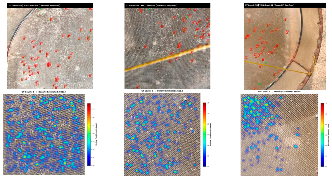
To examine the model’s failure modes under complex aquaculture conditions, several representative cases are analyzed in Figure 9. Although the overall framework remains stable in most scenarios, performance degrades under several types of interference. First, reflections from the metal frame, occlusion by suspension ropes, and visually similar suspended objects can confuse the detection branch, leading to false positives or missed residual feed pellets. Second, suspended particles and organic flocs in turbid water may produce weak density responses even in regions without residual feed, causing overestimation after spatial accumulation. Third, when multiple sources of interference occur simultaneously, such as suspended matter combined with feed-tray frame occlusion, the detection branch may generate false bounding boxes while the density branch produces abnormal high-response regions at the same locations. In such cases, the two branches do not effectively compensate for each other, resulting in larger prediction errors.
These failure cases reveal the main limitations of the current model and suggest several directions for further improvement. Future work could explore a cross-branch constraint mechanism that links detection boxes with density-map responses, allowing false background activations to be suppressed more effectively and improving robustness under complex aquaculture conditions.
4.8. Discussion
The improved performance of YOLO-SPD-LSK-DGD can be attributed to the complementary roles of feature preservation, background suppression, boundary regression, and density modeling. Because residual feed pellets occupy only a few pixels, their features are easily weakened during downsampling. The ablation results show that SPD-Conv improves both mAP50 and APsmall, suggesting that preserving spatial details during feature extraction is important for tiny-object detection. C2f-LSK further enhances detection by adapting the receptive field to different spatial contexts, helping the network distinguish residual feed pellets from structured interference such as feed-tray grids and water-surface reflections. The gains obtained from the combined Focaler-CIoU and NWD loss also indicate that more stable boundary regression is beneficial for small, densely clustered targets, where even slight coordinate shifts can lead to substantial changes in IoU.
The comparison results suggest that the proposed modifications are well matched to the characteristics of residual-feed images. Although several YOLO variants maintain high inference speeds, their performance declines when feed pellets are extremely small or densely clustered. The proposed model achieves an mAP50 of 0.9231 while maintaining an inference speed of 100.8 FPS, showing that targeted improvements in feature preservation and background suppression can be more effective for this task than simply increasing model complexity. Its strong APsmall performance further confirms the model’s suitability for detecting tiny residual-feed pellets.
The density branch complements detection-based counting by providing information about how residual feed is distributed across the tray. Feed trays with similar pellet counts may show very different spatial patterns, and localized accumulation may therefore require different feeding adjustments from uniformly dispersed residues. By sharing backbone features, the two branches provide both pellet locations and continuous density information within a single network. The dynamic Gaussian strategy also improves density regression performance, increasing R2 from 0.8616 with a fixed Gaussian kernel to 0.9004 and reducing RMSE from 2.9945 to 2.7012. This improvement suggests that adjusting the Gaussian bandwidth according to local nearest-neighbor distances provides a better representation of changes in pellet spacing than using a fixed kernel.
Performance across different stacking conditions also reveals a clear decline as residual-feed density increases. The MAE rises from 1.0497 for uniformly dispersed pellets to 2.2872 under local accumulation and 5.0227 under severe overlap, while R2 decreases from 0.7645 to about 0.69. This decline is likely related to severe occlusion and the merging of neighboring responses, which make pellet boundaries more difficult to distinguish for both branches. The relative error of local density peaks also varies differently from the overall counting error. The larger peak error observed in sparse scenes suggests that local density estimation is affected not only by pellet count but also by small spatial shifts between the predicted and ground-truth Gaussian responses. These findings indicate that both global counting accuracy and local density characteristics should be considered when evaluating the density branch.
Several limitations should be noted. The dataset was collected from a relatively limited range of shrimp farming environments, and the model still requires further validation across different pond structures, water turbidities, lighting conditions, feed sizes, and camera settings. Suspended particles, frame reflections, and severe pellet adhesion may still lead to false detections or abnormal density responses, as shown in the failure cases. In addition, the current density map reflects the spatial distribution of pellet centers rather than the actual mass of residual feed. Future work could therefore explore consistency constraints between the detection and density branches, incorporate temporal information from consecutive feed-tray images, and establish a calibration relationship between visual density and residual-feed mass. These developments may further support integration with automated feeding systems for closed-loop feeding control in practical shrimp farming.
5. Conclusions and Future Work
Intensive shrimp farming requires accurate monitoring of uneaten feed, which is typically small, densely clustered, and difficult to characterize using conventional vision-based methods. This study proposes YOLO-SPD-LSK-DGD, an end-to-end network that integrates object detection with spatial density estimation. The backbone combines SPD-Conv and C2f-LSK modules to preserve fine-grained features during downsampling and reduce interference from complex backgrounds. A dynamic Gaussian representation with adaptive neighborhood constraints is introduced to generate continuous density maps together with detection bounding boxes. In addition, a hybrid loss combining Focaler-CIoU and NWD is used to improve bounding-box regression for densely distributed small targets. Experiments on a self-collected shrimp feed-tray dataset showed that the proposed model achieved an mAP50 of 0.9231 for object detection, an R2 of 0.9004 for density regression, and an inference speed of 100.8 FPS. These results demonstrate that the model can simultaneously localize residual feed pellets and characterize their spatial distribution while maintaining real-time inference performance.
Although YOLO-SPD-LSK-DGD achieves strong overall performance, its robustness can still be improved under challenging conditions such as intense metal reflections and highly turbid water. Future work will investigate stronger consistency between detection boxes and density maps to reduce background interference in complex scenes. Inspired by studies on fish behavior recognition [29,30], it will also explore the use of shrimp behavioral information, including group density and activity, to support closed-loop feeding strategies.The detection head will also be extended to multi-class recognition so that residual feed pellets, fecal residues, and foreign impurities can be distinguished using class-adaptive loss functions. In addition, unsupervised and semi-supervised domain adaptation will be explored to reduce annotation costs when transferring the model across different water-quality conditions and feed-tray configurations.Finally, automated machine learning will be adopted to explore multi-task neural architecture search, so as to develop an intelligent aquaculture monitoring system that supports pellet counting, behavioral analysis and growth-performance evaluation.
Author Contributions
Xingze Zhang: Conceptualization, Methodology, Software, Data curation, Formal analysis, Investigation, Validation, Visualization, Writing – original draft, Writing – review and editing. Peiyu Tang: Software, Investigation, Formal analysis, Validation. Nannan Zhao: Supervision, Methodology, Writing – review and editing.
Funding
This research did not receive any specific grant from funding agencies in the public, commercial, or not-for-profit sectors.
Institutional Review Board Statement
The present study primarily focuses on the image acquisition and computer-vision analysis of uneaten feed residues on feeding trays in an aquaculture environment. During data collection, we only photographed the residual feed on the feeding trays for subsequent image annotation, model training, and evaluation. No experimental procedures, invasive operations, treatments, or interventions were performed on live shrimp for the purposes of this study.
Data Availability Statement
The dataset used in this study was collected by the authors and has not been deposited in a public repository. The data are available from the corresponding author upon reasonable request.
Acknowledgments
The authors would like to thank the staff who assisted with field data collection at the aquaculture site, the aquaculture enterprise that provided access to the shrimp ponds, feed trays, and experimental facilities, and the personnel who supported equipment installation and on-site experimental setup. Their assistance contributed significantly to the successful completion of this study.
Conflicts of Interest
The authors declare no conflict of interest.
Declaration of generative AI and AI-assisted technologies in the manuscript preparation process: During the preparation of this work, the authors used ChatGPT (OpenAI) to assist with English language refinement and grammatical improvement. After using this tool, the authors reviewed and edited the content as needed and take full responsibility for the content of the published article.
References
- Saha, S.; Rajib, R. H.; Kabir, S. IoT based automated fish farm aquaculture monitoring system[C]//2018 International Conference on Innovations in Science, Engineering and Technology (ICISET); IEEE; Volume 2018, pp. 201–206.
- Simbeye, D. S.; Zhao, J.; Yang, S. Design and deployment of wireless sensor networks for aquaculture monitoring and control based on virtual instruments[J]. Comput. Electron. Agric. 2014, 102, 31–42. [Google Scholar] [CrossRef]
- Sharif, M. G. Smart peripatetic food feeding system for aquafarm[C]//2024 IEEE International Conference on Interdisciplinary Approaches in Technology and Management for Social Innovation (IATMSI). IEEE 2024, 2, 1–5. [Google Scholar]
- Imai, T.; Arai, K.; Kobayashi, T. Smart aquaculture system: a remote feeding system with smartphones[C]//2019 IEEE 23rd international symposium on consumer technologies (ISCT); IEEE, 2019; pp. 93–96. [Google Scholar]
- Hu, X.; Liu, Y.; Zhao, Z.; et al. Real-time detection of uneaten feed pellets in underwater images for aquaculture using an improved YOLO-V4 network[J]. Comput. Electron. Agric. 2021, 185, 106135. [Google Scholar] [CrossRef]
- Gao, G.; Gao, J.; Liu, Q.; et al. A survey of deep learning methods for density estimation and crowd counting[J]. Vicinagearth 2025, 2, 2. [Google Scholar] [CrossRef]
- Sindagi, V. A.; Patel, V. M. A survey of recent advances in cnn-based single image crowd counting and density estimation[J]. Pattern Recognit. Lett. 2018, 107, 3–16. [Google Scholar] [CrossRef]
- Idrees, H.; Tayyab, M.; Athrey, K.; et al. Composition loss for counting, density map estimation and localization in dense crowds[C]//European Conference on Computer Vision; Springer International Publishing: Cham, 2018; pp. 544–559. [Google Scholar]
- Liu, Y.; Sun, P.; Wergeles, N.; et al. A survey and performance evaluation of deep learning methods for small object detection[J]. Expert Syst. With Appl. 2021, 172, 114602. [Google Scholar] [CrossRef]
- Cheng, G.; Yuan, X.; Yao, X.; et al. Towards large-scale small object detection: Survey and benchmarks[J]. IEEE Trans. Pattern Anal. Mach. Intell. 2023, 45(11), 13467–13488. [Google Scholar] [CrossRef] [PubMed]
- Bochkovskiy, A.; Wang, C. Y.; Liao, H. Y. M. Yolov4: Optimal speed and accuracy of object detection[J]. arXiv 2020, arXiv:2004.10934. [Google Scholar]
- Wang, S.; Xu, M.; Sun, Y.; et al. Improved single shot detection using DenseNet for tiny target detection[J]. Concurr. Comput. Pract. Exp. 2023, 35(2), e7491. [Google Scholar] [CrossRef]
- Ju, M.; Luo, J.; Zhang, P.; et al. A simple and efficient network for small target detection[J]. IEEE Access 2019, 7, 85771–85781. [Google Scholar] [CrossRef]
- Sunkara, R.; Luo, T. No more strided convolutions or pooling: A new CNN building block for low-resolution images and small objects[C]//Joint European conference on machine learning and knowledge discovery in databases; Springer Nature Switzerland: Cham, 2022; pp. 443–459. [Google Scholar]
- Hsu, P. H.; Lee, P. J.; Bui, T. A. YOLO-SPD: Tiny objects localization on remote sensing based on You Only Look Once and Space-to-Depth Convolution[C]//2024 IEEE International Conference on Consumer Electronics (ICCE); IEEE, 2024; pp. 1–3. [Google Scholar]
- Li, Y.; Hou, Q.; Zheng, Z.; et al. Large selective kernel network for remote sensing object detection[C]//2023 IEEE/CVF International Conference on Computer Vision (ICCV); IEEE, 2023; pp. 16748–16759. [Google Scholar]
- Li, Y.; Li, X.; Dai, Y.; et al. LSKNet: A foundation lightweight backbone for remote sensing[J]. Int. J. Comput. Vis. 2025, 133(3), 1410–1431. [Google Scholar] [CrossRef]
- Zhou, D.; Fang, J.; Song, X.; et al. Iou loss for 2d/3d object detection[C]//2019 international conference on 3D vision (3DV); IEEE, 2019; pp. 85–94. [Google Scholar]
- Xu, C.; Wang, J.; Yang, W.; et al. Detecting tiny objects in aerial images: A normalized Wasserstein distance and a new benchmark[J]. ISPRS J. Photogramm. Remote Sens. 2022, 190, 79–93. [Google Scholar] [CrossRef]
- Zhang, H.; Zhang, S. Focaler-iou: More focused intersection over union loss[J]. arXiv 2024, arXiv:2401.10525. [Google Scholar]
- Spampinato, C.; Giordano, D.; Di Salvo, R.; et al. Automatic fish classification for underwater species behavior understanding. In Proceedings of the first ACM international workshop on Analysis and retrieval of tracked events and motion in imagery streams, 2010; pp. 45–50. [Google Scholar]
- Zhang, Y.; Yang, Q. A survey on multi-task learning[J]. IEEE Trans. Knowl. Data Eng. 2022, 34(12), 5586–5609. [Google Scholar] [CrossRef]
- Weyler, J.; Milioto, A.; Falck, T.; et al. Joint plant instance detection and leaf count estimation for in-field plant phenotyping[J]. IEEE Robot. Autom. Lett. 2021, 6(2), 3599–3606. [Google Scholar] [CrossRef]
- Liu, C.; Weng, X.; Mu, Y. Recurrent attentive zooming for joint crowd counting and precise localization[C]//2019 IEEE/CVF conference on computer vision and pattern recognition (CVPR); IEEE, 2019; pp. 1217–1226. [Google Scholar]
- Care, A.; Carli, R.; Dalla Libera, A.; et al. Kernel methods and gaussian processes for system identification and control: A road map on regularized kernel-based learning for control[J]. IEEE Control Syst. Mag. 2023, 43(5), 69–110. [Google Scholar] [CrossRef]
- Valloli, V. K.; Mehta, K. W-net: Reinforced u-net for density map estimation[J]. arXiv 2019, arXiv:1903.11249. [Google Scholar]
- Jiang, P.; Ergu, D.; Liu, F.; et al. A Review of Yolo algorithm developments[J]. Procedia Comput. Sci. 2022, 199, 1066–1073. [Google Scholar] [CrossRef]
- Terven, J.; Córdova-Esparza, D. M.; Romero-González, J. A. A comprehensive review of yolo architectures in computer vision: From yolov1 to yolov8 and yolo-nas[J]. Mach. Learn. Knowl. Extr. 2023, 5(4), 1680–1716. [Google Scholar] [CrossRef]
- Abangan, A. S.; Kopp, D.; Faillettaz, R. Artificial intelligence for fish behavior recognition may unlock fishing gear selectivity[J]. Front. Mar. Sci. 2023, 10, 1010761. [Google Scholar] [CrossRef]
- Wang, G.; Muhammad, A.; Liu, C.; et al. Automatic recognition of fish behavior with a fusion of RGB and optical flow data based on deep learning[J]. Animals 2021, 11(10), 2774. [Google Scholar] [CrossRef] [PubMed]
- Xu, C.; Wang, Z.; Du, R.; et al. A method for detecting uneaten feed based on improved YOLOv5[J]. Comput. Electron. Agric. 2023, 212, 108101. [Google Scholar] [CrossRef]
- Hu, H.; Tang, C.; Shi, C.; et al. Detection of residual feed in aquaculture using YOLO and Mask RCNN[J]. Aquac. Eng. 2023, 100, 102304. [Google Scholar] [CrossRef]
- Zhang, Y.; Zhou, D.; Chen, S.; et al. Single-image crowd counting via multi-column convolutional neural network[C]//2016 IEEE Conference on Computer Vision and Pattern Recognition (CVPR); IEEE, 2016; pp. 589–597. [Google Scholar]
- Song, Q.; Wang, C.; Jiang, Z.; et al. Rethinking counting and localization in crowds: A purely point-based framework[C]//2021 IEEE/CVF International Conference on Computer Vision (ICCV); IEEE, 2021; pp. 3345–3354. [Google Scholar]
- Zhang, L.; Li, Y.; Li, Z.; et al. Estimating residual bait density using hybrid dilated convolution and attention multi-scale network[J]. Trans. Chin. Soc. Agric. Eng. 2024, 40(14), 137–145. [Google Scholar]
- Xi, M.; Rahman, A.; Nguyen, C.; et al. Smart headset, computer vision and machine learning for efficient prawn farm management[J]. Aquac. Eng. 2023, 102, 102339. [Google Scholar] [CrossRef]
- Du, Z.; Cui, M.; Wang, Q.; et al. Feeding intensity assessment of aquaculture fish using Mel Spectrogram and deep learning algorithms[J]. Aquac. Eng. 2023, 102, 102345. [Google Scholar] [CrossRef]
- Wang, Z.; Qian, R.; Deng, H.; et al. Precise feeding technology for outdoor pond aquaculture based on detection and counting method[J]. Aquac. Eng. 2025, 111, 102588. [Google Scholar] [CrossRef]
- Colt, J.; Tchobanoglous, G.; Johnson, R. B. Measurement of settling velocities of feeds and fecal solids in aquacultural applications: A critical review[J]. Aquac. Eng. 2025, 111, 102548. [Google Scholar] [CrossRef]
- Føre, M.; Alver, M. O.; Alfredsen, J. A.; et al. Digital Twins in intensive aquaculture: Challenges, opportunities and future prospects[J]. Comput. Electron. Agric. 2024, 218, 108676. [Google Scholar] [CrossRef]
Figure 1.
Overall Structure Diagram.
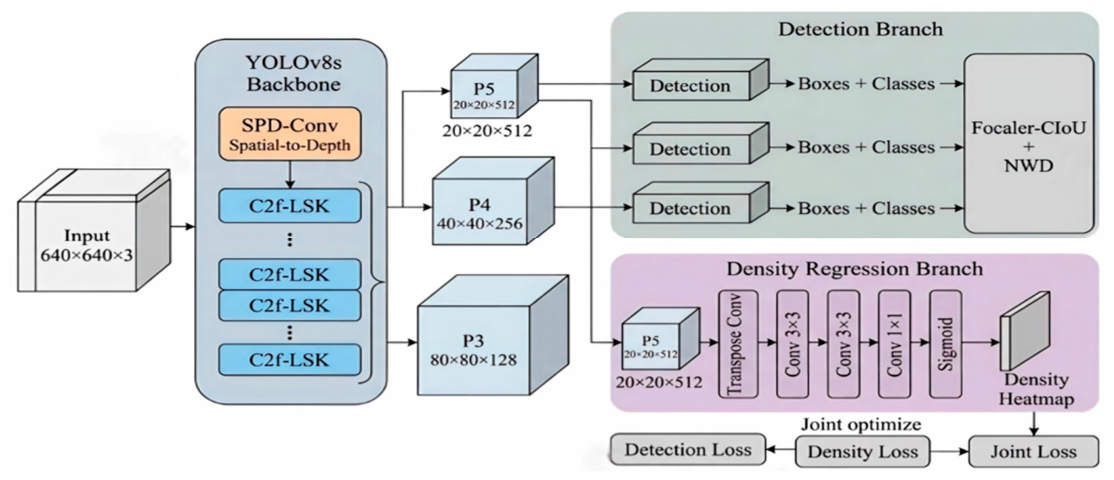
Figure 5.
Training convergence and performance metrics of the YOLO model.
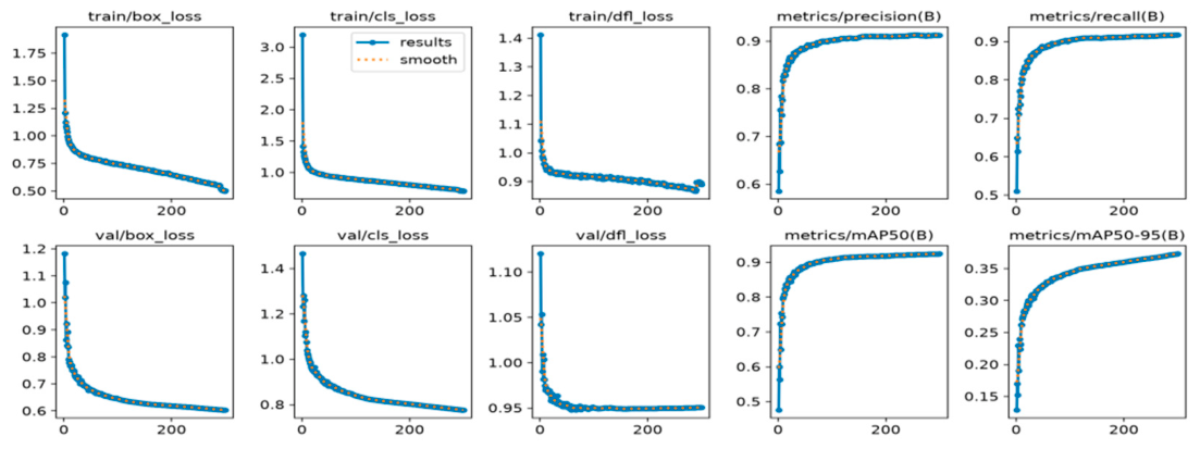
Figure 6.
YOLO Model Detection Performance and Confusion Matrix Evaluation Chart.
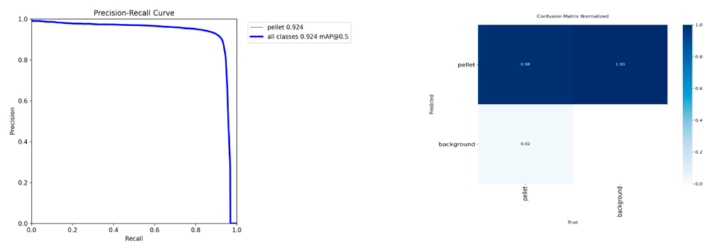
Figure 7.
Density estimation performance and training convergence.
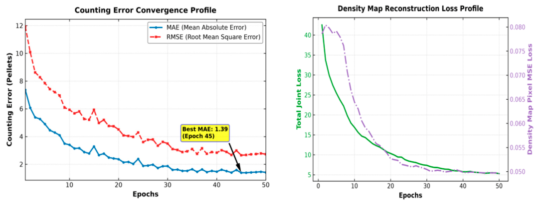
Figure 8.
Comparison of Density Heatmap Evolution.
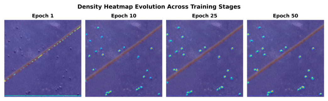
Figure 9.
Visualization of failure cases under complex aquaculture conditions.
Disclaimer/Publisher’s Note: The statements, opinions and data contained in all publications are solely those of the individual author(s) and contributor(s) and not of MDPI and/or the editor(s). MDPI and/or the editor(s) disclaim responsibility for any injury to people or property resulting from any ideas, methods, instructions or products referred to in the content. |
© 2026 by the authors. Licensee MDPI, Basel, Switzerland. This article is an open access article distributed under the terms and conditions of the Creative Commons Attribution (CC BY) license (http://creativecommons.org/licenses/by/4.0/).
Copyright: This open access article is published under a Creative Commons CC BY 4.0 license, which permit the free download, distribution, and reuse, provided that the author and preprint are cited in any reuse.