

Submitted:
28 September 2026
Posted:
30 September 2026
You are already at the latest version
Abstract
Sand scorpions are a useful model for deriving principles of navigation by familiarity using a local sensor. Immediately after digging its burrow, a sand scorpion performs a series of learning walks that may facilitate the acquisition of home-directed tastes and touches via its midventral pectines. Later, during subsequent homebound journeys, the scorpion repeatedly compares current tastes and textures to the memories acquired via learning walks, using this information to step in the direction of the most familiar memory until it reaches its home. Previously, we have created computer simulations to show proof-of-concept of this navigation process. My goal here is to illustrate the idea with a simple, easily replicated robotic toy “scorp-car” that navigates based on the familiarity algorithm. I expect this robot to not only shed light on scorpion sensory biology but also inspire translational applications involving autonomous navigation within human-built environments.
Keywords:
navigation
; robot
; pectines
; homing
1. Introduction
The concept of Navigation by Familiarity is deceptively simple. As such, I decided to design an inexpensive robotic car that navigates by familiarity so that anyone can reproduce and interact with the robot to “feel” how the process works. The specific process the robot emulates is termed Navigation by Familiarity with a Local Sensor (NFLS for short) [1], which was inspired by scorpions that navigate to their home burrows with the aid of their exquisite midventral taste/touch organs called pectines.
Let me review some background about what we know about sand scorpion navigation and their pectines. These scorpions dig burrows in the sand and are largely faithful to these burrows when returning from hunting excursions [2,3,4,5]. These animals appear to be capable of path integration [6] to relocate their home burrow and perform putative learning walks immediately after digging their burrows [7]. We suspect that they use dense fields of peg sensilla on their pectines [8,9,10,11,12] to gather home-directed information during path integration (of which learning walks could be considered a subset [13,14,15]) and that they later use this information to return to their burrows via familiarity navigation [1,16,17,18,19,20,21,22,23,24].
The paired pectines (Figure 1) are chemo-tactile organs that sweep the ground as the animal walks, collecting both taste and tactile information. The organs are divided into a species-specific number of teeth, and the distal, ground-directed tooth surfaces are adorned with a dense field of microscopic structures called peg sensilla (aka "pegs"). Each peg contains a population (~10) of chemo-sensitive neurons and a single mechano-sensitive neuron [3,8,9,12]. Although pegs are responsive to numerous organic chemo-stimulants [25], their response profiles are similar to each other [26,27]. Furthermore, chemosensory responses are detectable only when the peg tips are within ~20 microns of the stimulant [28,29].
For two reasons, I suspect that the summation of all the peg inputs on each tooth forms the basic unit of information from the pectines. First, the central projections from the peg sensilla are topographically organized by tooth in the central nervous system [3,30,31]. Second, we have used computer simulations to vary the sensory resolution of pectines by dividing the sensory "reporting" of each tooth into subregions ranging in number from zero to 32; we found no difference in navigation performance [21]. I used these insights to guide the development of my robotic car’s sensor.
Actual scorpions use their pectines to transduce minuscule amounts of chemicals and microscopic textural nuances from the ground as they walk. Since it is not currently possible to transduce such microscopic stimuli for robotic guidance, I opted to use a downward-facing camera and a patterned floor as proxies for pecten function [1,18,19,20,21]. I also used only simple, readily available components to develop my robotic car so that others can build their own and test the ideas for themselves. This vehicle navigates across patterned surfaces using only the NFLS process and should help readers better understand the idea of familiarity navigation, provide additional support to the idea that scorpions may be using NFLS to navigate, and perhaps inspire its use in translational applications.
2. Materials and Methods
2.1. Visualization of NFLS Algorithm as Applied to Scorpions
The mathematical expression of the NFLS algorithm is provided in the supplementary materials. I also created two animations to help explain how the NFLS algorithm works. The first animation (Figure 2; Video S1) includes working memory as the scorpion navigates toward a goal. The animal/agent first acquires a set of glimpses during its initial goal-directed journey ("Initial Journey" or IJ; blue dots in Figure 2). The rectangle of the sensor representing the pectines acquires and stores the average gray scale value for each of the 40 pectinal teeth. In the Figure 2 example, 40 IJ steps were taken, and each step’s glimpse was stored as the leftmost column in the 40 groupings shown in the IJ Memory at the bottom of the figure. The agent was then placed near the start of the IJ, facing parallel to the direction of the IJ path. Its pectines then made a rotational saccade of +35o at 5o increments (these rotational glimpses are shown in the middle columns of IJ memory below). [Note that for the robot car, I used a reduced rotational saccade of +14o at 2o increments.] The absolute differences (tooth by tooth) between the IJ memories and the current rotational glimpses are shown in the rightmost columns of the IJ groupings with the sum of these absolute differences (SAD) shown below the columns. The glimpse angle that yields the minimum of these SADs is selected and the agent steps forward in that direction and repeats the process. The second animation (Video S2) shows a longer example using a curvy IJ path. In that example, I removed the depiction of the IJ memory and showed only the graphs corresponding to the minimum SAD as a function of rotation angle and IJ index.
2.2. Robotic Car Build
I selected the OSOYOO 2WD Robot Car Starter Kit for Arduino as the basic robotic car chassis. I chose this platform because of its affordability and because I could mount a downward-facing camera (to simulate the pectines) near the pivot point of the two drive wheels of the three-wheeled vehicle (the rear wheel was a small passive universal wheel). The car was designed to travel with the small universal wheel in front and the two large drive wheels in the back. I opted to modify the software to run the car in reverse and mount the camera so that its focus was close to the axis of the large wheels to better mimic the location of scorpion pectines close to the pivot point of the scorpion body relative to its eight legs.
The main parts of the OSOYOO kit consisted of a chassis, an Arduino board, a motor shield, a motor driver, and right and left motors connected to the right and left wheels (Figure 3). I modified the car in several important ways. First, through testing, I discovered that the TT-style gearbox motors supplied with the kit did not produce the slow, deliberate wheel rotations needed for NFLS control. As such, I exchanged the TT-style motors with metal DC geared motors equipped with with encoders (CQRobot: 270:1 metal DC gear motor 37D x 72.5L mm 6V/12V with 64 CPR encoder). To mount the motors, I cut and affixed a rectangular aluminum plate (16.3 x 3.8 x 0.3 cm) to the bottom of the Plexiglas chassis below the motor driver and then mounted the new metal motors at either end with their axles protruding from the sides of the car. I used a small round file to carefully ream the central holes in the plastic hubs of the kit’s provided wheels so that they fit snugly on the 6mm diameter motor axles. I then cut a rectangular hole (3.6 cm x 1.6 cm) in the Plexiglas chassis just in front of the aluminum plate and used four 6.5 cm long bolts (along with hex nuts) to support a wooden platform (14.0 x 4.0 x 0.5 cm) at 5.0 cm above this hole. I cut a 2.5 cm diameter hole in the wooden platform and mounted a USB Microscope camera with an LED light source (ViTiny UM02 Handheld USB Digital Microscope for PC, ViTiny USA) so that its lens faced downward through this circular hole and down towards the substrate through the rectangular hole. The camera’s lens was 10.5 cm above the substrate. I used velcro tape to add a Raspberry Pi board (Raspberry Pi Zero 2W (Wireless/Bluetooth) 2021 (RPi Zero 2W)) to the rear of the car’s chassis and a USB hub (SMAYS Micro USB to Ethernet Adapter for Raspberry Pi Zero) to the front of the chassis.
The camera was connected to the USB hub, which, in turn, was connected to the micro-USB port on the Raspberry Pi (Figure 4A); the USB hub was also connected to the Arduino. I found that powering the car quickly drained the supplied battery source. So, for testing, I connected the car to AC power by using appropriate AC adapters to deliver power to the Arduino (adapter: 12V, 1.5A output) and Pi (adapter: 5V, 1.4A output). Since I did not use the car’s battery source, I removed its housing from the car to free up space for the raspberry Pi.
2.3. Modeling the Pectines
I modeled the pectines by using the downward-facing camera to capture a grayscale rectangular visual patch (1370 pixels wide, 70 pixels deep) that was then parsed to 40 teeth by averaging contiguous blocks (Figure 1B). The 40 pectinal teeth were arranged as a continuous bar that could be rotated +14o at 2o increments by rotating the robot car accordingly (Figure 4B).
2.4. Python Scripts and Arduino Sketch
To communicate with the Raspberry PI, I used my cell phone (Motorola Moto G Stylus) to establish a local hotspot that I connected to both my laptop and the Pi. I used the laptop’s Terminal, a secure shell (SSH), and the GNU Nano editor to paste my Python script to access the camera, process and save images and vectors, and communicate with the Arduino to control the car’s motion. Python scripts and output files were saved on a 32 GB microSD card (onn brand). To configure the car’s motor commands, I connected the car to my laptop and flashed the appropriate sketch using Arduino IDE 2.3.10. The IJ capture script, the SJ navigational script, and the Arduino sketch are available in the Supplementary Materials. I used the Unix scp command to transfer output files over SSH from the Pi to my laptop for subsequent analysis in Python.
2.5. Use of GenAI
I used GenAI (Microsoft Copilot) to assist and guide the selection, assembly, and programming of the robot car. I also used it to generate the NFLS mathematical equations shown in the supplementary materials section.
3. Results
I ran some preliminary tests to get a sense of the robotic car’s precision of movement and to check its processing of the camera’s images to 40-unit vectors. The car was run forward in a straight path over a piece of white printer paper containing printed block letters (Figure 5). The car made 60 forward steps, pausing for several milliseconds to acquire an image, crop it to a 1370 x 70 pixel rectangle, down-sample it to 40 unsigned 8-bit integers (uint8), and store it in memory. The memory matrix of the 60 samples of 40-unit vectors is displayed at right in (Figure 5). For the most part, the car’s forward movement was straight, with a very slight veer to the left. Since each 40-unit vector is 40 bytes, the memory required for this 60 step excursion was 2.4 KB.
I next began tests on a terrazzo floor landscape. I created the test landscape by using my cell phone’s camera to capture a photo of a patch of terrazzo floor in one of my university’s buildings (first floor, Richards Hall, University of Oklahoma). I converted the photo to grayscale and printed the image on heavyweight paper to a final size of 380 mm wide by 300 mm tall. I used the IJ capture script to run the car 80 steps forward, followed by 80 steps backward (Figure 6A) to capture a total of 160 40-unit image vectors (Figure 6B). I cross-correlated the 160 vectors to generate the plot shown in Figure 6C. The "X" pattern in the plot not only provides a sense of the strong information difference between a given vector and vectors captured in other regions of the terrazzo landscape, but also shows that the car accurately tracks back close to the forward captured glimpses.
To further assess the information available for familiarity navigation, I calculated the absolute sum of the cell-by-cell differences (aka SAD) of 40-unit vectors compared to other vectors in two ways. First, I ran an IJ script where the car made 80 forward steps, generating a 40-unit vector with each step. The car traveled a total of 25 cm, so each step was approximately 0.3 cm (25 cm / 80 steps). The results of this test are shown in Figure 7A. The SAD plot shows that the width of the trough at p50 (~0.25 SAD) is about 6 steps (+3 steps from each focal vector) or ~1.8 cm. Second, I assessed SAD for 20 SJ steps in which the rotational vectors (from -14o to +14o at 2o increments) were compared to the 0o, forward facing vector. The width of the trough at p50 SAD (~1.0) is about 4 degrees (+2 o from each forward-facing vector).
Next, I looked at the potential NFLS information available to an agent compared to the actual performance of the scorp-car across a patch of the terrazzo landscape. The length of the IJ in both cases was 12 cm, and 47 forward steps were made in both cases for ~0.26 cm per step. Figure 8 depicts the potential information available, while Figure 9 shows the performance of the scorp-car run over the same patch.
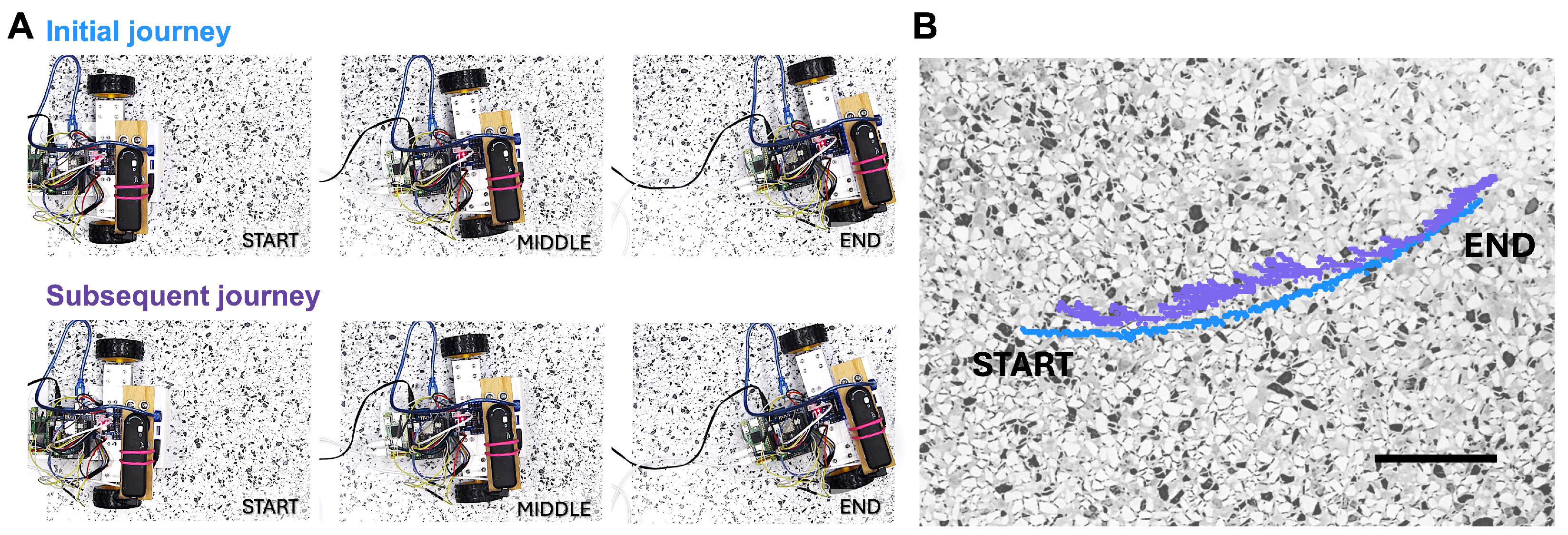
Finally, I videotaped from above a run of the scorp-car in relation to a slightly curved IJ. I wrote a Python script to automatically track the position of a red illuminated LED on the car’s motor driver, which was positioned slightly to the left of the car’s midline and slightly behind the wheel axis. The results of this run are shown in Figure 10, and a video of the run is available in the Supplementary Materials. As can be seen in the plot of Figure 10B, the car begins a little away from the IJ path, but appears to latch onto it near the end of the run.
4. Discussion
While the scorp-car described in this manuscript is far from a final product, it shows that navigation by familiarity with a local sensor is feasible. This study provides additional proof-of-concept that a robotic car can navigate via NFLS (akin to how we think a scorpion uses its pectines in navigation).
I hope the elegance of the NFLS algorithm is apparent and appreciated. The scorp-car’s navigation emerges from purely local comparisons between the current sensory input and a stored matrix of familiar views, without requiring a global map or having to remember sequences. This model demonstrates the simplicity of the NFLS process and the compactness of the requisite memory. For example, navigating a path the size of a typical sand scorpion’s home range (about 2 m) requires only ~30 KB of memory (at 0.26 cm and 40 bytes per step). It would require only ~15 MB to navigate the length of a football field.
This car should provide a baseline for what is possible, even with relatively simple, affordable components. In all, before tax and shipping, the car cost less than $170 in US dollars (OSOYOO robot car kit $40.99; DC geared motors $15.99; Raspberry Pi $38.99; USB microscope camera similar to the discontinued Vitany model I used $36.99; microSD card $16.92; USB hub $13.99; various hardware < $5.00).
I am currently making several improvements to the scorp-car’s design. I am refining the car’s rotational saccade accuracy and working to equip the car with a reliable onboard power supply so I do not have to tether the car to an AC power source. This will allow me to test the car’s navigation over longer, curvier paths and over various landscapes. For example, I predict poor performance over a landscape of random pixels. I think both the blobbiness and the randomness (i.e., coherent stochastic texture) of the terrazzo floor patterns are crucial for robust familiarity navigation. Also, instead of rotating the entire car for each saccade, I am exploring capturing a larger camera image and digitally extracting and rotating glimpses to form the SJ saccades. This change may provide more rotational precision without relying on balanced control of the car’s two motors.
It would also be great to find and test a platform that allows side-to-side movement to add translational information [21] to the rotational information used in the current version. Our previous simulations have shown that translational information is very useful for moving an agent towards the IJ’s catchment influence. Along these lines, I think a low-flying drone with precise motion control would be a great direction to pursue.
There is enormous potential for self-navigating robots that do useful things in institutions of various sorts, and terrazzo floors are plentiful in many built environments, such as airports, hospitals, stores, and university hallways. Or, if terrazzo flooring is not available, a similar car could be engineered that instead (or in addition) uses randomized patterns on the ceiling. Delivering medications to patient rooms, collecting items from store shelves, and transporting people and luggage to terminal gates are all feasible applications for NFLS technology.
Supplementary Materials
The following supporting information can be downloaded at the website of this paper posted on Preprints.org. NOTE: Repositories of our Python scripts and Arduino sketches will be provided upon publication. All additional data are available in the main text or in the supplementary materials.
Funding
This research received no external funding.
Informed Consent Statement
Not applicable.
Data Availability Statement
Data is contained within the article.
Acknowledgments
I thank Mariëlle Hoefnagels for editorial review, George Martin for engineering assistance, the OU School of Biological Sciences for facilities support, and OU Presidential Teaching Fellow in Honors funds for research materials. Finally, I appreciate the help of Microsoft Copilot in developing the mathematical expressions and python code used in NFLS.
Conflicts of Interest
The author declares no conflicts of interest.
References
- Musaelian, A.; Gaffin, D.D. High-throughput simulations indicate feasibility of navigation by familiarity with a local sensor such as scorpion pectines. bioRxiv 2020, 2020.06.17.156612. [Google Scholar] [CrossRef]
- Polis, G.A.; McReynolds, C.N.; Ford, R.G. Home range geometry of the desert scorpion Paruroctonus mesaensis. Oecologia 1985, 67, 273–277. [Google Scholar] [CrossRef] [PubMed]
- Brownell, P. Sensory ecology and orientational behaviors. In Scorpion Biology and Research.; Oxford University Press, 2001; pp. 159–183. [Google Scholar]
- Gaffin, D. In situ infrared videography of sand scorpion nighttime surface activity. Euscorpius 2011, 2011, 1–13. [Google Scholar] [CrossRef]
- Gaffin, D.D.; Curry, C.M. Arachnid navigation – a review of classic and emerging models. J. Arachnol. 2020, 48, 1–25. [Google Scholar] [CrossRef]
- Prévost, E.D.; Stemme, T. Non-visual homing and the current status of navigation in scorpions. Anim. Cogn. 2020, 23, 1215–1234. [Google Scholar] [CrossRef] [PubMed]
- Gaffin, D.D.; Muñoz, M.G.; Hoefnagels, M.H. Evidence of learning walks related to scorpion home burrow navigation. J. Exp. Biol. 2022, 225, jeb243947. [Google Scholar] [CrossRef] [PubMed]
- Foelix, R.F.; Müller-Vorholt, G. The fine structure of scorpion sensory organs. II.Pecten sensilla. Bull. Br. Arachnol. Soc. 1983, 6, 68–74. [Google Scholar]
- Ivanov, V.; Balashov, Y. The structural and functional organization of the pectine in a scorpion Buthus eupeus Koch (Scorpiones, Buthidae) studied by electron microscopy; The fauna and ecology of Arachnida., Ed.; Trudy Zoological Institute: Leningrad, 1979; Vol. 85, pp. 73–87. [Google Scholar]
- Cloudsley-Thompson, J. L.X.V.I.I. On the function of the pectines of scorpions. Ann. Mag. Nat. Hist. 1955, 8, 556–560. [Google Scholar] [CrossRef]
- Wolf, H. Scorpions pectines – idiosyncratic chemo- and mechanosensory organs. Arthropod Struct. Dev. 2017, 46, 753–764. [Google Scholar] [CrossRef] [PubMed]
- Gaffin, D.; Brownell, P. Chemosensory behavior and physiology. In Scorpion Biology and Research; Oxford University Press, 2001; pp. 184–203. [Google Scholar]
- Ortega-Escobar, J.; Hebets, E.A.; Bingman, V.P.; Wiegmann, D.D.; Gaffin, D.D. Comparative biology of spatial navigation in three arachnid orders (Amblypygi, Araneae, and Scorpiones). J. Comp. Physiol. A 2023. [Google Scholar] [CrossRef] [PubMed]
- Wolf, H. Odometry and insect navigation. J. Exp. Biol. 2011, 214, 1629–1641. [Google Scholar] [CrossRef] [PubMed]
- Zeil, J.; Fleischmann, P.N. The learning walks of ants (Hymenoptera: Formicidae). Myrmecol. News 2019, 29, 93–110. [Google Scholar] [CrossRef]
- Baddeley, B.; Graham, P.; Philippides, A.; Husbands, P. Holistic visual encoding of ant-like routes: navigation without waypoints. Adapt. Behav. 2011, 19, 3–15. [Google Scholar] [CrossRef]
- Baddeley, B.; Graham, P.; Husbands, P.; Philippides, A. A model of ant route navigation driven by scene familiarity. PLoS Comput. Biol. 2012, 8, e1002336. [Google Scholar] [CrossRef] [PubMed]
- Gaffin, D.D.; Dewar, A.; Graham, P.; Philippides, A. Insect-inspired navigation algorithm for an aerial agent using satellite imagery. PLoS ONE 2015, 10, e0122077. [Google Scholar] [CrossRef] [PubMed]
- Gaffin, D.D.; Brayfield, B.P. Autonomous visual navigation of an indoor environment using a parsimonious, insect inspired familiarity algorithm. PLoS ONE 2016, 11, e0153706. [Google Scholar] [CrossRef] [PubMed]
- Gaffin, D.D.; Brayfield, B.P. Exploring the chemo-textural familiarity hypothesis for scorpion navigation. J. Arachnol. 2017, 45, 265–270. [Google Scholar] [CrossRef]
- Gaffin, D.D.; Hoefnagels, M.H. Scorpion navigation by chemo-textural familiarity: modeling the interplay between sensory and landscape parameters. Scorpion navigation by chemo-textural familiarity: modeling the interplay between sensory and landscape parameters 2025. [Google Scholar] [CrossRef]
- Wehner, R.; Michel, B.; Antonsen, P. Visual navigation in insects: coupling of egocentric and geocentric information. J. Exp. Biol. 1996, 199, 129–140. [Google Scholar] [CrossRef] [PubMed]
- Zeil, J.; Hofmann, M.I.; Chahl, J.S. Catchment areas of panoramic snapshots in outdoor scenes. J. Opt. Soc. Am. A JOSAA 2003, 20, 450–469. [Google Scholar] [CrossRef] [PubMed]
- Zeil, J. Visual navigation: properties, acquisition and use of views. In J Comp Physiol A; Springer Distributor: Springer Institution: Springer Label: Springer Number: 4: Company, 2023; Volume 209, pp. 499–514. [Google Scholar] [CrossRef] [PubMed]
- Gaffin, D.D.; Brownell, P.H. Response properties of chemosensory peg sensilla on the pectines of scorpions. J. Comp. Physiol. A 1997, 181, 291–300. [Google Scholar] [CrossRef] [PubMed]
- Knowlton, E.D.; Gaffin, D.D. A new approach to examining scorpion peg sensilla: the mineral oil flood technique. J. Arachnol. 2009, 37, 379–382. [Google Scholar] [CrossRef]
- Knowlton, E.D.; Gaffin, D.D. Functionally redundant peg sensilla on the scorpion pecten. J. Comp. Physiol. A 2011, 197, 895. [Google Scholar] [CrossRef] [PubMed]
- Gaffin, D.D.; Walvoord, M.E. Scorpion peg sensilla: are they the same or are they different? Euscorpius 2004, 17, 7–15. [Google Scholar] [CrossRef]
- Gaffin, D.D.; Shakir, S.F. Synaptic interactions in scorpion peg sensilla appear to maintain chemosensory neurons within dynamic firing range. Insects Number. 2021, 12, 904 10. [Google Scholar] [CrossRef] [PubMed]
- Brownell, P.H. Glomerular cytoarchitectures in chemosensory systems of arachnids. Ann. N. Y. Acad. Sci. 1998, 855, 502–507. [Google Scholar] [CrossRef] [PubMed]
- Drozd, D.; Wolf, H.; Stemme, T. Structure of the pecten neuropil pathway and its innervation by bimodal peg afferents in two scorpion species. PLoS ONE 2020, 15, e0243753. [Google Scholar] [CrossRef] [PubMed]
Figure 1.
Scorpion pectines. (A) Rear view of Hadrurus arizonensis showing the midventral pectines brushing the ground (photo: M. Hoefnagels). (B) Upper: Simplified drawing of scorpion pectines. Area highlighted by red rectangle is expanded in SEM below of first 9 teeth on right pecten of Paruroctonus utahensis male (photo: E. Knowlton). Fields of pegs (blue highlight) adorn the distal surfaces of the teeth. Lower: Model of pectines as used in robotic “scorp-car.” The camera’s image was cropped to 1370 x 70 pixels from which each 40-unit vector (which comprised the scorp-car’s glimpses) was derived by averaging the grayscale values within each of the 40 blocks (teeth).
Figure 1.
Scorpion pectines. (A) Rear view of Hadrurus arizonensis showing the midventral pectines brushing the ground (photo: M. Hoefnagels). (B) Upper: Simplified drawing of scorpion pectines. Area highlighted by red rectangle is expanded in SEM below of first 9 teeth on right pecten of Paruroctonus utahensis male (photo: E. Knowlton). Fields of pegs (blue highlight) adorn the distal surfaces of the teeth. Lower: Model of pectines as used in robotic “scorp-car.” The camera’s image was cropped to 1370 x 70 pixels from which each 40-unit vector (which comprised the scorp-car’s glimpses) was derived by averaging the grayscale values within each of the 40 blocks (teeth).
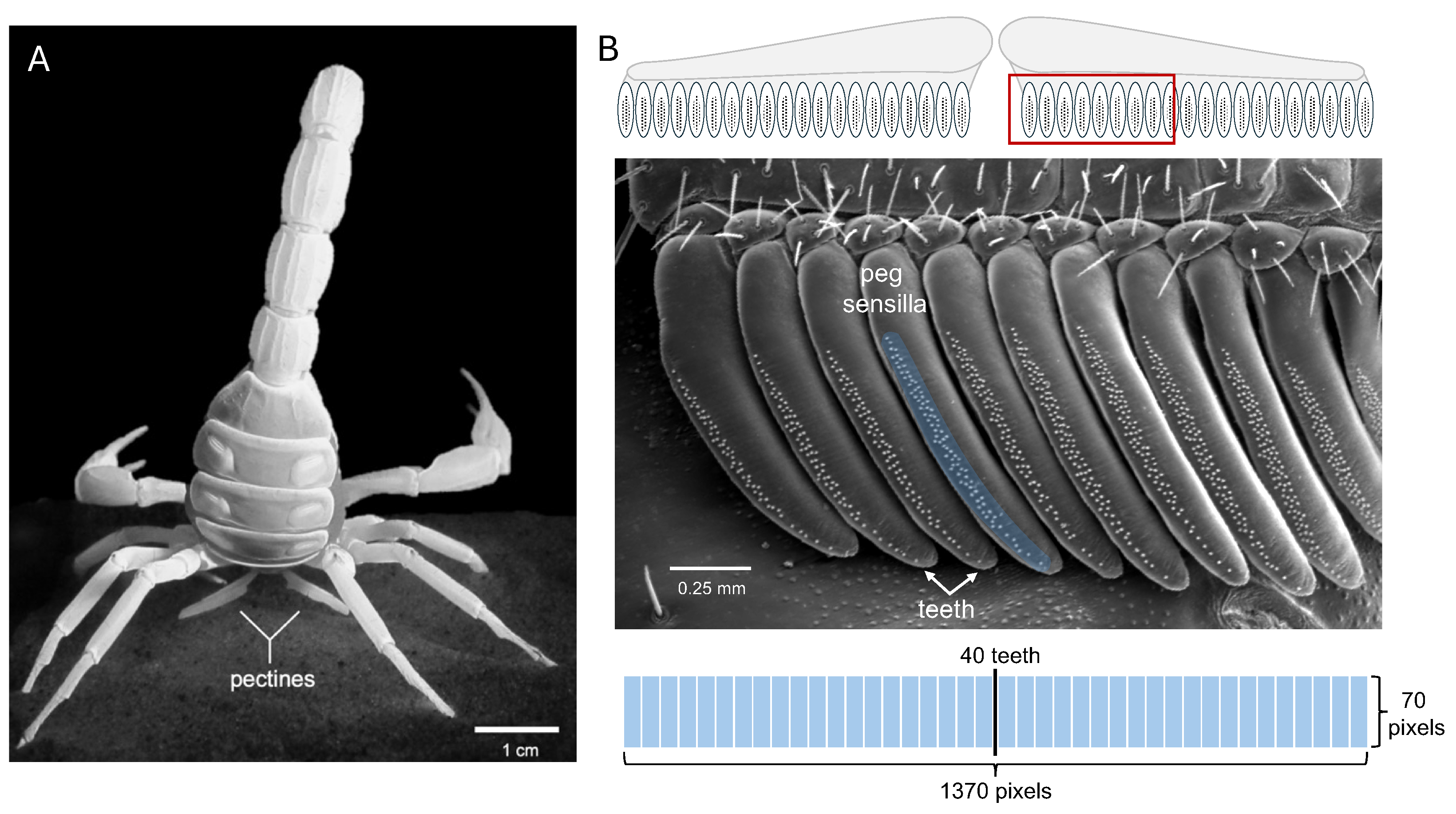
Figure 2.
NFLS memory and processing dynamics. Upper left: a synthetic grayscale landscape with the Initial Journey (IJ, blue) and Subsequent Journey (SJ, purple) overlaid. The agent (scorpion icon; shown half size) first establishes a short, straight IJ path while storing tangent–aligned glimpses in IJ memory (below). During the SJ, at each episode the agent performs a rotational saccade: a local sensor window (simulated pectines, gray rectangle) is rotated through a discrete set of candidate angles (in this case, +35o at 5o increments) around the current pivot location. For each angle, the resulting glimpse is compared to all IJ memories using the sum of absolute differences (SAD). The angle yielding the minimum SAD is selected (in this example, 197 corresponding to IJ index 16) is selected. The agent then steps forward along the best–matching direction, producing a trajectory that converges toward the end of the IJ path using only local familiarity cues. Upper right graph: Minimum SAD as a function of rotation angle, showing a trough at the selected heading. Lower right graph: Minimum SAD as a function of IJ index for the best angle, with the minimum highlighted.
Figure 2.
NFLS memory and processing dynamics. Upper left: a synthetic grayscale landscape with the Initial Journey (IJ, blue) and Subsequent Journey (SJ, purple) overlaid. The agent (scorpion icon; shown half size) first establishes a short, straight IJ path while storing tangent–aligned glimpses in IJ memory (below). During the SJ, at each episode the agent performs a rotational saccade: a local sensor window (simulated pectines, gray rectangle) is rotated through a discrete set of candidate angles (in this case, +35o at 5o increments) around the current pivot location. For each angle, the resulting glimpse is compared to all IJ memories using the sum of absolute differences (SAD). The angle yielding the minimum SAD is selected (in this example, 197 corresponding to IJ index 16) is selected. The agent then steps forward along the best–matching direction, producing a trajectory that converges toward the end of the IJ path using only local familiarity cues. Upper right graph: Minimum SAD as a function of rotation angle, showing a trough at the selected heading. Lower right graph: Minimum SAD as a function of IJ index for the best angle, with the minimum highlighted.
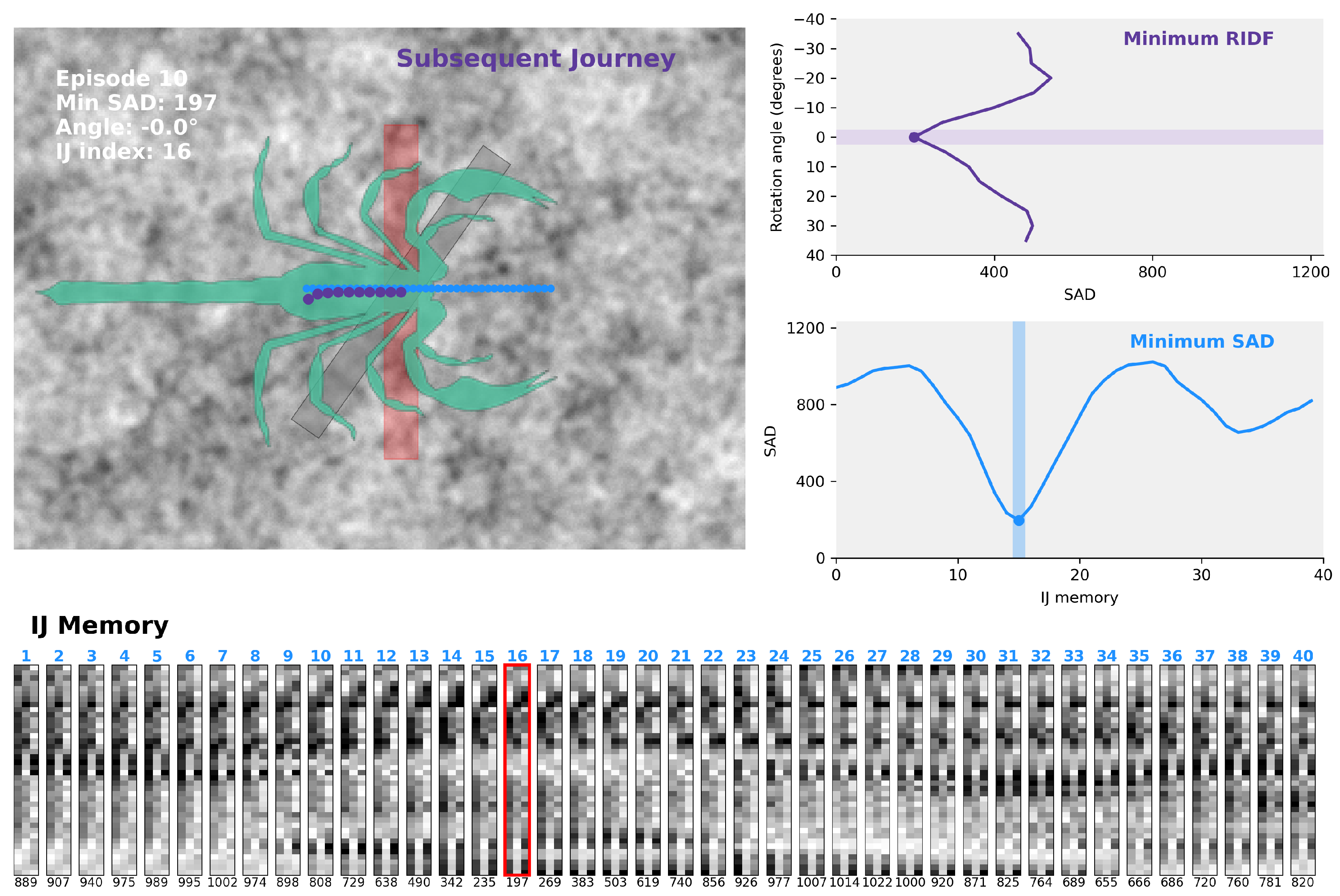
Figure 3.
Robotic car build. Labeled photographs of left side (A) and top (B) of the vehicle. 1) camera, 2) camera support, 3) USB hub, 4) motor driver, 5) left DC geared motor with encoder (one of two) mounted below aluminum plate, 6) wheel (one of two), 7) motor shield, 8) Arduino board, 9) Arduino data cord, 10) Arduino power cord, 11) Raspberry Pi, 12) Pi power port, 13) Pi USB port, 14) clear plastic chassis.
Figure 3.
Robotic car build. Labeled photographs of left side (A) and top (B) of the vehicle. 1) camera, 2) camera support, 3) USB hub, 4) motor driver, 5) left DC geared motor with encoder (one of two) mounted below aluminum plate, 6) wheel (one of two), 7) motor shield, 8) Arduino board, 9) Arduino data cord, 10) Arduino power cord, 11) Raspberry Pi, 12) Pi power port, 13) Pi USB port, 14) clear plastic chassis.
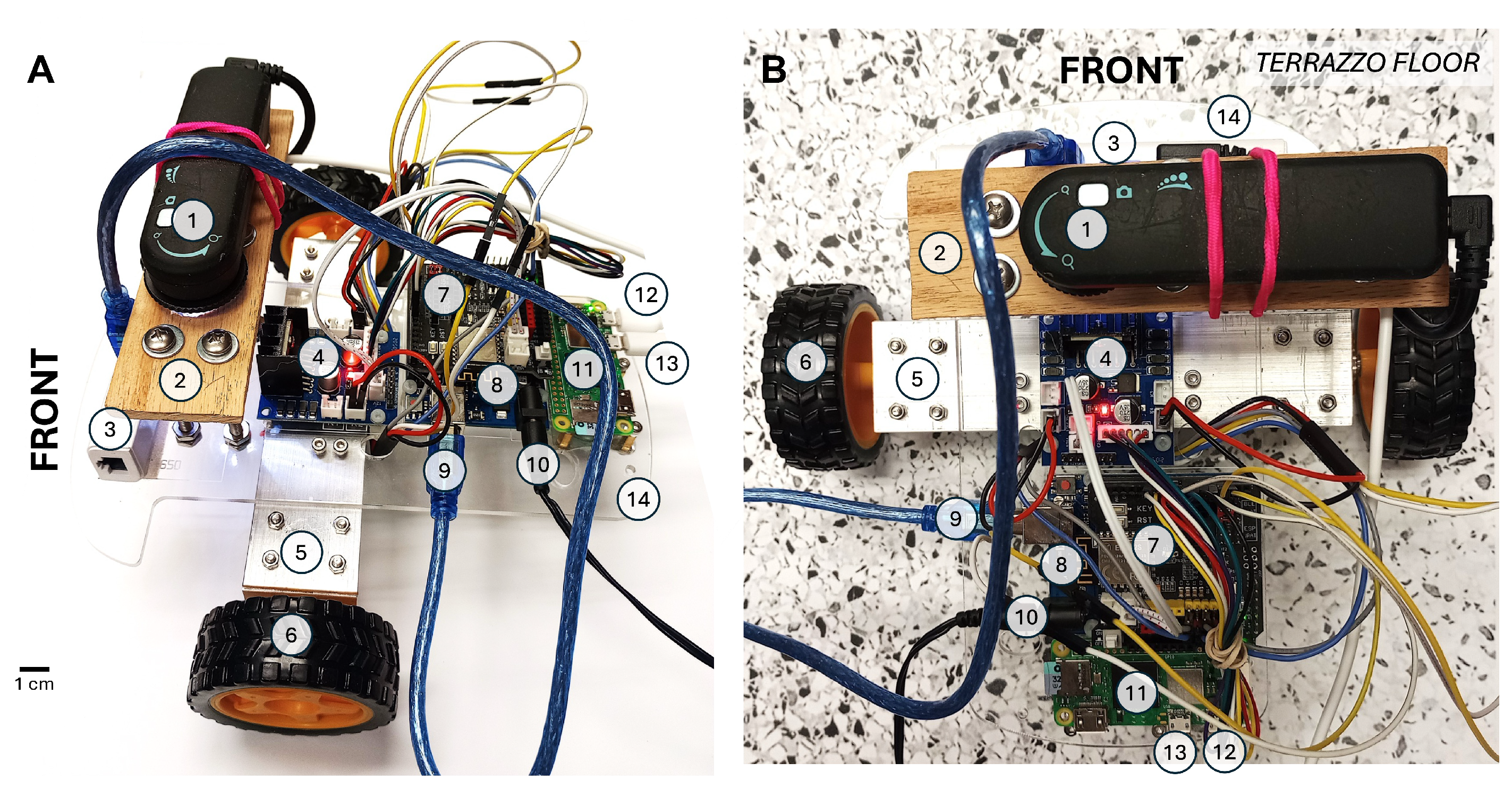
Figure 4.
Scorp-car system architecture. (A) Scorp-car diagram and data flow. The downward-facing camera (C) connects to the USB hub (UH), which connects to the Arduino (Ar) and the Raspberry Pi (Pi).The Arduino connects to the motor shield (MS), which connects to the motor driver (MD), which connects to the left and right DC geared motors (LM, RM), which drive the left and right wheels (LW, RW). The Pi and Arduino are powered by an AC adaptor (AC). RW = rear wheel; OC = OSOYOO chassis. The camera faces downward, is mounted 10.5 cm above the floor, and looks through a rectangular cut in the chassis. (B) Depiction of rotational saccade used in scorp-car (+14o at 2o).
Figure 4.
Scorp-car system architecture. (A) Scorp-car diagram and data flow. The downward-facing camera (C) connects to the USB hub (UH), which connects to the Arduino (Ar) and the Raspberry Pi (Pi).The Arduino connects to the motor shield (MS), which connects to the motor driver (MD), which connects to the left and right DC geared motors (LM, RM), which drive the left and right wheels (LW, RW). The Pi and Arduino are powered by an AC adaptor (AC). RW = rear wheel; OC = OSOYOO chassis. The camera faces downward, is mounted 10.5 cm above the floor, and looks through a rectangular cut in the chassis. (B) Depiction of rotational saccade used in scorp-car (+14o at 2o).
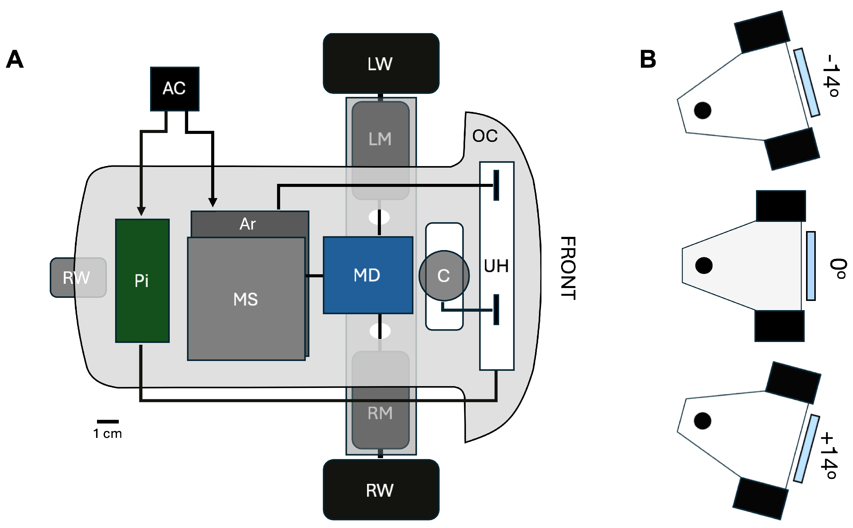
Figure 5.
IJ visualization. Diagram of scorp-car (left) making an IJ over a paper with the letters “T H X” (the letters were 60 mm tall). Visualization of the IJ memory matrix consisting of 40 vertical cells (i.e. teeth) and 60 steps (the glimpse from each step is down-sampled to a 40x1 vector and stored in this matrix). This memory matrix is 2400 bytes or 2.4 kilobytes (i.e., each step requires 40 bytes). The letters are 60 mm tall.
Figure 5.
IJ visualization. Diagram of scorp-car (left) making an IJ over a paper with the letters “T H X” (the letters were 60 mm tall). Visualization of the IJ memory matrix consisting of 40 vertical cells (i.e. teeth) and 60 steps (the glimpse from each step is down-sampled to a 40x1 vector and stored in this matrix). This memory matrix is 2400 bytes or 2.4 kilobytes (i.e., each step requires 40 bytes). The letters are 60 mm tall.
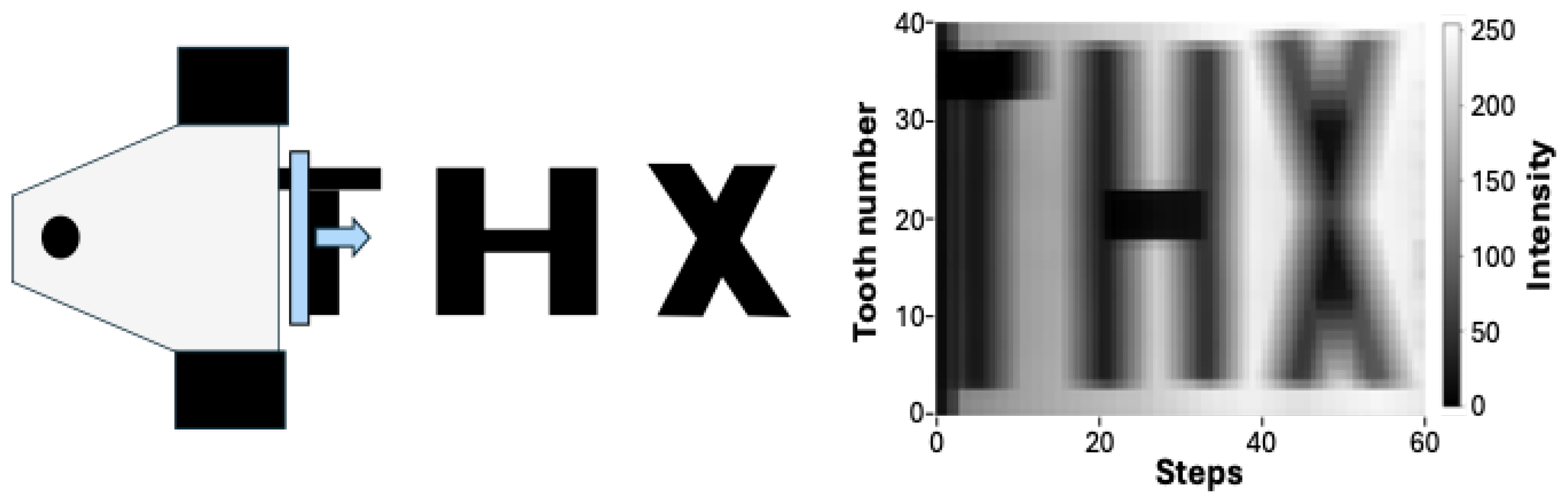
Figure 6.
IJ cross-correlation. (A) Diagram of scorp-car running over a terrazzo landscape. The car captured glimpses during 80 forward steps followed by 80 backward steps. (B) The 160 down-sampled 40-unit vectors are shown as a 40 x 160 matrix. (C) Cross-correlation of the step vectors shows good accuracy of car’s movements.
Figure 6.
IJ cross-correlation. (A) Diagram of scorp-car running over a terrazzo landscape. The car captured glimpses during 80 forward steps followed by 80 backward steps. (B) The 160 down-sampled 40-unit vectors are shown as a 40 x 160 matrix. (C) Cross-correlation of the step vectors shows good accuracy of car’s movements.
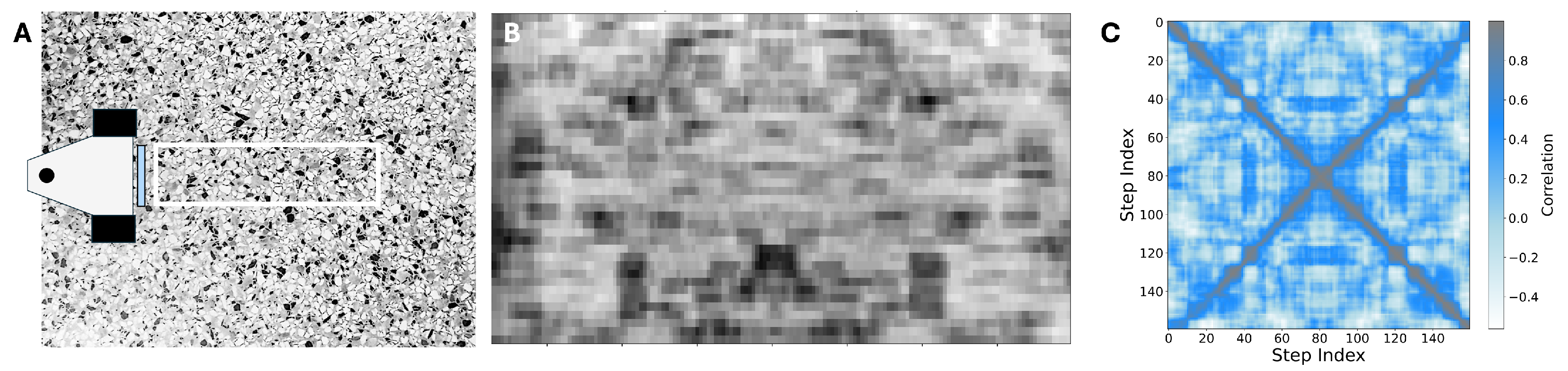
Figure 7.
Catchment troughs. (A) An example of an 80-step IJ across terrazzo landscape (left). The rectangles depict the size of every 10th cropped camera glimpse, and the blue dots indicate the midpoints of all 80 steps and glimpses. SADs were computed using normalized 40-unit down-sampled vectors for each step compared to all other IJ steps. The plot (right) shows the mean SAD + SE for 20 steps before and after each focal step. (B) Depiction of rotational camera glimpses during SJ (left). Only -14o, 0o, and +14o rotations are shown (the scorp-car actually rotates between -14o and +14o at 2o steps for each saccade). The plot (right) shows the mean SAD + SE for the normalized 40-unit vectors of the 15 rotations compared to angle 0o for 20 SJ steps. The dotted lines in the SAD plots of A and B depict 50% of SAD (p50).
Figure 7.
Catchment troughs. (A) An example of an 80-step IJ across terrazzo landscape (left). The rectangles depict the size of every 10th cropped camera glimpse, and the blue dots indicate the midpoints of all 80 steps and glimpses. SADs were computed using normalized 40-unit down-sampled vectors for each step compared to all other IJ steps. The plot (right) shows the mean SAD + SE for 20 steps before and after each focal step. (B) Depiction of rotational camera glimpses during SJ (left). Only -14o, 0o, and +14o rotations are shown (the scorp-car actually rotates between -14o and +14o at 2o steps for each saccade). The plot (right) shows the mean SAD + SE for the normalized 40-unit vectors of the 15 rotations compared to angle 0o for 20 SJ steps. The dotted lines in the SAD plots of A and B depict 50% of SAD (p50).
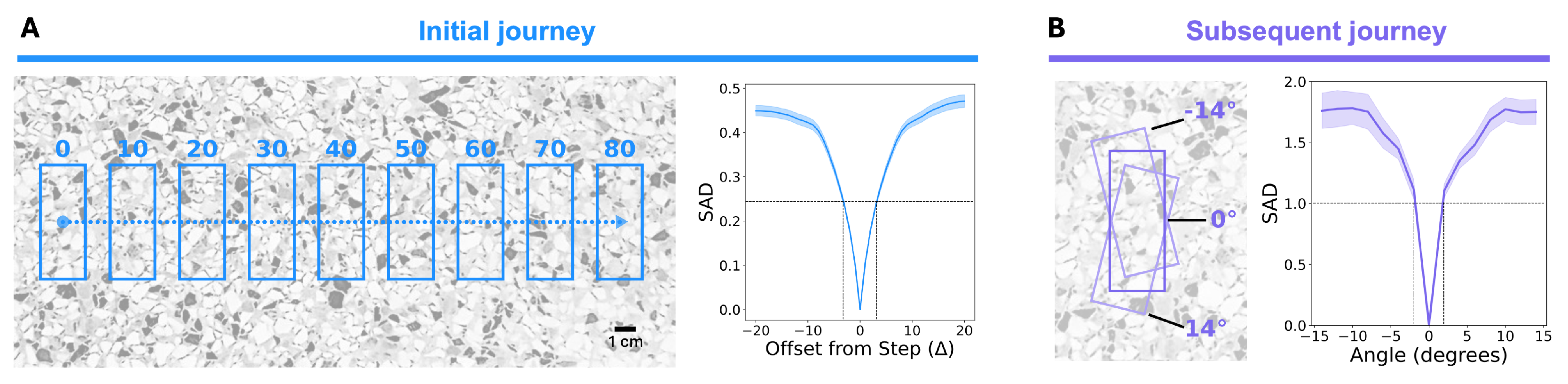
Figure 8.
Potential NFLS catchment information. (A) Superimposed atop a patch of terrazzo landscape are the positions of the 47 IJ steps (blue dots; the path runs from top to bottom). Also superimposed are five equally spaced SJ steps (also running from top to bottom). The orange dots indicate the pivot points of the agent, and the fan-shaped outline indicates the positions of the camera in front of the pivot points and the -14o to +14o rotational saccade. The purple rectangles show the positions of the 15 sampled glimpses at each step; the rectangles are filled with a purple shading that grades from light purple at -14o to dark purple at +14o. [scale bar = 1 cm] (B) The 15 40-unit rotational vectors obtained at each step are stacked and highlighted based on the same color grading used in A (the -14o vector is at top of each block). (C) The minimum SAD of the fifteen rotational vectors compared to the 47 IJ path vectors (D) are plotted and shaded as in A and B. The highlighted rows in B and D indicate the selected SJ rotation angle (B) and the selected IJ path vectors (D) based on minimum overall SAD value at each step.
Figure 8.
Potential NFLS catchment information. (A) Superimposed atop a patch of terrazzo landscape are the positions of the 47 IJ steps (blue dots; the path runs from top to bottom). Also superimposed are five equally spaced SJ steps (also running from top to bottom). The orange dots indicate the pivot points of the agent, and the fan-shaped outline indicates the positions of the camera in front of the pivot points and the -14o to +14o rotational saccade. The purple rectangles show the positions of the 15 sampled glimpses at each step; the rectangles are filled with a purple shading that grades from light purple at -14o to dark purple at +14o. [scale bar = 1 cm] (B) The 15 40-unit rotational vectors obtained at each step are stacked and highlighted based on the same color grading used in A (the -14o vector is at top of each block). (C) The minimum SAD of the fifteen rotational vectors compared to the 47 IJ path vectors (D) are plotted and shaded as in A and B. The highlighted rows in B and D indicate the selected SJ rotation angle (B) and the selected IJ path vectors (D) based on minimum overall SAD value at each step.
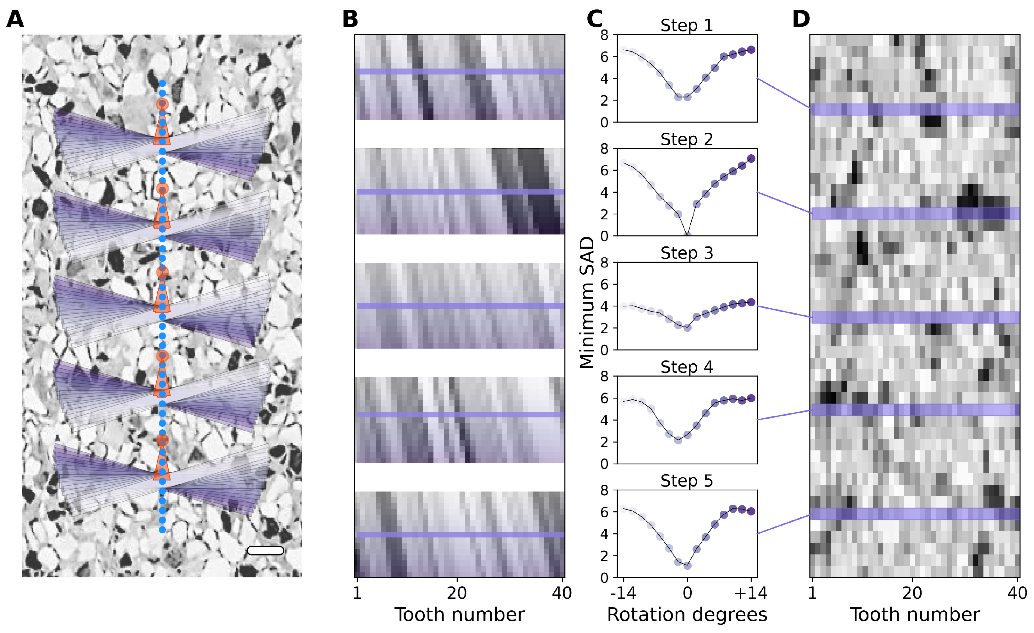
Figure 9.
Scorp-car performance. (A) The patch of terrazzo landscapewith the positions of the 47 IJ steps (blue dots; the path runs from top to bottom; black dashed rectangle depicts the width of the IJ glimpses). [scale bar = 1 cm] (B) The 15 40-unit rotational vectors obtained at each of 15 SJ steps are stacked (the -14o vector is at top of each block). (C) The minimum SAD of the fifteen rotational vectors compared to the 47 IJ path vectors (D) are plotted for the 15 steps. The highlighted rows in B and D indicate the selected SJ rotation angle (B) and the selected IJ path vectors (D) based on minimum overall SAD value at each step. The approximate final SJ path as determined by captured post step glimpses is shown by the purple dots and line in A.
Figure 9.
Scorp-car performance. (A) The patch of terrazzo landscapewith the positions of the 47 IJ steps (blue dots; the path runs from top to bottom; black dashed rectangle depicts the width of the IJ glimpses). [scale bar = 1 cm] (B) The 15 40-unit rotational vectors obtained at each of 15 SJ steps are stacked (the -14o vector is at top of each block). (C) The minimum SAD of the fifteen rotational vectors compared to the 47 IJ path vectors (D) are plotted for the 15 steps. The highlighted rows in B and D indicate the selected SJ rotation angle (B) and the selected IJ path vectors (D) based on minimum overall SAD value at each step. The approximate final SJ path as determined by captured post step glimpses is shown by the purple dots and line in A.
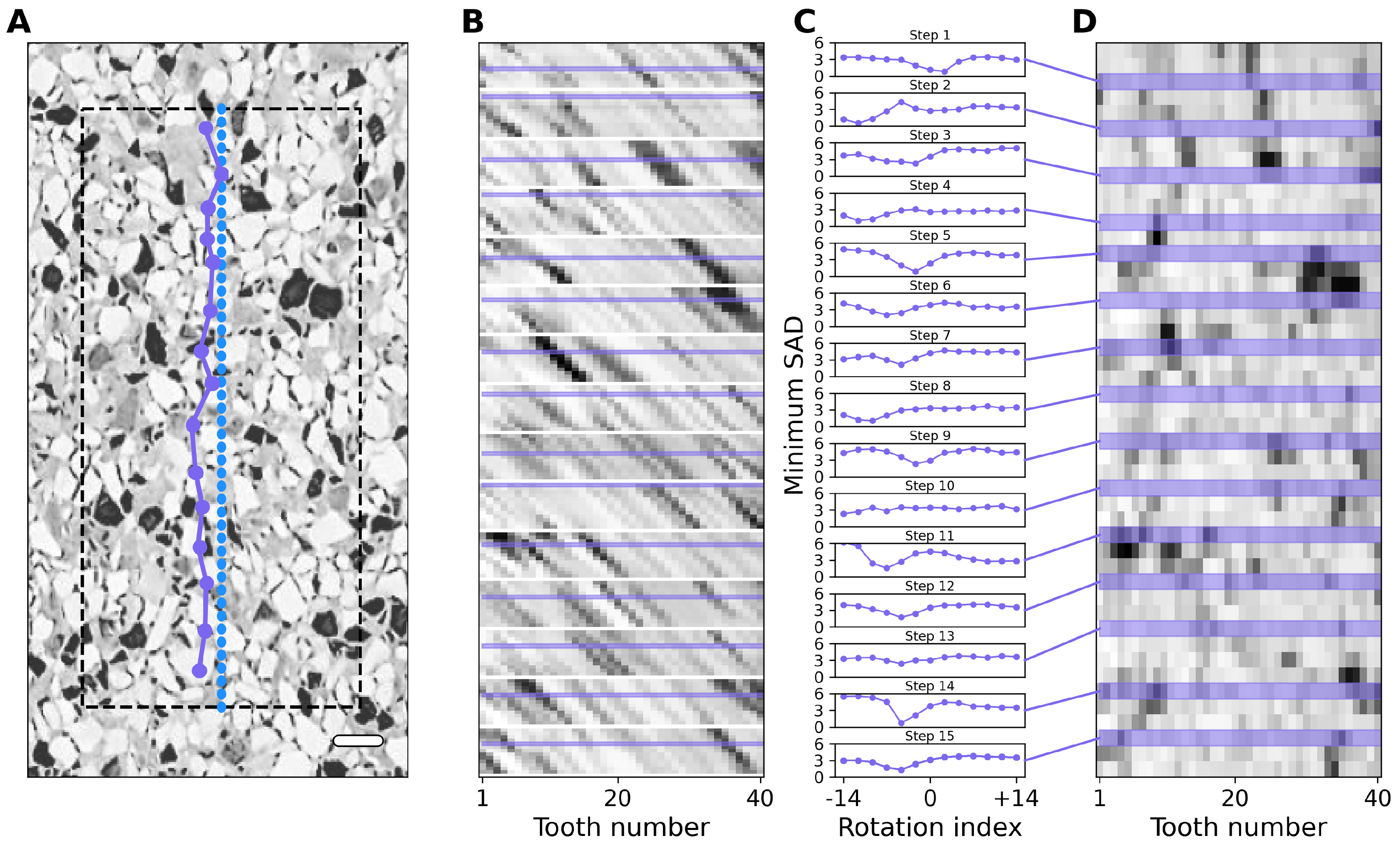
Figure 10.
Scorp-car navigating via NFLS. (A) Screenshots from selected points of the scorp-car’s IJ and SJ movements. (B) Plot of scorp-car SJ positions (purple dots) relative to a curved IJ (blue circles) shows navigational success. [scale bar = 5 cm]
Figure 10.
Scorp-car navigating via NFLS. (A) Screenshots from selected points of the scorp-car’s IJ and SJ movements. (B) Plot of scorp-car SJ positions (purple dots) relative to a curved IJ (blue circles) shows navigational success. [scale bar = 5 cm]
Disclaimer/Publisher’s Note: The statements, opinions and data contained in all publications are solely those of the individual author(s) and contributor(s) and not of MDPI and/or the editor(s). MDPI and/or the editor(s) disclaim responsibility for any injury to people or property resulting from any ideas, methods, instructions or products referred to in the content. |
© 2026 by the author. Licensee MDPI, Basel, Switzerland. This article is an open access article distributed under the terms and conditions of the Creative Commons Attribution (CC BY) license (http://creativecommons.org/licenses/by/4.0/).
Copyright: This open access article is published under a Creative Commons CC BY 4.0 license, which permit the free download, distribution, and reuse, provided that the author and preprint are cited in any reuse.