

Submitted:
28 September 2026
Posted:
30 September 2026
You are already at the latest version
Abstract
Background: Motion during magnetic resonance imaging (MRI) scans is common and can degrade image quality and reduce diagnostic accuracy. This study developed MC-Former, a motion correction method for brain MRI based on vision transformers and self-supervised learning. Methods: Motion-free brain MRI data from 52 subjects were used to generate 13,700 training, 1,950 validation, and 4,680 test axial slices from 3D sagittal T1-weighted scans acquired at 3T. MC-Former was derived from a vision transformer-based encoder-decoder architecture with skip connections. During self-supervised pre-training, 50% of patches from motion-free images were randomly masked and reconstructed; synthetic motion-corrupted images were then used for supervised training. Evaluation was performed on simulated motion-corrupted axial images unseen during training, using peak signal-to-noise ratio (PSNR) and structural similarity index measure (SSIM). Results: MC-Former improved PSNR from 26.4 to 32.8 and SSIM from 0.77 to 0.94, significantly outperforming MC-Net and Restormer on the test set. For motion-free images, MC-Former achieved SSIM > 0.99. Conclusion: These results indicate that MC-Former effectively suppresses simulated motion artifacts in brain MRI while preserving artifact-free image quality. The code and trained model are available at https://github.com/MRIMoCo/MC-Former.
Keywords:
brain MRI
; motion correction
; deep learning
; self-supervised learning
; vision transformer
1. Introduction
Motion during MRI is inevitable and can cause motion artifacts because of the sequential spatial encoding and data acquisition [1,2]. While prospective motion correction techniques can improve MR image quality in the presence of motion [3], post-processing techniques are appealing since they do not require modifications of MR pulse sequences and potential increases in scan times.
Recently, a range of deep learning algorithms have been developed to eliminate motion artifacts from existing brain MRI data [4]. These techniques mostly involve Deep Convolutional Neural Network (DCNN) architectures, including Inception-ResNet [1], variational auto encoders (VAE) [2], and generative adversarial networks (GAN) [5]. In the context of DCNNs, we proposed a novel loss function to improve the performance of a UNet [6] for motion correction in brain MRI [7]. However, CNN-based methods can cause unwanted low-pass filtering and compromise the quality of artifact-free images.
Some of the drawbacks of CNN-based methods may be avoided by the vision Transformer (ViT) [8] and its variants [9,10]. Previous research assessed ViTs in medical image analysis regarding classification, segmentation, lesion or abnormality detection, and medical image restoration [11]. ViTs typically need more training data than CNNs [12,13] and require increased computational capacity due to quadratic complexity of self-attention (SA), but this challenge may be overcome by self-supervised learning (SSL) approaches. SSL commonly uses restorative pre-training formulated as pixel-wise image reconstruction [14], for instance, by masking out portions of an image and teaching a model to in-paint them (“masked image modeling” or MIM) [15]. MIMs also preserve fine-grained textures and are particularly well-suited for ViT pre-training [16,17,18].
Here, we formulate the MRI motion correction problem as an image restoration task and propose a novel method by integrating ViT and SSL to eliminate motion artifacts from brain MRI. We hypothesized that MIM as a restorative pre-training method would improve the performance of a ViT for motion correction [19]. For simplicity, we refer to our hybrid model as a “ViT model” throughout.
2. Materials and Methods
For this retrospective study, approval from the IRB and a waiver for informed consent were obtained. As discussed noted above, MIM may be a suitable pre-processing step for motion correction as it tries to solve a pixel restoration problem which is a low-level vision application as well. We selected a task-specific ViT-based model [20] for high-resolution image restoration as the backbone. We trained and evaluated the ViT using an in-house dataset with simulated motion-artifacts.
2.1. Study Design and Patients
Figure 1 shows the pipeline to generate motion-corrupted data. We started with “clean” images without motion artifacts, based on deidentified brain MRI scans from 52 human subjects (50 male, 2 females, age 48.6 ± 9.1 years) previously enrolled in research studies. All data were acquired with an MPRAGE sequence (T1-weighted with 1mm isotropic resolution) on a 3T scanner (TIM Trio, Siemens Healthcare, Erlangen, Germany). Starting with clean image volumes, motion corruption was performed in k-space by updating the phases according to translations and resampling data according to rotations [21]. Ten axial slices (256×256 array size) spaced 5mm apart were extracted from each “clean” and the corresponding motion-corrupted MPRAGE volume. These images were divided into a training set (35 subjects; 25 motion trajectories; 13,700 slices), a validation set (5 subjects; 7 motion trajectories; 1,950 slices), and a test set (12 subjects; 7 motion trajectories; 4,680 slices). The subjects and motion trajectories in these sets did not overlap.
2.2. Vision Transformer Model
The ViT-model is derived from the Restormer network, which is a task-specific model with an encoder-decoder structure and skip connections [20]. The Restormer is designed for low-level vision problems by designing key building blocks (i.e., multi-head attention and feed-forward network) such that it can capture long-range pixel interactions, while remaining applicable to large images. We optimized our ViT model by using Multi-Depthwise Convolution Head Transposed Attention (MDTA) and Gated-Depthwise Convolutional Feed-Forward Network (GDFN). MDTA [20] was proposed to reduce the complexity of the conventional SA [8] from quadratic to linear by applying SA across channels instead of the spatial dimension as shown in the following:
where X and denote the input and output feature maps. ,
, and are matrices obtained after reshaping the tensor from the original size . are height, width, and channel number. α is a learnable scaling parameter to control the magnitude of the dot product of and . The attention map encoding global context is generated by computing cross-covariance across channels.
Gated-Depthwise Convolutional Feed-Forward Network (GDFN) [20] introduced two improvements based on a conventional feed-forward network. First, the gating mechanism controls the information flow through the respective hierarchical levels, allowing each level to focus on the fine details complementary to the other levels. Second, depth-wise convolutions are used to encode information from spatially neighboring pixel positions and learn local image structure for effective restoration. The GDFN can be expressed as:
where , ⊙, ϕ, and LN denote one input tensor, element-wise multiplication, the GELU non-linearity [22], and layer normalization [23].
2.3. Model Training
As is shown in Figure 2, the ViT model was trained in two stages: SSL pre-training and fully supervised training. We randomly masked 50% of patches of clean input images and predicted the masked patches during pre-training the ViT using MIM. We divided the original images of size 256*256 into non-overlapping patches with an optimized size of 16*16 [16,17], using a batch size of 64. The mean squared error (MSE) loss was used [17].
In the second stage of fully supervised training, we trained the pre-trained model with the AdamW optimizer [24] and L1 loss for 1,200K iterations with an initial learning rate of 3*10-4, which was gradually reduced to 10-6 with cosine annealing. Due to computational limitations, we used a patch of size 128*128 and a batch size of 1 during the second stage. Neighbor patches overlapped by 64 pixels. The model was validated using the peak signal to noise ratio (PSNR) on the validation set during training. When the performance saturated on plateaus, we selected the model with the best PSNR on the validation set as the final model for inference.
After the second stage model training, the test slices with motion artifacts were fed into the final model to predict motion-free images. Additionally, we performed an image quality trustworthiness test, by processing clean images to determine whether a given method injected artifacts. This aspect of performance is important in the clinic, since it is unacceptable for CNNs or ViTs to degrade high-quality input data.
2.4. Quantitative Evaluation Metrics
We quantified the performance of the various methods using two measures: the first is the PSNR, which is the ratio of maximum possible power (MAX) of a signal to the power of distorting noise that affects the quality of its representation (i.e., mean square error between the denoising result from a DL model and the clean reference, MSE):
Second, by using the “clean” image as reference, we calculated the structural similarity index measure (SSIM) [25]:
where x and y denote signals from input and reference, μx, μy, σx, σy, and σxy denote mean of input, mean of reference, variance of input, variance of reference, and covariance, respectively, and C1 and C2 are two constants to prevent the denominator from becoming zero. When the numerical difference between a predicted result and the reference approaches 0, the PSNR approaches infinity and the SSIM approaches 1.
2.5. Statistical Analysis
We compared the MC-Former to the “standard” Restormer model [20] and the MC-Net; the latter is a state-of-the-art CNN based model for brain MRI motion correction [7]. For each method and data set, we calculated the mean value and standard deviation of the SSIM and PSNR. We performed a paired t-test to determine the significance of differences between algorithms, with p<0.05 considered significant. Violin plots were used to illustrate distributions of SSIM and PSNR for all methods for comparison on the in-house dataset.
2.6. Implementation Details
All experiments were conducted on a workstation with a Linux operating system (Ubuntu 20.04; Canonical, London, England), an Intel(R) Xeon(R) Silver 4210R CPU @ 2.40GHz 196GB RAM, and an NVIDIA GeForce RTX 4090 Graphics Cards 24GB. The ViT model was implemented using Pytorch [26] version 2.0.1 with CUDA 12.0 support.
3. Results
3.1. Quantitative Improvements for Motion-Corrupted Images
For motion-corrupted images from the test set, the MC-Former approach achieved an SSIM of 0.94 and a PSNR of 32.8 (Table 1 and Figure 3). These values are significantly better compared with the other two methods (MC-Net and Restormer; paired t-tests p<0.005 for all contrasts). Figure 3 shows the corresponding violin plots of SSIM and PSNR distributions of the raw corrupted images, and the results of the MC-Net, the Restormer, and the MC-Former.
Figure 4 shows representative results for a few slices with severe simulated motion artifacts. The MC-Net, Restormer, as well as the improved image quality, but MC-Former generally recovers more image details than the other two approaches. This is particularly noticeable in the reconstruction of the cerebellar region in Figure 4A and the error maps. Also, the CNN-based approach (MC-Net) shows substantially more blurring (low-pass filtering) than the two vision-transfer based approaches.
3.2. Effect on Motion-Free Images
The effects of processing artifact-free images with the three algorithms is reported in Table 2. For these clean input images, both the Reformer and MC-Former networks showed excellent agreement between their output (corrected) and clean images, with SSIM > 0.99 for both, but the original Reformer method had better average PSNR. Both vision-transfer based approaches achieved better SSIM and PSNR values than MC-Net.
Visually, the ViT approaches (Restormer and the MC-Former) were also better than the MC-Net at retaining image details when “clean” images without motion artifacts were processed (Figure 5). Overall, the output of the Restormer and the MC-Former are visually almost indistinguishable when applied to images without motion artifacts.
3.3. Evaluation of Self-Supervised Pre-Training
Figure 6 compares the progression of PSNR values during supervised ViT model training on the validation set, both with and without MIM pre-training. After approximately 250K iterations, the model with pre-training had higher PSNR values on the validation set. Likewise, the model with pre-training converged and plateaued faster (at around 900K) than the model without pre-training.
3.4. Effect of SSL Patch Size
To optimize the patch size for SSL, we repeated pre-training with different patch sizes of 16*16, 32*32, 64*64, and 128*128, using the same second stage training setup. The mean SSIM for these patch sizes and the test set are shown in Figure 7. Accordingly, the optimal patch size is 16*16 (solid blue line in Figure 7, p < 0.005), although the performance of the model pre-trained with 32*32 is close. We also pre-trained the model with corrupted patches of various sizes (dashed yellow line in Figure 7); again, the patch size of 16*16 is optimal in this case.
4. Discussion
In this work, we considered MRI motion correction as an image-restoration problem and adopted the Restormer and SSL to build a ViT motion correction model named MC-Former. MIM was used to pre-train the MC-Former for pixel restoration as the pre-task. With knowledge transferred from the pre-training, MC-Former is then trained in a fully supervised manner for image restoration. By coupling two highly related tasks (i.e., pixel restoration and image restoration) [19], the MC-Former outperformed the Restormer and MC-Net.
Compared with the UNet-based MC-Net model, the MC-Former was better simultaneously at reducing motion artifacts and preserving fine (high-frequency) details. This is most likely because the “convolution” operation underlying the MC-Net (CNN) focuses on local connectivity and has a limited receptive field, preventing it from modeling long-range pixel dependencies [11]. Conversely, the MC-Former has multiple cascading transformer layers that capture the global context of an input image. The MC-Former generally also outperformed the Restormer [20] designed for high-resolution image restoration. We suggest that the pixel restoration with MIM as the pre-task helps the model learn low-level vision representations.
Compared with the MC-Net, the two vision-transfer based approaches achieved better SSIM and PSNR values and were also better at retaining details of “clean” images (Figure 5). Together, this indicates that ViTs are better able than CNNs to preserve image context.
Unlike conventional supervised learning methods, which are trained on a specific task with a prior based on the available labeled data, SSL learns generic representations across many tasks. SSL is especially useful in medical image analysis where labels are costly and limited, or the specific task cannot be known a priori [27]. By using SSL (i.e., MIM) in our study, we boosted the performance of the ViT without the cost of manual labelling. In addition, the MIM pre-training also resulted in faster convergence for the down-stream task, which is consistent with results from previous studies [28,29,30].
Our study has several limitations. First, the motion artifacts used in this study were synthetically generated. This was necessary to provide motion-free ground-truth images for quantitative evaluation, but the simulated artifacts may not fully capture the complexity and variability of real patient motion during MRI acquisition. Second, all images were acquired from a single scanner and using a single T1-weighted MPRAGE sequence, which may limit the generalizability of the trained model to other scanners, imaging protocols, and patient populations. Third, the model pre-trained with the smallest patch size (16*16) during MIM performed the best on the test set, which is consistent with prior literature [15,31]. Using smaller patches benefits solving dense prediction tasks since the final representations of the learned ViT are more fine-grained [31]. However, we did not assess patch sizes below 16 * 16 because smaller patch sizes result in quadratic increases in computing resources [32]. Additionally, we fixed the mask ratio at 50% and did not try different mask ratios for simplicity. Finally, we did not compare our new method with other CNN-based published methods, mostly since they are not publicly available.
5. Conclusions
To our knowledge, our work is the first to apply ViT-based model for motion correction in brain MRI. By using MIM as the pre-task, the MC-Former generally performed better than the Restormer in terms of PSNR and SSIM and converged faster during ViT training. The MC-Former also reduced motion artifacts better than a CNN-based method (MC-Net), overcame the issue of blurring caused by the CNN model, and simultaneously injected fewer artifacts. Finally, the MC-Former is entirely data-driven and might be integrated into clinical practice.
Author Contributions
Conceptualization, T.E. and Z.W.; methodology, L.Z., X.W. and Z.W.; software, L.Z. and X.W.; validation, L.Z., X.W., L.C., E.H.H. and E.R.M.; formal analysis, L.Z. and X.W.; investigation, Z.W. and T.E.; resources, T.E.; data curation, X.W.; writing—original draft preparation, L.Z.; writing—review and editing, T.E., Z.W., X.W., E.H.H., E.R.M. and L.C.; visualization, L.Z. and X.W.; supervision, T.E. and Z.W.; project administration, T.E.; funding acquisition, T.E. and Z.W. All authors have read and agreed to the published version of the manuscript.
Funding
This research was funded by the National Institutes of Health, grant numbers 1R01DA021146, R01AG060054, R01AG070227, R01EB031080-01A1, R21AG080518, R01AG081693, and P41EB029460-01A1. Lei Zhang was supported in part by start-up funding from the Department of Computer and Information Sciences at Towson University, the Coastal Athletic Association Academic Alliance through the AI Technologies Network Award, the NIH SuRE-First Award, grant number R16EB039671, and Towson University Faculty Development and Research Committee funding.
Institutional Review Board Statement
This retrospective study was approved by the Institutional Review Board, and the requirement for informed consent was waived because the study used de-identified retrospective MRI data.
Informed Consent Statement
Patient consent was waived because this retrospective study used de-identified retrospective MRI data.
Data Availability Statement
Restrictions apply to the datasets used in this study. The datasets are not publicly available because the research participants did not provide explicit consent for data sharing, and the data contain human MRI information subject to privacy and ethical restrictions. Requests for access to the datasets should be directed to Thomas Ernst. The code and trained model are available at https://github.com/MRIMoCo/MC-Former.
Acknowledgments
During the preparation of this manuscript, the authors used ChatGPT for language editing and formatting assistance. The authors have reviewed and edited the output and take full responsibility for the content of this publication.
Conflicts of Interest
The authors declare no conflicts of interest.
References
- Pawar, K.; Chen, Z.; Shah, N.J.; Egan, G.F. Suppressing motion artefacts in MRI using an Inception-ResNet network with motion simulation augmentation. NMR Biomed. 2019, e4225.
- Küstner, T.; Armanious, K.; Yang, J.; Yang, B.; Schick, F.; Gatidis, S. Retrospective correction of motion-affected MR images using deep learning frameworks. Magn. Reson. Med. 2019, 82, 1527–1540.
- Maclaren, J.; Herbst, M.; Speck, O.; Zaitsev, M. Prospective motion correction in brain imaging: A review. Magn. Reson. Med. 2013, 69, 621–636.
- Chang, Y.; Li, Z.; Saju, G.; Mao, H.; Liu, T. Deep learning-based rigid motion correction for magnetic resonance imaging: A survey. Meta-Radiology 2023, 100001.
- Usman, M.; Latif, S.; Asim, M.; Lee, B.D.; Qadir, J. Retrospective motion correction in multishot MRI using generative adversarial network. Sci. Rep. 2020, 10, 1–11.
- Ronneberger, O.; Fischer, P.; Brox, T. U-Net: Convolutional networks for biomedical image segmentation. In Proceedings of the International Conference on Medical Image Computing and Computer-Assisted Intervention, 2015; pp. 234–241.
- Zhang, L.; et al. Motion correction in MRI with large movements using deep learning and a novel hybrid loss function. In Proceedings of ISMRM 2021, 2021.
- Dosovitskiy, A.; et al. An image is worth 16 × 16 words: Transformers for image recognition at scale. 2021. Available online: https://openreview.net/forum?id=YicbFdNTTy.
- Liu, Z.; et al. Swin transformer: Hierarchical vision transformer using shifted windows. In Proceedings of the IEEE/CVF International Conference on Computer Vision, 2021; pp. 10012–10022.
- Guo, M.H.; Liu, Z.N.; Mu, T.J.; Hu, S.M. Beyond self-attention: External attention using two linear layers for visual tasks. IEEE Trans. Pattern Anal. Mach. Intell. 2022, 45, 5436–5447.
- Shamshad, F.; et al. Transformers in medical imaging: A survey. Med. Image Anal. 2023, 102802.
- Tay, Y.; et al. Scaling laws vs. model architectures: How does inductive bias influence scaling? arXiv 2022, arXiv:2207.10551.
- Steiner, A.; Kolesnikov, A.; Zhai, X.; Wightman, R.; Uszkoreit, J.; Beyer, L. How to train your ViT? Data, augmentation, and regularization in vision transformers. arXiv 2021, arXiv:2106.10270.
- Zhou, Z.; Sodha, V.; Pang, J.; Gotway, M.B.; Liang, J. Models Genesis. Med. Image Anal. 2021, 67, 101840.
- Balestriero, R.; et al. A cookbook of self-supervised learning. arXiv 2023, arXiv:2304.12210.
- He, K.; Chen, X.; Xie, S.; Li, Y.; Dollár, P.; Girshick, R. Masked autoencoders are scalable vision learners. In Proceedings of the IEEE/CVF Conference on Computer Vision and Pattern Recognition, 2022; pp. 16000–16009.
- Xiao, J.; Bai, Y.; Yuille, A.; Zhou, Z. Delving into masked autoencoders for multi-label thorax disease classification. In Proceedings of the IEEE/CVF Winter Conference on Applications of Computer Vision, 2023; pp. 3588–3600.
- Xie, Z.; et al. SimMIM: A simple framework for masked image modeling. In Proceedings of the IEEE/CVF Conference on Computer Vision and Pattern Recognition, 2022; pp. 9653–9663.
- Zamir, A.R.; Sax, A.; Shen, W.; Guibas, L.J.; Malik, J.; Savarese, S. Taskonomy: Disentangling task transfer learning. In Proceedings of the IEEE Conference on Computer Vision and Pattern Recognition, 2018; pp. 3712–3722.
- Zamir, S.W.; Arora, A.; Khan, S.; Hayat, M.; Khan, F.S.; Yang, M.H. Restormer: Efficient transformer for high-resolution image restoration. In Proceedings of the IEEE/CVF Conference on Computer Vision and Pattern Recognition, 2022; pp. 5728–5739.
- Zahneisen, B.; Keating, B.; Singh, A.; Herbst, M.; Ernst, T. Reverse retrospective motion correction. Magn. Reson. Med. 2016, 75, 2341–2349.
- Hendrycks, D.; Gimpel, K. Gaussian error linear units. arXiv 2016, arXiv:1606.08415.
- Ba, J.L.; Kiros, J.R.; Hinton, G.E. Layer normalization. arXiv 2016, arXiv:1607.06450.
- Loshchilov, I.; Hutter, F. Decoupled weight decay regularization. arXiv 2017, arXiv:1711.05101.
- Wang, Z.; Bovik, A.C.; Sheikh, H.R.; Simoncelli, E.P. Image quality assessment: From error visibility to structural similarity. IEEE Trans. Image Process. 2004, 13, 600–612.
- Paszke, A.; et al. PyTorch: An imperative style, high-performance deep learning library. Adv. Neural Inf. Process. Syst. 2019, 32.
- Krishnan, R.; Rajpurkar, P.; Topol, E.J. Self-supervised learning in medicine and healthcare. Nat. Biomed. Eng. 2022, 6, 1346–1352.
- Zhang, L.; Mohamed, A.A.; Chai, R.; Guo, Y.; Zheng, B.; Wu, S. Automated deep learning method for whole-breast segmentation in diffusion-weighted breast MRI. J. Magn. Reson. Imaging 2020, 51, 635–643.
- Zhou, Z.; Shin, J.; Zhang, L.; Gurudu, S.; Gotway, M.; Liang, J. Fine-tuning convolutional neural networks for biomedical image analysis: Actively and incrementally. In Proceedings of the IEEE Conference on Computer Vision and Pattern Recognition, 2017; pp. 7340–7351.
- Zhou, S.K.; et al. A review of deep learning in medical imaging: Imaging traits, technology trends, case studies with progress highlights, and future promises. Proc. IEEE 2021, 109, 820–838.
- Yun, S.; Lee, H.; Kim, J.; Shin, J. Patch-level representation learning for self-supervised vision transformers. In Proceedings of the IEEE/CVF Conference on Computer Vision and Pattern Recognition, 2022; pp. 8354–8363.
- Zhang, C.; Zhang, C.; Song, J.; Yi, J.S.K.; Kweon, I.S. A survey on masked autoencoder for visual self-supervised learning. In Proceedings of the Thirty-Second International Joint Conference on Artificial Intelligence, 2023; pp. 6805–6813.
Figure 1.
The two-step pipeline to generate motion-corrupted k-space data. (a) We generated the synthesized motion trajectories in step 1. (b) motion trajectories from step 1 were used to simulate motion artifacts in step 2.
Figure 1.
The two-step pipeline to generate motion-corrupted k-space data. (a) We generated the synthesized motion trajectories in step 1. (b) motion trajectories from step 1 were used to simulate motion artifacts in step 2.
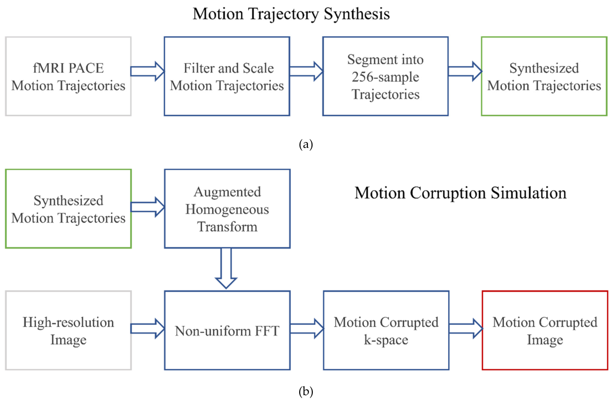
Figure 2.
ViT architecture. During pre-training, half of the clean image patches are masked out, and the ViT is trained to reconstruct the missing patches and hence the original image. After pre-training, the ViT is then trained with much larger patches (with overlap) from corrupted images to reconstruct the clean images.
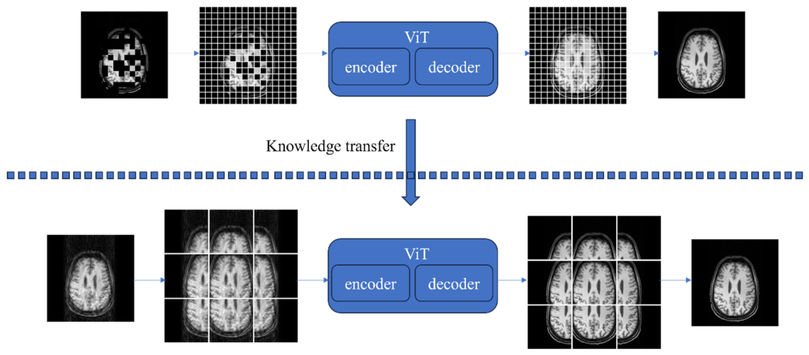
Figure 3.
Violin plot of the (a) structural similarity index measure (SSIM) and (b) peak signal to noise ratio (PSNR) for the corrupted images and those processed with 3 different methods. All contrasts are statistically significant (paired t-test p < 0.005).
Figure 3.
Violin plot of the (a) structural similarity index measure (SSIM) and (b) peak signal to noise ratio (PSNR) for the corrupted images and those processed with 3 different methods. All contrasts are statistically significant (paired t-test p < 0.005).
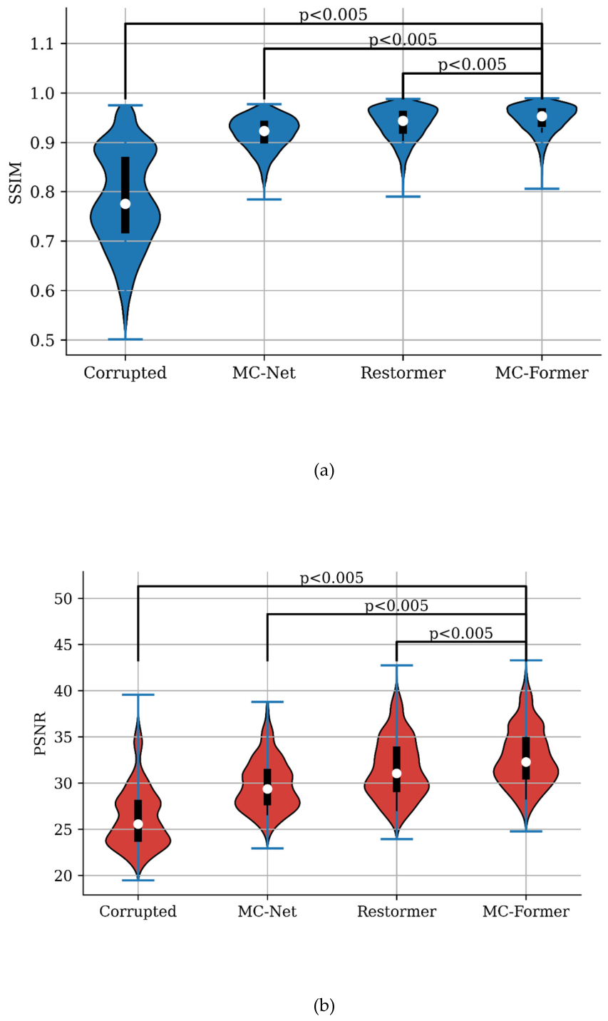
Figure 4.
Examples of motion artifact removal from images in the test data set using MC-Net, Restormer, and the MC-Former. In Figure 4A,B, the first row of each subfigure contains the “clean” (reference) image, corrupted image, and motion correction results using the three algorithms. The SSIM and PSNR values for each corrected image (relative to the “clean” image) are also shown. The second row of each subfigure zooms in on the red rectangle. The third row shows the error maps between reference image (i.e., clean image) / motion corrupted image and motion correction results, using the absolute value of the difference between results and clean reference multiplied by a factor of five.
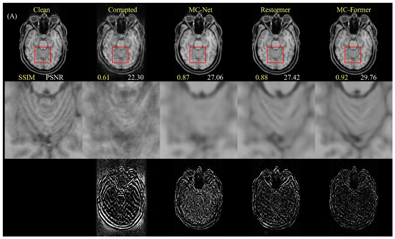
Figure 5.
Examples of processing clean images in the test data set using various algorithms. In Figure 5A,B, the first row of each subfigure contains the clean reference image and motion correction results using the MC-Net, Restormer, and the MC-Former. The SSIM and PSNR values for each corrected image (relative to the “clean” image) are also shown. The second row of each subfigure zooms in on the red rectangle. The third row shows the error maps between reference image (i.e., clean image) / motion corrupted image and motion correction results, using the absolute value of the difference between results and clean reference multiplied by a factor of ten.
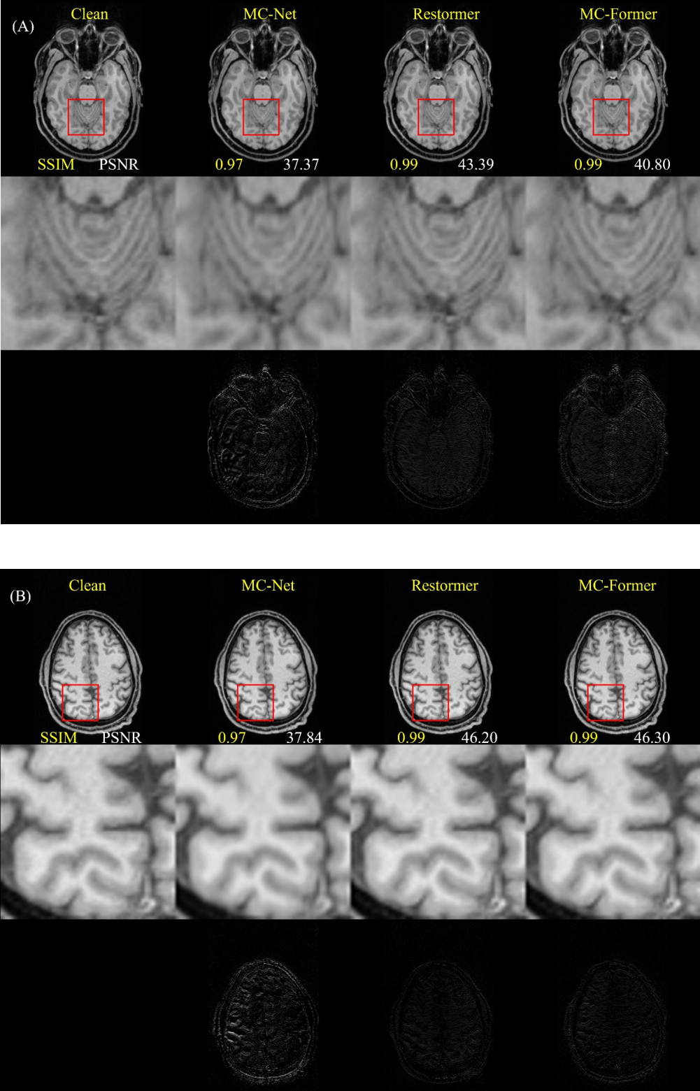
Figure 6.
PSNR curves on validation set during ViT model supervised training (with MIM pre-training versus without MIM pre-training).
Figure 6.
PSNR curves on validation set during ViT model supervised training (with MIM pre-training versus without MIM pre-training).
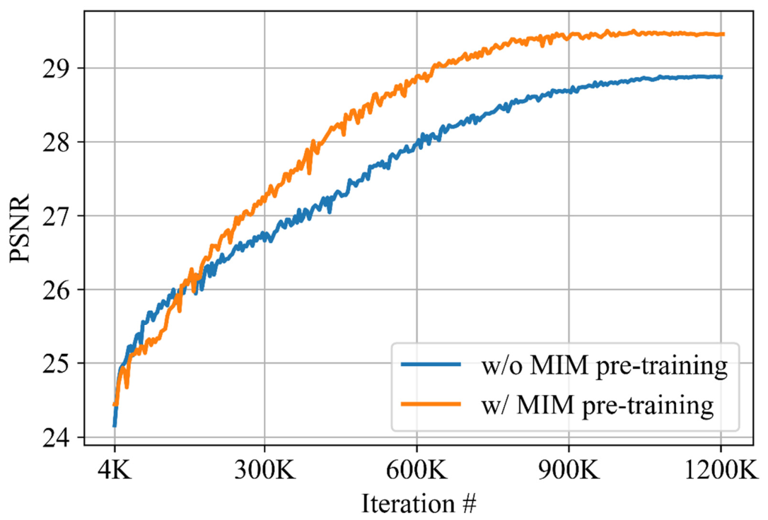
Figure 7.
SSIM scores of models pre-trained using SSL with different patch sizes. The x-axis represents the patch size, and the y-axis shows mean SSIM scores of images from the test set of the in-house dataset. Error bars represent standard errors of the mean SSIM scores.
Figure 7.
SSIM scores of models pre-trained using SSL with different patch sizes. The x-axis represents the patch size, and the y-axis shows mean SSIM scores of images from the test set of the in-house dataset. Error bars represent standard errors of the mean SSIM scores.
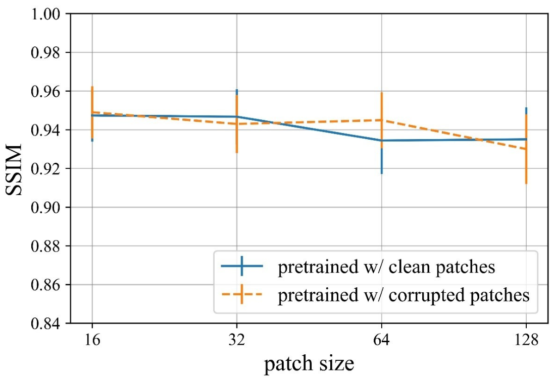

Table 1.
Results of applying motion-removal networks to motion-corrupted images from the test set. The table lists the SSIM (mean ± SD) and PSNR (mean ± SD) of corrupted and corrected images processed using the MC-Net, Restormer, and the MC-Former.
Table 1.
Results of applying motion-removal networks to motion-corrupted images from the test set. The table lists the SSIM (mean ± SD) and PSNR (mean ± SD) of corrupted and corrected images processed using the MC-Net, Restormer, and the MC-Former.
| Corrupted | MC-Net | Restormer | MC-Former | |
| SSIM | 0.77 ± 0.099 | 0.92±0.033 | 0.93±0.033 | 0.94±0.029 |
| PSNR | 26.4 ± 3.3 | 29.8 ± 2.7 | 31.5± 3.3 | 32.8±3.2 |
Table 2.
Results of applying motion-removal networks to motion-free images from the test set. The table lists the SSIM (mean ± SD) and PSNR (mean ± SD) of images after applying the MC-Net, Restormer, and the MC-Former.
Table 2.
Results of applying motion-removal networks to motion-free images from the test set. The table lists the SSIM (mean ± SD) and PSNR (mean ± SD) of images after applying the MC-Net, Restormer, and the MC-Former.
| Corrupted | MC-Net | Restormer | MC-Former | |
| SSIM | 0.77 ± 0.099 | 0.92±0.033 | 0.93±0.033 | 0.94±0.029 |
| PSNR | 26.4 ± 3.3 | 29.8 ± 2.7 | 31.5± 3.3 | 32.8±3.2 |
Disclaimer/Publisher’s Note: The statements, opinions and data contained in all publications are solely those of the individual author(s) and contributor(s) and not of MDPI and/or the editor(s). MDPI and/or the editor(s) disclaim responsibility for any injury to people or property resulting from any ideas, methods, instructions or products referred to in the content. |
© 2026 by the authors. Licensee MDPI, Basel, Switzerland. This article is an open access article distributed under the terms and conditions of the Creative Commons Attribution (CC BY) license (http://creativecommons.org/licenses/by/4.0/).
Copyright: This open access article is published under a Creative Commons CC BY 4.0 license, which permit the free download, distribution, and reuse, provided that the author and preprint are cited in any reuse.