
Submitted:
28 September 2026
Posted:
29 September 2026
You are already at the latest version
Abstract
In this work, we develop a differential-geometric framework for superpolar geometries, extending the superelliptic structures introduced in previous studies to manifold structures generated by Gielis’ general superformula. A superpolar Riemannian structure is introduced through a compatible metric induced by the general superformula, and the resulting manifold structure and associated geometric properties are investigated. Within this framework, we construct superpolar lines, planes, and spheres and study various superpolar submanifolds, including conic submanifolds, spheres, rectifying submanifolds, and rectifying hypersurfaces. A fundamental feature of this framework is that curves and surfaces which, from the Euclidean viewpoint, may appear as squares, triangles, symmetric or asymmetric shapes, or even irregular forms with sharp points and corners, can be regarded intrinsically as circles and spheres with respect to the superpolar metric. In other words, structures that appear irregular or anisotropic in Euclidean geometry may correspond to regular geometric objects in their intrinsic geometry. Thus, the observed anisotropy is not an intrinsic property of the geometry, but rather a consequence of its Euclidean embedding.
Keywords:
superpolar geometry
; Gielis superformula
; superpolar manifold
; superpolar submanifolds
1. Introduction
If mathematics is truly to become the language of nature, also of the living, it might retrace the steps taken by Kepler, Galileo and Newton, beginning with a generalization of the conic sections—a program initiated by Gabriel Lamé in 1818 [1]. Lamé introduced supercircles (more generally superellipses) defined by the equation
of which the classical ellipses, circles, squares, and diamonds arise as the special cases. Originally intended to model the shape of crystals [1], superellipses have recently been found in many natural forms and phenomena [2,3,4,5,6,7]. It allows modeling, for example, tree rings of softwoods in two numbers only. Direct quantification of area through integration is straigthforward, but recently, also methods for computing the perimeter have been found [8,9].
The Gielis superformula [10] constitutes a still broader generalization of the conic sections: it extends Lamé’s superellipses to arbitrary rotational symmetries by allowing independent exponents and a symmetry parameter m, generating supershapes. In the natural sciences, this superformula has proved a remarkably versatile model for a wide range of biological forms. It is a generic geometric continuous transformation between both abstract and natural forms, their development and evolution.
Inspired by this, the notions of a superelliptic inner product [11,12] and of a star derivative [13] have been introduced. The superelliptic product allowed to define orthogonality adapted to the shape. For example, two arms of a starfish, spaced apart, are orthogonal in the superelliptic sense, and this extends to any two adjacent radii in regular polygons. The star derivative allowed for the computation of the curvature in a superelliptic sense. As an immediate consequence, every superelliptic circle possesses constant superelliptic curvature. In this precise sense, all supershapes are reduced to circles. The apparent anisotropy of the shapes in Figure 1 and Figure 2 arises solely from their Euclidean embedding, but intrinsically they are circles and spheres, respectively. In addition, irregularities—regions of vanishing or infinite classical curvature—are absorbed into the underlying metric. The stretchable radius has constant length everywhere, so that the curves (and surfaces) generated by the superformula are simultaneously unit circles and totally osculating shapes [14]. The same geometric framework yields a natural link with quaternion algebras. By reinterpreting rotation in the superelliptic setting one recovers, for example, the classical logarithmic spiral as a circle also when the spiral is modified by the superformula [15].
The star derivative itself may be viewed as the composition of the ordinary differential operator with a radial scaling function; the separation of variables is therefore built into the calculus from the outset. The resulting differential geometry provides a coherent description of curvature, singularities, and geometric structures, and opens the way to a unified treatment of higher-dimensional analogs of the classical theory of curves and surfaces.
In the present paper, we show how both constructions extend to general manifolds. Although earlier work concentrated on the Gielis formula, the superelliptic inner product and the star derivative admit far wider application: any sufficiently smooth and periodic function can serve as the radial function. Because the adjective “superelliptic” has become too restrictive, we henceforth adopt the term superpolar. The term “polar” emphasizes that one begins from a distinguished center, and “superpolar” then allows this position vector to stretch according to a well-defined intrinsic or prescribed geometry.
In this article, we first construct the superpolar geometry itself, with examples of superpolar lines, planes, and spheres. Then we examine manifolds equipped with this structure, the associated Riemann tensor fields, and the geometry of superpolar submanifolds. In the final section, examples of conic submanifolds and spheres, rectifying submanifolds, and rectifying hypersurfaces are provided.
2. Foundations of Superpolar Geometry
Let
We define the superpolar inner product
by
where for .
Particular instances of are superellipses, the superformula and the general superformula [16]
where are continuous functions; are real numbers, with . The standard Gielis Superformula [10] is obtained for , moderating the function . If, in addition, and , Lamé’s superellipses result. The denominator 4 is strictly unnecessary, since the same results can be simply obtained by changing the values and , but it is used to preserve the connection to the original form of the Gielis Superformula and the special case of Lamé curves for , in a rectangular coordinate system.
To ensure the metric coefficient is well-defined and non-degenerate, we require and assume that the parameters and functions are chosen such that the trigonometric terms do not vanish simultaneously, thereby avoiding any singularities:
Since and , the bilinear form is symmetric and positive definite:
To show that the bilinear form determines a valid Riemannian metric, we need to prove that it is symmetric, bilinear, and positive definite on .
- 1.
-
Bilinearity: Let and let . By definition, we have:Due to the linearity of the summation and scalar multiplication, linearity in the second argument is proven analogously. Thus, is bilinear.
- 2.
-
Symmetry: For any , since standard multiplication in is commutative (), we obtain:Therefore, is a symmetric form.
- 3.
-
Positive Definiteness: For any , consider the evaluation of with itself:Since and the trigonometric terms do not vanish simultaneously (), the radius function satisfies , which implies that . Furthermore, given that for all and , every term in the sum is non-negative.Thus, , and equality holds if and only if for all (i.e., ). Consequently, is positive definite.
Hence, it determines a Riemannian metric on . The resulting metric space is called the n-dimensional superpolar space and is denoted by
The metric tensor associated with is
and
The induced norm is given by
Two vectors are said to be superpolar orthogonal if
Let be the standard basis of . The corresponding superpolar orthonormal basis
is defined by
It follows immediately that
Therefore, every vector
admits the representation;
This metric construction furnishes a natural geometric setting in which classical Euclidean geometry is generalized through a superpolar deformation governed by the parameters and . It is defined as the superpolar cross product of two vectors in , given by
where
Determining the cosine of the angle between two non-zero superpolar vectors and is given by
Consequently, the angular parameterization of a superellipse or a superellipsoid can be obtained through the parameter , which serves as the intrinsic angular coordinate induced by the superpolar metric structure. In particular, the parameter generalizes the classical Euclidean polar and spherical angular variables, allowing the geometry of superpolar manifolds to be expressed in a smooth parametric form compatible with the underlying inner product structure. This formulation preserves the geometric interpretation of angles while extending the classical trigonometric framework to the superpolar setting [12].
The superpolar hypersphere of radius R and center is the subset
The following figures illustrate a sequence of superpolar circles and spheres obtained from the standard Gielis superformula. Figure 1 and Figure 2 illustrate the superpolar circles and spheres generated using different parameter sets of the standard Gielis Superformula. It can be observed that when the resulting superpolar circle and spheres is identical to the classical Euclidean circle and sphere, respectively.
Let be a fixed point and let be a non-zero direction vector. The superpolar line passing through in the direction of is defined as the set
Here, t is a real parameter, and the expression is called the superpolar parametric equation of the line with superpolar direction .
Figure 3 illustrates the superpolar lines generated using different parameter sets of the Gielis Superformula. It can be observed that when the resulting superpolar line is identical to the classical Euclidean straight line.
The set
is defined as superpolar hyperplane that is superpolar orthogonal to and passes through .
Figure 4 illustrates the superpolar planes generated using different parameter sets of the Gielis Superformula. It can be observed that when the resulting superpolar plane is identical to the classical Euclidean plane.
For each point , the superpolar tangent space at p is denoted by
A superpolar smooth vector field on is a smooth map
satisfying
The set of all smooth vector fields on is denoted by
With respect to the orthonormal frame
every vector field
can be uniquely represented as
where , then we have
are smooth functions.
Definition 1
(Component Representation Operator). Let
be a fixed ordered basis of . Define the linear operator
by
Since the basis E is fixed, the vectors are regarded constants; consequently, differentiation acts only on the scalar coordinate functions.
Definition 2
(Star Derivative). Let be open and let
where is a fixed basis. Thestar derivativeof f is defined componentwise by
or equivalently,
Equivalently,
Definition 3
(Star Gradient). Let be an open set and let
be differentiable. Let
be a fixed ordered basis of . Thestar gradientof f is defined by
that is,
The framework of superpolar geometry provides a systematic mathematical approach for analyzing figures characterized by irregularities, sharp corners, asymmetry, and other non-smooth geometric features. This framework is particularly useful for extending conventional geometric analysis to shapes that cannot be adequately represented by standard smooth curves or regular geometric structures. As example of continuous functions , Figure 1 and Figure 2 present superpolar circles generated using the standard Gielis superformula, providing classical examples characterized by regularity, symmetry, and smoothly varying radial structures. In the same sense, the graphs in Figure 3 and Figure 4 are lines and planes in the superpolar sense. In contrast, Figure 5 and Figure 6 present geometries generated using the generalized formulation. The resulting geometries exhibit a gradual transition from regular and symmetric configurations to increasingly irregular, asymmetric, and highly spiked forms. They can all be considered as circles and spheres within the superpolar framework.

Table 1.
Parameters used for the cases illustrated in Figure 5.
Table 1.
Parameters used for the cases illustrated in Figure 5.
| Case | c | d | ||||||||||
|---|---|---|---|---|---|---|---|---|---|---|---|---|
| (a) | 30 | 30 | 3 | 3 | 2 | 7 | 1 | |||||
| (b) | 30 | 30 | 3 | 3 | 2 | 7 | 1 | |||||
| (c) | 30 | 30 | 3 | 3 | 2 | 7 | 1 | |||||
| (d) | 30 | 30 | 31 | 3 | 3 | 2 | 7 | 1 | ||||
| (e) | 30 | 30 | 5 | 3 | 3 | 2 | 7 | 1 |
3. Superpolar Manifolds
In this section, we present a framework for manifolds constructed within the setting of superpolar geometry.
A superpolar Riemannian metric on superpolar manifold M is defined as a mapping for . Here, denotes the superpolar tangent space, and represents the superpolar dual space of . The mapping is said to be a superpolar Riemannian metric if, for all , the following conditions hold:
Under these conditions, the pair is called a superpolar Riemannian manifold.
Let , then, for , the star directional derivative on a superellitic Riemannian manifold is defined as follows:
Example 1.
Consider the scalar-valued function and . The superpolar gradient of the function is
Thus the star directional derivative computed as
The superpolar Lie bracket is defined by
then the superpolar Lie bracket of the superpolar vector fields X and Y can be written explicitly as
Moreover, the superpolar Lie bracket on the superpolar manifold is defined for a differentiable function f and vector fields by
With this bracket operation, the space acquires the structure of an infinite-dimensional Lie algebra over . In particular, the Lie bracket satisfies the superpolar Jacobi identity:
for all . Furthermore, may be regarded as a module over the ring of smooth functions on M. Specifically, for and , the vector field is defined pointwise by
With this module structure, the superpolar Lie bracket satisfies the following compatibility relation:
for all and . A superpolar Lie algebra over is a real vector space together with a bilinear map
called the superpolar Lie bracket, satisfying the following axioms for all :
- 1.
- Skew-symmetry:
- 2.
- Jacobi identity:
The superpolar connection is a map
The superpolar covariant derivative of the vector field with respect to is defined as follows:
Example 2.
Consider the vector fields
defined on . The directional derivative of the vector field Y along the vector field X is defined by
Definition 4.
The mapping , defined on the superpolar manifold M is called a superpolar metric tensor if it satisfies the following conditions for each :
- 1.
- for all ,
- 2.
- for all ,
- 3.
- is a bilinear mapping,
where denotes the superpolar tangent space of the superpolar manifold M. Moreover, the following relation holds for the components of the superpolar metric tensor:
where represent the components of the superpolar metric tensor. Since is bilinear, it can be represented by a superpolar matrix, whose inverse is denoted by .
Definition 5.
Let denote the superpolar covariant derivative on the superpolar manifold . The operator is called a superpolar affine connection if it satisfies the following properties:
- 1.
- ,
- 2.
- ,
- 3.
- ,
- 4.
- ,
where , , and f is a superpolar differentiable function.
Proposition 1.
Let denote the superpolar affine connection on the superpolar manifold . Then
- (1)
- ,
- (2)
- ,
where and is the inverse matrix of .
Proof.
Statement (1) is an immediate consequence of properties given in Definition 5. To prove (2), let us put in the superpolar Koszul formula characterized by
Since the brackets are zero, it leaves
But from the definition of Christoffel symbols we have
Attacking both equations with yields the required formula. □
Definition 6.
The components of the superpolar affine connection on the superpolar Riemannian manifold are given by
Here, are called to as the superpolar Christoffel symbols. Moreover, if , the expression can be rewritten as:
In particular, if one selects and , then the following relation holds:
Theorem 1.
Let be a superpolar affine connection on the superpolar Riemannian manifold . Then, for , the following expression holds:
Proof. Let and . The superpolar covariant derivative of the superpolar vector field Y in the direction of X is computed as follows:
Theorem 2.
The superpolar affine connection on the superpolar manifold is symmetric if and only if .
Proof. Let
Taking Equation (12) into account, this expression can be rewritten as
Suppose that the superpolar affine connection is symmetric, that is, . Then we obtain
From this, it immediately follows that
Conversely, if we assume , then we arrive at
4. Superpolar Riemann Tensor Fields
Definition 7.
Let be a superpolar affine connection on the superpolar manifold . The mapping , defined for by
is called the superpolar torsion of , or the superpolar torsion tensor field.
Theorem 3.
Let be a superpolar tensor field on the superpolar manifold . Then satisfies the following properties:
- 1.
- ,
- 2.
- .
Proof.
From the definition of the superpolar torsion tensor field given in Equation (20), we obtain
This establishes the first assertion of the theorem. For the second part, by using the defining properties of the superpolar affine connection given in Definition 5 together with Equation (12), we obtain
Moreover, by invoking the first part of the theorem, we derive
□
Definition 8.
Let be a superpolar affine connection on the superpolar manifold . If , then is said to be torsion-free (or symmetric), and the following identity holds:
The unique torsion-free connection compatible with is called the superpolar Levi–Civita connection and is characterized by:
and satisfies
Definition 9.
Let be a superpolar affine connection on the superpolar manifold . If the following condition is satisfied, namely , then is said to be compatible with the metric . For , this condition is expressed as
Definition 10.
Let be a superpolar affine connection on the superpolar manifold . If is both symmetric and compatible with , then it is called the superpolar Levi-Civita connection, or equivalently, the superpolar Riemannian connection.
Example 3.
Consider a two-dimensional superpolar manifold with the parametrization φ, where and ϕ represents a superpolar angle:
We now determine the components of the superpolar metric tensor and the associated superpolar Christoffel symbols . The superpolar partial derivatives of φ with respect to R and ϕ are computed as follows:
Hence, the components of the superpolar metric tensor are obtained as
Since is symmetric, we also have . Accordingly, the superpolar matrix corresponding to the components of is given by
Furthermore, the superpolar determinant of this matrix is computed as follows:
Therefore, the inverse of the superpolar matrix is obtained as
We now compute the superpolar Christoffel symbols using the metric coefficients:
In a similar manner, one obtains
We now compute the values of the superpolar Levi-Civita connection with respect to the superpolar basis vectors:
where and .
Definition 11.
Let be the superpolar Levi-Civita connection on the superpolar manifold . The superpolar curvature tensor is defined as the mapping for all by
Here, denotes the superpolar Riemannian connection on the superpolar Riemann manifold , and it defines a mapping for all . In addition, the components are defined by choosing , , and as
Theorem 4.
The superpolar Riemann curvature tensor of the superpolar manifold has the following component expression:
Proof.
Using Equation (17), we compute
Since , this reduces to
Expanding the covariant derivatives, we obtain
Substituting and yields
Collecting coefficients of completes the derivation.
□
Definition 12.
A superpolar manifold is said to be superpolar flat if , where denotes the superpolar Riemann curvature tensor of the manifold.
Theorem 5.
The superpolar Euclidean space is a superpolar flat manifold; that is, its superpolar Riemann curvature tensor satisfies .
Proof.
The superpolar Euclidean space is equipped with a constant superpolar Euclidean metric, which is invariant at every point of the space. Considering Equation (16), we have
where . Since the components of the superpolar Euclidean metric are constant in the superpolar sense, their corresponding superpolar derivatives vanish, i.e., 0. Therefore, from Equation (16), we obtain
Substituting this result into Equation (22), it follows immediately that
□
5. Superpolar Submanifolds
Let be a superpolar Riemannian manifold, and let denote the superpolar tangent space of M at a point p. Furthermore, suppose that is a superpolar differentiable mapping of class up to order k. The superpolar differential of F at the point is defined as the linear map
where .
The mapping F is called a superpolar immersion whenever the differential is injective for every point . Moreover, if the metric is preserved under the differential, namely,
then the superpolar immersion F is referred to as a superpolar isometric immersion.
It follows immediately that can be regarded as a subspace of . Consequently, the ambient superpolar tangent space admits the following superpolar orthogonal decomposition:
where denotes the superpolar normal space of M at p, and its elements are referred to as superpolar normal vectors to M.
Let
be a mapping satisfying . Such an assignment is called an r-dimensional superpolar distribution. The distribution D is said to be superpolar differentiable of class provided that, for every , there exist r superpolar linearly independent vector fields of class spanning . We denote by the collection of allsuperpolar sections of the distribution D. Furthermore, D is called superpolar involutive if
for every , where denotes the superpolar Lie bracket.
Let M be a superpolar submanifold of . M is called an superpolar integral manifold of D when for every . If there is no other superpolar submanifold containing M, then it is said to be maximal. If in addition there is a maximal superpolar integral manifold of for every , then D is called superpolar integrable.
The following theorem establishes the superpolar extension of the classical Frobenius theorem.
Theorem 6.(superpolar Frobenius theorem). Let D be a superpolar involutive distribution on . Then, for each , there exists a unique maximal superpolar integral manifold M associated with . Furthermore, every superpolar integral manifold passing through q is an open superpolar submanifold of M.
Proof.
Let X and Y be superpolar tangent vector fields on M, and let and denote arbitrary extensions of these vector fields to the ambient space . The covariant derivative of along admits the following superpolar orthogonal decomposition:
where and denote the superpolar tangential and superpolar normal components of with respect to M, respectively. Equation (23) is referred to as the superpolar Gauss formula, while the tensor is called the superpolar second fundamental form. In particular, the submanifold M is said to be superpolar totally geodesic whenever vanishes identically. □
Proposition 2.
Let be a superpolar immersion of the superpolar Riemannian manifold into . Then the following statements hold:
- 1.
- defines a superpolar Riemannian connection on M.
- 2.
- h is a superpolar bilinear and symmetric tensor.
Proof.
Fix an arbitrary point . Around the image point , extend all vector fields and functions defined on M to a neighborhood in . Let X, U, and V be superpolar tangent vector fields on M, where X is chosen arbitrarily, and denote their corresponding extensions by , , and .
1. By means of the superpolar Koszul formula, define
Let . Restricting to M yields
together with
Consequently,
Since X is tangent to M, the decomposition given by the superpolar Gauss formula implies
because the second fundamental form is superpolar normal to M. Therefore, satisfies the defining properties of a superpolar Riemannian connection.
2. The superpolar bilinearity of h follows immediately from its definition. To establish symmetry, observe that
Hence, h is symmetric. □
Let be a superpolar orthonormal basis of . The superpolar mean curvature is defined by
We call Msuperpolar minimal if and superpolar totally umbilical if
for every superpolar tangent to M.
Example 4.
In the three-dimensional superpolar space , the superpolar sphere illustrated in Figure 6 is an example of a totally umbilical surface. Indeed, for every tangent vector fields , the second fundamental form satisfies
Thus, the principal curvatures of the superpolar sphere are equal at every point, and hence superpolar sphere is totally umbilical.
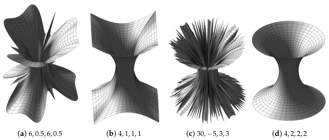
On the other hand, the catenoid shown in Figure 7 is an example of a superpolar minimal surface in . Its mean curvature vanishes identically, that is,
Therefore, the superpolar catenoid
is a superpolar minimal surface.
The superpolar first normal space at in is a superpolar subspace of the superpolar normal space defined by
where is used in the superpolar sense.
Let be a superpolar normal vector field along M in . The covariant derivative of with respect to a superpolar tangent vector field admits the unique superpolar orthogonal decomposition
where and denote the superpolar tangential and superpolar normal components of relative to M, respectively. Equation (27) is referred to as the superpolar Weingarten formula, while the operator A is called the superpolar shape operator.
Proposition 3.
Let be a superpolar immersion of the superpolar Riemannian manifold into , and let ξ be a superpolar normal vector field along M. Then the following assertions hold:
- 1.
- The superpolar shape operator is superpolar linear and satisfiesfor every superpolar tangent vector fields X, Y and every superpolar normal vector field ξ along M.
- 2.
- defines a superpolar natura connection satisfyingfor every superpolar tangent vector field X and every pair of superpolar normal vector fields ξ, η along M.
Proof.
- 1.
-
Let and let . By the linearity of the ambient superpolar Riemannian connection,where denotes the superpolar Riemannian connection on . Applying the superpolar Weingarten formula (27) and comparing the superpolar tangential components, we obtainwhich proves the superpolar linearity of the shape operator.To establish the stated identity, let Y be a superpolar tangent vector field and let be a superpolar normal vector field along M. Since , differentiation along yields
- 2.
- The proof follows the same argument as in the first part. Replacing the tangent vector field Y by a superpolar normal vector field and applying the superpolar Weingarten formula immediately givesthereby proving that is a superpolar natural connection.
□
5.1. Superpolar Conic Submanifolds and Spheres
A superpolar cone in with vertex q is defined as a superpolar submanifold formed by a family of superpolar lines emanating from the point q. A local parametrization of such a superpolar cone is given by
where is a local coordinate chart of an -dimensional superpolar Riemannian manifold. An superpolar conic submanifold of with vertex q is defined to be any open subset of a superpolar cone having vertex q, where is constant.
A superpolar submanifold of is called superpolar spherical if it is contained in a superpolar hypersphere of .
A nonzero vector field is said to be superpolar concurrent provided that
As an illustration, consider the radial vector field and let
Then,
which shows that the radial vector field is a superpolar concurrent vector field. Let be a superpolar isometric immersion. For every point , denote by and the superpolar orthogonal projections onto and , respectively. Then, we write as follows:
In what follows, we characterize superpolar submanifods in in terms of the superpolar tangential and superpolar normal components of their position vectors.
Proposition 4.
Let be a superpolar isometric immersion. Then
- 1.
- if and only if M is a superpolar conic submanifold with vertex at 0.
- 2.
- if and only if M is contained in a superpolar spherical manifold centered at 0.
Proof.
- 1.
-
Assume first that for every . Defineso that and . Sincetaking the superpolar derivative with respect to yieldswhere denotes the superpolar Riemannian connection on . Furthermore, since F is superpolar concurrent, we haveOn the other hand,Since the left-hand side is equal to and is superpolar orthogonal to , it follows immediately thatTherefore, the superpolar integral curves of are superpolar geodesics in . Moreover, because F is the position vector field and , these geodesics pass through the origin. Consequently, M is a superpolar conic submanifold with vertex at 0.Conversely, suppose that M is a superpolar conic submanifold with vertex at 0. Then M admits the given parametrization:From this parametrization, it is evident that is superpolar parallel to one of the basis vectors of the superpolar tangent space. Hence,This establishes the first assertion.
- 2.
-
Assume thatFor every and every , we haveSinceandit follows thatHence, is constant on M. Therefore, M is contained in a superpolar hypersphere of centered at the origin.Conversely, if M is contained in a superpolar hypersphere centered at 0, then the position vector field is everywhere superpolar normal to M, which immediately impliesThis completes the proof.
□
5.2. Superpolar Rectifying Submanifolds
In this section, we introduce the notion of superpolar rectifying submanifolds.
Definition 13.
Let be a superpolar immersion of a superpolar Riemannian manifold into . The submanifold M is called an superpolar rectifying submanifold of if
Furthermore, if
then M is called a proper superpolar rectifying submanifold.
Remark 1.
Let M be a proper superpolar rectifying submanifold of dimension n in . Then
The above inequality follows by contradiction. Suppose that
Observe that the inequality
cannot occur since
for every . Consequently,
Since
it follows that
Hence,
which implies
This contradicts the assumption that M is proper, thereby completing the proof.
Theorem 7.
Let be a superpolar isometric immersion of a superpolar Riemannian manifold into with . Then M is a proper superpolar rectifying submanifold if and only if is a superpolar concurrent vector field on M. The converse is also true.
Proof.
Let and denote the superpolar Riemannian connection on and the induced superpolar Riemannian connection on M, respectively. Let . Since F is a concurrent vector field, we have
Applying the superpolar Gauss and superpolar Weingarten formulas yields
Comparing the superpolar tangent components of both sides, we obtain
Assume first that M is a proper superpolar rectifying submanifold. By Definition 13, for every ,
Therefore, by the first assertion of Proposition 3,
This immediately gives
showing that is a superpolar concurrent vector field on M.
Conversely, suppose that
Then we obtain
By the first assertion of Proposition 3, it follows that
Since is tangent to M, we also have
Consequently,
which, by Definition 13, shows that M is a proper superpolar rectifying submanifold. This completes the proof. □
5.3. Superpolar Rectifying Hypersurfaces
We begin by characterizing the superpolar totally geodesic submanifolds of .
Proposition 5.
A superpolar n-dimensional superpolar totally geodesic submanifold of is an open subset of a superpolar linear subspace of . Conversely, every open subset of a superpolar linear subspace is a superpolar totally geodesic submanifold.
Proof.
Let be a superpolar immersion of an n-dimensional superpolar totally geodesic submanifold. Since M is superpolar totally geodesic, its second fundamental form vanishes identically. Therefore, the superpolar Gauss formula reduces to
Hence, every superpolar geodesic of M is also a superpolar geodesic of , and conversely. Suppose that M contains a point p satisfying
Then is a superpolar linear subspace of . Since the superpolar geodesics of are precisely the superpolar straight lines, it follows that M is an open subset of the superpolar linear subspace whose superpolar tangent space at the origin is .
The converse follows immediately, since every superpolar linear subspace has vanishing second fundamental form and is therefore superpolar totally geodesic. □
Now let M be a superpolar hypersurface of with superpolar unit normal vector field Z. Assume further that M is a superpolar rectifying submanifold. In this case, the superpolar first normal space at each point is the superpolar line spanned by Z, and the defining condition in Definition 13 becomes
Since
and
for some smooth function on M, we obtain
Therefore, a superpolar rectifying hypersurface cannot be proper when its dimension is .
The following theorem provides a complete classification of superpolar rectifying hypersurfaces in .
Theorem 8.
Let be a superpolar immersion of an -dimensional superpolar Riemannian manifold into . Then M is a superpolar rectifying hypersurface if and only if it is an open subset of a superpolar hyperplane.
Proof.
Let be arbitrary. From the previous discussion,
Hence,
and since the position vector field is superpolar concurrent in , we have
Applying the superpolar Gauss formula (23), we obtain
Since
the shape operator satisfies
by the first assertion of Proposition 3. Consequently, M is superpolar totally geodesic. The desired conclusion now follows directly from Proposition 5. □
6. Conclusions
This paper extends earlier results [11,12,13,14] in a Riemannian framework. By replacing the Euclidean metric with a superpolar metric, a broad class of natural and abstract geometric objects can be investigated within a unified intrinsic setting. In particular, all Gielis curves, including non-smooth and polygonal shapes, are interpreted as superpolar circles with respect to the proposed metric. Consequently, geometric objects that are extrinsically distinct in Euclidean space become intrinsically equivalent in superpolar geometry.
This intrinsic equivalence considerably simplifies the mathematical treatment of manifolds and submanifolds. Objects such as superpolar spheres with sharp corners or polygonal boundaries possess the same intrinsic geometric structure as the classical Euclidean sphere under the proposed metric. Therefore, many differential geometric constructions can be extended beyond the smooth Euclidean setting without introducing additional analytical complexity. The proposed framework thus provides a natural generalization of manifold and submanifold theory while preserving the essential geometric properties of the underlying space.
Another important consequence of this approach is the reinterpretation of singularities. Features that are regarded as geometric singularities from the Euclidean viewpoint, such as corners or non-smooth boundaries, need not represent intrinsic singularities in superpolar geometry. Instead, they arise as artifacts of the Euclidean metric rather than of the geometric object itself. This observation offers a new perspective on the notion of regularity and suggests that geometric singularities should be understood relative to the metric structure under consideration.
Overall, the proposed superpolar geometry establishes an alternative geometric paradigm in which shape is determined by intrinsic metric properties rather than by Euclidean appearance. From this perspective, geometrically different objects may share an identical intrinsic structure, allowing polygonal and smooth geometries to be studied within the same differential geometric framework. It is expected that this viewpoint will stimulate further developments in differential geometry and find applications in all of the natural sciences, certain human sciences, and in various fields of technology.
References
- Lamé, G. Examen des différentes méthodes employées pour résoudre les problèmes de géométrie; Mme.Ve. Courcier: Paris, 1818. [Google Scholar]
- Shi, P. J., Huang, J. G., Hui, C., Grissino-Mayer, H. D., Tardif, J. C., Zhai, L. H., ... & Li, B. L. (2015). Capturing spiral radial growth of conifers using the superellipse to model tree-ring geometric shape. Frontiers in Plant Science, 6, 856. [CrossRef]
- Huang, W.; Li, Y.; Niklas, K. J.; Gielis, J.; Ding, Y.; Cao, L.; Shi, P. A superellipse with deformation and its application in describing the cross-sectional shapes of a square bamboo. Symmetry 2020, 12(12), 2073. [Google Scholar] [CrossRef]
- Li, Y.; Niklas, K. J.; Gielis, J.; Niinemets, Ü.; Schrader, J.; Wang, R.; Shi, P. An elliptical blade is not a true ellipse, but a superellipse – Evidence from two Michelia species. J. For. Res. 2022, 33(4), 1341–1348. [Google Scholar] [CrossRef]
- Huang, W.; Ma, K.; Gladish, D. K. Ellipse or superellipse for tree-ring geometries? evidence from six conifer species. Trees 2024, 38(6), 1403–1413. [Google Scholar] [CrossRef]
- Li, Q., Niklas, K. J., Niinemets, Ü., Zhang, L., Yu, K., Gielis, J., ... & Shi, P. (2024). Stomatal shape described by a superellipse in four Magnoliaceae species. Botany Letters,171(1), 93-101. [CrossRef]
- Shi, P.; Liu, X.; Gielis, J.; Beirinckx, B.; Niklas, K. J. Comparing six nonlinear equations describing the 2-D profiles of apical meristems. Am. J. Bot. 2026, 113(4), e70177. [Google Scholar] [CrossRef]
- K. C. Suggestion of a Perimeter Formula for Super Ellipses and Their Use in Rectangular Boundary Value Problems in Physics. Karaelmas Sci. Eng. J. 2022, 12, 166–176. [CrossRef]
- Rodriguez, R. O.; Montilla, Y. Hypergeometric Series Representations for the Perimeter of Lamé Superellipses. arXiv 2026, arXiv:2607.09048. [Google Scholar]
- Gielis, J. A Generic Geometric Transformation that Unifies a Wide Range of Natural and Abstract Shapes. Am. J. Bot. 2003, 90, 333–338. [Google Scholar] [CrossRef]
- Özdemir, Z.; Parlak, E. Superquadric Motion and Superquadric Hyperbolic Split Quaternion Algebra Via Gielis Formula. Math. Methods Appl. Sci. 2025. [Google Scholar] [CrossRef]
- Parlak, E.; Özdemir, Z. Superelliptic quaternions and superelliptic rotations with applications. Physica Scr. 2025, 100(9), 095212. [Google Scholar]
- Özdemir, Z.; Parlak, E.; Gielis, J. A unified superelliptic framework for the differential geometry of Gielis transformations. Axioms 2026, 15(5), 1–36. [Google Scholar] [CrossRef]
- Gielis, J.; Özdemir, Z.; Caratelli, D. Unit circles and osculating curves. Reports of Enlarged Sessions of the Seminar of I. Vekua Institute of Applied Mathematics Volume 2026, Volume 40. [Google Scholar]
- Özdemir, Z.; Gielis, J. Metric-induced rotations with Gielis Formula. Mathematics 2026, 14(15), 2828. [Google Scholar] [CrossRef]
- Gielis, J.; Natalini, P.; Ricci, P. E. A note about generalized forms of the Gielis formula. In Modeling in Mathematics: Proceedings of the Second Tbilisi-Salerno Workshop on Modeling in Mathematics; Atlantis Press: Paris, April 2017; pp. 107–116. [Google Scholar]
Figure 1.
Superpolar circles generated using the standard Gielis Superformula (Equation (3)) for different parameter sets . The parameter values are indicated below each subfigure.
Figure 1.
Superpolar circles generated using the standard Gielis Superformula (Equation (3)) for different parameter sets . The parameter values are indicated below each subfigure.
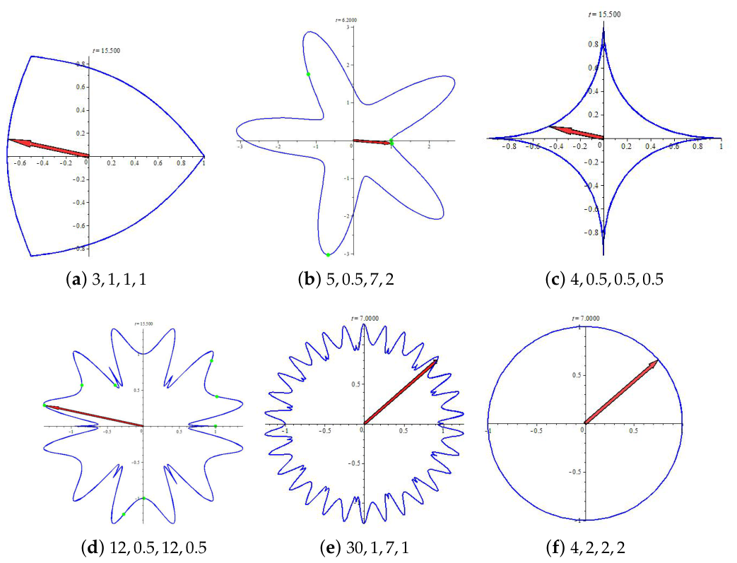
Figure 2.
Superpolar spheres generated using the standard Gielis Superformula (Equation (3)) for different parameter sets . The parameter values are indicated below each subfigure.
Figure 2.
Superpolar spheres generated using the standard Gielis Superformula (Equation (3)) for different parameter sets . The parameter values are indicated below each subfigure.
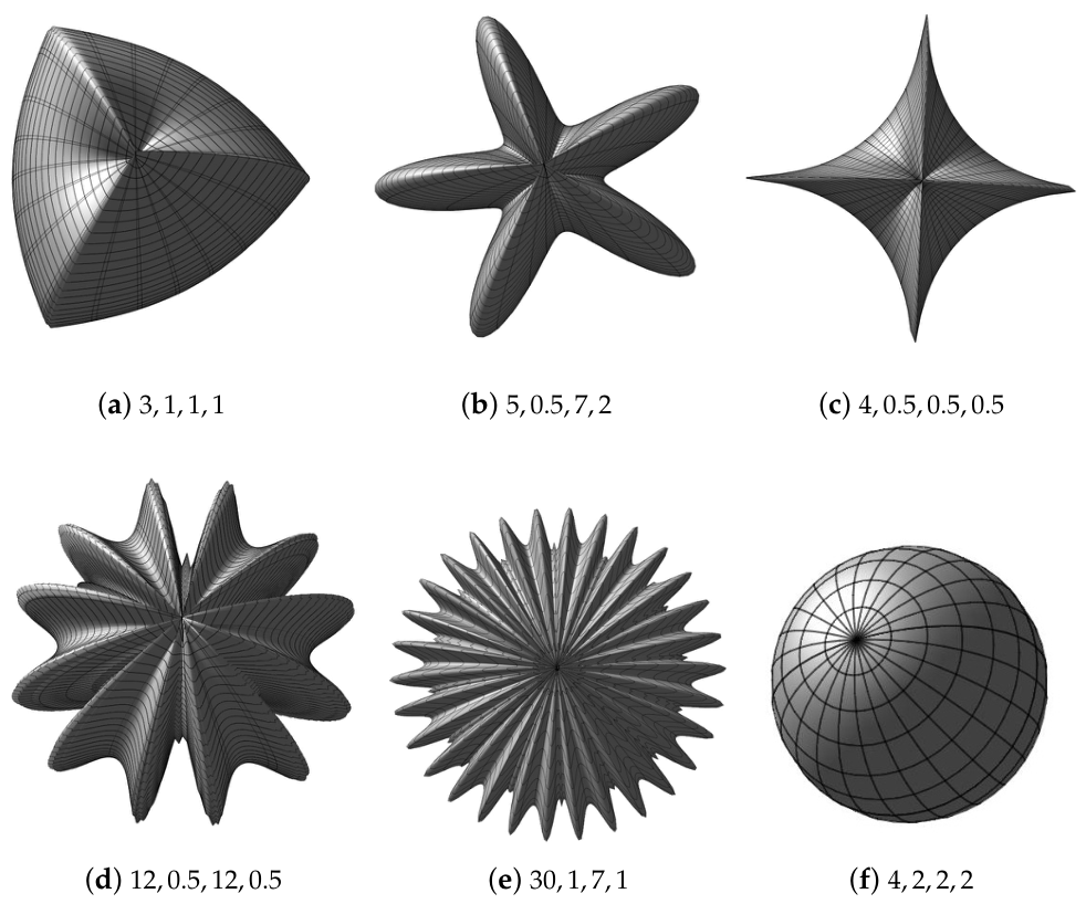
Figure 3.
Superpolar lines generated using the Gielis Superformula (Equation (3)) for different parameter sets . The parameter values are indicated below each subfigure.
Figure 3.
Superpolar lines generated using the Gielis Superformula (Equation (3)) for different parameter sets . The parameter values are indicated below each subfigure.
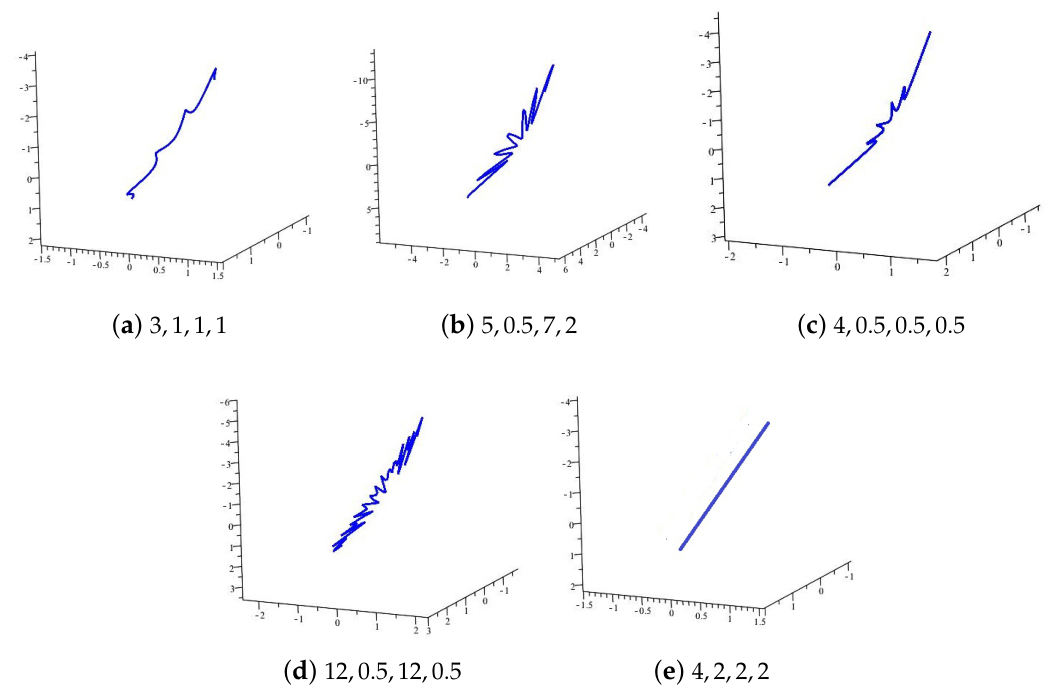
Figure 4.
Superpolar planes generated using the Gielis Superformula (Equation (3)) for different parameter sets . The parameter values are indicated below each subfigure.
Figure 4.
Superpolar planes generated using the Gielis Superformula (Equation (3)) for different parameter sets . The parameter values are indicated below each subfigure.
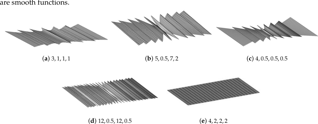
Figure 5.
Superpolar circles generated using the Gielis Superformula (Equation (3)) for different parameter sets in Table 1, for .
Figure 5.
Superpolar circles generated using the Gielis Superformula (Equation (3)) for different parameter sets in Table 1, for .
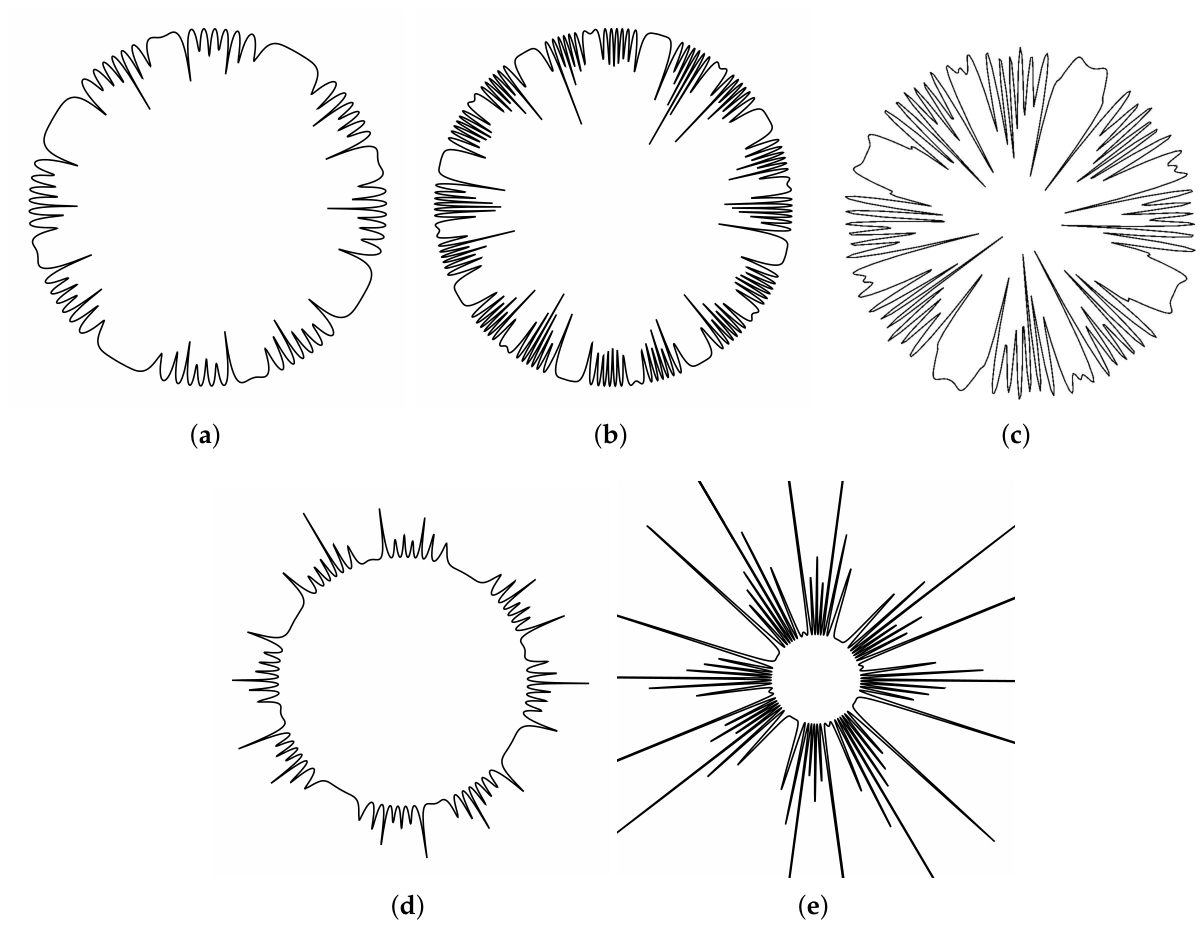
Figure 6.
Superpolar spheres generated using the Gielis Superformula (Equation (3)) for different parameter sets in Table 1, for .
Figure 6.
Superpolar spheres generated using the Gielis Superformula (Equation (3)) for different parameter sets in Table 1, for .
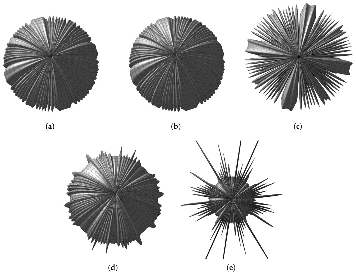
Figure 7.
Superpolar catenoids generated using the Gielis Superformula (Equation (3)) for different parameter sets . The parameter values are indicated below each subfigure.
Figure 7.
Superpolar catenoids generated using the Gielis Superformula (Equation (3)) for different parameter sets . The parameter values are indicated below each subfigure.
Disclaimer/Publisher’s Note: The statements, opinions and data contained in all publications are solely those of the individual author(s) and contributor(s) and not of MDPI and/or the editor(s). MDPI and/or the editor(s) disclaim responsibility for any injury to people or property resulting from any ideas, methods, instructions or products referred to in the content. |
© 2026 by the authors. Licensee MDPI, Basel, Switzerland. This article is an open access article distributed under the terms and conditions of the Creative Commons Attribution (CC BY) license (http://creativecommons.org/licenses/by/4.0/).
Copyright: This open access article is published under a Creative Commons CC BY 4.0 license, which permit the free download, distribution, and reuse, provided that the author and preprint are cited in any reuse.