The Geometries of Causal Inference: Learning and Evaluating Counterfactual Neighborhoods

1. Introduction

Matching is one of the most intuitive strategies for causal inference from observational data: estimate an unobserved counterfactual by locating one or more units that received the alternative treatment but are otherwise sufficiently comparable. The apparent simplicity of this prescription hides a central modeling decision: what should “comparable” mean? Conventional nearest-neighbor matching usually measures similarity in covariate space. Propensity-score matching uses similarity in treatment-assignment probability. Modern representation-learning methods construct latent spaces; causal forests induce adaptive neighborhoods through recursive partitions; and learned-metric methods stretch covariates according to outcome relevance. Each method therefore defines, explicitly or implicitly, a geometry over the sample.

This paper argues that there is no single universally correct geometry for causal inference. The useful notion of closeness depends on the causal task. A representation that is excellent for predicting heterogeneous treatment effects need not identify good explicit counterfactual substitutes. Conversely, a representation designed for counterfactual matching need not be optimal for global balance, propensity estimation, or direct CATE prediction. The distinction matters because the same pair of units can be close under one causal geometry and far apart under another.

The motivating lineage is Ramachandra (2018), which proposed autoencoder embeddings for generalized causal neighbor matching and a deep propensity-score model, PropensityNet [1]. That work addressed the curse of dimensionality by learning a lower-dimensional manifold before matching. The present paper revisits a more fundamental question: what should the learned manifold preserve if its purpose is causal matching? Reconstruction-based geometry preserves observational structure, but observational structure can be dominated by variation that is irrelevant to treatment assignment or potential outcomes. The resulting manifold may be an excellent representation of the data and a poor representation of counterfactual substitutability.

We therefore distinguish a family of task-specific causal geometries and introduce counterfactual geometry as the geometry of explicit substitution across treatment worlds. Let μₐ(x)=E[Y(a)|X=x] denote the treatment-specific response surface and let τ(x)=μ₁(x)−μ₀(x) denote the conditional treatment effect. Under binary treatment, the ideal counterfactual geometry places two units near one another when both treatment-specific response surfaces are jointly similar. This differs sharply from treatment-effect geometry: two units can have nearly identical treatment effects while their response levels differ greatly. Two patients may each benefit by ten units from treatment while having baseline risks separated by ninety units; they are similar treatment responders but poor substitutes for one another’s missing potential outcomes.

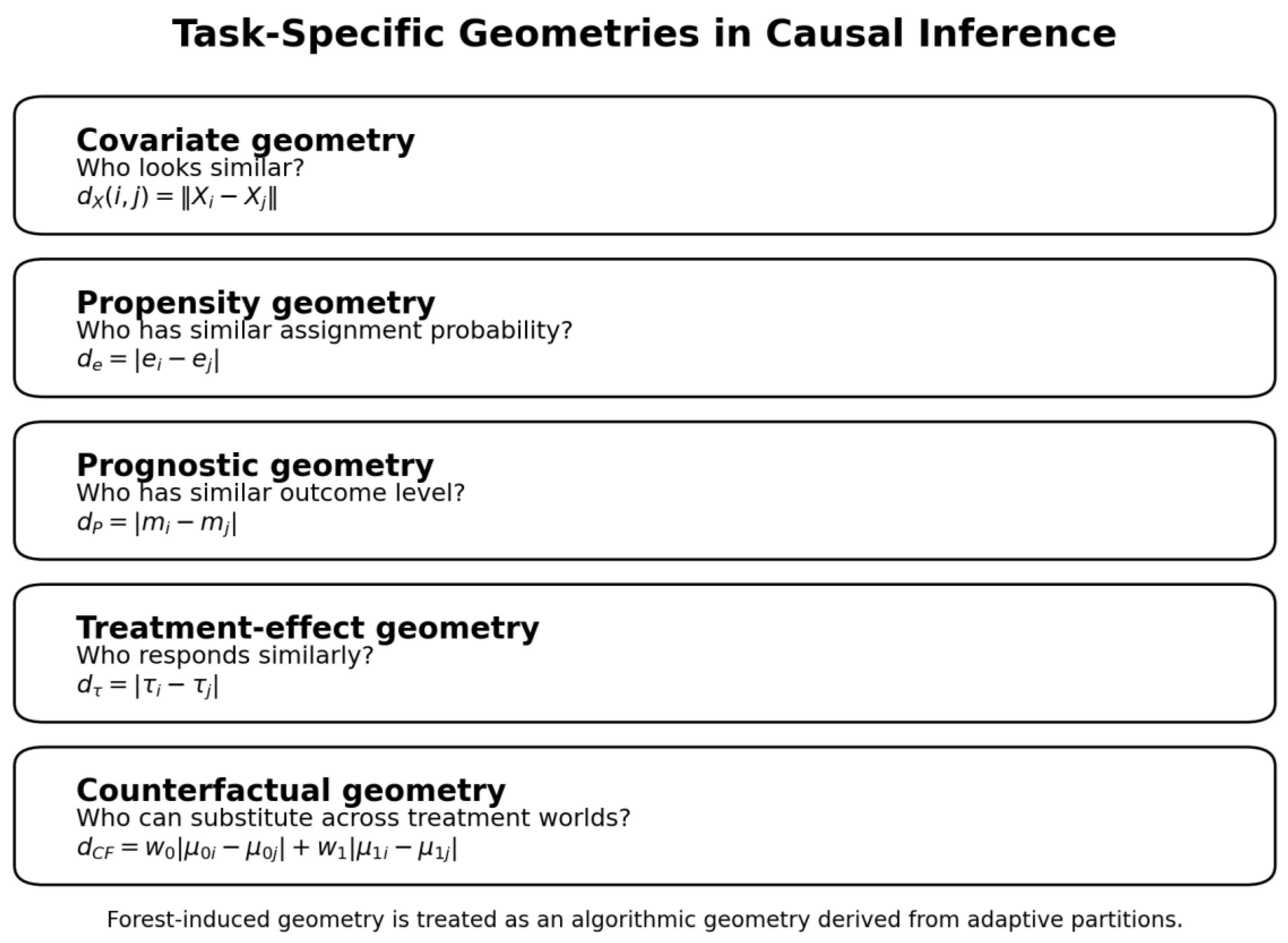
Figure 1. Task-specific geometries considered in this paper. “Causal geometry” is used as an umbrella description; counterfactual geometry is the proposed matching-specific object.

Figure 1. Task-specific geometries considered in this paper. “Causal geometry” is used as an umbrella description; counterfactual geometry is the proposed matching-specific object.

The paper makes four primary contributions. First, it develops a taxonomy separating covariate, propensity, prognostic, treatment-effect, forest-induced, and counterfactual geometries. Second, it defines counterfactual geometry directly through potential-outcome response surfaces and introduces Counterfactual Neighbor Regret (CNR), a geometry-specific diagnostic measuring how far a learned neighborhood falls short of the best counterfactual neighborhood available in the sample. Third, it provides a simple finite-sample regret bound that translates metric approximation error into counterfactual-neighbor regret and conditional matching bias. Fourth, it presents a set of stress-test experiments designed to separate observational similarity, treatment-effect similarity, and counterfactual substitutability. The experiments include high-dimensional nuisance geometry, hidden-confounding negative controls, treatment-effect versus counterfactual geometry, forest-neighborhood distillation, outcome-informed stretch proxies, neighborhood-size sensitivity, and a preliminary IHDP evaluation.

The broad term “causal geometry” is not new. It has been used in other contexts, including information-geometric analyses of causal models [20]. The novelty pursued here is narrower: a task-specific taxonomy for causal estimation, an explicit potential-outcome geometry for matching, and a regret criterion for evaluating whether a learned geometry actually selects near-oracle counterfactual neighborhoods.

2. Related Work and Proposed Novel Contributions

2.1. Matching, Learned Metrics, and Outcome-Informed Geometry

Classical matching emphasizes transparent comparisons but suffers in high dimensions and under irrelevant covariates [4]. Learned matching metrics address this weakness. MALTS learns an interpretable stretching of covariate space based on outcome-predictive importance, producing higher-quality almost-exact matches [13]. Model-to-Match generalizes this idea by learning variable importance from outcome models and then using the induced metric to create auditable matched groups [15]. Matched Machine Learning provides a broader framework for using learned metrics with matching while retaining inference and interpretability [14]. These works are among the closest intellectual predecessors of the present proposal.

The distinction here is not that prior methods fail to learn causally useful distances. Rather, they motivate the question of which causal object a distance should approximate. Counterfactual geometry is defined in response-surface space itself, and CNR evaluates selected neighborhoods relative to an oracle defined by missing potential outcomes. The proposed hybrid methods can therefore use outcome-informed stretching as a strong base geometry and add counterfactual coordinates rather than competing with learned matching as a category.

2.2. Representation Learning for Treatment-Effect Estimation

Johansson, Shalit, and Sontag introduced representation learning for counterfactual inference, and CFR-style methods later provided generalization bounds involving factual prediction error and distribution discrepancy between treated and control representations [5,6]. Perfect Match uses propensity-matched neighbors to augment neural-network minibatches [9]. Dragonnet jointly estimates outcome surfaces and propensity and adds targeted regularization motivated by semiparametric efficiency [11]. More recently, OR-learners combine learned representations with Neyman-orthogonal estimation and double robustness [17]. These methods primarily optimize representations for treatment-effect estimation or nuisance estimation, not for explicit auditability of counterfactual neighbors.

2.3. Forest-Induced Geometry

Causal forests and generalized random forests construct adaptive local weights targeted to heterogeneous causal quantities [7,10]. In this sense, forests induce an algorithmic geometry: two observations are “near” when they repeatedly receive large joint forest weights or co-occur in local partitions. This geometry is highly useful for local treatment-effect estimation. The present paper does not claim that causal forests lack causal geometry. Instead, it tests whether a geometry optimized for treatment-effect heterogeneity is necessarily a good geometry for explicit counterfactual substitution.

2.4. Manifold Geometry, Orthogonality, and Recent Neighborhood Ideas

GeoMatching explicitly studies the intrinsic Riemannian geometry of the covariate manifold and performs matching in the learned latent space [16]. This is particularly relevant to the 2018 autoencoder-matching lineage [1]. The present distinction is between geometry of the observational/confounder manifold and geometry of potential-outcome response surfaces: the two can coincide, but need not. Recent work on counterfactual covering for active learning develops factual and counterfactual covering radii that control treatment-effect risk under a data-acquisition problem [18]. Recent work on assessing HTE estimators emphasizes that evaluation is difficult because counterfactual outcomes are missing [19]. Concurrent 2026 work uses causally relevant neighborhoods for conformal prediction of individual causal effects [21]. These developments reinforce the importance of locality and support, while leaving open the specific problem addressed here: directly evaluating the quality of a matching geometry against the oracle counterfactual neighborhood available in semi-synthetic or simulated data.

Table 1. Positioning relative to the closest methodological families.

Method / family	Primary geometry or objective	Explicit matching?	Main distinction from this paper
Ramachandra 2018 [1]	Autoencoder/data-manifold + propensity	Yes	Geometry trained mainly for reconstruction or propensity, not potential-outcome substitution
CFR / balanced representations [5,6]	Distribution-balanced latent representation	No	Global representation balance rather than explicit local counterfactual-neighbor regret
Causal forest / GRF [7,10]	Adaptive heterogeneity-targeted forest weights	Implicit local weights	Targets local treatment effects; forest proximity need not minimize counterfactual substitution error
Perfect Match [9]	Propensity-matched training augmentation	Training-time	Uses matching to train CATE models; does not define oracle counterfactual-neighbor regret
MALTS [13]	Outcome-informed covariate stretching	Yes	Learns feature stretching; proposed framework defines a potential-outcome target geometry and CNR
Matched ML [14]	General learned metric for auditable matching	Yes	Broader framework; present work focuses on task-specific geometry and oracle-neighborhood regret
Model-to-Match [15]	Outcome-model variable importance	Yes	Variable-importance metric versus explicit response-surface counterfactual geometry
GeoMatching [16]	Intrinsic Riemannian data geometry	Yes	Observational/manifold geometry versus potential-outcome response geometry
OR-learners [17]	Orthogonal representation-level causal estimation	No/optional	Orthogonality is used for robust estimation, not claimed here as the geometry novelty
This work	Task-specific taxonomy; potential-outcome counterfactual geometry	Yes	Adds CNR, metric-regret bound, adaptive-neighborhood interpretation, and geometry comparisons

Table 1. Positioning relative to the closest methodological families.

Method / family	Primary geometry or objective	Explicit matching?	Main distinction from this paper
Ramachandra 2018 [1]	Autoencoder/data-manifold + propensity	Yes	Geometry trained mainly for reconstruction or propensity, not potential-outcome substitution
CFR / balanced representations [5,6]	Distribution-balanced latent representation	No	Global representation balance rather than explicit local counterfactual-neighbor regret
Causal forest / GRF [7,10]	Adaptive heterogeneity-targeted forest weights	Implicit local weights	Targets local treatment effects; forest proximity need not minimize counterfactual substitution error
Perfect Match [9]	Propensity-matched training augmentation	Training-time	Uses matching to train CATE models; does not define oracle counterfactual-neighbor regret
MALTS [13]	Outcome-informed covariate stretching	Yes	Learns feature stretching; proposed framework defines a potential-outcome target geometry and CNR
Matched ML [14]	General learned metric for auditable matching	Yes	Broader framework; present work focuses on task-specific geometry and oracle-neighborhood regret
Model-to-Match [15]	Outcome-model variable importance	Yes	Variable-importance metric versus explicit response-surface counterfactual geometry
GeoMatching [16]	Intrinsic Riemannian data geometry	Yes	Observational/manifold geometry versus potential-outcome response geometry
OR-learners [17]	Orthogonal representation-level causal estimation	No/optional	Orthogonality is used for robust estimation, not claimed here as the geometry novelty
This work	Task-specific taxonomy; potential-outcome counterfactual geometry	Yes	Adds CNR, metric-regret bound, adaptive-neighborhood interpretation, and geometry comparisons

3. Setup and Task-Specific Geometries

Let the observational sample contain pretreatment covariates, a binary treatment indicator, and an observed outcome for each unit. Let the two potential outcomes denote the outcomes under control and treatment. The consistency relationship between observed and potential outcomes is shown in Equation (1). We assume consistency, conditional exchangeability, and positivity when interpreting observational estimators causally. These assumptions are not relaxed by representation learning.

Y = A Y(1) + (1 − A) Y(0)

(1)

(Y, (0)Y(1))⊥A∣X

(2)

0 < e(X) = P(A = 1∣X) < 1

(3)

Define μₐ(x)=E[Y(a)|X=x] and τ(x)=μ₁(x)−μ₀(x). Different causal tasks then induce different notions of distance, summarized in the subsections below.

3.1. Covariate Geometry

d_X(i, j) = ‖X_i − X_j‖₂

(4)

Covariate geometry asks which units look similar observationally. It is intuitive but vulnerable to irrelevant or high-variance nuisance dimensions.

3.2. Propensity Geometry

𝒹_e(i, j) = |m(X_i) − m(X_j)|

(5)

Propensity geometry compresses the assignment mechanism into a scalar balancing score. It is appropriate for certain confounding-adjustment tasks but does not guarantee similarity of individual potential outcomes.

3.3. Prognostic Geometry

d_P(i, j) = |m(X_i) − m(X_j)|

(6)

Here m(x) denotes a prognostic score or expected outcome summary. Prognostic geometry is outcome-informed, but a single outcome summary may collapse treatment-specific response differences.

3.4. Treatment-Effect Geometry

d_τ(i, j) = |τ(X_i) − τ(X_j)|

(7)

Treatment-effect geometry asks which units respond similarly to treatment. This is central to heterogeneous treatment-effect estimation. It is not equivalent to counterfactual substitutability because equal contrasts do not imply equal levels.

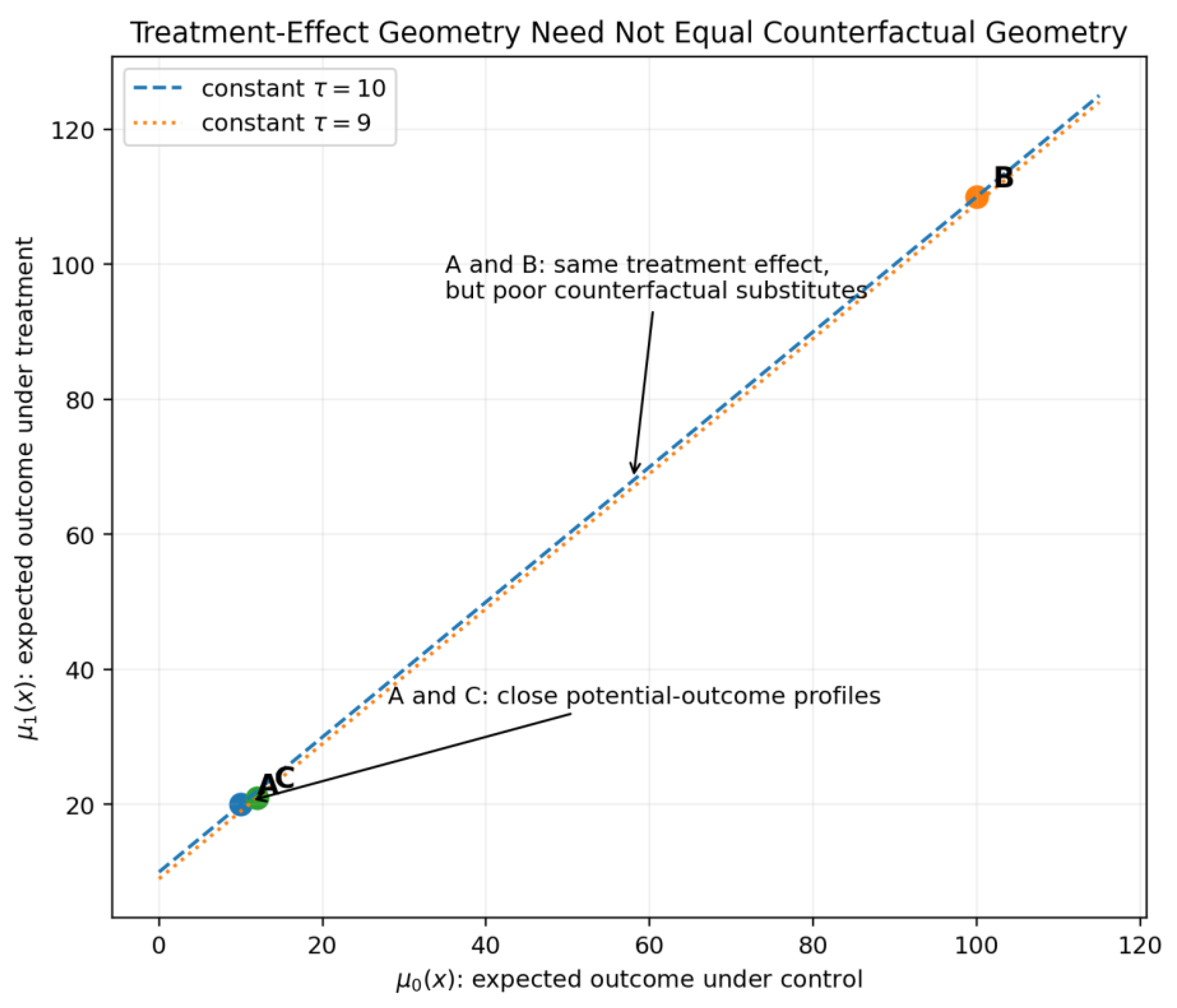
Figure 2. A and B have identical treatment effects but very different potential-outcome levels; A and C are substantially better counterfactual substitutes despite a small treatment-effect difference.

Figure 2. A and B have identical treatment effects but very different potential-outcome levels; A and C are substantially better counterfactual substitutes despite a small treatment-effect difference.

3.5. Forest-Induced Geometry

d_F(i, j) = 1 − P_F(i, j)

(8)

P_F(i,j) denotes a forest proximity or normalized local co-weight. This is an algorithmic geometry generated by adaptive partitions targeted to a causal quantity. Forest geometry may encode more than scalar CATE similarity, but its native objective is not necessarily explicit counterfactual substitution.

3.6. Counterfactual Geometry

$$d_{\mathit{CF}}^{*}\left(i,j\right)=w_0\left|{\mu }_0\left(X_i\right)-{\mu }_0\left(X_j\right)\right|+w_1\left|{\mu }_1\left(X_i\right)-{\mu }_1\left(X_j\right)\right|$$

(9)

Equation (9) defines the principal object of this paper. Two units are close if their expected behavior is similar under both treatment worlds. The weights w₀,w₁ can emphasize the treatment arm relevant to the estimand or be set symmetrically. For bidirectional matching, w₀=w₁ is a natural default.

Counterfactual geometry can be interpreted as the response-surface embedding defined by Equation (9). It is invariant to covariate dimensions that do not change the response surfaces. This yields the central conceptual distinction: a variable may dominate observational variance yet be irrelevant to counterfactual geometry, while a low-variance confounder may be essential.

4. Counterfactual Neighbor Regret

4.1. Definition

Treatment-effect metrics such as PEHE assess the downstream estimator, not the geometry itself. To evaluate whether a representation finds the right units to compare, we define Counterfactual Neighbor Regret. For each focal unit, consider the opposite-treatment candidate set, the oracle neighborhood that minimizes counterfactual loss, and the neighborhood returned by the learned geometry. The individual and average regret definitions are given in Equations (10) and (11).

$$R_{i,k}^{\mathit{CF}}=L_{\mathit{CF}}\left(i,{\widehat{N}}_k\left(i\right)\right)-L_{\mathit{CF}}\left(i,{\widehat{N}}_k^{*}\left(i\right)\right)$$

(10)

$$R_k^{\mathit{CF}}={\displaystyle \frac{1}{n}}{\sum }_i{R}_{i,k}^{\mathit{CF}}$$

(11)

In simulations and semi-synthetic data, counterfactual loss can use the missing potential outcome directly. For a treated unit, one natural loss is the absolute error between the selected control neighborhood’s mean untreated potential outcome and the focal unit’s untreated potential outcome; for an untreated unit the analogous loss uses the treated potential outcome. A response-surface version can use the oracle counterfactual metric in Equation (9). CNR is therefore a diagnostic of matching representation quality, not a replacement for PEHE, ATE error, calibration, or inferential coverage.

4.2. Metric Approximation and Neighbor-Regret Bound

Suppose a learned metric uniformly approximates the oracle counterfactual metric and that the neighbor-search procedure has bounded additive optimization error η. The formal uniform-approximation assumption is shown in Equation (12); Theorem 1 then carries the neighbor-search error explicitly into the regret bound.

$${}_{X,X^{\text{'}}}{}^{\sup }|\widehat{d}\left(X,X^{\text{'}}\right)-d^{*}\left(X,X^{\text{'}}\right)|\le \epsilon$$

(12)

Theorem 1 (Counterfactual-neighbor regret bound). Under the uniform approximation condition in (12), for every unit i,

$$d^{*}\left(X_i,X_j\right)-d^{*}\left(X_i,X_{j_i^{*}}\right)\le 2\epsilon +\eta$$

(13)

Proof. The proof applies the uniform approximation inequality to the learned neighbor, then uses approximate optimality of the neighbor search, and finally applies uniform approximation to the oracle neighbor. Chaining these three steps yields the regret bound in Equation (13).

4.3. Conditional Matching-Bias Corollary

For a treated unit, the conditional matching bias is the discrepancy between the focal unit’s untreated response surface and that of the selected control neighbor. Because the control component of the oracle counterfactual metric lower-bounds this discrepancy after weighting, Theorem 1 yields the bias bound in Equation (14).

$$\left|{\mathsf{Bias}}_i\left(0\right)\right|\le {\displaystyle \frac{d^{*}(X_i,X_{j_i^{*}})+2\epsilon +\eta }{w_0}}$$

(14)

An analogous result holds for untreated units with w₁. The bound decomposes matching error into three conceptually distinct terms: irreducible sample support (the oracle neighbor may itself be distant), metric-learning error ε, and search/optimization error η. This decomposition links geometry quality directly to causal matching bias.

4.4. K-Neighborhood Extension, Adaptive K, and Abstention

For k-neighbor matching, consider the average oracle counterfactual distance over a neighborhood. Under the same uniform-approximation logic, a learned approximate neighborhood inherits an additive geometry penalty plus search error. This suggests the bias–variance criterion in Equation (15).

$${\mathsf{MSE}}_i\left(k\right)\le \{{\displaystyle \frac{{\overline{d}}_i^{*}\left(k\right)+2\epsilon }{w}}{\}}^2+{\displaystyle \frac{{\sigma }_i^2}{K}}$$

(15)

Equation (15) motivates individualized neighborhood size: dense regions may support larger k and lower variance, while sparse regions require small k or abstention. A causal matching system can abstain when the best estimated local error bound exceeds a prespecified threshold. This gives support-aware selective causal inference a statistical rather than purely heuristic interpretation.

5. Learning Counterfactual Geometry

5.1. Direct Nuisance-Response Geometry

The simplest estimable approximation uses cross-fitted nuisance response surfaces and the propensity score. Their counterfactual-geometry representation is defined in Equation (16).

$${\mathcal{Z}}_{\mathit{CF}}\left(X\right)=[{\widehat{\mu }}_0\left(x\right),{\widehat{\mu }}_1\left(x\right),{\lambda }_e\widehat{e}(\mathrm{x}\left)\right]$$

(16)

Matching in the representation of Equation (16) directly operationalizes the counterfactual-geometry idea. The propensity coordinate is optional and should be interpreted as an overlap/comparability regularizer rather than as part of the ideal potential-outcome metric itself.

5.2. Outcome-Informed Stretching and Hybrid Geometry

The experiments indicate that strong outcome-informed learned metrics can outperform naive nuisance-response matching. We therefore treat learned stretching and counterfactual coordinates as complementary. Let the outcome-informed component be a stretched covariate representation, for example from MALTS- or Model-to-Match-like weighting. The hybrid representation is defined in Equation (17).

Z_H(X) = [Z_M(X), αZ_CF(X)]

(17)

The conceptual role of the hybrid is important: outcome-informed stretching can preserve prognostic structure that finite-sample nuisance estimates may miss, while the counterfactual component explicitly targets treatment-specific response surfaces. In this manuscript the implemented baselines are proxies inspired by MALTS and Model-to-Match, not exact reproductions of the published packages; definitive submission experiments should use the exact implementations.

5.3. Forest Teacher and Multi-Teacher Geometry

Forest proximities provide another teacher signal. A neural embedding f_θ(X) can be trained to preserve a convex combination of counterfactual-response distance and forest structural distance. Pure forest-to-neural distillation performed poorly in the designed stress test, while a modest forest contribution to a counterfactual objective improved performance in earlier experiments. This suggests a multi-teacher interpretation: forest partitions contribute nonlinear heterogeneity structure, but should not define counterfactual similarity by themselves.

5.4. Orthogonal Estimation Belongs Downstream

Early prototypes attempted to train geometry directly on individual doubly robust pseudo-outcomes. This failed in the stress tests because orthogonal pseudo-outcomes can be high variance at the individual level. The revised architecture therefore separates the roles of geometry and estimation: nuisance response surfaces and learned metrics construct neighborhoods; orthogonal scores and cross-fitting provide robustness for the final population-effect estimator. The AIPW score used for this downstream role is shown in Equation (18).

$${\mathsf{\Gamma }}_i=\widehat{{\mu }_1}\left(X_i\right)-\widehat{{\mu }_0}\left(X_i\right)+{\displaystyle \frac{A_i\left[Y_i-\widehat{{\mu }_1}\left(X_i\right)\right]}{\widehat{e}\left(X_i\right)}}-{\displaystyle \frac{\left(1-A_i\right)\left[Y_i-\widehat{{\mu }_0}\left(X_i\right)\right]}{1-\widehat{e}\left(X_i\right)}}$$

(18)

This division of labor is consistent with double/debiased machine learning: flexible nuisance models are combined with orthogonal scores and cross-fitting to reduce first-order sensitivity to nuisance estimation [8]. Orthogonality is therefore an estimation safeguard, not the claimed novelty of the geometry.

5.5. Orthogonal Counterfactual Coordinates as an Auxiliary Teacher

Section 5.4 deliberately rejected raw doubly robust treatment-effect pseudo-outcomes as the primary metric target. That negative result remains important, but it does not exhaust the useful role of orthogonality. A scalar DR treatment-effect score collapses the two response surfaces into their difference and therefore targets treatment-effect geometry, not counterfactual geometry. We instead define two arm-specific, cross-fitted orthogonal pseudo-outcomes, one for each potential-outcome response surface.

$${\varphi }_{1i}={\widehat{\mu }}_1\left(X_i\right)+{\displaystyle \frac{A_i}{\widehat{e}\left(X_i\right)}}\left\{Y_i-{\widehat{\mu }}_1\left(X_i\right)\right\}$$

$${\varphi }_{0i}={\widehat{\mu }}_0\left(X_i\right)+\begin{array}{c}{\displaystyle \frac{1-A_i}{1-\widehat{e}\left(X_i\right)}}\end{array}\left\{Y_i-{\widehat{\mu }}_0\left(X_i\right)\right\}$$

Here e(x)=P(A=1|X=x) is the propensity score and μ_a(x)=E[Y|A=a,X=x] is the treatment-specific outcome regression. All nuisance predictions used in the pseudo-outcomes are generated out of fold. The pair forms an orthogonal proxy for the two-dimensional counterfactual coordinate.

${\mathit{\Phi }}_i={\left({\mathit{\varphi }}_{0i},{\mathit{\varphi }}_{1i}\right)}^{\top },\mathbb{R}\left[{\mathit{\varphi }}_{\mathrm{a}i}\mid X_l=X\right]={\mu }_a\left(X\right)$Proposition 3 (conditional double robustness of OCC).For treatment arm a, under positivity and cross-fitting, E[φ_a|X=x]=μ_a(x) if either the propensity model is correct or the arm-specific outcome regression is correct. Thus the coordinate target inherits the familiar double-robust moment property arm by arm. This proposition concerns the conditional target of the pseudo-outcome; it does not imply that an individual φ_ai is a low-variance estimate of Y_i(a).

The last qualification is central. Raw φ_ai contains inverse-propensity-weighted residual noise and is unsuitable as a direct pairwise metric target in moderate samples. We therefore regress each arm-specific pseudo-outcome on X using a separate cross-fitted denoising learner and use the conditional predictions as orthogonal counterfactual coordinates.

$$r_{\mathrm{OCC}}\left(X\right)={\left({\tilde{\mu }}_0^{\mathrm{OCC}}\left(X\right),{\tilde{\mu }}_1^{\mathrm{OCC}}\left(X\right)\right)}^{\top }$$

OCC is best viewed as an auxiliary teacher rather than a replacement for the response-surface or outcome-informed metric. A practical hybrid concatenates an outcome-informed embedding, the ordinary nuisance-response coordinates, and the denoised OCC coordinates, with scale parameters selected out of fold against CNR or a prespecified matching loss.

$$r_{\mathrm{hybrid}}\left(\chi \right)={[S}_{\omega }\left(X\right),\lambda {\widehat{\mu }}_0\left(\chi \right),\lambda {\widehat{\mu }}_1\left(\chi \right),Y{\widehat{\mu }}_0^{\mathrm{OCC}}\left(\chi \right),Y{\widehat{\mu }}_1^{\mathrm{OCC}}\left(\chi \right)]$$

This construction reconciles two observations that would otherwise appear contradictory: orthogonal scores can be too noisy to define individual neighborhoods directly, yet orthogonality can still improve the geometry when used through arm-specific conditional denoising. It also preserves the paper’s distinction between treatment-effect geometry and counterfactual geometry: both μ0 and μ1 remain explicit coordinates.

6. Experiments

6.1. Design Principles

The experiments were designed to test the conceptual distinctions rather than to maximize performance on a single benchmark. We report repeated-seed means and standard deviations where available. The principal synthetic data-generating processes contain latent causal/prognostic coordinates and independent high-variance appearance coordinates. Treatment depends on causal coordinates, whereas high-dimensional nuisance variables dominate ordinary observational geometry. Because both potential outcomes are known in simulation, we can evaluate PEHE, true counterfactual-neighbor error, and CNR directly.

Several implemented comparators are explicitly labeled as proxies. The “causal-forest proxy” is a random forest trained on cross-fitted orthogonal pseudo-outcomes, with leaf co-occurrence used as proximity. “MALTS-style” and “Model-to-Match-style” proxies use outcome-informed feature stretching inspired by the corresponding published methods but are not exact package implementations.

6.2. Reconstruction and Nuisance-Geometry Stress Test

The first family of simulations asks whether a representation that preserves the dominant data manifold necessarily preserves counterfactual comparability. Low-dimensional causal variables determine treatment and potential outcomes, while increasingly many high-variance nuisance dimensions define an independent observational manifold. Raw matching, PCA/manifold matching, causal nuisance-space matching, and an orthogonal DR learner are compared as nuisance dimensionality increases.

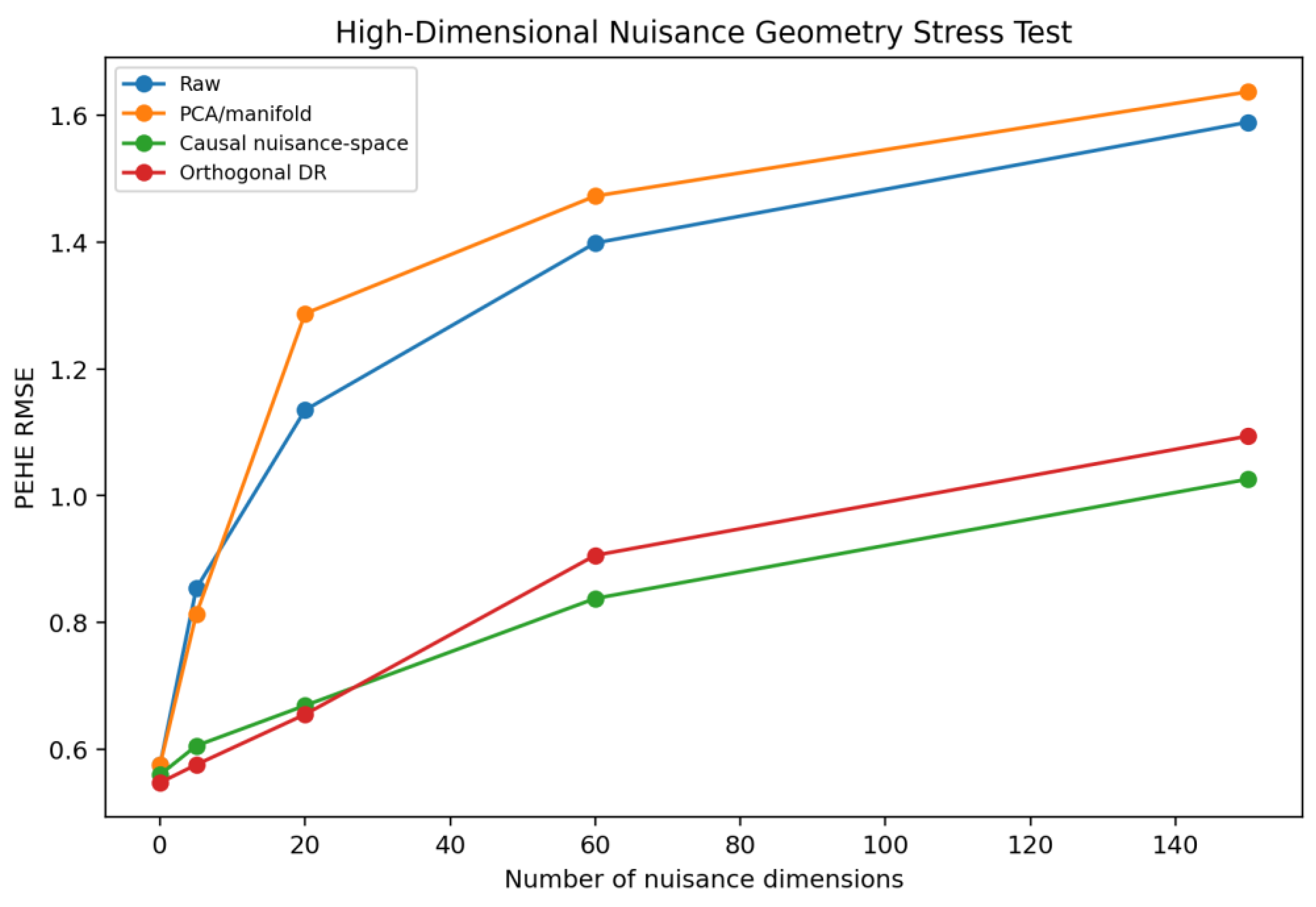
Figure 3. PEHE under increasing numbers of irrelevant nuisance dimensions. Data/manifold geometry degrades more rapidly than causally informed representations.

Figure 3. PEHE under increasing numbers of irrelevant nuisance dimensions. Data/manifold geometry degrades more rapidly than causally informed representations.

Table 2. Nuisance-dimensionality stress test: mean PEHE across three repeated seeds.

Nuisance dims	Causal-space match	Orthogonal DR	PCA/manifold	Raw match
0	0.560	0.548	0.575	0.575
5	0.606	0.576	0.813	0.854
20	0.669	0.655	1.287	1.135
60	0.838	0.906	1.473	1.399
150	1.026	1.094	1.637	1.589

Table 2. Nuisance-dimensionality stress test: mean PEHE across three repeated seeds.

Nuisance dims	Causal-space match	Orthogonal DR	PCA/manifold	Raw match
0	0.560	0.548	0.575	0.575
5	0.606	0.576	0.813	0.854
20	0.669	0.655	1.287	1.135
60	0.838	0.906	1.473	1.399
150	1.026	1.094	1.637	1.589

With no nuisance variables, methods are similar. As nuisance dimensionality increases, raw and PCA/manifold matching deteriorate substantially. At 150 nuisance dimensions, causal nuisance-space matching reaches mean PEHE 1.026 versus 1.589 for raw matching and 1.637 for PCA/manifold matching. The result supports the claim that recovering the dominant observational manifold is not equivalent to recovering a geometry useful for causal comparison.

6.3. Treatment-Effect Geometry Versus Counterfactual Geometry

A second simulation deliberately creates many units with similar treatment effects but very different prognostic levels. Treatment effect τ(x) depends primarily on one latent coordinate, while μ₀(x) contains a strong independent prognostic component. This construction makes equal-CATE/different-baseline pairs common and tests whether treatment-effect neighborhoods are valid counterfactual substitutes.

Forest-proximity neighbors had smaller mean treatment-effect differences than estimated counterfactual-geometry neighbors (approximately 0.31 versus 0.46–0.49 in these experiments), demonstrating that the forest proxy captured a treatment-effect-oriented neighborhood. Yet its true counterfactual-neighbor error was substantially larger (approximately 2.97 versus about 1.03 in the first forest experiment). The direct forest CATE predictor was much better than using forest proximity for matching, underscoring that a neighborhood useful internally for CATE estimation need not be a good explicit substitution geometry.

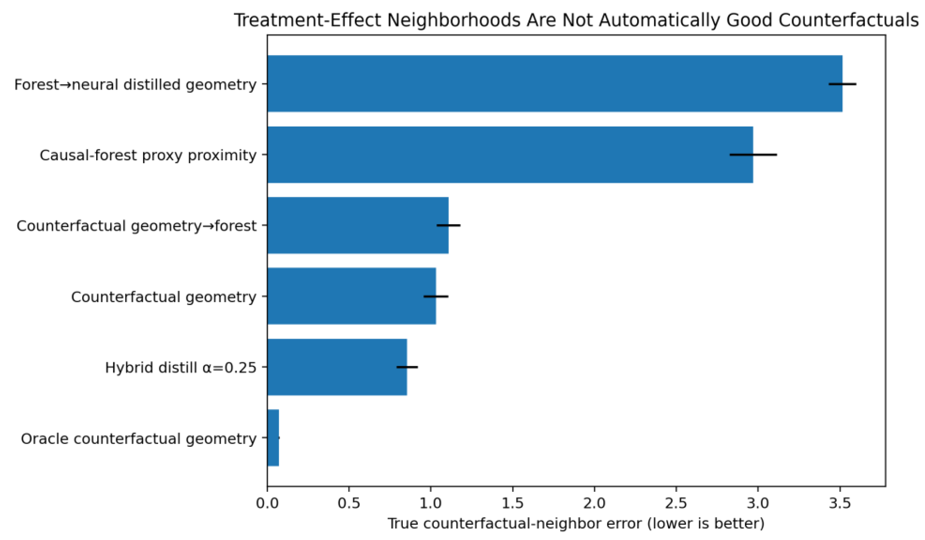
Table 3. Forest-induced versus counterfactual geometry. Lower is better for all metrics.

Method	PEHE	True CF-neighbor error	Neighbor CATE diff.
Oracle counterfactual geometry	0.465	0.071	0.174
Hybrid distill α=0.25	1.256	0.854	0.380
Counterfactual geometry	1.444	1.030	0.456
Counterfactual geometry→forest	1.559	1.108	0.469
Forest direct CATE prediction	1.676
Causal-forest proxy proximity	3.799	2.971	0.291
Forest→neural distilled geometry	4.533	3.515	0.313
Tau/orthogonal-score geometry	8.178	6.693	0.800

Table 3. Forest-induced versus counterfactual geometry. Lower is better for all metrics.

Method	PEHE	True CF-neighbor error	Neighbor CATE diff.
Oracle counterfactual geometry	0.465	0.071	0.174
Hybrid distill α=0.25	1.256	0.854	0.380
Counterfactual geometry	1.444	1.030	0.456
Counterfactual geometry→forest	1.559	1.108	0.469
Forest direct CATE prediction	1.676
Causal-forest proxy proximity	3.799	2.971	0.291
Forest→neural distilled geometry	4.533	3.515	0.313
Tau/orthogonal-score geometry	8.178	6.693	0.800

Figure 4. True counterfactual-neighbor error for counterfactual, forest-induced, distilled, and oracle geometries in the equal-CATE/different-baseline stress test.

Figure 4. True counterfactual-neighbor error for counterfactual, forest-induced, distilled, and oracle geometries in the equal-CATE/different-baseline stress test.

Pure forest-to-neural distillation also performed poorly, whereas an earlier hybrid neural distillation with a modest forest component improved over counterfactual geometry alone. A simple scalar CATE-coordinate augmentation did not reproduce that gain: increasing the CATE weight monotonically degraded both PEHE and CNR. This suggests that the useful forest signal is richer than scalar treatment-effect similarity and may involve nonlinear interaction structure in the partitions.

6.4. Broad Geometry Benchmark and Outcome-Informed Stretch Proxies

The oracle counterfactual geometry is decisively best, confirming that the target geometry is meaningful when available. However, the simple estimated response-surface geometry is not itself sufficient to beat strong outcome-informed stretching. The MALTS-style and Model-to-Match-style proxies achieve mean PEHE 0.878 and 0.905, respectively, versus 1.500 for the direct estimated counterfactual geometry. This is a constructive negative result: the matching only on [μ̂₀,μ̂₁,ê] does not universally dominate learned covariate metrics.

The hybrid representation combining an outcome-informed stretch proxy with explicit counterfactual coordinates improves further. The strongest tested hybrid achieves mean PEHE 0.847 and CNR₅ 0.623, compared with 0.878 and 0.650 for the MALTS-style proxy alone. The improvement is modest but consistent with the proposed interpretation: learned prognostic stretching and response-surface coordinates provide complementary information.

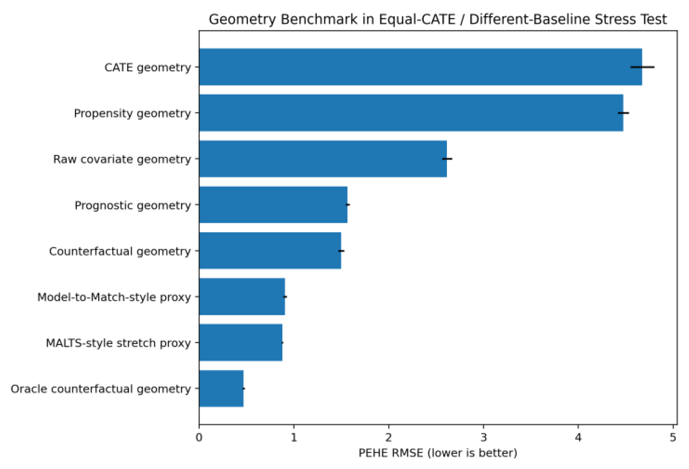
Table 4. Geometry benchmark in the equal-CATE/different-baseline stress test. CNR uses k=5.

Geometry / method	PEHE	CF-neighbor error	CNR₅
Oracle counterfactual geometry	0.468	0.368	0.345
MALTS-style stretch proxy	0.878	0.673	0.650
Model-to-Match-style proxy	0.905	0.688	0.665
Counterfactual geometry	1.500	1.125	1.103
Prognostic geometry	1.565	1.200	1.177
Raw covariate geometry	2.615	2.048	2.026
Propensity geometry	4.475	3.570	3.547
CATE geometry	4.676	3.727	3.704

Table 4. Geometry benchmark in the equal-CATE/different-baseline stress test. CNR uses k=5.

Geometry / method	PEHE	CF-neighbor error	CNR₅
Oracle counterfactual geometry	0.468	0.368	0.345
MALTS-style stretch proxy	0.878	0.673	0.650
Model-to-Match-style proxy	0.905	0.688	0.665
Counterfactual geometry	1.500	1.125	1.103
Prognostic geometry	1.565	1.200	1.177
Raw covariate geometry	2.615	2.048	2.026
Propensity geometry	4.475	3.570	3.547
CATE geometry	4.676	3.727	3.704

Figure 5. Broad geometry benchmark. The oracle potential-outcome geometry is strongest; outcome-informed stretch proxies outperform naive estimated response-surface matching in this finite-sample stress test.

Figure 5. Broad geometry benchmark. The oracle potential-outcome geometry is strongest; outcome-informed stretch proxies outperform naive estimated response-surface matching in this finite-sample stress test.

6.5. Counterfactual Neighbor Regret Across Neighborhood Size

For the hybrid, CNR decreases from 0.843 at k=1 to 0.612 at k=10 and then increases to 0.633 at k=20. PEHE follows a similar bias–variance pattern, reaching 0.847 at k=5 and 0.851 at k=10 before worsening to 0.913 at k=20. These patterns provide empirical support for adaptive neighborhood size rather than a globally fixed k.

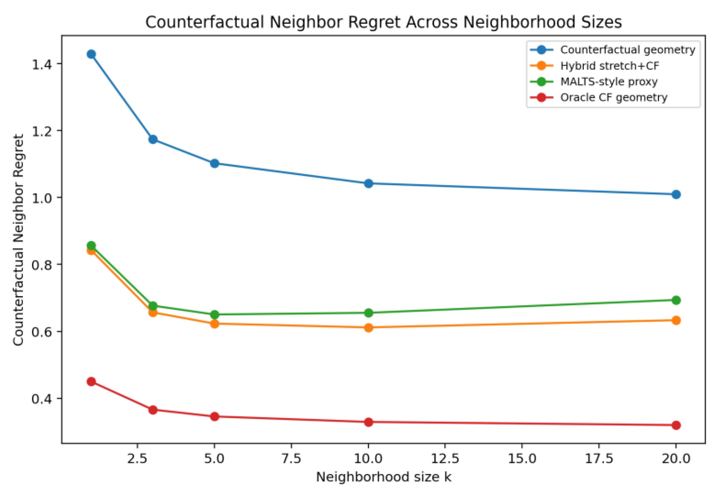
Figure 6. Counterfactual Neighbor Regret as neighborhood size increases. The hybrid retains lower regret than the MALTS-style proxy across tested k.

Figure 6. Counterfactual Neighbor Regret as neighborhood size increases. The hybrid retains lower regret than the MALTS-style proxy across tested k.

Table 5. Counterfactual Neighbor Regret as a function of k.

k	Estimated CF	MALTS-style	Hybrid	Oracle CF
1	1.429	0.856	0.843	0.450
3	1.174	0.677	0.657	0.366
5	1.103	0.650	0.623	0.345
10	1.042	0.655	0.612	0.329
20	1.010	0.694	0.633	0.320

Table 5. Counterfactual Neighbor Regret as a function of k.

k	Estimated CF	MALTS-style	Hybrid	Oracle CF
1	1.429	0.856	0.843	0.450
3	1.174	0.677	0.657	0.366
5	1.103	0.650	0.623	0.345
10	1.042	0.655	0.612	0.329
20	1.010	0.694	0.633	0.320

6.6. Hidden-Confounding Negative Control

A negative-control simulation introduces an unobserved variable affecting both treatment and outcome while withholding it from all estimators. All methods deteriorate sharply. For example, mean PEHE of causal nuisance-space matching rises from approximately 0.784 without hidden confounding to 1.795 with hidden confounding, while ATE absolute error rises from roughly 0.130 to 1.015. Orthogonal estimation also deteriorates. The result emphasizes that better geometry does not repair failed identification: representation learning cannot “learn away” a confounder that is not identified from the observed data under the assumed design.

6.7. Preliminary IHDP Evaluation

The preliminary IHDP experiment is deliberately reported as a reality check rather than as a definitive benchmark. Raw matching is competitive, and the learned counterfactual metric does not dominate. This is consistent with the paper’s task-specific thesis: when a modest-dimensional benchmark already provides an adequate geometry, a more elaborate learned geometry may offer little benefit. The result also motivates exact-method comparisons and a broader ACIC-style benchmark suite before submission.

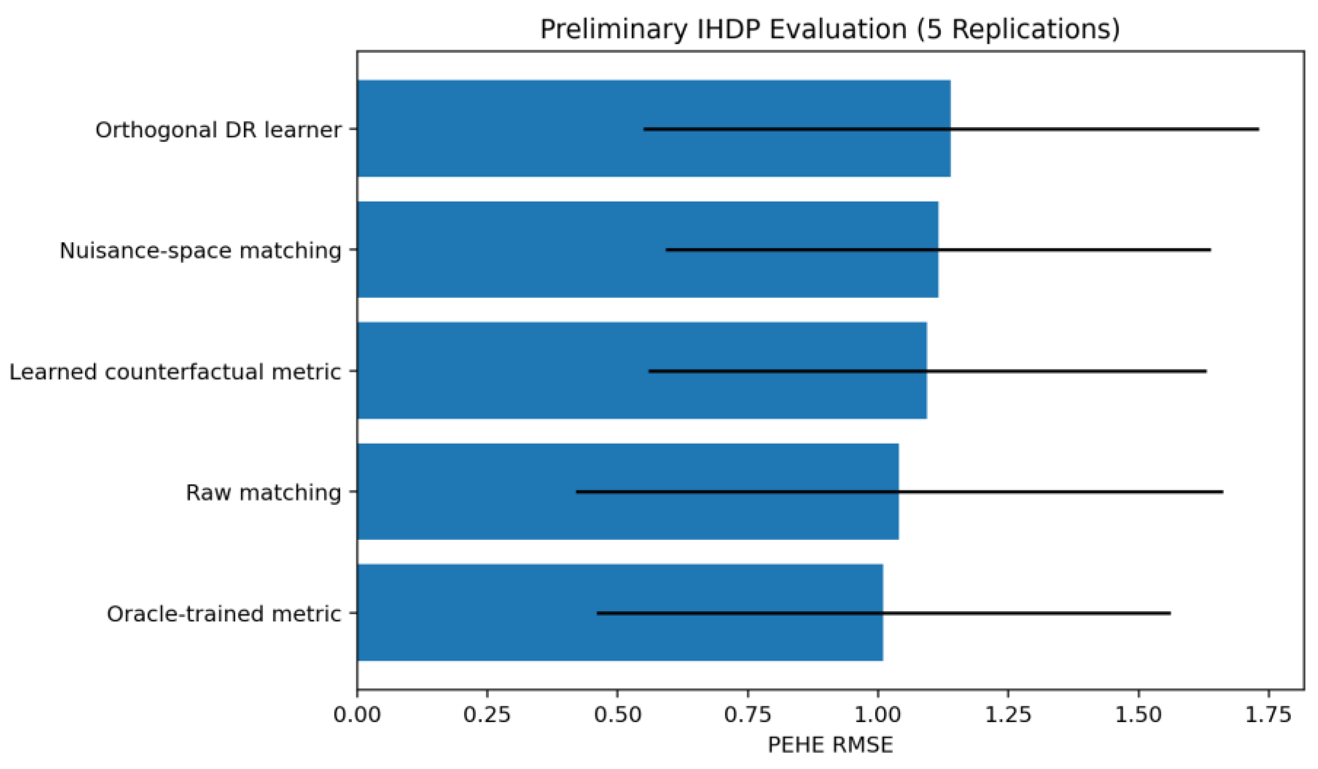
Table 6. Preliminary IHDP results (five accessible replications).

Method	PEHE	ATE absolute error
Learned counterfactual metric	1.094 ± 0.536	0.154 ± 0.163
Nuisance-space matching	1.115 ± 0.523	0.154 ± 0.181
Oracle-trained metric	1.010 ± 0.551	0.124 ± 0.101
Orthogonal DR learner	1.140 ± 0.591	0.303 ± 0.208
Raw matching	1.041 ± 0.622	0.119 ± 0.159

Table 6. Preliminary IHDP results (five accessible replications).

Method	PEHE	ATE absolute error
Learned counterfactual metric	1.094 ± 0.536	0.154 ± 0.163
Nuisance-space matching	1.115 ± 0.523	0.154 ± 0.181
Oracle-trained metric	1.010 ± 0.551	0.124 ± 0.101
Orthogonal DR learner	1.140 ± 0.591	0.303 ± 0.208
Raw matching	1.041 ± 0.622	0.119 ± 0.159

Figure 7. Preliminary five-replication IHDP evaluation. No geometry dominates universally on this small, standard benchmark.

Figure 7. Preliminary five-replication IHDP evaluation. No geometry dominates universally on this small, standard benchmark.

6.8. Orthogonal Counterfactual Coordinates Under Nuisance Misspecification

We added a targeted stress test to evaluate OCC in the setting it is designed to help. Across 20 Monte Carlo replications (n=700, p=10), treatment assignment followed a correctly specified logistic propensity model, while both treatment-specific outcome regressions were intentionally misspecified as linear ridge models despite nonlinear response surfaces. Outcomes had additive Gaussian noise (SD=0.7). Denoised OCC used a richer fixed nonlinear basis. For each geometry, every unit was matched to its nearest opposite-treatment neighbor. We report mean oracle counterfactual distance, CNR relative to the best available oracle opposite-treatment neighbor, and individual-effect PEHE.

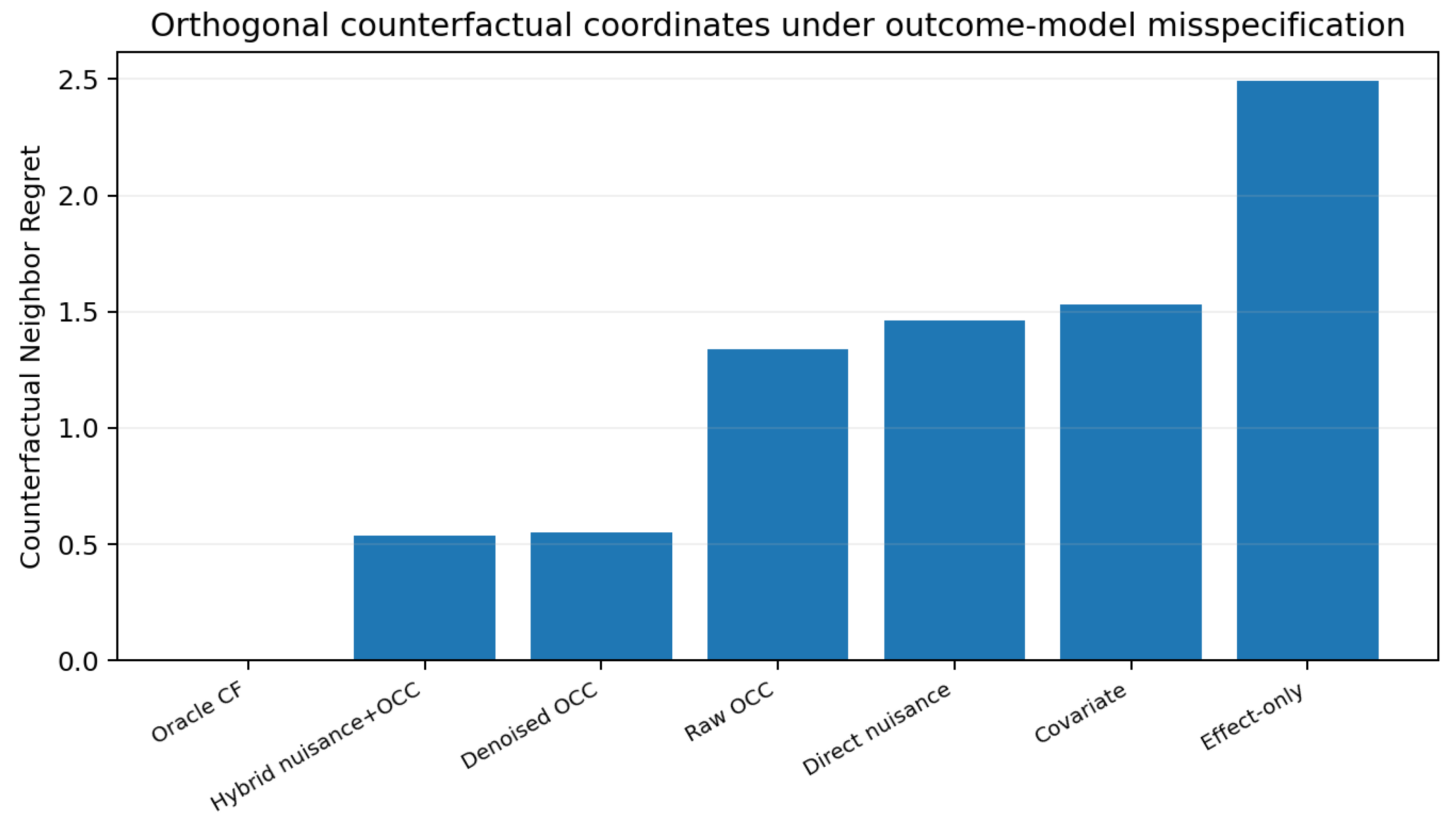
Table 7. Orthogonal counterfactual-coordinate stress test. Values are mean ± SD over 20 replications. Lower is better.

Geometry	CF distance	CNR	PEHE
Oracle counterfactual	0.125 ± 0.008	0.000	1.009 ± 0.039
Hybrid nuisance + OCC	0.662 ± 0.079	0.537 ± 0.076	1.145 ± 0.065
Denoised OCC	0.674 ± 0.124	0.549 ± 0.122	1.148 ± 0.073
Raw OCC	1.465 ± 0.055	1.340 ± 0.054	1.189 ± 0.113
Direct nuisance	1.586 ± 0.120	1.461 ± 0.119	1.801 ± 0.120
Covariate	1.656 ± 0.049	1.531 ± 0.045	1.795 ± 0.067
Effect-only	2.616 ± 0.170	2.491 ± 0.167	2.602 ± 0.195

Table 7. Orthogonal counterfactual-coordinate stress test. Values are mean ± SD over 20 replications. Lower is better.

Geometry	CF distance	CNR	PEHE
Oracle counterfactual	0.125 ± 0.008	0.000	1.009 ± 0.039
Hybrid nuisance + OCC	0.662 ± 0.079	0.537 ± 0.076	1.145 ± 0.065
Denoised OCC	0.674 ± 0.124	0.549 ± 0.122	1.148 ± 0.073
Raw OCC	1.465 ± 0.055	1.340 ± 0.054	1.189 ± 0.113
Direct nuisance	1.586 ± 0.120	1.461 ± 0.119	1.801 ± 0.120
Covariate	1.656 ± 0.049	1.531 ± 0.045	1.795 ± 0.067
Effect-only	2.616 ± 0.170	2.491 ± 0.167	2.602 ± 0.195

Figure 8. Counterfactual Neighbor Regret in the OCC nuisance-misspecification stress test.

Figure 8. Counterfactual Neighbor Regret in the OCC nuisance-misspecification stress test.

The result supports a narrower claim than “DR scores are good matching labels.” They are not: raw OCC remained noisy. The useful result is that conditional denoising of the two arm-specific orthogonal coordinates sharply improved counterfactual-neighbor quality when the direct outcome nuisances were misspecified. Denoised OCC reduced mean CNR from 1.461 to 0.549, and the hybrid nuisance+OCC representation reduced it slightly further to 0.537. The experiment therefore motivates OCC as a robustness-oriented auxiliary geometry teacher, while retaining the negative result for raw individual orthogonal scores.

7. Discussion

7.1. No Single Geometry for Causal Inference

The experiments support a more nuanced view of causal representation learning. “Causal similarity” is not one object. Propensity geometry describes similarity in the assignment mechanism; prognostic geometry describes similarity in expected outcome level; treatment-effect geometry describes similarity in treatment response; forest geometry reflects algorithmically adaptive local structure; counterfactual geometry describes substitutability across treatment worlds. A representation can be excellent under one criterion and poor under another.

This distinction is particularly important when interpretable matching is the downstream operation. If the goal is to show which untreated subjects provide evidence for a treated subject’s missing outcome, the geometry should be judged by the quality of those substitutes. PEHE alone cannot diagnose whether a model got the right answer for the right neighborhood. CNR is designed to expose that difference in settings where oracle potential outcomes are known.

7.2. Relationship to Causal Forests

Causal forests are not competitors merely because they induce neighborhoods. Their adaptive weights are constructed to estimate heterogeneous effects and can be statistically efficient for that purpose [7,10]. The designed equal-CATE/different-baseline experiment shows why forest proximity should not automatically be reinterpreted as a counterfactual matching metric. The forest’s direct CATE predictions were much better than matching on its induced proximity. Thus the result is not “counterfactual geometry beats causal forests”; it is “the geometry used for one task should not be assumed to solve another.”

7.3. Relationship to MALTS and Model-to-Match

MALTS and Model-to-Match are especially close because they already learn outcome-informed matching metrics [13,15]. The strong performance of our proxies is therefore not an inconvenience but an important constraint on the novelty claim. The likely contribution is not another generic learned metric. Instead, counterfactual geometry provides an estimand-specific target and CNR provides a geometry-specific evaluation criterion. The most promising empirical direction is hybridization: retain strong outcome-informed covariate stretching while adding response-surface coordinates and support-aware neighborhood selection.

7.4. Why Raw Orthogonal Pseudo-Outcomes Are Not the Primary Metric Target

The original negative result remains: direct pairwise matching on noisy doubly robust pseudo-outcomes performs poorly because orthogonality protects averages or appropriate regressions, not individual labels. The OCC extension clarifies the constructive alternative. Arm-specific orthogonal pseudo-outcomes can be cross-fitted, denoised conditionally on X, and used as auxiliary teachers for the two response-surface coordinates. In the nuisance-misspecification stress test this substantially lowered CNR. Thus orthogonality still belongs downstream of raw individual labels, but it can inform geometry after conditional denoising rather than being restricted only to the final ATE score.

7.5. Interpretability and Selective Causal Inference

Matching retains an advantage over black-box CATE prediction: an estimate can be accompanied by the actual opposite-treatment units that support it. Counterfactual geometry adds an explicit language for auditing those neighbors. The adaptive-k bound further suggests a principled abstention policy: if the best available counterfactual neighborhood remains distant, the method should report insufficient local counterfactual support rather than a falsely precise individualized effect.

8. Limitations of Our Study

First, the most compelling geometry metrics require simulated or semi-synthetic data where both potential outcomes or their response surfaces are available. CNR cannot be directly observed in ordinary real-world observational data. In practice, it can be used for benchmark development, model selection under semi-synthetic designs, and controlled stress tests; real-data validation must rely on indirect diagnostics, trial anchoring, sensitivity analysis, or external outcomes.

Second, the present empirical study includes proxy implementations inspired by MALTS, Model-to-Match, and causal-forest proximity. These results should not be interpreted as definitive superiority over the published algorithms.

Third, the theorem uses a strong uniform metric approximation condition. It is intended as a clean conceptual result linking geometry error to matching bias, not as a complete asymptotic theory for a particular neural metric learner. Stronger theory should derive rates for estimated response surfaces, neighborhood selection, and cross-fitting under explicit smoothness and overlap assumptions.

Finally, no geometry solves unmeasured confounding. If conditional exchangeability fails, a representation can produce visually convincing neighborhoods while the causal comparison remains invalid. The hidden-confounding negative control is included specifically to prevent an overly strong interpretation of deep or learned representations.

9. Extensions

9.1. Multi-Treatment Counterfactual Geometry

$$d_{\mathit{CF}}^{*}\left(i,j\right)={\displaystyle \sum _{a=1}^K}{w}_a\left|{\mu }_a\left(X_i\right)-{\mu }_a\left(X_i\right)\right|$$

(19)

For K treatments, counterfactual geometry naturally extends to the vector of treatment-specific response surfaces. This may be especially useful when a scalar propensity or treatment-effect summary is insufficient to describe comparability across several interventions.

9.2. Multimodal and High-Dimensional Counterfactual Geometry

The original motivation for deep matching becomes most relevant when X contains images, text, trajectories, or other structured high-dimensional measurements. A neural encoder can be trained jointly with response-surface heads and metric objectives so that generic appearance variation is compressed while treatment-specific response structure is preserved. Such settings may provide a clearer advantage for deep geometry learning than small tabular benchmarks.

9.3. Geometry-Aware Uncertainty

The support term in the bias bound can be combined with conformal, bootstrap, or semiparametric uncertainty. A useful system would report both treatment-effect uncertainty and neighborhood support. These are different uncertainties: the first concerns estimation variability, while the second concerns whether comparable opposite-treatment evidence exists locally.

10. Conclusions

This paper reframes causal representation learning as a problem of task-specific geometry. Covariate, propensity, prognostic, treatment-effect, forest-induced, and counterfactual geometries answer different questions about similarity. The distinction is not semantic: simulations show that units with similar treatment effects can be poor counterfactual substitutes, and forest-induced neighborhoods useful for CATE prediction can perform poorly when repurposed for explicit matching.

For matching, we propose counterfactual geometry based on joint similarity of treatment-specific response surfaces and Counterfactual Neighbor Regret as a direct measure of neighborhood quality relative to the oracle support available in the sample. A simple regret theorem connects metric approximation to matching bias, and an adaptive-k interpretation links geometry to selective causal inference. The experiments also provide an important caution: simple estimated response-surface geometry is not automatically better than strong outcome-informed learned metrics. The best tested direction is hybrid, combining outcome-informed stretching with explicit counterfactual coordinates. The new OCC extension adds a robustness-oriented route to learning these coordinates: arm-specific orthogonal pseudo-outcomes are denoised and used as auxiliary teachers, improving neighborhood quality under outcome-model misspecification without collapsing counterfactual geometry to a scalar treatment-effect score.

The resulting message is broader than a single neural architecture: representations should be evaluated by the causal operation they are meant to support. For explicit matching, the relevant question is not merely whether two units look alike or respond similarly, but whether one can credibly stand in for the other in the treatment world that was not observed.

References

- Ramachandra, V. Deep Learning for Causal Inference. arXiv 2018, arXiv:1803.00149. [Google Scholar]
- Rubin, D. B. Estimating causal effects of treatments in randomized and nonrandomized studies. J. Educ. Psychol. 1974, vol. 66(no. 5), 688–701. [Google Scholar] [CrossRef]
- Rosenbaum, P. R.; Rubin, D. B. The central role of the propensity score in observational studies for causal effects. Biometrika 1983, vol. 70(no. 1), 41–55. [Google Scholar] [CrossRef]
- Abadie; Imbens, G. W. Large sample properties of matching estimators for average treatment effects. Econometrica 2006, vol. 74(no. 1), 235–267. [Google Scholar] [CrossRef]
- Johansson, F.; Shalit, U.; Sontag, D. Learning representations for counterfactual inference. Proceedings of ICML, PMLR, 2016; 48, pp. 3020–3029. [Google Scholar]
- Shalit, U.; Johansson, F. D.; Sontag, D. Estimating individual treatment effect: Generalization bounds and algorithms. Proceedings of ICML, PMLR 70, 2017; pp. 3076–3085. [Google Scholar]
- Wager, S.; Athey, S. Estimation and inference of heterogeneous treatment effects using random forests. J. Am. Stat. Assoc. 2018, vol. 113(no. 523), 1228–1242. [Google Scholar] [CrossRef]
- Chernozhukov, V.; Chetverikov, D.; Demirer, M.; Duflo, E.; Hansen, C.; Newey, W.; Robins, J. Double/debiased machine learning for treatment and structural parameters. Econom. J. 2018, vol. 21(no. 1), C1–C68. [Google Scholar] [CrossRef]
- Schwab, P.; Linhardt, L.; Karlen, W. Perfect Match: A simple method for learning representations for counterfactual inference with neural networks. arXiv 2018, arXiv:1810.00656. [Google Scholar]
- Athey, S.; Tibshirani, J.; Wager, S. Generalized random forests. Ann. Stat. 2019, vol. 47(no. 2), 1148–1178. [Google Scholar] [CrossRef]
- Shi, C.; Blei, D. M.; Veitch, V. Adapting neural networks for the estimation of treatment effects. Adv. Neural Inf. Process. Syst. 2019, 32. [Google Scholar]
- Zhang, Y.; Bellot, A.; van der Schaar, M. Learning overlapping representations for the estimation of individualized treatment effects. Proceedings of AISTATS, PMLR 108, 2020; pp. 1005–1014. [Google Scholar]
- Parikh, H.; Rudin, C.; Volfovsky, A. MALTS: Matching After Learning to Stretch. J. Mach. Learn. Res. 2022, vol. 23(no. 240), 1–42. [Google Scholar]
- Morucci, M.; Rudin, C.; Volfovsky, A. Matched Machine Learning: A generalized framework for treatment effect inference with learned metrics. arXiv 2023, arXiv:2304.01316. [Google Scholar]
- Lanners, Q.; Parikh, H.; Volfovsky, A.; Rudin, C.; Page, D. Variable importance matching for causal inference. Proceedings of UAI, PMLR, 2023; 216, pp. 1174–1184. [Google Scholar]
- Pradier, M. F.; González, J. Beyond Flatland: A geometric take on matching methods for treatment effect estimation. Proceedings of CLeaR, PMLR, 2025; 275, pp. 1086–1115. [Google Scholar]
- Melnychuk, V.; Frauen, D.; Schweisthal, J.; Feuerriegel, S. Orthogonal Representation Learning for Estimating Causal Quantities. arXiv 2025, arXiv:2502.04274. [Google Scholar]
- Wen, H.; Chen, T.; Gong, M.; Chai, L. K.; Sadiq, S.; Yin, H. Enhancing treatment effect estimation via active learning: A counterfactual covering perspective. Proceedings of ICML, PMLR 267, 2025; pp. 66437–66466. [Google Scholar]
- Gao, Z. Trustworthy assessment of heterogeneous treatment effect estimator via analysis of relative error. Proc. AISTATS PMLR 2025, 258, 1063–1071. [Google Scholar]
- Chvykov, P.; Hoel, E. Causal Geometry. arXiv 2020, arXiv:2010.09390. [Google Scholar]
- Delbianco, F.; Tohmé, F. Local conformal prediction for individual causal effects. arXiv 2026, arXiv:2608.09612. [Google Scholar]
- Louizos, C.; Shalit, U.; Mooij, J. M.; Sontag, D.; Zemel, R.; Welling, M. Causal effect inference with deep latent-variable models. Adv. Neural Inf. Process. Syst. 2017, 30. [Google Scholar]
Disclaimer/Publisher’s Note: The statements, opinions and data contained in all publications are solely those of the individual author(s) and contributor(s) and not of MDPI and/or the editor(s). MDPI and/or the editor(s) disclaim responsibility for any injury to people or property resulting from any ideas, methods, instructions or products referred to in the content. |
© 2026 by the authors. Licensee MDPI, Basel, Switzerland. This article is an open access article distributed under the terms and conditions of the Creative Commons Attribution (CC BY) license (http://creativecommons.org/licenses/by/4.0/).
Copyright: This open access article is published under a Creative Commons CC BY 4.0 license, which permit the free download, distribution, and reuse, provided that the author and preprint are cited in any reuse.