

Submitted:
25 September 2026
Posted:
29 September 2026
You are already at the latest version
Abstract
Meteorology drives the day-to-day pollution variation behind short-term health effects, and its misattribution biases exposure estimates and trend normalisation. Wind speed and boundary-layer height (BLH), the two main dispersion controls, are strongly collinear and their relative roles are contested. We quantified the variance unique to each with semi-partial R² for NO₂, O₃, PM₁₀ and PM₂.₅ in France's ten largest cities over 2018–2025, across four frames, from pooled levels to deseasonalized, de-trended anomalies, checked with generalized additive models. Wind and BLH covary strongly (mean r ≈ 0.70, 0.81 on anomalies). On pooled levels, BLH carries four (NO₂, O₃) to nine (particulate matter) times the unique variance of wind, whereas their raw correlations with the primary pollutants differ by a factor of only 1.3 to 1.4. This lead is robust for particulate matter. For O₃, temperature dominates and humidity then exceeds BLH, plausibly a photochemical signal. For NO₂ it is partly seasonal: on anomalies the two become comparable, and wind leads only in cities with coherent regional winds. The contrasts yield a three-type typology, ventilation-controlled, transitional and boundary-layer-controlled, which predicts the meteorological covariate each city needs. A single meteorological adjustment is therefore inadequate across cities, and BLH should become a first-tier predictor.
Keywords:
air pollution
; boundary-layer height
; wind speed
; temperature
; humidity
; semi-partial variance
; deseasonalisation
; city typology
; exposure assessment
; meteorological normalisation
1. Introduction
Ambient air pollution is the leading environmental risk to human health. The Global Burden of Disease analysis for 2015 attributes 4.2 million premature deaths a year worldwide to ambient fine particulate matter, plus a further 254 000 to ozone, predominantly through cardiovascular and respiratory disease [1], and the most recent update confirms ambient particulate matter among the leading global risk factors [2]. The corresponding loss of life expectancy is comparable to that of the major behavioural risk factors [3]. In Europe the burden is concentrated in cities. A health impact assessment across 969 European cities estimates that compliance with the air quality guidelines then in force would prevent about 51 000 deaths a year for PM₂.₅ alone [4]. Large European cohorts confirm adverse effects at the low concentrations typical of western European cities, and find no evidence of a threshold below which risk disappears [5,6]. Nitrogen dioxide (NO₂), ozone (O₃) and particulate matter (PM₁₀ and PM₂.₅) remain the regulated pollutants of greatest public-health relevance. The systematic reviews that underpin the current guideline values quantify their short-term and long-term associations with mortality [7,8,9,10], and traffic-related exposure, dominant in city centres, carries its own documented effects [11]. Multi-city time-series analyses show that the day-to-day variation of concentration, and not only its long-term mean, is associated with daily mortality for particulate matter [12], for ozone [13] and for NO₂ [14]. This is the variation that meteorology modulates, which is why its correct attribution matters beyond atmospheric science.
While emissions set the source strength, the day-to-day and seasonal variability of surface concentrations is governed substantially by meteorology, through dilution, dispersion, transport and deposition, and, for O₃, photochemistry [15,16,17]. Daily meteorological variables alone can explain up to roughly half of the day-to-day variance of fine particulate matter [18]. Two meteorological controls dominate the dilution of primary pollutants. The height of the atmospheric (planetary) boundary layer (BLH) sets the vertical volume into which surface emissions are mixed. A shallow, stable layer concentrates pollutants near the ground, whereas a deep, well-mixed layer dilutes them [15,19,20,21,22]. Horizontal wind speed ventilates the urban canopy and advects pollutants away from their sources [16,23]. Both quantities are inversely related to primary-pollutant concentrations, and pollution episodes typically coincide with shallow boundary layers, weak winds and persistent anticyclonic stagnation [20,24,25]. Their combination, the product of mixing depth and transport wind, called the ventilation coefficient, has indexed a region's pollution potential since Holzworth [26] and remains in use through formulations based on the ERA5 reanalysis [27]. ERA5 is the fifth-generation global atmospheric reanalysis of the European Centre for Medium-Range Weather Forecasts. It assimilates the historical observing system into a frozen forecast model and delivers a physically consistent, gap-free hourly record of surface and upper-air variables from 1940 onward, on a 0.25° grid [28].
These two controls are, however, strongly and physically coupled, and this coupling is the central problem the present study addresses. Mechanical and convective mixing both deepen the boundary layer on windy, well-ventilated days, so wind speed and boundary-layer height covary on diurnal, synoptic and seasonal timescales [29]. The two variables nonetheless represent physically distinct dispersion pathways, horizontal advection for wind, vertical mixing volume for BLH. The literature remains divided on their relative importance. Some studies emphasise ventilation, others vertical mixing, often on the basis of univariate correlations or variable-importance rankings that do not isolate the variance unique to each driver, and that therefore attribute the shared variance to whichever variable is included [20,30,31,32]. When two collinear predictors compete, a poorly specified model systematically overstates the role of the one it retains [33]. The methodological consequence is that univariate wind regression cannot be read as capturing horizontal advection alone, because a large part of its apparent signal is variance shared with boundary-layer height. Conversely, once that shared part is handled, the wind term becomes usable: isolating the wind contribution to recover the local-source component of a PM₂.₅ trend has been demonstrated for Paris [34].
A further reason to treat the two pathways separately is that gases and particles are not transported and removed in the same way. For a gas such as NO₂ or O₃, dispersion is a matter of advection, mixing volume and chemistry, and the atmospheric lifetime is short and set by photochemistry [35]. Particles add mechanisms that have no gaseous counterpart. Their gravitational settling and dry deposition velocities depend on diameter, density and shape [36]. Their removal by precipitation is strongly size-selective, and observations in French cities show that rain scavenges coarse particles efficiently while leaving the accumulation mode almost untouched [37]. Their radiative properties feedback on the boundary layer that disperses them, since absorbing aerosols warm the upper layer and suppress its growth [38,39,40]. Their residence time is consequently longer and more variable than that of the reactive gases [41]. A decomposition of meteorological control should therefore be expected to differ between the gaseous and the particulate species, and this expectation is borne out below.
Compounding this, boundary-layer height has been largely absent from operational and empirical urban air-quality analysis in Europe, despite its physical primacy. Its role in particulate accumulation has been documented mainly for Chinese megacities [20,42], and its variability over European sites chiefly in dedicated lidar, ceilometer and profiling campaigns [43,44,45]. ERA5 now provides a continuous, hourly boundary-layer-height field co-located with every city [28,46], making a systematic continental treatment feasible. Normalisation studies that already include boundary-layer height hint that distinct regimes drive different pollutants [30,47], yet a systematic multi-city decomposition of the unique wind and boundary-layer contributions, across pollutants and frames, is lacking.
The apparent answer is, moreover, sensitive to two analytical choices that are seldom examined together. The first is whether the seasonal co-cycling of meteorology and pollution is controlled. The second is the temporal scale at which the series are aggregated. Over Europe a few weather regimes alone explain 60 to 80% of the monthly variability of regional pollution [48]. Either choice can flip the apparent driver [49].
Here we quantify the unique contributions of wind speed, boundary-layer height and six other surface meteorological drivers to daily concentrations of NO₂, O₃, PM₁₀ and PM₂.₅ across ten major French cities (Paris, Lyon, Marseille, Toulouse, Lille, Nice, Bordeaux, Montpellier, Nantes and Strasbourg, Figure 1) over 2018–2025. The six other drivers are air temperature, surface pressure, relative humidity, total cloud cover, precipitation and wind direction. We use a validated, harmonised daily dataset (2922 days per city, approximately 270 000 observations) built from urban-background measurements of the French national air-quality database Geod'air [50], together with ERA5 boundary-layer height and surface meteorology [28], and an hourly record of around 7 million observations across the four pollutants and eight meteorological variables.
We address three questions. (i) Do wind and BLH carry distinct, separable information, and how does their balance differ among pollutants? (ii) To what extent is the dominance of boundary-layer dynamics an artifact of seasonal co-cycling rather than a within-season coupling? (iii) Does the wind/BLH balance organise into an interpretable urban-meteorological typology across cities? We show that the answers revise the simple reading in which boundary-layer dynamics govern day-to-day pollution into a picture specific to each pollutant and each city, with the wind–boundary-layer dissociation as the headline finding and with direct implications for exposure modelling and for the meteorological normalisation of air-quality trends. To our knowledge, no multi-city decomposition of the unique wind and boundary-layer contributions has ever been made for European cities under both seasonal and trend control, and none has been turned into a city typology. That typology is the most practical product of the study. It is meteorological rather than merely geographic, and it states which covariate, ventilation or vertical mixing, a given city needs.
2. Materials and Methods
2.1. Study Area and Data
2.1.1. Cities and Meteorological Setting
We study the ten most populous French cities, which span contrasted climatic and topographic settings: flat oceanic plains (Lille, Nantes, Paris), continental valleys and plains (Strasbourg in the Rhine plain, Lyon in the Rhône–Saône corridor, Toulouse in the Garonne plain, reached by the Autan from the south-east and the Tramontane from the north-west), an Atlantic estuary (Bordeaux), Mediterranean coasts with powerful regional winds (Marseille, swept by the Mistral, a strong cold dry north-westerly wind, and Montpellier, by the Tramontane) and a sheltered coastal bay (Nice). The Mistral and the Tramontane are the two coherent regional wind systems of the French Mediterranean, and their climatology and their effect on pollution transport and vertical mixing are documented [51,52]. The channelling of the lower Rhône valley and its interaction with the sea breeze around Marseille are equally well characterised [53]. Table 1 lists the ten cities with their climate class, topographic setting and regional wind regime. Figure 1 maps their geographic distribution together with the mean boundary-layer and wind climatology.
2.1.2. Pollutant Data
Daily concentrations of NO₂, O₃, PM₁₀ and PM₂.₅ were obtained from Geod'air, the French national air-quality database, for 1 January 2018 to 31 December 2025 (2922 days per city) [50]. Geod'air is operated by Ineris under its mandate as the Laboratoire Central de Surveillance de la Qualité de l'Air (LCSQA) for the French ministry in charge of the environment. It consolidates the regulatory measurements of the eighteen accredited regional air-quality monitoring associations (AASQA), which operate the national reference network of about 550 fixed stations. The instruments, the siting criteria and the validation procedures follow the requirements of the European ambient air quality directive [54], recast in 2024 [55], and the national implementation guide [56]. The measurements used here are therefore normative regulatory data, not research-grade or low-cost sensor data.
Only urban-background stations were used (influence type = background, setting = urban). In the European framework, urban-background locations are defined as places in urban areas where levels are representative of the exposure of the general urban population [54], and the French classification guide defines a background measurement as one not significantly influenced by any single source, but rather by the integrated contribution of many sources over a spatial scale of several kilometres to several tens of kilometres [56]. Only officially validated measurements (validity flag = 1) were retained. Invalid, zero and negative values were discarded before averaging, a negative concentration being a calibration artefact rather than a measurement. Where a city has several urban-background stations, the daily value is the mean of the available validated, non-null station values (Paris seven stations, Lyon, Marseille and Strasbourg two to three stations each, and the remaining cities one station).
Using urban-background stations only is a deliberate choice with two consequences. Traffic-proximate measurements would overstate the apparent local ventilation signal. Urban-background sites, by design, integrate the urban air mass instead of sampling vehicular plumes, and therefore track synoptic-scale meteorology more closely.
2.1.3. Meteorological Data
All meteorological variables come from the ERA5 reanalysis [28]. ERA5 is provided on a regular 0.25° × 0.25° grid, about 28 km in latitude and, at the latitudes of the ten cities (43° N to 51° N), 18 to 20 km in longitude. For each city a single grid cell was used, the one co-located with the city centre, and all variables were extracted from that same cell and aggregated to daily means. No spatial averaging over the urban area was performed, since a 0.25° cell already covers an area of the order of the agglomeration itself. Units are homogeneous across the ten cities (°C, %, hPa, %, mm, km h⁻¹, °, m).
Boundary-layer height in ERA5 is diagnosed from a bulk Richardson-number criterion applied to the model profile [46]. Before use, we verified that each city is represented by a land grid point. For the coastal cities, the grid cell nearest the city centre initially returned by the extraction was in some cases a sea point. A sea point is recognisable by two signatures, a nearly flat diurnal cycle of BLH and a seasonal cycle in opposite phase to the land cycle, with maxima in winter instead of summer. Where such a cell was found, we moved the extraction to the nearest cell whose ERA5 land-sea mask value exceeds 0.5, checked that the diurnal amplitude and the seasonal phase had recovered their land signatures, and used that cell throughout. This correction matters, because a sea grid point inflates the apparent independent effect of wind. The full procedure and the affected cities are documented with the dataset.
The surface meteorological parameters extracted are wind speed at 10 m above the ground (km h⁻¹), air temperature and relative humidity at 2 m, surface pressure, total cloud cover and precipitation. These reanalysis fields enter our statistical regression models as explanatory variables, and are referred to as predictors only in that statistical sense. The primary statistical model uses the seven parameters available for all ten cities: wind speed, BLH, temperature, pressure, cloud cover, precipitation and relative humidity. The eighth variable, wind direction, a circular variable that a single linear coefficient cannot represent, is excluded from the primary linear model and examined separately (Section 2.2.5). Table 2 gives the 2018–2025 descriptive statistics of the pollutants and of the main meteorological parameters.
The concentration levels in Table 2 are moderate by international standards. Period means of PM₂.₅ range from 8.5 to 13.0 µg m⁻³ and of PM₁₀ from 14.8 to 20.1 µg m⁻³. They are several times lower than those of the Asian megacities where the boundary-layer control of particulate matter has mostly been documented [20,42]. They nonetheless exceed the current WHO guideline values of 5 µg m⁻³ for PM₂.₅ and 15 µg m⁻³ for PM₁₀ in every city [10]. The regime studied here is thus a low-to-moderate concentration regime, which is also the regime of most western European cities.
2.1.4. Data Harmonisation, Quality and Reservations
Because predictors are standardised before fitting, units do not affect the variance metrics or the statistical tests. Missing-data rates are below 1% for most series. PM₂.₅ is less complete, with about 7% missing at Paris, about 14% at Bordeaux and 17% at Lille. The Lille pollution series lacks a verified urban-background station for several years and is therefore interpreted with caution throughout. Complete cases are used per city × pollutant. Effective samples range from about 2430 (Lille) to 2922 (Paris and Marseille). Because at n ≈ 2900 even very weak effects reach statistical significance, effect size and significance are reported as separate dimensions throughout (Section 2.2.3).
2.2. Statistical Approach
2.2.1. Bivariate Correlation: The Macro-Pattern and the Collinearity
We first computed Pearson correlations between each meteorological variable and each pollutant for every city, a 10 × 7 × 4 matrix. This establishes the macro-pattern (Figure 2) and, above all, the collinearity that motivates everything after it. The ten-city mean correlation matrix of the seven parameters and the four pollutants is given in Table S4. Wind and BLH covary strongly, with a mean r(wind, BLH) ≈ 0.70 across the ten cities and a range of about +0.58 to +0.80 (Figure 3). Bivariate correlation is blind to confounding. A negative wind–NO₂ correlation may reflect direct ventilation, a shared seasonal cycle with temperature, or a shared origin in boundary-layer variation. It cannot, on its own, separate horizontal advection from vertical mixing.
2.2.2. Multivariate Variance Partitioning with Semi-Partial R²
Wind speed and boundary-layer height covary strongly. A raw correlation between a pollutant and one of them therefore cannot tell which of the two owns the part of the pollutant variance that both explain equally well. To attribute the variance unique to each driver under this collinearity, we fitted a multivariate model of each pollutant on the seven standardised predictors. Each predictor is credited with its semi-partial R² (sr²). This is the increase in the R² of the model obtained when that predictor is added last, all others being already present. It measures the variance that this predictor alone can explain [57]. The partial R² (pr²) is reported alongside. It is the same increase expressed as a fraction of the variance still unexplained before the predictor is added, so it is always at least as large as sr² and answers a different question, namely how much of what is left the predictor accounts for. We avoid relative-importance decompositions such as LMG or Shapley averaging [58], which re-allocate shared variance and overstate a collinear predictor. sr² assigns the shared wind–BLH variance to neither driver but quantifies it explicitly, which is the diagnostic we need [33,59] (Figure 4).
The primary decomposition uses ordinary least squares, for interpretability and for an exact correspondence between the nested F-test and the HAC t-statistic [60]. Linear additivity is violated for several known relationships, including the threshold behaviour of PM₂.₅ at low wind, the non-linear ozone–temperature dependence and the saturation of BLH at high values. We therefore refit every city × pollutant model as a generalized additive model (GAM), in which each predictor enters through a smooth function estimated from the data instead of a single slope [61]. Each smooth is a penalized regression spline with ten basis functions [62], and the smoothing parameter is selected by minimising the generalized cross-validation score over a grid of ten values from 1 to 10⁶ [61]. Restricted maximum likelihood is the usual alternative to cross-validation for that choice [63]. Effective degrees of freedom above one flag non-linearity. The GAM confirms that the ordering of sr² obtained from the linear model is not an artefact of mis-specification, and the two models are compared in explained variance in the Results. The full forty-pair comparison is given in Table S1, and was reproduced from the harmonised dataset by an independent implementation of the same specification. Unless stated otherwise, the sr² values below are from the linear model.
2.2.3. Significance Versus Effect Size
Statistical significance uses heteroskedasticity and autocorrelation consistent (HAC) standard errors. An HAC estimator corrects the variance of the regression coefficients for two departures from the standard assumptions, non-constant residual variance and serial correlation of the residuals, which are both present in daily air-quality series. We use the Newey–West form [60] with a data-driven truncation lag [64]. For a single added regressor the nested F-test equals the squared HAC t-statistic. Significance and effect size are therefore two separate dimensions. sr² and pr² measure how much a predictor explains, the HAC test whether that amount differs from zero. This separation matters at n ≈ 2900, where even very weak effects are statistically significant.
2.2.4. The Sequence of Analytical Frames
The unique-variance attribution holds within a given body of data. It does not, on its own, say whether that attribution reflects an immediate physical response or a shared seasonal rhythm. Wind, boundary-layer height and concentration co-cycle over the year. In winter, weak winds, shallow layers, anticyclonic inversions and heating emissions coincide. A pooled decomposition can therefore credit this seasonal coincidence to whichever driver carries the clearest seasonal signal, which is the boundary layer. To separate the immediate coupling from the seasonal one, we recompute the decomposition across four frames, ordered by how much low-frequency covariation each removes.
- (i)
- Pooled levels. All 2922 daily values per city, every season together. This is the baseline and the most exposed to seasonal confounding, since the full annual cycle enters the attribution.
- (ii)
- Season-stratified levels. The model is fitted separately within each meteorological season (DJF, MAM, JJA, SON). This removes the between-season contrast and keeps the day-to-day variation inside each season. It locates where the seasonal signal sits, and shows whether a driver's role survives once the gross seasonal contrast is set aside.
- (iii)
- Deseasonalized monthly anomalies. From each variable we subtract its calendar-month climatological mean, a twelve-cell monthly climatology. This removes the mean seasonal cycle of every variable at once and leaves the synoptic, within-month coupling. No day-of-week cycle and no multi-year trend are removed at this rung. Deseasonalization is a more stringent test of the wind and boundary-layer separation, not a weaker one. The wind–BLH collinearity rises on anomalies, because within a month windy days have deeper layers, a coupling partly out of phase with the seasonal cycles and so diluted when the two are pooled.
- (iv)
- Deseasonalized anomalies with the multi-year decline removed. Concentrations fell markedly over the study period under emission-control policies. Fitting a linear time trend to each city series gives a mean decline of 6.6% a year for NO₂, about 46% over 2018–2025, against 3.1% a year for PM₂.₅, 2.8% for PM₁₀ and 0.5% for O₃. The meteorological parameters show no comparable drift, since time alone accounts for 0.05% of the variance of wind speed and 0.3% of that of boundary-layer height. The decline therefore does not bias the wind and boundary-layer coefficients through an omitted variable. What it does is enter the denominator of every semi-partial R², and it does so unequally. Time alone accounts for 8.7% of the variance of NO₂ against 0.4% of that of O₃, and for 19% of the NO₂ variance at Lille against 3.7% at Marseille. Semi-partial values are therefore not strictly comparable between pollutants, nor between cities, as long as this non-meteorological component is left in. On this rung we subtract the calendar-year mean from the pollutant and from all seven parameters, after the monthly anomaly has been formed. Subtracting the year means from the parameters as well as from the pollutant gives the same coefficients as a model with year indicator variables (Frisch–Waugh–Lovell theorem), but not the same semi-partial values, since the indicator model keeps the decline in the variance being decomposed (Table S2, rows 2 and 3). Year means are used rather than a fitted straight line because the 2020 lockdown lowered concentrations as a step, which a straight line would spread over the neighbouring years.
The four frames are read as a progression, not as alternatives. Each step removes more low-frequency covariation than the last, so the same sr² decomposition becomes a stricter test of an immediate coupling at each step. A driver whose lead survives the whole sequence is coupled to concentration on the immediate, weather-driven timescale. A driver whose lead appears only in pooled levels and fades along the sequence owed it to seasonal confounding.
2.2.5. Complementary Analyses: Wind Direction and Humidity
Two further analyses extend the decomposition to predictors the primary linear model cannot represent directly.
Wind direction. Direction is a circular variable, so a single linear coefficient cannot represent it, and the appropriate treatment is that of directional statistics [65]. We therefore encode direction as a Fourier block (sin θ, cos θ, sin 2θ, cos 2θ) and compute its joint sr² alongside the other predictors, in every frame. Direction and speed encode different physics. Speed measures horizontal ventilation, direction measures which source sector or air mass is sampled. Bivariate polar plots in the manner of Carslaw and Carslaw [66], as implemented in the openair package [67], render the directional patterns explicit.
Humidity. Relative humidity is the seventh predictor of the primary model, and its unique contribution is reported per pollutant. For ozone, the comparison with a six-predictor humidity-free model isolates the shared humidity–BLH variance.
Uncertainty on the per-city sr² estimates is quantified by bootstrap resampling of the daily series, with 2000 resamples, using the stationary block bootstrap with a mean block length of ten days, several times the persistence scale of Section 2.3, to respect the residual serial correlation [68].
2.3. Temporal Aggregation and the Choice of the Daily Scale
Geod'air and ERA5 data are available at the hourly and the daily scale. To decide which one is best suited to our work, we take a smaller batch of data and study the intrinsic persistence of the pollutant series, a criterion that depends only on the target, not on any predictor. The logic is that the natural scale at which to analyse a pollutant should be set by its own memory. We then corroborate this with the study of the time-scale dependence of the wind–pollution correlation.
Both diagnostics are computed for two cities from the same hourly record, each series reindexed onto a regular hourly grid and averaged into non-overlapping windows from one hour to thirty days. The two cities are Marseille and Lyon. They were chosen because they are the two cities for which a complete and quality-controlled hourly record was available for all four pollutants over the whole 2018–2025 period at the time of the analysis, and because they sit at opposite ends of the typology established below, one with a strong regional wind regime and one without. Paris, Lille and Toulouse are part of the hourly study announced in the final section.
We estimate the lag-1 autocorrelation φ(Δ) of the deseasonalized series at each aggregation window Δ and define the memory crossover Δ* as the window where φ(Δ) = 0.5 (Figure 5). Deseasonalization is essential, since on raw series the seasonal cycle keeps φ above 0.5 at all scales, leaving Δ* undefined for the short-lived species. Averaged over the two cities, the crossovers are at Δ* ≈ 1.2 days for NO₂, 1.5 for O₃, 2.2 for PM₁₀ and 2.6 for PM₂.₅, ordered by atmospheric lifetime. The two cities agree on the ordering and differ by at most 0.7 day on any single species. At one day φ is still 0.54 to 0.71, coherent but evolving. One day is therefore the finest resolution that captures weather-driven variability without dissolving into sub-diurnal turbulence.
These crossovers are estimated on series from which the seasonal cycle has been removed but not the multi-year decline of Section 2.2.4. Since the decline sustains the autocorrelation at long windows, it lengthens Δ*. Removing it as well shortens every crossover by about 0.2 day, from 1.21 to 1.03 days for NO₂, 1.54 to 1.36 for O₃, 2.20 to 2.01 for PM₁₀ and 2.57 to 2.41 for PM₂.₅, and leaves the ordering by atmospheric lifetime unchanged. The choice of the daily step rests on the behaviour at short windows, where φ exceeds 0.5 in every case and under either treatment, so it is not affected.
The scale-sensitivity of the wind–pollution correlation corroborates this choice. On the hourly series (raw data, no deseasonalization), the wind–pollutant correlation was computed from 1 h to 720 h (Figure S1). Sub-daily averaging is dominated by turbulent noise, so the correlation is weaker. For Marseille NO₂, |r| rises from 0.53 at 1 h to 0.68 at 24 h.
Beyond 24 h the archetypes separate. On the raw hourly series at Lyon the wind–NO₂ correlation weakens monotonically and changes sign by 30 days, from −0.39 at one day to +0.16 at thirty, because aggregation loads the seasonal covariation, positive at Lyon, onto the negative synoptic coupling. The two particulate species do not reverse, they simply lose their coupling, reaching 0.04 and 0.00 at thirty days. At Marseille the coherent Mistral keeps every species negative at every scale. The reversal is largely seasonal. On deseasonalized anomalies the Lyon NO₂ correlation remains negative out to twenty days and only reaches zero at thirty, and the two particulate species stay negative throughout.
The daily window thus lies between a sub-daily noise floor and a supra-daily confounding regime. We therefore focus in this study on the daily data, which is also the averaging period on which the WHO and EU air-quality metrics rely, and the resolution available for the wider population of European cities to which the framework generalises. The hourly data are analysed in a subsequent article.
3. Results
3.1. Overall Model Performance
Across the forty city × pollutant pairs, the seven-predictor linear model explains the largest share of variance for O₃ (pooled R² 0.50–0.76) and NO₂ (0.33–0.60) and the smallest for PM₁₀ (0.14–0.41), with PM₂.₅ intermediate (0.20–0.42). This is consistent with the larger non-meteorological component of particulate concentrations, which combines emission, secondary formation and long-range transport. Generalized additive models outperform the linear model in every one of the forty pairs (Table S1), with a median gain in explained variance of +0.091. The improvement is largest for PM₂.₅ (+0.157) and PM₁₀ (+0.134) and smaller for NO₂ (+0.067) and O₃ (+0.066). The effective degrees of freedom of the additive fits greatly exceed unity, confirming pervasive non-linearity. For interpretability, the semi-partial decompositions below are reported from the linear model, after verifying that the GAM preserves their ordering.
3.2. Boundary-Layer Height Versus Wind
3.2.1. Pooled Dominance and Its Seasonal Structure
In the pooled, all-year analysis, and in the mean across the ten cities, BLH carries more unique variance than wind for every pollutant (Figure 6). The lead is not of the same size everywhere, and it matters which way it is read. In relative terms it is smallest for NO₂ and O₃, where the boundary-layer term is about four times the wind term, and largest for the two particulate species, where it is eight to nine times. In absolute terms the picture is flatter and the ordering differs, the boundary layer exceeding wind by 0.03 to 0.05 of explained variance for all four. The species whose wind term is least dominated is therefore NO₂, which is the one the rest of this section follows. The per-city structure is examined in Section 3.4.
This is the empirical basis for the common statement that boundary-layer dynamics, rather than ventilation, govern day-to-day pollution. It is worth setting it against the bivariate picture of Figure 2, which reports a different quantity, the raw Pearson correlation rather than the variance unique to each driver. On that measure the two drivers are close. Averaged over the ten cities, wind correlates with NO₂ at −0.41 against −0.58 for boundary-layer height, with PM₁₀ at −0.28 against −0.36, and with PM₂.₅ at −0.34 against −0.48, so the boundary-layer term leads by a factor of only 1.3 to 1.4 on the primary species. Once the shared variance is set aside the same comparison becomes a factor of about four for NO₂ and of eight to nine for the two particulate species. The distance between the two readings is the dissociation this article is about, and it shows why the bivariate view cannot settle the question. Wind keeps a strong marginal correlation with every primary species while contributing little that boundary-layer height does not already carry. Ozone behaves differently on both measures, its boundary-layer correlation being positive, from +0.37 to +0.67 with a mean of +0.55, for reasons taken up in Section 3.3.1.
3.2.2. The Dissociation Under Deseasonalization
That pooled ordering is not invariant to the analytical frame. Figure 7 shows, for each pollutant, the mean over the ten cities of the unique variance of wind and of BLH in each of the four frames. For O₃ and the two particulate species BLH stays ahead of wind in all four. For NO₂ the balance moves once the seasonal cycle is addressed.
Season-stratified models locate where the seasonal signal sits. The BLH–pollution coupling peaks in the transition seasons, spring and autumn, for every pollutant. For O₃ it collapses in summer (mean JJA BLH sr² 0.005), whereas for NO₂ and the particulate species it is reduced in both summer and winter without vanishing (NO₂ JJA 0.036). The wind–NO₂ coupling varies less markedly across seasons and is largest in summer (mean JJA sr² 0.051) and smallest in spring (MAM 0.018). The seasonal signal therefore sits chiefly in the boundary-layer term, while the wind coupling does not peak in the transition seasons. This motivates removing the seasonal cycle entirely.
Removing the mean seasonal cycle, on deseasonalized monthly anomalies, sharpens the test rather than relaxing it. The wind–BLH collinearity increases: the mean cross-correlation r(wind, BLH) for NO₂ rises from about 0.70 in the pooled frame to about 0.81 on monthly anomalies, and reaches about 0.87 in the most strongly coupled cities. Within a calendar month, windy days have a deeper boundary layer through mechanical mixing, a synoptic coupling partly out of phase with the seasonal cycles and therefore diluted when the two are pooled. Deseasonalization is thus a more stringent test of the wind/BLH separation, and the semi-partial decomposition still resolves the two drivers under it.
Under this stricter test the NO₂ ordering changes. The mean unique variance of wind rises from 0.018 in the pooled frame to 0.039 on anomalies, while the mean unique variance of BLH falls from 0.068 to 0.036. The two therefore become comparable in the mean, and their difference is much smaller than the spread between cities.
Removing the multi-year decline as well, on the fourth rung, leaves that reading intact but restores a small boundary-layer lead. Mean wind sr² is then 0.039 and mean BLH sr² 0.044 for NO₂, so the two remain of the same order and their difference stays well inside the inter-city spread. The other three species barely move, as their trends are weak: BLH keeps a twelve- to seventeen-fold lead over wind for the particulates and a three-fold lead for O₃ (Figure 7, Table S2). The conclusion of this section is therefore not that wind overtakes the boundary layer once the seasonal cycle is removed, but that the two become comparable, and that which of them leads by a small margin depends on whether the emission-driven decline is removed as well. The robust statement is the convergence, not its sign. A substantial part of the pooled BLH dominance for NO₂ reflects the shared seasonal cycle of BLH and concentration rather than a within-season coupling. In some cities with a coherent regional wind regime the ordering does not merely level out, it reverses, and wind clearly leads.
Two points of interpretation follow. First there is an asymmetry between pollutants. Wind matters appreciably only for NO₂, and only in some cities. For O₃ and the two particulate species, the ordering is preserved in every frame. BLH, and for O₃ temperature and humidity, remain ahead of wind under deseasonalization, confirming that their balance is not an artefact of the seasonal cycle (Figure 7).
Second, the comparison is qualitative in absolute magnitude, because the within-anomaly variance of the target is smaller than its pooled variance. The direction of the shift, and the wind/BLH balance within each frame, are the robust quantities.
3.3. Other Meteorological Factors
3.3.1. Temperature, Relative Humidity and the Ozone Signal
The wind–BLH pair does not exhaust the meteorological control. Four further parameters carry distinct and, in two cases, decisive information: temperature, relative humidity, wind direction and surface pressure. Temperature is the dominant control on ozone. The temperature–O₃ correlation is exceptionally strong and uniform across cities, from about +0.50 to +0.70, reflecting the summertime photochemical regime, and it is the first-order meteorological driver of European surface ozone [17,69]. Temperature is present in the seven-predictor model throughout, so everything reported for humidity and for BLH below is already adjusted for it.
Relative humidity is also part of the primary model. Its unique contribution is small for NO₂ (mean sr² 0.017), PM₂.₅ (0.010) and PM₁₀ (0.025) but substantial for O₃ (0.050). For ozone, humidity and BLH share a large fraction of variance. Including humidity reduces the unique O₃–BLH signal from 0.085, in a six-predictor humidity-free model, to 0.036, so that the unique contribution of humidity then exceeds that of BLH. The most economical reading is photochemical. Deep boundary layers, low humidity, high temperature and strong insolation co-occur on clear days, and the model contains no direct radiation term beyond cloud cover. The humidity term therefore most plausibly proxies the residual photochemical drive that temperature does not already capture, a consequence of sunlight rather than a hygroscopic mechanism of its own. We accordingly retain humidity in the model and interpret the ozone response as a joint temperature, humidity and boundary-layer photochemical signal rather than a mixing-depth effect.
Importantly, the wind and BLH results for NO₂ and the particulate species are essentially unchanged by the inclusion of humidity, since the change in wind sr² does not exceed 0.013. The headline wind/BLH dissociation is therefore not an artefact of an omitted humidity term.
3.3.2. Wind Direction: A Transport Dimension Distinct from Ventilation
A deliberate simplification of the primary model is the omission of wind direction. Encoding direction as a Fourier block shows that this omission is not innocuous. The directional block carries more unique variance than wind speed for all four pollutants in the pooled frame. For NO₂ it reaches a pooled mean of 0.019 against 0.013 for speed (Figure 8). For O₃ the directional term (pooled mean 0.030) exceeds even the boundary-layer term (0.027), as expected for a regional, advected secondary pollutant whose high-concentration days track specific air-mass origins. The advantage is not an artefact of the additional degrees of freedom of the block, since even the first harmonic alone, two terms, exceeds the single speed term.
Crucially, direction and speed encode different physics. Speed measures horizontal ventilation, whereas direction measures which source sector or air mass is sampled, that is transport rather than dilution. The two also separate by city, the speed term dominating where a regional regime ventilates the city and the directional block where none does. On deseasonalized anomalies the mean ordering even reverses, speed 0.030 against 0.014 for the block, because the cities with a strong regional regime concentrate the wind signal in speed. Wind speed leads only where a strong, near-unidirectional regional regime ventilates the city, the Mistral at Marseille, the Autan and Tramontane at Toulouse. The directional signal is strongest at Strasbourg (0.043 against 0.015 for speed), and Lyon carries a moderate directional term (0.017) alongside its speed term (0.041). Bivariate polar plots [66,67] render these patterns visually explicit.
Two caveats temper this result. The first is representational. The Fourier encoding is a lower bound on the true directional dependence, which is often multimodal and would be better captured by a cyclic spline or by a two-dimensional speed × direction smooth. The second is observational. Because these are city-aggregated urban-background series, the directional signal is a correlational proxy for source sector and air-mass origin rather than a manipulable mechanism, and it would be stronger still at source-influenced sites. A dedicated treatment of wind direction is therefore a natural next step.
3.3.3. Pressure
Surface pressure is positively correlated with the particulate species in every city, from about +0.18 to +0.37, consistent with anticyclonic inversion episodes during which low wind, low BLH and high emissions co-occur [24]. This is part of why a univariate wind regression over-attributes particulate variance to wind. Because temperature so strongly controls ozone, any univariate wind analysis of ozone is severely biased, and the residual wind effect after adjustment is small.
3.4. The Ten Cities and an Urban Typology
The ten-city mean hides most of the inter-city structure (Figure 9). Using deseasonalization and de-trending data redistribute the decomposition across cities.
Wind clearly leads only in the two cities with a strong, coherent regional wind regime, Marseille (Mistral) and Toulouse (Autan and Tramontane), with Montpellier a weaker member whose two intervals overlap. At Bordeaux and Lyon the two terms are co-equal, BLH ahead by a hair on this rung and wind ahead by a hair on the third, with overlapping intervals in both cases. The flat, sheltered or oceanic cities remain boundary-layer-controlled: Strasbourg, Nice, Nantes, Lille and Paris. Per-city values are listed in Table 3.
Critically, this range across cities is not driven by emission level. Paris has the highest mean NO₂ in the dataset yet a negligible unique wind contribution. It is driven by topographic regime, specifically the presence of a coherent regional wind system.
This city-level structure synthesises into a compact, three-type typology of meteorological control, read on the same fourth-rung anomalies (Figure 10, Table 3). NO₂ is the discriminating axis for two reasons. First, as a primary, traffic-sourced, short-lived gas, its day-to-day variance is governed by meteorological dispersion, ventilation and vertical mixing, rather than by photochemistry or secondary formation, making it the cleanest tracer of the dispersion regime of a city. Second, and empirically, it is the only pollutant whose wind/BLH balance varies across cities. Ozone is likewise controlled by BLH, temperature and humidity almost everywhere.
Type A (ventilation-controlled) comprises the cities with a strong, coherent regional wind regime: Marseille (Mistral) and Toulouse (Autan and Tramontane), with Montpellier (Tramontane) a weaker member. Here wind carries from about twice the unique NO₂ variance of BLH at Montpellier to seven times at Marseille.
Type B (transitional) comprises Bordeaux and Lyon, where wind and BLH contribute almost equally once the seasonal cycle and the multi-year decline are removed, neither term leading by more than 0.009 and their intervals overlapping. Lyon is the clearest example. Channelling of the Rhône valley provides a ventilation signal, but the same valley setting favours shallow, stagnant boundary layers, so neither mechanism dominates.
Type C (boundary-layer-controlled) comprises the flat, sheltered or oceanic cities: Paris, Nantes, Nice, Strasbourg and, with the data reservation noted, Lille. Here the boundary layer governs day-to-day NO₂, and no coherent ventilating wind regime is present.
The typology is meteorological rather than merely geographic. It follows the presence or absence of a recurrent regional wind regime and the propensity for boundary-layer stagnation. Its practical consequence is that the appropriate meteorological covariate for NO₂, and hence for exposure modelling and trend normalisation, is ventilation in Type A, vertical mixing in Type C, and both in Type B.
Three precautions bound this typology. First, it is a descriptive partition of ten cities, not a validated classification. The type boundaries are read from the position of each city relative to the 1:1 wind/BLH line in Figure 10, not derived from an unsupervised clustering algorithm, and with ten points and three classes no formal cluster-validity or out-of-sample test is meaningful. Second, the underlying quantity is continuous. The wind/BLH balance varies smoothly from Marseille to Paris, so the three types are an organising heuristic rather than evidence of discrete regimes. The transitional class in particular rests on two cities, Bordeaux and Lyon, both of which sit close to the 1:1 line, genuine boundary cases whose side a small change in the estimate can flip. A bootstrap confirms this formally. The 95% confidence intervals of wind and BLH sr² overlap for Bordeaux and Lyon (Table S3), which turns this qualitative boundary status into a verifiable quantification. They also overlap for Montpellier, Lille and Strasbourg, where the leading term carries 1.8 to 2.3 times the unique variance of the other but the intervals are wide, and they are disjoint for the other five cities.
Third, the discriminating axis is the deseasonalized NO₂ balance alone. Ozone and the particulate species do not separate the cities and so cannot corroborate the partition independently. We therefore present the typology as a hypothesis-generating structure rather than a settled classification, a status that a pan-European extension is explicitly designed to resolve.
Finally, when wind speed is compared with the wind-direction Fourier block, the two rank the cities in nearly the same order as the wind/BLH balance does, the Spearman correlation between the two rankings being 0.84 across the ten cities (p = 0.002). Where a coherent ventilating regime exists the speed term dominates the directional block, by a factor of seventeen at Marseille. Where none exists the block takes over, most clearly at Strasbourg, which on this rung carries 0.048 of unique variance in direction against 0.012 in speed, against 0.043 and 0.015 on the third rung quoted in Section 3.3.2. The correspondence is a gradient and not a partition, since at Lille, Paris and Nice, all boundary-layer-controlled, speed still edges the block by 0.005 to 0.007, while at Nantes the block edges speed by 0.003. Read across the ten cities, the residual wind information shifts from dilution, which the speed carries, to transport.
4. Discussion
4.1. BLH and Wind Correlation Disentangled
Across ten cities and four pollutants, the meteorological drivers carry separable information, but the wind/BLH balance is specific to each pollutant and, for NO₂, dependent on the analytical frame.
In the pooled frame BLH dominates wind for every pollutant. For particulate matter this is robust across frames and scales. For O₃, humidity carries the larger unique signal, probably as a proxy of the sunlight-driven photochemical reaction. For NO₂, the pooled BLH dominance is partly seasonal, and on deseasonalized anomalies wind and BLH are close in the mean, with large differences between cities. The wind–boundary-layer dissociation is thus best read as a structured, pollutant- and city-specific partition of ventilation, vertical mixing and (for ozone) humidity, recoverable only once seasonal confounding and aggregation scale are handled explicitly.
The robustness of the boundary-layer control for particulate matter is consistent with its accumulation physics. Deep, well-mixed layers dilute primary particles, and the BLH–PM coupling persists within seasons and on monthly anomalies, indicating a direct mixing-volume control rather than a seasonal coincidence [20,22,30,42]. At very high loadings this control becomes bidirectional, as absorbing aerosols warm the upper boundary layer and suppress its growth [38,39,40]. The contrast with the gaseous species is not incidental. It follows from the transport and removal mechanisms specific to particles set out in the introduction, size-dependent deposition, selective wet scavenging and radiative feedback on the layer itself [36,37,41].
For ozone, once temperature is accounted for, humidity carries more unique variance than BLH. Deep daytime boundary layers, low humidity and active photochemistry co-occur, so a boundary-layer term in a humidity-free model proxies the photochemical state, and attributing the ozone response to mixing depth alone would be misleading [17].
NO₂, by contrast, is a short-lived, locally emitted primary pollutant whose surface concentration responds to ventilation [35]. Where a coherent regional wind regime exists, the Mistral at Marseille, the Autan and Tramontane around Toulouse, horizontal advection dominates the day-to-day dilution [51,52]. This explains the wind dominance that emerges there once seasonality is removed.
The frame comparison cautions against inferring process from pooled, all-year correlations or variable-importance rankings, and supports deseasonalisation as a prerequisite for mechanistic attribution [47,70,71]. The city-level wind/BLH balance for NO₂ tracks an urban-meteorological typology grounded in regional circulation and topography. A comparable modulation of the boundary-layer–pollution relationship by regime and terrain has already been reported for individual case studies, the coupling weakening over complex terrain and differing between cities according to wind regime and transport [20,45,72], and being clearer for secondary species such as ozone than for primary pollutants at heterogeneous sites [32].
The decomposition also omits a transport dimension. For all four pollutants, in the pooled frame, the wind-direction block contributes more unique variance than ventilation (Section 3.3.2). A fuller account therefore separates three quantities rather than two: transport (direction), ventilation (speed) and vertical mixing (BLH). For meteorological normalisation and exposure modelling, wind direction should be retained as an explicit predictor rather than subsumed into a single dispersion term.
These findings have direct implications for exposure assessment and meteorological normalisation. Boundary-layer height should be retained as a predictor, particularly for particulate matter, consistent with its use in normalisation models [30]. For ozone, humidity should be included alongside temperature to avoid attributing a photochemical signal to mixing depth. For NO₂ the dominant meteorological covariate depends on the city type, local ventilation in cities with strong regional winds and vertical mixing elsewhere, so a universal normalisation variable set is inappropriate. Attribution and trend studies should deseasonalise and select the analytical frame deliberately, because the apparent meteorological driver can flip with the analytical choice. Misattributing the NO₂ ventilation effect to boundary-layer mixing, or the converse for particulate matter, could bias exposure-misclassification corrections and the interpretation of emission-driven trends.
4.2. A Timescale Reading
The results for each pollutant admit a unifying reading, which we advance as a hypothesis rather than a settled reconciliation. The two drivers act on different timescales. Horizontal advection ventilates the urban canopy within the hour, so the wind term is high-frequency and acts largely within the same day, with little carry-over to the next [15,19,23]. The boundary layer acts both on the instantaneous mixing volume and, through the persistence of shallow stagnant layers, on the multi-day buildup [24]. The wind/BLH balance of a pollutant should therefore mirror the temporal composition of its variance.
The results are consistent with this reading. Progressively removing low-frequency covariation transfers unique NO₂ variance from the boundary layer to wind (Figure 7), and the persistence ordering of Section 2.3 coincides with the wind-susceptibility ordering, the only species approaching comparable contributions being the shortest-lived. Read this way, part of the divided literature on whether ventilation or vertical mixing controls urban pollution may reflect analytical frame rather than substance [20,31,32,72]. Meteorology–pollutant correlations are scale-dependent and can even reverse sign between daily and monthly windows, as shown for PM₂.₅ at Nanjing [49] and in the seasonally confounded reversals of Section 2.3. The robust boundary-layer consensus for particulates and the recurrent wind effect for primary gases are then not contradictory but different coordinates in a space spanned by pollutant lifetime, analytical frame and topographic regime.
4.3. Implications for Exposure Assessment and Epidemiological Misclassification
4.3.1. Exposure Error in Cohort and Time-Series Designs
Epidemiological studies of the health effects of air pollution rely on exposure estimates whose accuracy is constrained by the meteorological modulation of concentrations. Exposure measurement error in this literature is well characterised. It combines spatial aggregation error, the difference between ambient and personal exposure, and instrument error, and it generally attenuates the estimated health effect [73,74]. The present analysis bears on that literature [75]. Its relevance depends on the design and the timescale of the study. Our mechanism operates at the daily and seasonal scale. It is therefore most pertinent to short-term designs and to wind-based natural experiments, and weaker for long-term cohorts.
Long-term cohorts are the least affected. In pooled cohort designs such as the European ELAPSE project [5,6], exposure is not taken from raw station records. It is assigned from Europe-wide hybrid land-use regression models that predict long-term annual means from land use, satellite retrievals and chemical-transport-model output. Meteorology enters only implicitly, through the transport model, and never as an explicit wind or boundary-layer term. Because the exposure metric is an annual average with a mainly spatial contrast, day-to-day meteorological modulation largely averages out. The seasonal coupling we document therefore has little bearing on this class of design. One residual concern remains. If a single model structure is applied to cities with different ventilation and mixing regimes, the spatial prediction can retain city-specific bias.
Short-term multi-city time-series are more exposed. Daily time-series and case-crossover studies use daily concentrations, often from monitoring stations, and adjust for meteorology day by day [75]. In multi-city analyses such as the 652-city study of particulate matter and daily mortality [12], a uniform meteorological adjustment is applied across very different urban regimes. Our results show that the meteorological control of primary pollutants is not universal. It is ventilation in cities with strong regional winds, vertical mixing elsewhere, and it shifts between analytical frames. A common adjustment across such cities can leave residual, city-specific structure. This is a candidate source of differential exposure error that could bias pooled estimates and inflate apparent heterogeneity.
The same 652-city study reports a further result that is worth making explicit. The association between daily PM and daily mortality is stronger in cities with a higher annual mean temperature. That gradient is usually read as a behavioural or physiological effect modification. Our decomposition suggests a complementary, meteorological reading. In our sample the warmer cities are the Mediterranean ones, which are precisely the Type A cities where a coherent regional wind governs day-to-day NO₂ and where a uniform meteorological adjustment therefore fits worst. Part of the reported temperature gradient could thus reflect a city-dependent residual of the meteorological adjustment rather than a difference in the underlying exposure–response relation. The two readings are not exclusive, and separating them would require refitting the multi-city model with a city-specific meteorological term. We flag this as a testable prediction of the typology, not as an established result.
The COVID-19 period offers a direct illustration of why the meteorological part must be separated before an emission signal can be read. During the 2020 lockdowns, traffic emissions in Paris fell sharply, yet PM₂.₅ episodes persisted, with concentrations still ranging from about 20 to 60 µg m⁻³ across the city, because secondary aerosol of regional and agricultural origin continued to form and to be advected [76]. Across Europe, the observed changes in surface air quality attributable to the lockdowns were smaller than expected once meteorology was normalised out [70]. The contrast with NO₂, which fell steeply and immediately, is exactly the gas-versus-particle contrast our decomposition recovers, a locally emitted short-lived gas dominated by dispersion against a partly secondary, longer-lived aerosol. The same period also produced evidence that the meteorologically modulated part of exposure matters for health. In western Europe over 2020–2022, peaks in COVID-19 mortality coincided with peaks in PM₂.₅, with a quasi-linear relation between the two [77], and the association is best resolved when PM₂.₅ exposure is integrated over about two months and mortality is lagged by about one week, which suggests that a succession of pollution peaks is more harmful than a steady moderate level [78]. A succession of peaks is, in our framework, a meteorological object. It is produced by sequences of stagnant, shallow-layer or poorly ventilated days, and its city-to-city structure is exactly what the typology describes.
Seasonal alignment. The BLH–concentration coupling is strongly seasonal. The meteorological part of exposure therefore peaks at the same times of year as many health outcomes. In time-series models that adjust seasonality with smooth splines, part of this shared seasonal signal can be handled unevenly by the exposure and the outcome model, and mistaken for a health effect [75]. Deseasonalisation or season-specific adjustment on both sides limits this risk. Case-crossover designs are less exposed, since time-stratified referent selection controls season by construction [79].
4.3.2. Wind-Based Natural Experiments
These designs rest on the very link we dissect. A distinct family of studies uses wind as a source of quasi-random variation in pollution. The wind-direction instrumental variable of Deryugina et al. [80] estimates the mortality effect of PM₂.₅ by assuming that daily wind shifts affect health only through concentration. Two of our results speak directly to that assumption. First, the first-stage relation between wind and concentration depends on the city type. These authors already accommodate this by letting the effect of wind direction on pollution vary with geography, and our decomposition supplies a physical basis for that heterogeneity, namely the presence or absence of a coherent regional ventilating regime. Second, the apparent wind signal is partly shared with boundary-layer dynamics, and both covary with temperature and with stagnation. Since wind is entangled with vertical mixing and with meteorological variables that have health effects of their own, the exclusion restriction, that is the assumption that wind acts on health only through pollution, deserves explicit scrutiny. Designs that use wind patterns at the matching stage rather than in the regression alone offer one way forward [81].
However, we model ambient concentrations, not personal exposure or health outcomes, and the size of any resulting bias is not estimated here. A large comparison across 347 cities found that station-based and model-estimated PM₂.₅ gave consistent short-term mortality estimates [82], which bounds the practical concern for spatial estimation error. Our point is different and complementary. It concerns the meteorological structure of the temporal and cross-city signal, not the spatial accuracy of a single annual surface.
4.4. Limitations and Reservations
A first reservation is inferential. We read the apparent ventilation signal as being substantially mediated by boundary-layer dynamics rather than spurious. But attributing the shared variance causally would require a path-analytic design, or situations in which the two variables decouple. What we obtain is a variance-based dissociation, not a causal apportionment.
A second reservation concerns the ERA5 spatial resolution. At 0.25°, about 28 km by 18 to 20 km, ERA5 smooths local wind variability and may therefore underestimate the wind–pollution coupling in cities with strong urban heat island effects or complex terrain. Comparisons against radiosondes and ceilometer networks show that the reanalysis boundary-layer height itself carries a non-negligible uncertainty [45,83]. No other large-scale database with a homogeneous multi-city coverage is currently available, and our use of averaged urban-background station data is consistent with this spatial resolution. The proper remedy is observational. Wind flow inside the urban canopy decouples from the synoptic wind [23], and resolving that decoupling requires dedicated measurement campaigns at a finer spatial scale than the reanalysis grid, whether through dense urban meteorological networks [84], quality-controlled crowdsourced wind observations [85] or profiling campaigns of the urban boundary layer [86]. Such campaigns in the ten cities studied here would allow the ventilation term to be measured rather than inferred, and would test directly whether the Type A cities owe their wind dominance to a canopy-level ventilation that the reanalysis only partly resolves. We regard this as the single most valuable observational extension of the present work.
A third reservation concerns what the fourth frame does not remove. Year indicators absorb the emission decline at annual resolution, but any within-year change in emissions that happens to coincide with particular weather remains attributed to meteorology. The 2020 lockdown is the obvious case, and it is absorbed here as a level shift rather than resolved as an event. A finer treatment would require an explicit emission inventory at the daily scale, which does not exist for these ten cities over this period.
Finally, the boundary-layer height follows a marked diurnal cycle. This does not affect the daily decomposition but will require explicit treatment in further hourly analyses.
4.5. Further Developments
This study provides the empirical and methodological basis for two complementary research programmes. Both are already underway, and neither would have been feasible without the groundwork established here. That groundwork is threefold: a harmonised daily dataset in which every city is represented by urban-background stations and a verified land grid point, a sequence of analytical frames that turns a variance attribution into a test against seasonal and trend confounding, and a typology that states a testable hypothesis about which cities are ventilation-controlled.
The first is a finer-grained exploitation of the hourly record. The daily resolution adopted for the main analysis was a deliberate choice, justified by the persistence structure of the series, but the underlying hourly data resolve the sub-diurnal dynamics that daily averaging suppresses. Analysing each meteorological driver jointly at hourly resolution, across all ten cities and the four pollutants, should allow the statistical associations diagnosed here to be connected to the underlying physical mechanisms, pollutant by pollutant. The objective of this strand is mechanistic rather than descriptive. It could eventually lead to quantitative formulations.
The second is a large-scale characterisation of European cities and a finer typology of dispersion regimes. The three-type typology established here rests on ten French cities. Extending it to the whole of Europe is the natural next step. It would add topographic and climatic settings absent from the French sample, from the Po valley basin to the Nordic coastal cities, and a sample of several hundred cities would make an unsupervised clustering of dispersion regimes statistically well-posed. Such an extension would also test whether the three types found here are a French particularity or a general feature of the European urban network.
5. Conclusions
The meteorological control of urban pollution is best described not by a single dominant variable but by a balance among ventilation (wind), vertical mixing (boundary-layer height) and, for ozone, temperature and humidity, a balance that is specific to each pollutant and each city and that becomes clear only once seasonal confounding and aggregation scale are handled explicitly.
The central result is a wind–boundary-layer dissociation. On raw correlations the two drivers look almost interchangeable, the boundary layer leading by a factor of 1.3 to 1.4 on the primary species. On unique variance it leads by a factor of about four for NO₂ and of eight to nine for particulate matter. Surface wind and boundary-layer height are strongly collinear, with a ten-city mean r ≈ 0.70 in the pooled frame rising to a mean of about 0.81 on deseasonalized anomalies and to about 0.87 in the most strongly coupled cities. The apparent wind effect in a univariate or poorly specified model is therefore, for most cities and pollutants, in large part not a direct ventilation effect. It is variance shared with the boundary layer, assigned to neither driver by the partition, and, because mechanical mixing deepens the boundary layer on windy days, operating substantially through vertical mixing.
The unique contribution of wind, recovered once the two are separated, is small [19,20,30]. In the pooled frame boundary-layer height dominates wind for every pollutant. For particulate matter this is robust across frames and scales, whereas for ozone the unique signal is carried more by temperature and humidity than by mixing depth, most plausibly an insolation-linked photochemical signal. For NO₂ the pooled dominance is partly seasonal, and on deseasonalized anomalies the two contributions become comparable in the mean, with wind leading only where coherent regional wind regimes exist (Mistral, Autan and Tramontane). This yields a compact three-type city typology, ventilation-controlled, transitional and boundary-layer-controlled.
Non-linearity is pervasive, wind direction adds a transport dimension distinct from ventilation, and each pollutant carries a persistence scale of roughly 1.2 to 2.6 days, ordered by atmospheric lifetime (Section 2.3), that sets its natural analysis window. These results refine how meteorology should be represented in air-quality analysis. Boundary-layer height should be elevated from an occasional covariate to a first-tier predictor. It is made routinely available by ERA5 [28] yet remains largely absent from operational European empirical models outside dedicated campaigns [44,45], and it carries concrete implications for meteorological normalisation and exposure assessment [30,47].
Supplementary Materials
The following supporting information can be downloaded at the website of this paper posted on Preprints.org. Figure S1: Wind–pollution correlation as a function of the temporal aggregation window (Marseille and Lyon); Table S1: Linear versus generalized additive model comparison for the forty city × pollutant pairs; Table S2: Sensitivity of the decomposition to the treatment of the multi-year trend; Table S3: Bootstrap 95% confidence intervals for the NO₂ wind and BLH sr² on the third and fourth rungs; Table S4: Ten-city mean Pearson correlation matrix of the seven meteorological parameters and the four pollutants.
Author Contributions
Conceptualization, O.B.; methodology, O.B.; software, O.B.; validation, O.B., J.-B.R., J.S., D.C. and C.M.; formal analysis, O.B., J.-B.R. and J.S.; data curation, O.B.; writing—original draft preparation, O.B.; writing—review and editing, O.B., J.-B.R., J.S., D.C. and C.M.; supervision, J.-B.R. All authors have read and agreed to the published version of the manuscript.
Funding
This research received no external funding.
Institutional Review Board Statement
Not applicable.
Informed Consent Statement
Not applicable.
Use of generative AI
During the preparation of this study, the corresponding author used Claude Opus and Claude Fable 4.8 to 5.1, by Anthropic, to automate the extraction of some parts of the ERA5-dat and implement some statistical analysis. The resulting files were spot-checked by the authors at delivery, and again whenever a specific case was mobilized. During the preparation of this work we also used AI in order to improve the clarity of the English text or to translate it from French. After using this tool, the authors reviewed and edited the content as needed and take full responsibility for the content of the published article.
Data Availability Statement
Daily pollutant concentrations are publicly available from the French national air-quality database Geod'air (https://www.geodair.fr) under the Licence Ouverte / Open Licence. Boundary-layer height and surface meteorology are from the ERA5 reanalysis (Copernicus Climate Data Store). The validated, harmonised daily dataset analysed in this study (ten cities, 2018–2025, four pollutants and eight meteorological variables) is openly available on Zenodo at https://doi.org/10.5281/zenodo.22904007 under a CC BY 4.0 licence.
Conflicts of Interest
The authors declare no conflicts of interest.
References
- Cohen, A.J.; Brauer, M.; Burnett, R.; Anderson, H.R.; Frostad, J.; Estep, K.; Balakrishnan, K.; Brunekreef, B.; Dandona, L.; Dandona, R.; et al. Estimates and 25-year trends of the global burden of disease attributable to ambient air pollution: An analysis of data from the Global Burden of Diseases Study 2015. Lancet 2017, 389, 1907–1918. [Google Scholar] [CrossRef] [PubMed]
- Brauer, M.; Roth, G.A.; Aravkin, A.Y.; Zheng, P.; Abate, K.H.; Abate, Y.H.; Abbafati, C.; Abbasgholizadeh, R.; Abbasi, M.A.; Abbasian, M.; et al. Global burden and strength of evidence for 88 risk factors in 204 countries and 811 subnational locations, 1990–2021: A systematic analysis for the Global Burden of Disease Study 2021. Lancet 2024, 403, 2162–2203. [Google Scholar] [CrossRef] [PubMed]
- Lelieveld, J.; Pozzer, A.; Pöschl, U.; Fnais, M.; Haines, A.; Münzel, T. Loss of life expectancy from air pollution compared to other risk factors: A worldwide perspective. Cardiovasc. Res. 2020, 116, 1910–1917. [Google Scholar] [CrossRef]
- Khomenko, S.; Cirach, M.; Pereira-Barboza, E.; Mueller, N.; Barrera-Gómez, J.; Rojas-Rueda, D.; de Hoogh, K.; Hoek, G.; Nieuwenhuijsen, M. Premature mortality due to air pollution in European cities: A health impact assessment. Lancet Planet. Health 2021, 5, e121–e134. [Google Scholar] [CrossRef] [PubMed]
- Strak, M.; Weinmayr, G.; Rodopoulou, S.; Chen, J.; de Hoogh, K.; Andersen, Z.J.; Bellander, T.; Brandt, J.; Forastiere, F.; Fecht, D.; et al. Long term exposure to low level air pollution and mortality in eight European cohorts within the ELAPSE project: Pooled analysis. BMJ 2021, 374, n1904. [Google Scholar] [CrossRef] [PubMed]
- Stafoggia, M.; Oftedal, B.; Chen, J.; Rodopoulou, S.; Renzi, M.; Atkinson, R.W.; Bauwelinck, M.; Klompmaker, J.O.; Mehta, A.; Vienneau, D.; et al. Long-term exposure to low ambient air pollution concentrations and mortality among 28 million people: Results from seven large European cohorts within the ELAPSE project. Lancet Planet. Health 2022, 6, e9–e18. [Google Scholar] [CrossRef] [PubMed]
- Orellano, P.; Reynoso, J.; Quaranta, N.; Bardach, A.; Ciapponi, A. Short-term exposure to particulate matter (PM₁₀ and PM₂.₅), nitrogen dioxide (NO₂), and ozone (O₃) and all-cause and cause-specific mortality: Systematic review and meta-analysis. Environ. Int. 2020, 142, 105876. [Google Scholar] [CrossRef] [PubMed]
- Chen, J.; Hoek, G. Long-term exposure to PM and all-cause and cause-specific mortality: A systematic review and meta-analysis. Environ. Int. 2020, 143, 105974. [Google Scholar] [CrossRef] [PubMed]
- Huangfu, P.; Atkinson, R. Long-term exposure to NO₂ and O₃ and all-cause and respiratory mortality: A systematic review and meta-analysis. Environ. Int. 2020, 144, 105998. [Google Scholar] [CrossRef] [PubMed]
- World Health Organization. WHO Global Air Quality Guidelines: Particulate Matter (PM₂.₅ and PM₁₀), Ozone, Nitrogen Dioxide, Sulfur Dioxide and Carbon Monoxide; World Health Organization: Geneva, Switzerland, 2021. [Google Scholar]
- Boogaard, H.; Patton, A.P.; Atkinson, R.W.; Brook, J.R.; Chang, H.H.; Crouse, D.L.; Fussell, J.C.; Hoek, G.; Hoffmann, B.; Kappeler, R.; et al. Long-term exposure to traffic-related air pollution and selected health outcomes: A systematic review and meta-analysis. Environ. Int. 2022, 164, 107262. [Google Scholar] [CrossRef] [PubMed]
- Liu, C.; Chen, R.; Sera, F.; Vicedo-Cabrera, A.M.; Guo, Y.; Tong, S.; Coelho, M.S.Z.S.; Saldiva, P.H.N.; Lavigne, E.; Matus, P.; et al. Ambient particulate air pollution and daily mortality in 652 cities. N. Engl. J. Med. 2019, 381, 705–715. [Google Scholar] [CrossRef] [PubMed]
- Vicedo-Cabrera, A.M.; Sera, F.; Liu, C.; Armstrong, B.; Milojevic, A.; Guo, Y.; Tong, S.; Lavigne, E.; Kyselý, J.; Urban, A.; et al. Short term association between ozone and mortality: Global two stage time series study in 406 locations in 20 countries. BMJ 2020, 368, m108. [Google Scholar] [CrossRef] [PubMed]
- Meng, X.; Liu, C.; Chen, R.; Sera, F.; Vicedo-Cabrera, A.M.; Milojevic, A.; Guo, Y.; Tong, S.; Coelho, M.S.Z.S.; Saldiva, P.H.N.; et al. Short term associations of ambient nitrogen dioxide with daily total, cardiovascular, and respiratory mortality: Multilocation analysis in 398 cities. BMJ 2021, 372, n534. [Google Scholar] [CrossRef] [PubMed]
- Seinfeld, J.H.; Pandis, S.N. Atmospheric Chemistry and Physics: From Air Pollution to Climate Change, 3rd ed.; Wiley: Hoboken, NJ, USA, 2016. [Google Scholar]
- Jones, A.M.; Harrison, R.M.; Baker, J. The wind speed dependence of the concentrations of airborne particulate matter and NOₓ. Atmos. Environ. 2010, 44, 1682–1690. [Google Scholar] [CrossRef]
- Otero, N.; Sillmann, J.; Mar, K.A.; Rust, H.W.; Solberg, S.; Andersson, C.; Engardt, M.; Bergström, R.; Bessagnet, B.; Colette, A.; et al. A multi-model comparison of meteorological drivers of surface ozone over Europe. Atmos. Chem. Phys. 2018, 18, 12269–12288. [Google Scholar] [CrossRef]
- Tai, A.P.K.; Mickley, L.J.; Jacob, D.J. Correlations between fine particulate matter (PM₂.₅) and meteorological variables in the United States: Implications for the sensitivity of PM₂.₅ to climate change. Atmos. Environ. 2010, 44, 3976–3984. [Google Scholar] [CrossRef]
- Stull, R.B. An Introduction to Boundary Layer Meteorology; Kluwer Academic Publishers: Dordrecht, The Netherlands, 1988. [Google Scholar]
- Su, T.; Li, Z.; Kahn, R. Relationships between the planetary boundary layer height and surface pollutants derived from lidar observations over China: Regional pattern and influencing factors. Atmos. Chem. Phys. 2018, 18, 15921–15935. [Google Scholar] [CrossRef]
- Schäfer, K.; Emeis, S.; Hoffmann, H.; Jahn, C. Influence of mixing layer height upon air pollution in urban and sub-urban areas. Meteorol. Z. 2006, 15, 647–658. [Google Scholar] [CrossRef] [PubMed]
- Salvador, P.; Pandolfi, M.; Tobías, A.; Gómez-Moreno, F.J.; Molero, F.; Barreiro, M.; Pérez, N.; Marco, I.M.; Revuelta, M.A.; Querol, X.; et al. Impact of mixing layer height variations on air pollutant concentrations and health in a European urban area: Madrid (Spain), a case study. Environ. Sci. Pollut. Res. 2020, 27, 41702–41716. [Google Scholar] [CrossRef] [PubMed]
- Britter, R.E.; Hanna, S.R. Flow and dispersion in urban areas. Annu. Rev. Fluid Mech. 2003, 35, 469–496. [Google Scholar] [CrossRef]
- Garrido-Perez, J.M.; Ordóñez, C.; García-Herrera, R.; Barriopedro, D. Air stagnation in Europe: Spatiotemporal variability and impact on air quality. Sci. Total Environ. 2018, 645, 1238–1252. [Google Scholar] [CrossRef] [PubMed]
- Garrido-Perez, J.M.; García-Herrera, R.; Ordóñez, C. Assessing the value of air stagnation indices to reproduce PM₁₀ variability in Europe. Atmos. Res. 2021, 248, 105258. [Google Scholar] [CrossRef]
- Holzworth, G.C. Mixing depths, wind speeds and air pollution potential for selected locations in the United States. J. Appl. Meteorol. 1967, 6, 1039–1044. [Google Scholar] [CrossRef] [PubMed]
- Soleimanpour, M.; Alizadeh, O.; Sabetghadam, S. Analysis of diurnal to seasonal variations and trends in air pollution potential in an urban area. Sci. Rep. 2023, 13, 21065. [Google Scholar] [CrossRef] [PubMed]
- Hersbach, H.; Bell, B.; Berrisford, P.; Hirahara, S.; Horányi, A.; Muñoz-Sabater, J.; Nicolas, J.; Peubey, C.; Radu, R.; Schepers, D.; et al. The ERA5 global reanalysis. Q. J. R. Meteorol. Soc. 2020, 146, 1999–2049. [Google Scholar] [CrossRef]
- Rigby, M.; Toumi, R. London air pollution climatology: Indirect evidence for urban boundary layer height and wind speed enhancement. Atmos. Environ. 2008, 42, 4932–4947. [Google Scholar] [CrossRef]
- Grange, S.K.; Carslaw, D.C.; Lewis, A.C.; Boleti, E.; Hueglin, C. Random forest meteorological normalisation models for Swiss PM₁₀ trend analysis. Atmos. Chem. Phys. 2018, 18, 6223–6239. [Google Scholar] [CrossRef]
- Grundström, M.; Hak, C.; Chen, D.; Hallquist, M.; Pleijel, H. Variation and co-variation of PM₁₀, particle number concentration, NOₓ and NO₂ in the urban air: Relationships with wind speed, vertical temperature gradient and weather type. Atmos. Environ. 2015, 120, 317–327. [Google Scholar] [CrossRef]
- Geiß, A.; Wiegner, M.; Bonn, B.; Schäfer, K.; Forkel, R.; von Schneidemesser, E.; Münkel, C.; Chan, K.L.; Nothard, R. Mixing layer height as an indicator for urban air quality? Atmos. Meas. Tech. 2017, 10, 2969–2988. [Google Scholar] [CrossRef]
- Dormann, C.F.; Elith, J.; Bacher, S.; Buchmann, C.; Carl, G.; Carré, G.; García Marquéz, J.R.; Gruber, B.; Lafourcade, B.; Leitão, P.J.; et al. Collinearity: A review of methods to deal with it and a simulation study evaluating their performance. Ecography 2013, 36, 27–46. [Google Scholar] [CrossRef]
- Renard, J.-B.; Surcin, J. PM₂.₅ pollution decrease in Paris, France, for the 2013–2024 period: An evaluation of the local source contributions by subtracting the effect of wind speed. Sensors 2025, 25, 6566. [Google Scholar] [CrossRef] [PubMed]
- Laughner, J.L.; Cohen, R.C. Direct observation of changing NOₓ lifetime in North American cities. Science 2019, 366, 723–727. [Google Scholar] [CrossRef] [PubMed]
- Farmer, D.K.; Boedicker, E.K.; DeBolt, H.M. Dry deposition of atmospheric aerosols: Approaches, observations, and mechanisms. Annu. Rev. Phys. Chem. 2021, 72, 375–397. [Google Scholar] [CrossRef] [PubMed]
- McMullen, N.; Annesi-Maesano, I.; Renard, J.-B. Impact of rain precipitation on urban atmospheric particle matter measured at three locations in France between 2013 and 2019. Atmosphere 2021, 12, 769. [Google Scholar] [CrossRef]
- Ding, A.J.; Huang, X.; Nie, W.; Sun, J.N.; Kerminen, V.-M.; Petäjä, T.; Su, H.; Cheng, Y.F.; Yang, X.-Q.; Wang, M.H.; et al. Enhanced haze pollution by black carbon in megacities in China. Geophys. Res. Lett. 2016, 43, 2873–2879. [Google Scholar] [CrossRef]
- Petäjä, T.; Järvi, L.; Kerminen, V.-M.; Ding, A.J.; Sun, J.N.; Nie, W.; Kujansuu, J.; Virkkula, A.; Yang, X.; Fu, C.B.; et al. Enhanced air pollution via aerosol–boundary layer feedback in China. Sci. Rep. 2016, 6, 18998. [Google Scholar] [CrossRef] [PubMed]
- Li, Z.; Guo, J.; Ding, A.; Liao, H.; Liu, J.; Sun, Y.; Wang, T.; Xue, H.; Zhang, H.; Zhu, B. Aerosol and boundary-layer interactions and impact on air quality. Natl. Sci. Rev. 2017, 4, 810–833. [Google Scholar] [CrossRef]
- Kristiansen, N.I.; Stohl, A.; Olivié, D.J.L.; Croft, B.; Søvde, O.A.; Klein, H.; Christoudias, T.; Kunkel, D.; Leadbetter, S.J.; Lee, Y.H.; et al. Evaluation of observed and modelled aerosol lifetimes using radioactive tracers of opportunity and an ensemble of 19 global models. Atmos. Chem. Phys. 2016, 16, 3525–3561. [Google Scholar] [CrossRef]
- Miao, Y.; Liu, S.; Guo, J.; Huang, S.; Yan, Y.; Lou, M. Unraveling the relationships between boundary layer height and PM₂.₅ pollution in China based on four-year radiosonde measurements. Environ. Pollut. 2018, 243, 1186–1195. [Google Scholar] [CrossRef] [PubMed]
- Pal, S.; Lopez, M.; Schmidt, M.; Ramonet, M.; Gibert, F.; Xueref-Remy, I.; Ciais, P. Investigation of the atmospheric boundary layer depth variability and its impact on the ²²²Rn concentration at a rural site in France. J. Geophys. Res. Atmos. 2015, 120, 623–643. [Google Scholar] [CrossRef]
- Kotthaus, S.; Bravo-Aranda, J.A.; Collaud Coen, M.; Guerrero-Rascádo, J.L.; Costa, M.J.; Cimini, D.; O'Connor, E.J.; Hervo, M.; Alados-Arboledas, L.; Jiménez-Portaz, M.; et al. Atmospheric boundary layer height from ground-based remote sensing: A review of capabilities and limitations. Atmos. Meas. Tech. 2023, 16, 433–479. [Google Scholar] [CrossRef]
- Nguyen, D.-H.; Štefánik, D.; Šedivá, T.; Lin, C. Properties of the mixing layer height retrieved from ceilometer measurements in Slovakia and its relationship to the air pollutant concentrations. Environ. Sci. Pollut. Res. 2023, 30, 115666–115682. [Google Scholar] [CrossRef] [PubMed]
- von Engeln, A.; Teixeira, J. A planetary boundary layer height climatology derived from ECMWF reanalysis data. J. Clim. 2013, 26, 6575–6590. [Google Scholar] [CrossRef]
- Grange, S.K.; Carslaw, D.C. Using meteorological normalisation to detect interventions in air quality time series. Sci. Total Environ. 2019, 653, 578–588. [Google Scholar] [CrossRef] [PubMed]
- García-Herrera, R.; Garrido-Perez, J.M.; Ordóñez, C. Modulation of European air quality by Euro-Atlantic weather regimes. Atmos. Res. 2022, 277, 106292. [Google Scholar] [CrossRef]
- Fu, H.; Zhang, Y.; Liao, C.; Mao, L.; Wang, Z.; Hong, N. Investigating PM₂.₅ responses to other air pollutants and meteorological factors across multiple temporal scales. Sci. Rep. 2020, 10, 15639. [Google Scholar] [CrossRef] [PubMed]
- Ineris/LCSQA. Geod'air: Base de Données Nationale de la Qualité de l'Air; Institut National de l'Environnement Industriel et des Risques, au titre du Laboratoire Central de Surveillance de la Qualité de l'Air, pour le Ministère chargé de l'Environnement: Verneuil-en-Halatte, France. Available online: https://www.geodair.fr (accessed on 5 August 2026).
- Corsmeier, U.; Behrendt, R.; Drobinski, P.; Kottmeier, C. The mistral and its effect on air pollution transport and vertical mixing. Atmos. Res. 2005, 74, 275–302. [Google Scholar] [CrossRef]
- Obermann, A.; Bastin, S.; Belamari, S.; Conte, D.; Gaertner, M.A.; Li, L.; Ahrens, B. Mistral and Tramontane wind speed and wind direction patterns in regional climate simulations. Clim. Dyn. 2018, 51, 1059–1076. [Google Scholar] [CrossRef]
- Bastin, S.; Drobinski, P.; Dabas, A.; Delville, P.; Reitebuch, O.; Werner, C. Impact of the Rhône and Durance valleys on sea-breeze circulation in the Marseille area. Atmos. Res. 2005, 74, 303–328. [Google Scholar] [CrossRef]
- European Parliament and Council. Directive 2008/50/EC of the European Parliament and of the Council of 21 May 2008 on ambient air quality and cleaner air for Europe. Off. J. Eur. Union 2008, L 152, 1–44. [Google Scholar]
- European Parliament and Council. Directive (EU) 2024/2881 of the European Parliament and of the Council of 23 October 2024 on ambient air quality and cleaner air for Europe (recast). Off. J. Eur. Union 2024 2024, L series. [Google Scholar]
- Mathé, F.; Malherbe, L. Conception, Implantation et Suivi des Stations Françaises de Surveillance de la Qualité de l'Air; Guide méthodologique LCSQA; IMT Lille Douai and Ineris: France, 2016; Available online: https://www.lcsqa.org (accessed on 5 August 2026).
- Cohen, J.; Cohen, P.; West, S.G.; Aiken, L.S. Applied Multiple Regression/Correlation Analysis for the Behavioral Sciences, 3rd ed.; Lawrence Erlbaum Associates: Mahwah, NJ, USA, 2003. [Google Scholar]
- Grömping, U. Relative importance for linear regression in R: The package relaimpo. J. Stat. Softw. 2006, 17, 1–27. [Google Scholar] [CrossRef]
- Ray-Mukherjee, J.; Nimon, K.; Mukherjee, S.; Morris, D.W.; Slotow, R.; Hamer, M. Using commonality analysis in multiple regressions: A tool to decompose regression effects in the face of multicollinearity. Methods Ecol. Evol. 2014, 5, 320–328. [Google Scholar] [CrossRef]
- Newey, W.K.; West, K.D. A simple, positive semi-definite, heteroskedasticity and autocorrelation consistent covariance matrix. Econometrica 1987, 55, 703–708. [Google Scholar] [CrossRef]
- Wood, S.N. Generalized Additive Models: An Introduction with R, 2nd ed.; Chapman and Hall/CRC: Boca Raton, FL, USA, 2017. [Google Scholar] [CrossRef]
- Wood, S.N. Thin plate regression splines. J. R. Stat. Soc. Ser. B Stat. Methodol. 2003, 65, 95–114. [Google Scholar] [CrossRef]
- Wood, S.N. Fast stable restricted maximum likelihood and marginal likelihood estimation of semiparametric generalized linear models. J. R. Stat. Soc. Ser. B Stat. Methodol. 2011, 73, 3–36. [Google Scholar] [CrossRef]
- Newey, W.K.; West, K.D. Automatic lag selection in covariance matrix estimation. Rev. Econ. Stud. 1994, 61, 631–653. [Google Scholar] [CrossRef] [PubMed]
- Mardia, K.V.; Jupp, P.E. Directional Statistics; John Wiley & Sons: Chichester, UK, 1999. [Google Scholar] [CrossRef]
- Carslaw, D.C.; Carslaw, N. Detecting and characterising small changes in urban nitrogen dioxide concentrations. Atmos. Environ. 2007, 41, 4723–4733. [Google Scholar] [CrossRef]
- Carslaw, D.C.; Ropkins, K. openair—An R package for air quality data analysis. Environ. Model. Softw. 2012, 27–28, 52–61. [Google Scholar] [CrossRef]
- Politis, D.N.; Romano, J.P. The stationary bootstrap. J. Am. Stat. Assoc. 1994, 89, 1303–1313. [Google Scholar] [CrossRef]
- Colette, A.; Andersson, C.; Baklanov, A.; Bessagnet, B.; Brandt, J.; Christensen, J.H.; Doherty, R.; Engardt, M.; Geels, C.; Giannakopoulos, C.; et al. Is the ozone climate penalty robust in Europe? Environ. Res. Lett. 2015, 10, 084015. [Google Scholar] [CrossRef]
- Shi, Z.; Song, C.; Liu, B.; Lu, G.; Xu, J.; Van Vu, T.; Elliott, R.J.R.; Li, W.; Bloss, W.J.; Harrison, R.M. Abrupt but smaller than expected changes in surface air quality attributable to COVID-19 lockdowns. Sci. Adv. 2021, 7, eabd6696. [Google Scholar] [CrossRef] [PubMed]
- Dai, Y.; Liu, B.; Tong, C.; Carslaw, D.C.; MacKenzie, A.R.; Shi, Z. Rethinking machine learning weather normalisation: A refined strategy for short-term air pollution policies. Atmos. Chem. Phys. 2025, 25, 13585–13596. [Google Scholar] [CrossRef]
- Miao, Y.; Che, H.; Zhang, X.; Liu, S. Relationship between summertime concurring PM₂.₅ and O₃ pollution and boundary layer height differs between Beijing and Shanghai, China. Environ. Pollut. 2021, 268, 115775. [Google Scholar] [CrossRef] [PubMed]
- Zeger, S.L.; Thomas, D.; Dominici, F.; Samet, J.M.; Schwartz, J.; Dockery, D.; Cohen, A. Exposure measurement error in time-series studies of air pollution: Concepts and consequences. Environ. Health Perspect. 2000, 108, 419–426. [Google Scholar] [CrossRef] [PubMed]
- Sheppard, L.; Burnett, R.T.; Szpiro, A.A.; Kim, S.-Y.; Jerrett, M.; Pope, C.A., III; Brunekreef, B. Confounding and exposure measurement error in air pollution epidemiology. Air Qual. Atmos. Health 2012, 5, 203–216. [Google Scholar] [CrossRef] [PubMed]
- Bhaskaran, K.; Gasparrini, A.; Hajat, S.; Smeeth, L.; Armstrong, B. Time series regression studies in environmental epidemiology. Int. J. Epidemiol. 2013, 42, 1187–1195. [Google Scholar] [CrossRef] [PubMed]
- Renard, J.-B.; Marchand, C. High resolution mapping of PM₂.₅ concentrations in Paris (France) using mobile Pollutrack sensors network in 2020. Atmosphere 2021, 12, 529. [Google Scholar] [CrossRef]
- Renard, J.-B.; Surcin, J.; Annesi-Maesano, I.; Delaunay, G.; Poincelet, E.; Dixsaut, G. Relation between PM₂.₅ pollution and Covid-19 mortality in Western Europe for the 2020–2022 period. Sci. Total Environ. 2022, 848, 157579. [Google Scholar] [CrossRef] [PubMed]
- Renard, J.-B.; Surcin, J.; Annesi-Maesano, I.; Poincelet, E. Temporal evolution of PM₂.₅ levels and COVID-19 mortality in Europe for the 2020–2022 period. Atmosphere 2023, 14, 1222. [Google Scholar] [CrossRef]
- Janes, H.; Sheppard, L.; Lumley, T. Case-crossover analyses of air pollution exposure data: Referent selection strategies and their implications for bias. Epidemiology 2005, 16, 717–726. [Google Scholar] [CrossRef] [PubMed]
- Deryugina, T.; Heutel, G.; Miller, N.H.; Molitor, D.; Reif, J. The mortality and medical costs of air pollution: Evidence from changes in wind direction. Am. Econ. Rev. 2019, 109, 4178–4219. [Google Scholar] [CrossRef] [PubMed]
- Zabrocki, L.; Alari, A.; Benmarhnia, T. Improving the design stage of air pollution studies based on wind patterns. Sci. Rep. 2022, 12, 7917. [Google Scholar] [CrossRef] [PubMed]
- Yu, W.; Huang, W.; Gasparrini, A.; Sera, F.; Schneider, A.; Breitner, S.; Kyselj, J.; Urban, A.; Al-Aly, Z.; Xu, R.; et al. Ambient fine particulate matter and daily mortality: A comparative analysis of observed and estimated exposure in 347 cities. Int. J. Epidemiol. 2024, 53, dyae066. [Google Scholar] [CrossRef] [PubMed]
- Guo, J.; Zhang, J.; Yang, K.; Liao, H.; Zhang, S.; Huang, K.; Lv, Y.; Shao, J.; Yu, T.; Tong, B.; et al. Investigation of near-global daytime boundary layer height using high-resolution radiosondes: First results and comparison with ERA5, MERRA-2, JRA-55, and NCEP-2 reanalyses. Atmos. Chem. Phys. 2021, 21, 17079–17097. [Google Scholar] [CrossRef]
- Muller, C.L.; Chapman, L.; Grimmond, C.S.B.; Young, D.T.; Cai, X. Sensors and the city: A review of urban meteorological networks. Int. J. Climatol. 2013, 33, 1585–1600. [Google Scholar] [CrossRef]
- Droste, A.M.; Heusinkveld, B.G.; Fenner, D.; Steeneveld, G.-J. Assessing the potential and application of crowdsourced urban wind data. Q. J. R. Meteorol. Soc. 2020, 146, 2671–2688. [Google Scholar] [CrossRef]
- Barlow, J.F. Progress in observing and modelling the urban boundary layer. Urban Clim. 2014, 10, 216–240. [Google Scholar] [CrossRef]
Figure 1.
The ten study cities and their mean meteorological setting (2018–2025). Marker colour gives the mean boundary-layer height (ERA5, land grid point) and marker size the mean 10 m wind speed. The shaded background is a simplified outline of metropolitan France (Natural Earth vector data at the 1:110 000 000 scale, the coarsest of the three Natural Earth resolutions).
Figure 1.
The ten study cities and their mean meteorological setting (2018–2025). Marker colour gives the mean boundary-layer height (ERA5, land grid point) and marker size the mean 10 m wind speed. The shaded background is a simplified outline of metropolitan France (Natural Earth vector data at the 1:110 000 000 scale, the coarsest of the three Natural Earth resolutions).
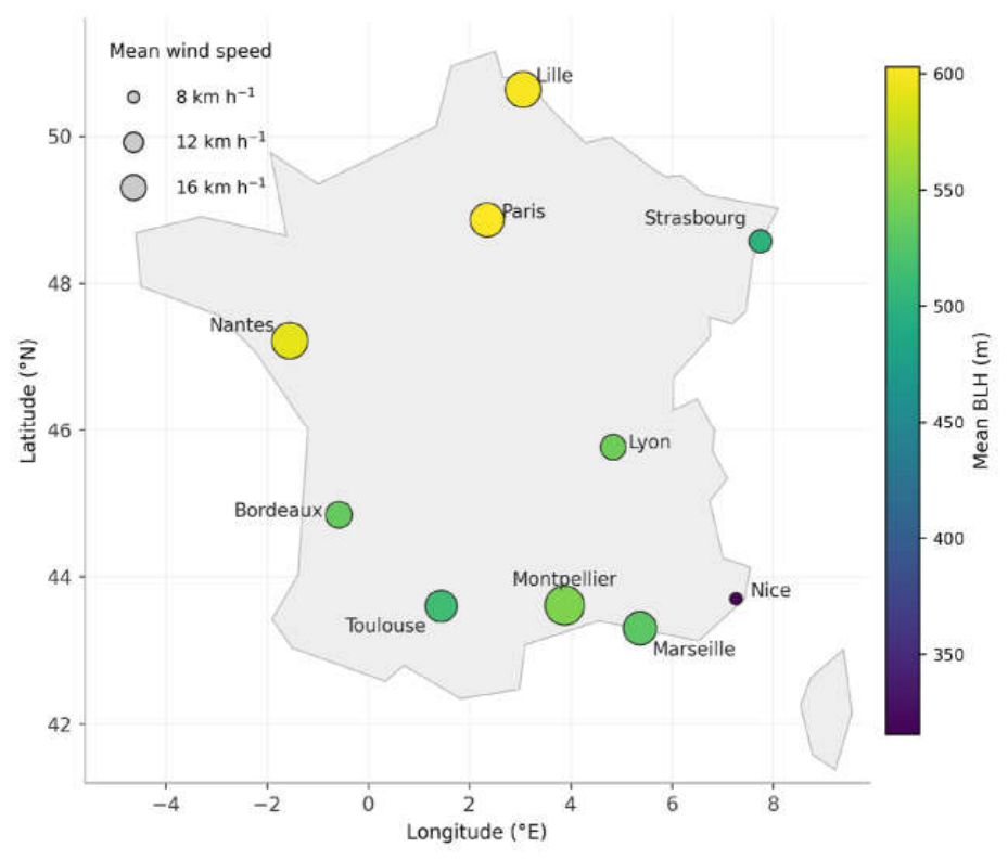
Figure 2.
The bivariate macro-pattern: Pearson correlation of each surface meteorological predictor with each pollutant, for every city (pooled daily levels). For the primary species (NO₂, PM₁₀, PM₂.₅) boundary-layer height and wind speed correlations are negative and pressure correlations are positive in almost every city. For O₃ the pattern reverses, with boundary-layer height and, above all, temperature strongly positive and relative humidity negative.
Figure 2.
The bivariate macro-pattern: Pearson correlation of each surface meteorological predictor with each pollutant, for every city (pooled daily levels). For the primary species (NO₂, PM₁₀, PM₂.₅) boundary-layer height and wind speed correlations are negative and pressure correlations are positive in almost every city. For O₃ the pattern reverses, with boundary-layer height and, above all, temperature strongly positive and relative humidity negative.
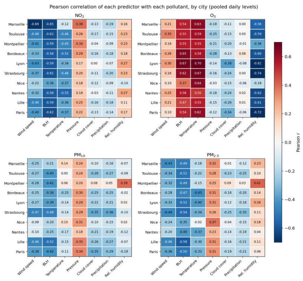
Figure 3.
The wind–boundary-layer collinearity that motivates the variance partitioning. (a) Daily 10 m wind speed against boundary-layer height at Paris (hexbin density plot, in which the plane is tiled with hexagons shaded by the number of days they contain; n = 2922 days) with the least-squares line. The two covary strongly (r = 0.72). (b) Pearson r(wind, BLH) for each city in the pooled daily frame (blue bars) and on deseasonalized monthly anomalies (orange bars). Dashed lines mark the ten-city means, 0.70 and 0.81.
Figure 3.
The wind–boundary-layer collinearity that motivates the variance partitioning. (a) Daily 10 m wind speed against boundary-layer height at Paris (hexbin density plot, in which the plane is tiled with hexagons shaded by the number of days they contain; n = 2922 days) with the least-squares line. The two covary strongly (r = 0.72). (b) Pearson r(wind, BLH) for each city in the pooled daily frame (blue bars) and on deseasonalized monthly anomalies (orange bars). Dashed lines mark the ten-city means, 0.70 and 0.81.
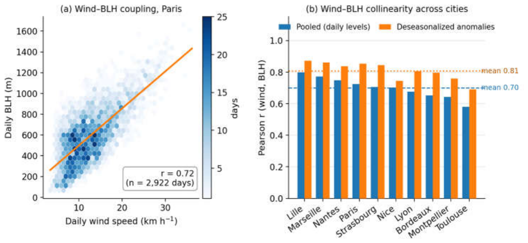
Figure 4.
Semi-partial R² as the unique-variance metric under wind–boundary-layer collinearity (schematic). (a) The variance of a pollutant partitioned between the two collinear drivers: sr²(wind) and sr²(BLH) are the variances unique to each (the non-overlapping crescents), while the shared wind–BLH variance (the overlap, reflecting r ≈ 0.70) is assigned to neither. The remainder is other predictors and unexplained variance. (b) The three metrics treat that shared variance differently (see text). Proportions are illustrative.
Figure 4.
Semi-partial R² as the unique-variance metric under wind–boundary-layer collinearity (schematic). (a) The variance of a pollutant partitioned between the two collinear drivers: sr²(wind) and sr²(BLH) are the variances unique to each (the non-overlapping crescents), while the shared wind–BLH variance (the overlap, reflecting r ≈ 0.70) is assigned to neither. The remainder is other predictors and unexplained variance. (b) The three metrics treat that shared variance differently (see text). Proportions are illustrative.
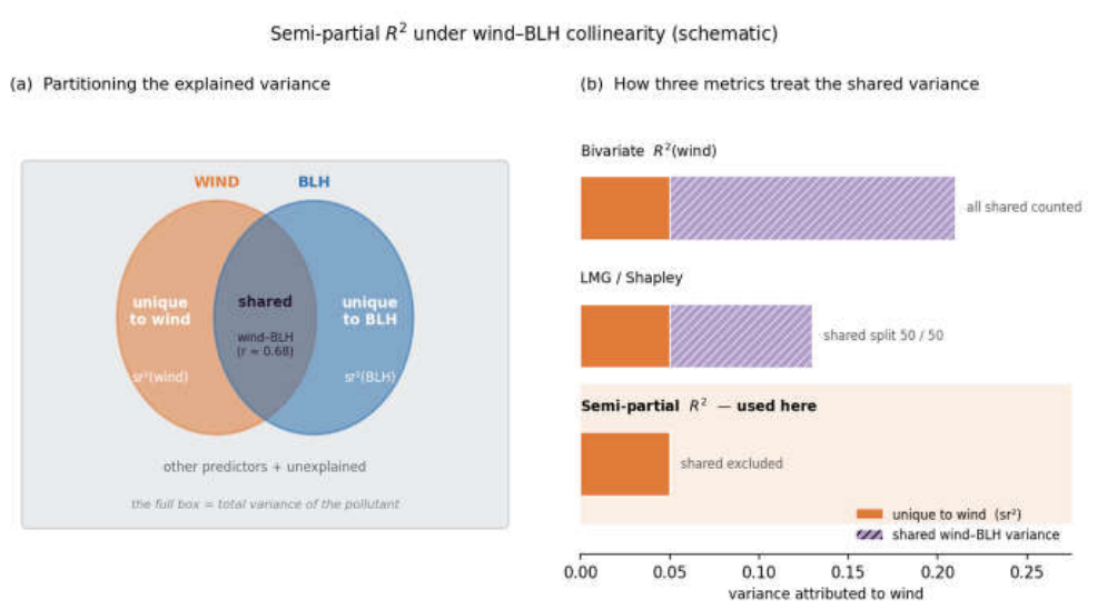
Figure 5.
Intrinsic persistence φ(Δ), the lag-1 autocorrelation of the deseasonalized series (month-by-hour climatology), against the aggregation window Δ, computed from the hourly record for the two reference cities, Marseille (left) and Lyon (right), for the four pollutants. Filled circles mark the crossover Δ* where φ = 0.5. The crossover orders the four species by atmospheric lifetime and sets the daily window as the finest resolution that retains weather-driven coherence. The rise of the NO₂ curve beyond about ten days is residual low-frequency structure that a month-by-hour climatology does not remove.
Figure 5.
Intrinsic persistence φ(Δ), the lag-1 autocorrelation of the deseasonalized series (month-by-hour climatology), against the aggregation window Δ, computed from the hourly record for the two reference cities, Marseille (left) and Lyon (right), for the four pollutants. Filled circles mark the crossover Δ* where φ = 0.5. The crossover orders the four species by atmospheric lifetime and sets the daily window as the finest resolution that retains weather-driven coherence. The rise of the NO₂ curve beyond about ten days is residual low-frequency structure that a month-by-hour climatology does not remove.
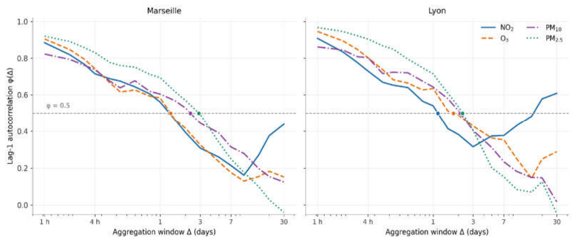
Figure 6.
The central result in the pooled frame: mean unique variance (semi-partial R²) of wind speed and boundary-layer height for each pollutant, across the ten cities (seven-predictor model). Error bars are the inter-city standard deviation.
Figure 6.
The central result in the pooled frame: mean unique variance (semi-partial R²) of wind speed and boundary-layer height for each pollutant, across the ten cities (seven-predictor model). Error bars are the inter-city standard deviation.
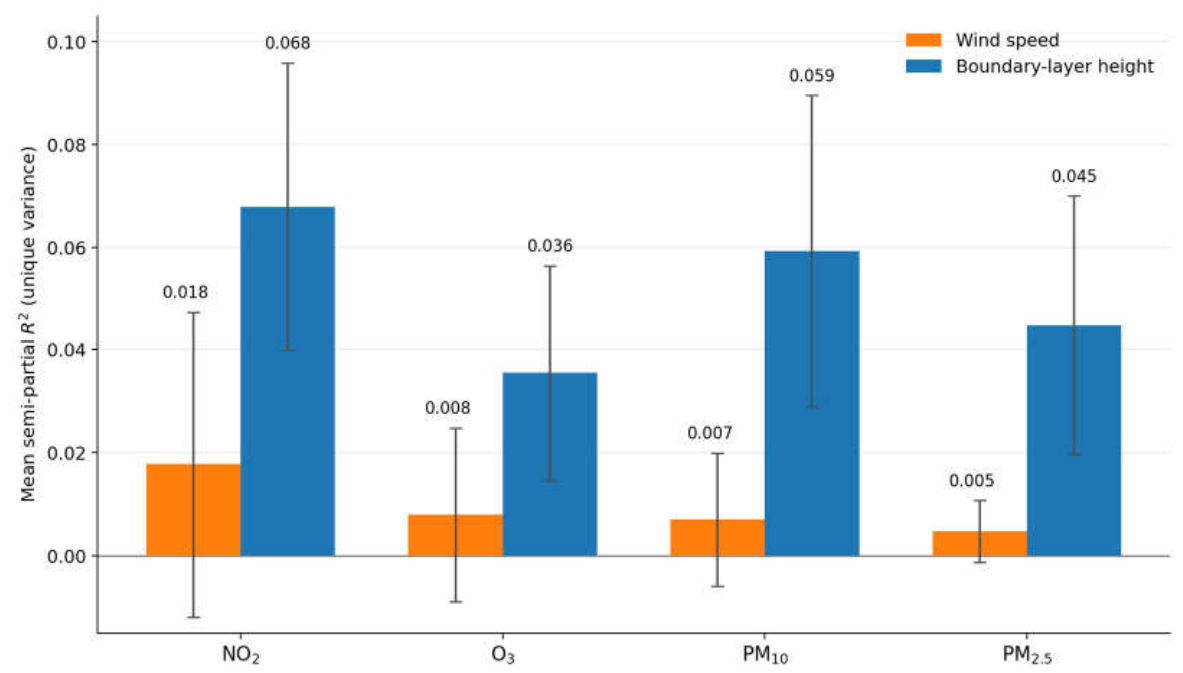
Figure 7.
Unique variance (semi-partial R²) of wind and BLH for each pollutant under the four analytical frames: pooled levels, season-stratified levels, deseasonalized monthly anomalies, and deseasonalized anomalies with the multi-year decline removed (mean over ten cities, seven-predictor model). Error bars are the inter-city standard deviation.
Figure 7.
Unique variance (semi-partial R²) of wind and BLH for each pollutant under the four analytical frames: pooled levels, season-stratified levels, deseasonalized monthly anomalies, and deseasonalized anomalies with the multi-year decline removed (mean over ten cities, seven-predictor model). Error bars are the inter-city standard deviation.
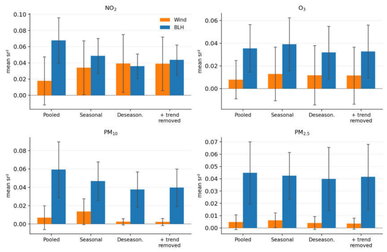
Figure 8.
Unique variance of wind speed versus the wind-direction Fourier block (sin θ, cos θ, sin 2θ, cos 2θ) for each pollutant (pooled frame, mean over ten cities). Both terms are added last in the seven-predictor model augmented with the direction block, so the comparison is like-for-like. Error bars are the inter-city standard deviation.
Figure 8.
Unique variance of wind speed versus the wind-direction Fourier block (sin θ, cos θ, sin 2θ, cos 2θ) for each pollutant (pooled frame, mean over ten cities). Both terms are added last in the seven-predictor model augmented with the direction block, so the comparison is like-for-like. Error bars are the inter-city standard deviation.
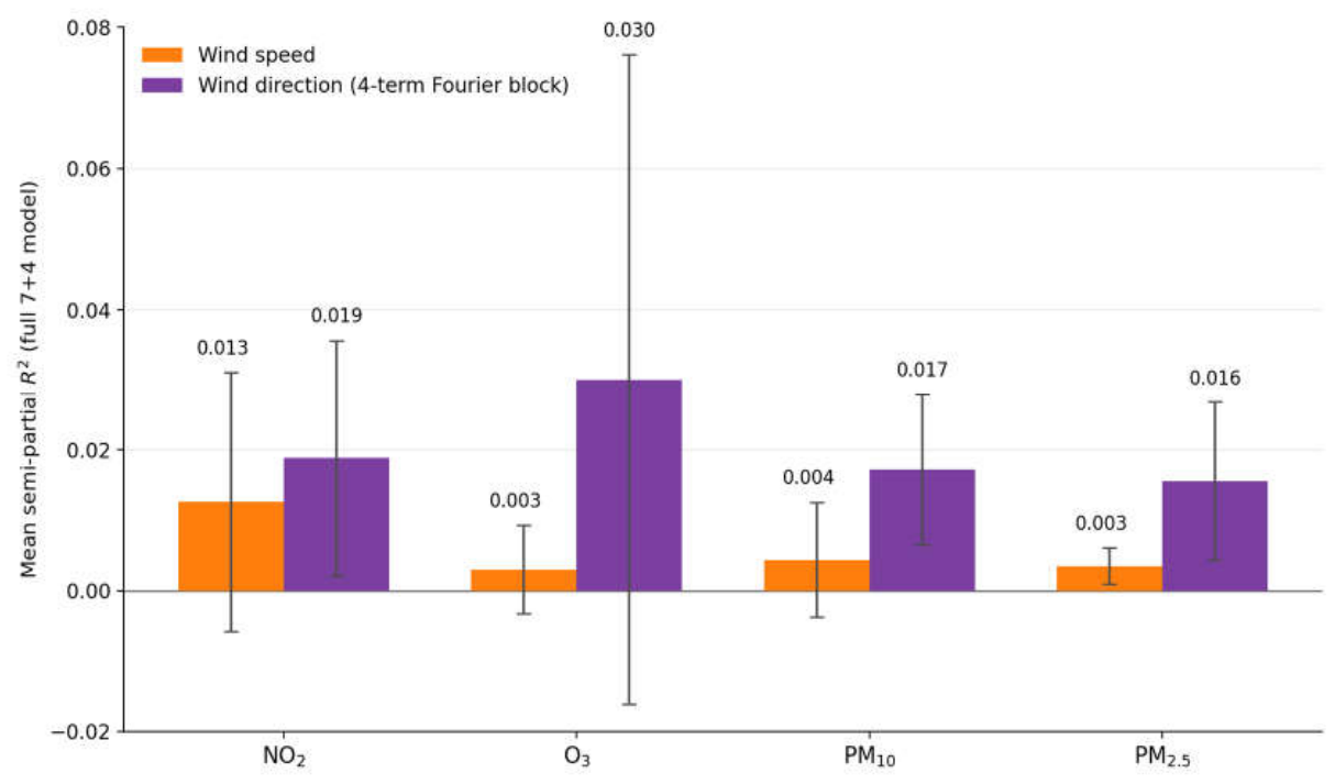
Figure 9.
Per-city decomposition of the NO₂ wind signal deseasonalized and with the calendar-year means removed: unique variance (semi-partial R²) of wind speed and of boundary-layer height in the seven-predictor model, one row per city, with the ten-city mean at the foot. The ≈ sign marks the five cities whose wind and BLH bootstrap confidence intervals overlap (Table S3), and the ten-city mean, whose two intervals also overlap.
Figure 9.
Per-city decomposition of the NO₂ wind signal deseasonalized and with the calendar-year means removed: unique variance (semi-partial R²) of wind speed and of boundary-layer height in the seven-predictor model, one row per city, with the ten-city mean at the foot. The ≈ sign marks the five cities whose wind and BLH bootstrap confidence intervals overlap (Table S3), and the ten-city mean, whose two intervals also overlap.
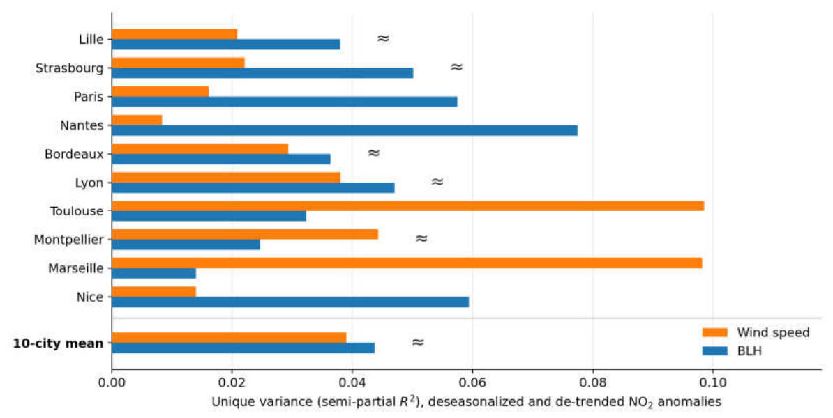
Figure 10.
Urban-meteorological typology from the fourth-rung NO₂ decomposition, deseasonalized and with the calendar-year means removed: wind unique variance (x-axis) against BLH unique variance (y-axis), one point per city, coloured by type.
Figure 10.
Urban-meteorological typology from the fourth-rung NO₂ decomposition, deseasonalized and with the calendar-year means removed: wind unique variance (x-axis) against BLH unique variance (y-axis), one point per city, coloured by type.
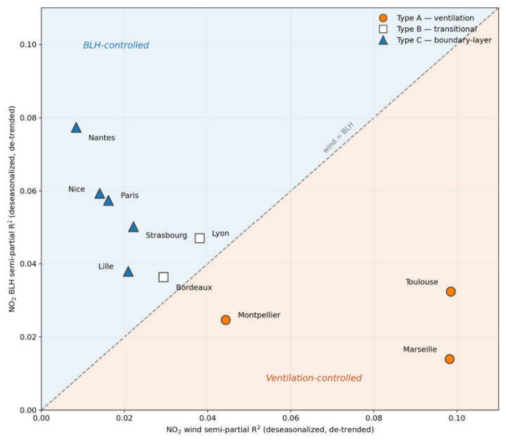

Table 1.
The ten study cities: climate class, topographic setting, regional wind regime and number of urban-background stations used. Köppen–Geiger climate classification. The regional wind regime column indicates the presence of a recurrent, near-unidirectional ventilating wind system.
Table 1.
The ten study cities: climate class, topographic setting, regional wind regime and number of urban-background stations used. Köppen–Geiger climate classification. The regional wind regime column indicates the presence of a recurrent, near-unidirectional ventilating wind system.
| City | Köppen climate | Topographic setting | Regional wind regime | Urban-background stations |
|---|---|---|---|---|
| Lille | Cfb | Flat plain | None dominant | 1 (see reservation) |
| Strasbourg | Cfb/Dfb | Rhine plain, sheltered | None dominant | 2–3 |
| Paris | Cfb | Flat basin | None dominant | 7 |
| Nantes | Cfb | Loire estuary | None dominant | 1 |
| Bordeaux | Cfb/Csa | Garonne estuary | None dominant | 1 |
| Lyon | Cfb/Csa | Rhône–Saône valley | Valley channelling | 2–3 |
| Toulouse | Cfb/Csa | Garonne plain | Autan, Tramontane | 1 |
| Montpellier | Csa | Mediterranean plain | Tramontane (moderate) | 1 |
| Marseille | Csa | Mediterranean hills | Mistral | 2–3 |
| Nice | Csa | Sheltered bay, Alps | None dominant | 1 |
Table 2.
2018–2025 descriptive statistics (mean ± SD), computed from the empirical record at urban-background stations. V̄ 10 m wind speed; T̄ 2 m temperature; P̄ surface pressure; BLH boundary-layer height (ERA5). Pressure is a period mean at the ERA5 surface height of the grid cell, which explains the differences between cities.
Table 2.
2018–2025 descriptive statistics (mean ± SD), computed from the empirical record at urban-background stations. V̄ 10 m wind speed; T̄ 2 m temperature; P̄ surface pressure; BLH boundary-layer height (ERA5). Pressure is a period mean at the ERA5 surface height of the grid cell, which explains the differences between cities.
| City | V̄ (km h⁻¹) | T̄ (°C) | P̄ (hPa) | BLH (m) | PM₁₀ (µg m⁻³) | PM₂.₅ (µg m⁻³) | NO₂ (µg m⁻³) | O₃ (µg m⁻³) |
|---|---|---|---|---|---|---|---|---|
| Lille | 13.7 ± 5.8 | 11.8 ± 5.9 | 1013.5 | 600 ± 272 | 20.1 ± 11.4 | 13.0 ± 9.1 | 19.8 ± 11.7 | 49.6 ± 20.7 |
| Strasbourg | 8.5 ± 4.6 | 12.1 ± 7.3 | 990.5 | 496 ± 266 | 17.4 ± 9.6 | 11.3 ± 7.9 | 19.0 ± 9.2 | 47.7 ± 24.8 |
| Paris | 12.9 ± 5.5 | 12.4 ± 6.5 | 1004.0 | 603 ± 269 | 18.1 ± 8.7 | 11.5 ± 7.4 | 24.1 ± 11.6 | 48.5 ± 20.8 |
| Nantes | 13.9 ± 5.6 | 13.2 ± 5.9 | 1012.1 | 593 ± 254 | 15.1 ± 7.4 | 9.2 ± 6.2 | 10.6 ± 6.6 | 56.7 ± 19.2 |
| Bordeaux | 10.2 ± 3.9 | 14.6 ± 6.4 | 1011.8 | 535 ± 242 | 15.1 ± 8.7 | 9.7 ± 7.6 | 12.9 ± 8.1 | 53.4 ± 20.1 |
| Lyon | 9.8 ± 4.8 | 13.1 ± 7.3 | 975.8 | 540 ± 273 | 17.4 ± 10.8 | 11.0 ± 8.6 | 20.5 ± 11.5 | 49.6 ± 24.9 |
| Toulouse | 12.0 ± 5.6 | 14.7 ± 6.8 | 992.7 | 514 ± 235 | 14.8 ± 7.6 | 8.7 ± 5.5 | 13.7 ± 8.5 | 57.1 ± 21.5 |
| Montpellier | 15.3 ± 6.6 | 16.0 ± 5.8 | 1009.1 | 547 ± 312 | 15.2 ± 8.4 | 8.5 ± 5.7 | 15.5 ± 8.9 | 57.9 ± 20.3 |
| Marseille | 12.6 ± 6.6 | 15.9 ± 7.1 | 997.6 | 531 ± 277 | 19.2 ± 9.5 | 9.9 ± 5.7 | 26.7 ± 11.9 | 57.0 ± 22.2 |
| Nice | 6.8 ± 2.9 | 15.0 ± 6.1 | 967.2 | 316 ± 161 | 18.7 ± 8.1 | 10.2 ± 4.8 | 25.4 ± 9.3 | 50.8 ± 23.0 |
Table 3.
Typology of the ten cities by the NO₂ wind/BLH balance on anomalies deseasonalized and with the calendar-year means removed.
Table 3.
Typology of the ten cities by the NO₂ wind/BLH balance on anomalies deseasonalized and with the calendar-year means removed.
| City | Type | NO₂ wind sr² | NO₂ BLH sr² | Dominant | Setting / regime |
|---|---|---|---|---|---|
| Marseille | A, ventilation | 0.098 | 0.014 | Wind | Mistral |
| Toulouse | A, ventilation | 0.099 | 0.032 | Wind | Autan / Tramontane |
| Montpellier | A, ventilation | 0.044 | 0.025 | Wind (CI overlap) | Tramontane (weaker) |
| Bordeaux | B, transitional | 0.029 | 0.037 | ≈ equal | Oceanic plain |
| Lyon | B, transitional | 0.038 | 0.047 | ≈ equal | Rhône valley |
| Strasbourg | C, boundary layer | 0.022 | 0.050 | BLH (CI overlap) | Sheltered (Rhine plain) |
| Nice | C, boundary layer | 0.014 | 0.059 | BLH | Coastal / Alps |
| Nantes | C, boundary layer | 0.008 | 0.077 | BLH | Oceanic plain |
| Lille | C, boundary layer | 0.021 | 0.038 | BLH (CI overlap) | Flat plain (data res.) |
| Paris | C, boundary layer | 0.016 | 0.057 | BLH | Basin |
Disclaimer/Publisher’s Note: The statements, opinions and data contained in all publications are solely those of the individual author(s) and contributor(s) and not of MDPI and/or the editor(s). MDPI and/or the editor(s) disclaim responsibility for any injury to people or property resulting from any ideas, methods, instructions or products referred to in the content. |
© 2026 by the authors. Licensee MDPI, Basel, Switzerland. This article is an open access article distributed under the terms and conditions of the Creative Commons Attribution (CC BY) license (http://creativecommons.org/licenses/by/4.0/).
Copyright: This open access article is published under a Creative Commons CC BY 4.0 license, which permit the free download, distribution, and reuse, provided that the author and preprint are cited in any reuse.