

Submitted:
25 September 2026
Posted:
29 September 2026
You are already at the latest version
Abstract
Exergy analysis is a powerful tool for identifying and quantifying irreversibilities in energy systems, yet its practical application is often hindered by the need to perform iterative calculations of enthalpy and entropy variations for real streams. In this paper, we generalize the concept of thermodynamic overall temperature, defined as T_overall = Δh/Δs between two thermodynamic states. This quantity extends the so-called entropic temperature to characterize any fluid transformation, whether isobaric or involving pressure drops, with or without transfer of work. For an isobaric flow of non-compressible fluid or ideal gas, T_overall reduces to the well-known logarithmic mean temperature. For real stream with pressure variation, its value is expressed in a simple, explicit, and general form, as a function of both the logarithmic mean temperature evaluated at the discharge pressure and an isentropic dissipation factor. This formulation enables the exergy of any real stream to be written in the simple Carnot-like form \( \dot{E}_y = [1 - T_a / \tilde{T}]\dot{Y} \), where\( \dot{Y} \) is the flow energy rate. Based on this unified formulation, we derive explicit expressions for exergy losses and efficiencies for key components, including compressors, turbines, expansion valves, heat exchangers (with and without phase change) and piping sections. Three summary tables synthesize the models according to component type and fluid streams. An extensive validation of models is carried out using the ADVENS Props library for various fluids including water, CO2, propane and ammonia. The maximum relative errors remain exceptionally low: below 0.22% for compressors (mean 0.05%), 0.45% for turbines (mean 0.08%), 0.02% for evaporators (mean 0.01%), and 2.2% for condensers (mean 0.20%), with the valve exhibiting a nearly zero error (machine precision). These results confirm the accuracy and robustness of the explicit formulation for engineering purposes. The proposed framework bridges the gap between classical pinch analysis and real-flow simulation, and the approach is illustrated on typical high-temperature and low-temperature network configurations.
Keywords:
exergy analysis
; thermodynamic overall temperature
; logarithmic mean temperature
; isentropic efficiency
; heat pumps and ORC components
; irreversibility
; energy systems
; pinch analysis
; energy efficiency
1. Introduction
The transition toward sustainable energy systems requires a paradigm shift from mere energy conservation to a more rational use of energy resources. While the first law of thermodynamics accounts for the quantity of energy, its coupling with the second law introduces the notion of energy quality through exergy, defined as the maximum useful work that a system can provide when it reaches equilibrium with its environment. The genesis of this exergy concept has its roots in “usable energy” by Gouy (1889) [2] and Darrieus (1931) [3], “availability” by Keenan (1932, 1951) [4,5], up to the official introduction of the term “exergy” by Z. Rant in 1956 [6]. Exergy analysis today becomes a powerful method for identifying and quantifying irreversibilities in energy conversion systems, providing a common basis for comparing different energy vectors such as heat, work, and electricity [7,8,9].
Beyond the theoretical formulations of exergy, engineering of energy systems and heating/cooling processes relies on a precise and differential taxonomy of exergy losses (exergy efficiency). Borel & Favrat (2010) [8] propose a fundamental decomposition of total exergy losses () into two distinct physical categories [10]:
where represents dissipation losses (pressure drops, internal fluid friction, viscous effects) and represents heat transfer losses (irreversibilities related to temperature differences between the fluid and hot or cold sources) [8]. These losses, developed in the reference work by Favrat & Kane [10], are functions of the temperature levels of fluids and sources.
One of the main obstacles to the generalized application of exergy analysis in industrial practice is the need to apply implicit co-enthalpy functions to simultaneously calculate enthalpy and entropy variations of real energy streams. The primary objective of this article is to use an explicit formulation of the exergy of any real fluids that is expressed in the simple Carnot form [10]:
where is the flow energy and represents the thermodynamic mean temperature that we call here simply the “overall temperature”. It is defined according to the following expression:
For a thermodynamic process at constant pressure (), the thermodynamic mean temperature corresponds simply to the entropic mean temperature widely used in thermochemistry, for applications where dissipations are neglected [11]:
where represents the amount of heat transferred. Based on these definitions, we explore here the relationships between exergy losses and temperature levels of hot and cold streams of any thermodynamic system and then establish explicit expressions for exergy losses and efficiencies for the most common key components — compressors, pumps, turbines, expansion valves and heat exchangers (with and without phase change).
1.1. Thermodynamic Definitions of Mean Temperature
The idea of applying thermodynamic mean temperature to characterize real transformations (e.g. with irreversibilities) has progressively emerged in literature.
As early as 1991, Marquet (1991) [12] laid the very first stone of the idea of an intrinsic thermodynamic temperature of a fluid stream to estimate the totality of transformation irreversibilities. Building on the original works of Maxwell (1871) [13] and Gibbs (1873) [14], he rigorously adopted the notion of available enthalpy using the thermodynamic mean temperature to model the potential work energy carried by a fluid stream.
In 1995, Staine (1995) [15] introduced a pseudo-temperature for streams with dissipation, allowing the extension of pinch analysis to pseudo-Carnot factors. This pioneering work opened the way to the integration of pressure drops in the exergy analysis of hot and cold streams of heat exchangers, as well as to the consideration of dissipations or friction in the analysis of flows in compression or expansion in mechanical components. Staine’s formulation nevertheless relied on an implicit definition of pseudo-temperature, requiring successive iterations between the heat exchanger thermal balance and pressure drops, particularly in two-phase zones or during complex thermal couplings. This approach, although foundational, complicated calculations and made direct integration into network simulation tools difficult.
Ziegler (1998) [16] brought a fundamental clarification by distinguishing the different temperature averages used in heat exchangers. He demonstrated that the logarithmic mean temperature difference (LMTD) and the entropic mean temperature measure fundamentally different aspects: the entropic temperature difference is a measure of efficiency, while the logarithmic temperature difference is a measure of the exchanger cost [16].
The thermodynamic mean temperature (or entropic temperature) is defined by , where Q is the heat exchanged and the entropy variation [16]. Ziegler demonstrates that in most technical applications, these quantities are very close (within 10%) and can be approximated by the simple difference of arithmetic means. This duality between cost and efficiency is at the heart of exergoeconomic optimization, as it directly links investment cost (via the exchange surface determined by the LMTD) to operating cost (via exergy destruction determined by the entropic temperature) [16].
Schiffmann and Favrat (2011) [17] made a significant contribution by demonstrating that for small turbomachines, where heat transfer is no longer negligible, the isentropic efficiency must be corrected to account for heat losses. They introduced a generalized entropic temperature defined by:
where represents internal friction losses and heat transfer. This entropic temperature is identical to the Gibbs temperature for processes with work-energy exchange, and allowed separating internal friction losses from parasitic heat transfers, enabling more precise optimization of the compressor and its cooling system. These works are based on the fundamental thermodynamic equations provided by Borel & Favrat [10].
Khennich et al. (2014) [18] used the equivalent temperature to construct a Carnot factor vs. enthalpy variation diagram () for exergy analysis of ejector cycles. They proposed replacing real adiabatic processes (compression, expansion, throttling) by a combination of an isentropic step (where and ) followed by an isobaric step (where is calculated by ) [18]. This approach visualizes exergy losses as rectangular areas on the diagram, facilitating the identification of the most irreversible components.
The entropic temperature has proven particularly useful for the analysis of complex thermochemical systems. Meunier et al. (1996) [11] as well as Meunier et al. (1998) [19] applied second law analysis to compare liquid absorption, solid adsorption, and chemical reaction systems. They introduced the concept of entropic temperatures () as logarithmic mean exchange temperatures, allowing real systems with irreversibilities to be transformed into equivalent endoreversible Carnot cycles.
The entropic temperature associated with heat exchange for each phase of the sorbent is defined by:
where is the temperature of the sorbent, which varies in time or space. This approach facilitated the calculation of COP and exergy efficiency. Meunier et al. (1996) [11] identified the dominant sources of exergy destruction: for liquid absorption, the solution expansion corresponds to more losses, while for solid sorption, losses due to heat devaluation (temperature differences between the reactor and sources) are dominant, representing up to 98% of entropy production in certain cycles.
Castaing-Lasvignottes and Neveu (1998) [20] extended this concept to solid/gas resorption systems, demonstrating that the quantity associated with mass transfer between reactors plays a role strictly analogous to mechanical work in conventional vapor compression cycles. Using entropic temperatures, they transformed a real cycle with internal irreversibilities into an equivalent reversible Carnot cycle [20]. Their analysis showed that the main source of entropy production comes from thermal coupling between reactors and sources, as well as gas transfer (superheating and desuperheating).
The decisive conceptual leap toward a more general definition was accomplished by Neveu (2002) [21] in his Habilitation to Direct Research memoir. To overcome the limitations of analyses restricted to simple heat transfers, Neveu uses the concept of “equivalent Gibbs systems” based on Clausius’s law of equivalence of transformations [22] to model unsteady regimes and real components in flow.
To establish the rigor of this model, the author fundamentally relies on the foundational works of Prigogine (1962) [23] concerning the Thermodynamics of Irreversible Processes (TIP) and the local equilibrium hypothesis. However, Neveu brings a decisive modification: to characterize the energy of a fluid in continuous motion, he substitutes the internal energy flux used by Prigogine with the enthalpy flux. By cross-referencing this local microscopic approach with standardized macroscopic balances from engineering textbooks by Bejan (1982) [24] and Van Wylen (1973) [25], he ensures that the balances remain valid at the scale of industrial processes.
From this synthesis, Neveu defines an equivalent temperature associated with a dynamic fluid in flow, such as adiabatic compression or expansion in an open thermodynamic system. It is expressed by the ratio of specific enthalpy variation to entropy variation. Neveu thus establishes the foundational algebraic definition:
In his equivalent Gibbs systems method, Neveu shows that this quantity allows determining entropy production in bilinear form and deriving phenomenological laws relating matter, heat, and entropy fluxes [21].
For the classical ideal cases (perfect gas or incompressible liquid at constant pressure), this equivalent temperature reduces exactly to the logarithmic mean temperature:
In his equivalent Gibbs systems method, Neveu showed that this quantity allows determining entropy production in bilinear form and deriving phenomenological laws relating matter, heat, and entropy fluxes [21].
Canivet (2017) [26] further developed this work by redefining the “hot” or “cold” character of a fluid in flow using its pseudo-temperature , where and relate to the environment [26]. He distinguishes “standard” cases from non-standard cases where becomes negative, changing the direction of exergy propagation. To justify this singularity and prove that the equation has fundamental physical meaning, Canivet draws on the statistical physics work of Leff (1996, 1999, 2007) [27], who conceives entropy not as disorder but as a measure of the dilution of energy within the degrees of freedom of a system [27]. By intersecting Neveu [21] and Leff [27], Canivet proves that a negative pseudo-temperature from the equation simply characterizes a state of energy density deficit of the fluid compared to the environment [26].
Canivet [26] also proposed graphical representations (exergography) using geometric areas (or bricks) and introduced the Joule-x as a unit dedicated to exergy. This work provided the conceptual framework to integrate pressure drops and real fluid behavior into a visual and intuitive exergy analysis.
In the field of district heating, various studies have shown that the exergy performance of a network can be determined based on a relation that directly links the logarithmic mean temperature to exergy losses. Poredoš et al. (2019) [28] used the logarithmic mean temperature to calculate exergy destruction in domestic hot water boosters, comparing different technologies (electric resistance, gas boiler, heat pump) [28]. They demonstrated that for ultra-low temperature networks, the heat pump booster offers the highest exergy efficiency and the lowest CO2 emissions.
The doctoral work of Adihou (2022) [29] extended these mean temperature concepts to the exergy modeling and optimization of district heating networks. Yolaine developed explicit and simplified formulations to calculate exergy losses of the distribution network as a function of the arithmetic mean temperature of the network , the supply and return temperature levels at substations, supply and return at the production plant, and total pressure drops across the entire network :
First term: Thermal exergy losses (related to temperature differences)
Second term: Exergy losses by viscous dissipation (related to pressure drops)
Two components can be distinguished: internal thermal exergy losses (related to temperature differences) and internal viscous exergy losses (related to viscous friction). She shows that heat devaluation due to temperature differences between supply and return flows is a major source of irreversibility [29]. Her methodology was validated on real networks using the ADVENS software [1] , which implements the quantized network method for thermo-hydraulic simulation [29].
Sharew et al. (2024) [30] combined exergy analysis and pinch analysis to optimize a steam turbine cogeneration plant. They calculated the exergy of a heat flow using a relation that directly links the logarithmic mean temperature to exergy destruction [30]. Their results showed that high-pressure heat exchangers can represent up to 31% of total exergy losses, and that strategic integration of heat pumps above the pinch point can enable energy savings of up to 83 MW [30].
1.2. Physical Foundations of Mean Temperature
In most practical cases for quantifying losses and irreversibilities of a thermodynamic open process between two states (1 and 2), the Gibbs relation can be used to calculate the rate of enthalpy change of the system relative to the entropy change . For a process at constant pressure (or constant volume), this rate corresponds to the entropic temperature at constant pressure, defined above from the following fundamental equations of Maxwell:
The fundamental distinction between caloric and entropic temperatures in non-equilibrium steady states (thermally non-homogeneous) is demonstrated by Criado-Sancho et al. (2016) [31]. They provide the physical justification for using entropic temperature (based on ) as the reference quantity for modeling real thermal couplings in a non-homogeneous closed system [31]. This entropic temperature, defined from the fundamental relation of thermodynamics, is considered the appropriate variable for characterizing irreversible processes, rather than the caloric temperature defined from the equation of state.
Yang et al. (2016) [32] introduced the concept of integration temperature difference , defined as the area bounded by the temperature-heat curves divided by the total heat energy transferred. This integral parameter, analogous to the entropic temperature difference or the logarithmic temperature difference, captures the entire heat transfer path, including superheating and phase change zones [32]. Their experimental validation with 52 thermocouples along an ORC evaporator demonstrated a linear relationship between and the entropy generation number .
Based on detailed modeling of a counter-current heat exchanger, Dong and Du (2021) [33] established the equation link between local heat transfer phenomena and entropy creation to analytically solve temperature profiles. They confirmed that the logarithmic mean temperature naturally arises from differential equations, and showed that local entropy generation is a bracket function of the local temperature ratio [33]. Their results illustrate the principle of equipartition of entropy generation: for a given heat exchange, the configuration that minimizes total entropy generation is the one with the most uniform local production [33]. This finding justifies the use of the logarithmic temperature difference to represent and illustrate the degradation state of hot and cold flows in a heat exchanger.
Allahverdyan et al. (2022) [34] address the rigorous thermodynamic definition of a mean temperature. Drawing on the statistical physics of Landau and Lifshitz (1980) [35] and the works of Casas-Vazquez and Jou (2003) [36] on open problems of non-equilibrium temperature, they postulate that the use of purely mathematical averages (arithmetic or geometric) is physically incorrect. They demonstrate that the true mean temperature of a system with energy transfer must lie between two extreme limits: a lower limit (perfectly reversible system where entropy is conserved) and an upper limit (totally irreversible system where energy is conserved):
Its value is determined by its energy (U or H) and entropy (S) via Lambert’s W function:
For example, for two initial gas systems at temperatures and , the thermodynamic mean temperature is expressed by the following relation:
where is the Lambert W function, defined as the solution to the equation [34].
This demonstration based on statistical physics proves that the evaluation of a global thermal state is fundamentally driven by the Energy/Entropy pair. These results based on statistical physics, requiring primarily a solution of the Lambert equation, validate a posteriori the relevance of formulating the thermodynamic mean temperature to characterize the degradation state of a fluid in non-equilibrium motion.
1.3. New Approach of Thermodynamic Mean Temperature
All these works converge toward the need to find a simple expression for the thermodynamic global temperature capable of capturing in the same quantity both thermal irreversibilities of heat transfer and mechanical dissipations (pressure drops). This allows unifying the definition and characterizing the level or degree of energy transformation of a real stream, whether at constant pressure or with dissipation, with or without work transfer. Favrat & Kane (2024) [10] formalized this concept under the name of overall temperature level of a flow and applied it to the basic components of heating and cooling systems. For any fluid evolving between two thermodynamic states 1 and 2, the thermodynamic mean temperature is expressed in a simple, explicit, and general form as a function of a logarithmic mean temperature calculated at constant discharge pressure and dissipation factor :
For an ideal stream without pressure variation, and corresponds to the logarithmic mean temperature between the two states 1 and 2. For a real stream with pressure variation, its value accounts for dissipations via the isentropic factor and the entropic temperature (or logarithmic mean temperature which ) is calculated at the final discharge pressure . The quantity capture the thermal irreversibilites derived from heating (and/or cooling) and the quantity is by definition known for any type of stream. For a compression flow, represents the isentropic compression efficiency and for an expansion flow in a turbine, it represents the inverse of the isentropic expansion efficiency . This concept of thermodynamic temperature is also extended to flows with phase change by dividing the flow into three zones (superheat, two-phase, subcooling).
In the present article, we take up and develop this concept of “thermodynamic mean temperature” to make it a systematic tool covering all components of energy systems. We will:
- 1.
- Model simply the flow exergy of any real stream using the Carnot factor relative to the overall temperature:
- 2.
- Formulate explicitly the exergy losses and efficiencies for compressors, turbines, valves, heat exchangers, pipes and others
- 3.
- Synthesize these results in a summary table allowing distinction of all performance parameters
- 4.
We introduce a more general definition of the hot or cold character of a real fluid in flow by considering its exergy level, characterized not only by its enthalpy variation and dissipation factor but also by its temperature level corresponding to the logarithmic mean temperature.
2. Modelling Streams With or Without Change in Pressure
Many thermodynamic processes are open systems that can be operated autonomously with flowrates or energy conversion that vary automatically to respond to a sudden change in heating or cooling demand. In this article, we’re studying the operation of an established system which has reached a stable state called steady state (in nominal or partial load), i.e. with flowrate and/or heatrate which remain constant. The thermodynamic parameters characterizing the behavior of the system are in this case time invariant.
2.1. Overall Temperature of a Stream at Constant Pressure
As mentioned above, the Gibbs relation of an open process between two states (1 and 2) can be used to calculate the rate of enthalpy change relative to the entropy change . Figure 1x illustrates the T-s diagram for calculating this quantity at constant pressure.
The following equations can thus be defined:
The combination of these two equations allows to establish the following relations:
where function is identified as the logarithmic mean temperature between state 1 and state 2, it derived from the entropic temperature at constant pressure. The logarithmic mean temperature of two different values is well known in Thermodynamics. It generally characterizes the temperature level at which energy and entropy exchanges occur in an ideal fluid stream (i.e., at constant pressure). For a given temperature difference between two states (temperature glides, ), its value is always less than or equal to the arithmetic mean temperature . Figure 2 illustrates the dimensionless glide values comparison between the average temperature and the logarithmic mean temperature .
Generated for a cold reference temperature °C, this figure plots the dimensionless ratio against the dimensionless temperature glide (where is the arithmetic mean). The dashed line is provided as a reference representing perfect equality between the two means.
In case of an isothermal transformation (zero glide), the logarithmic mean temperature coincide perfectly to the constant temperature .
In case of small temperature glides , the logarithmic mean temperature could be approximated by the average temperature.
In case of large temperature glides , the logarithmic mean temperature is always lower than the arithmetic average temperature . The gap between the two curves widens exponentially at extreme glides.
2.2. Overall Temperature of a Stream in Phase Change
In the case of a phase change fluid, for example in condensation at constant pressure, we can subdivide the process in different phases or zones: de-superheating gas zone (g), condensation bi-phasic zone (b) and subcooling liquid phase (l). Figure 3 shows the T-s diagram of a hot stream in condensation, where the three distinct zones are clearly identified: the superheated vapour region, the two-phase saturation region, and the subcooled liquid region.
The expression given in Equation (18) becomes:
Or, finally:
In which:
- and represent respectively the liquid and gas saturated entropy;
- represents the boiling (saturated) temperature corresponding to the working pressure;
- and correspond respectively to the logarithmic mean temperature value of the liquid and gas phases:
- is the enthalpy variation per unit mass of the flowing fluid in the subcooling zone;
- is the enthalpy variation per unit mass of the flowing fluid in the biphasic zone (it is important to note that: for this case of a fluid in condensation for a condensation where represents the enthalpy of vaporisation per unit mass and which is a positive value);
- is the enthalpy variation per unit mass of the flowing fluid in the de-superheating zone.
Equation (20) is also valid for the case of a fluid stream in evaporation and the enthalpy variation per unit mass of the flowing fluid in the biphasic zone is equal to the enthalpy of vaporisation .
This logarithmic mean temperature value (called here overall temperature level) of the fluid stream is based on the integration of the Gibbs relation between two states and at constant pressure. It allows to characterize irreversibilities in various processes and components by giving an explicit relation between enthalpy and entropy variations. Thus, the importance of the fluid temperature level on the energy performance can be demonstrated for the different basic unit processes.
2.3. Flow Energy/Exergy of Real Streams with Dissipation
We now extend the analysis to real streams where pressure drops and internal dissipations cannot be neglected. Such dissipations occur in most practical components: pipe sections or heat exchanger with friction, compressors with internal leakage and friction, turbines with irreversibilities, and expansion valves. To account for these effects, we consider the pressure variation between two states as an isentropic expansion followed by an isobaric step. Figure 4 illustrates the evolution of hot and cold streams with dissipations in the T-s diagram.
a- hot stream (1 → 2): For the calculation of the entropy difference of the hot stream as a function of the enthalpy variation, we first consider the isentropic expansion between state 1 and state 2s followed by the cooling process along the isobaric curve at pressure from state 2s to state 2 (i.e., ). The enthalpy decrease at the end of the cooling process can be expressed as a fraction of the total fluid transformation energy per unit mass:
Considering the relations in Equation (15) and Equation (16) between state 2s and state 2 at constant pressure , the entropy difference of the hot stream can be expressed as a function of the enthalpy difference and the logarithmic mean temperature at the outlet pressure:
where characterises the dissipation losses of the fluid in the hot stream, and is the logarithmic mean temperature calculated at the outlet pressure (equivalent to ).
We now introduce the thermodynamic overall temperature of the real hot stream, defined as:
This single quantity encapsulates both the temperature level and the internal dissipations of the stream. Substituting Equation (24) into Equation (23) yields the fundamental relation:
Consequently, the exergy received from the hot stream by a system (e.g., a heat exchanger) is expressed in the pure Carnot form:
where is the energy flow rate of the hot stream.
The exergy received by a system from a hot stream is thus a function of its thermodynamic overall temperature . The higher , the closer the Carnot factor is to unity, and the lower the exergy destruction.
b- cold stream (1’ → 2): A same analysis can be applied for a cold stream receiving heat from a system, also with pressure change and dissipations.
The entropy difference of the cold stream can be expressed as a function of the enthalpy difference and the logarithmic mean temperature at the outlet pressure:
with being the logarithmic mean temperature calculated at the outlet pressure (equivalent to ). The thermodynamic overall temperature of the cold stream is then defined as:
we obtain the analogous Carnot-form expression for the exergy provided by a system to the cold stream:
where .
The same conclusion can be drawn: the exergy provided by a system (e.g., a heat exchanger) to the cold stream is given by using a Carnot factor based on its thermodynamic overall temperature .
Such a formulation highlights that any real stream, regardless of its dissipation, can be characterized by a unique thermodynamic overall temperature for which, we can derive explicit expressions for the exergy performances of various specific components such as compressors, pumps, turbines, expansion valves, heat exchangers, and pipe sections. The thermodynamic overall temperature is systematically applied to model streams of each component.
2.4. Flow Energy/Exergy of a Cold Stream in Compression Process
2.4.1. Compression Process in Adiabatic Compressor
Figure 5 shows in a T-s diagram the compression process of a fluid in a compressor (K) considered adiabatic (i.e., without heat transfer with the outside). The non-isentropic nature of this compression suggests in practice the use of an internal isentropic efficiency to take into account the irreversibilities of internal heat transfer and dissipation. If the variations in the kinetic and potential energies of the fluid are neglected in relation to the work energy consumed by the compressor, the isentropic efficiency of the compression is then expressed by the following relation:
where quantities and respectively represent fluid enthalpy levels at the inlet and outlet of the compressor and would be the output enthalpy value if the transformation were ideal (i.e., without losses or irreversibilities: is the so-called isentropic enthalpy difference). The temperature at the compressor outlet for the real (non-reversible) compression is then higher than the corresponding to an ideal or reversible compression.
Enthalpy increase at the end of the compression process thus represents the dissipation energy per unit of mass and can be calculated as a percentage of the fluid transformation energy per unit of mass:
For the calculation of these dissipations as well as the difference in entropy of the system in function of the logarithmic mean temperature, we can consider the outlet isobaric (discharge) pressure curve from state 2s to state 2 (i.e., ). The following equations can thus be defined:
where represents the logarithmic mean temperature at discharge pressure corresponding to real and ideal expansion respectively. By combining the two previous equations, we can finally express this difference in entropy by the following simple relation:
Introducing the thermodynamic overall temperature of the compression process:
yields the fundamental relation:
Consequently, the exergy provided to the cold stream by the compressor is expressed in the pure Carnot form:
where is the energy flow rate received by the fluid.
The global exergy losses in the compressor, including external losses via the effectiveness (which accounts for heat losses to the environment), is:
and the exergy efficiency of the compressor is:
From these expressions of compressor losses and exergy efficiency, we can visualize the effect of the overall temperature on the exergy performance of a compressor. Figure 6 shows the specific exergy losses represented by and the exergy efficiency in function of this overall temperature.
The following can be learned:
For the same enthalpy difference and also the isentropic efficiency, it is better to operate a compressor with the highest possible temperature. Thus, the best choice of fluid for a compressor is the one characterized by a higher temperature level . For the same working fluid in a compressor, adiabatic compression is aimed at, i.e. with perfect thermal insulation from the external environment to obtain the best exergy efficiency. The expressions for the exergy loss and the exergy efficiency are better for an effectiveness equal to unity .
2.4.2. Pumping Process of an Non Compressible Fluid
A pump is the hydraulic component analogue to a compressor, but applied to a non-compressible fluid . The same reasoning in compression can be applied rigorously and the isentropic efficiency of the pump is defined as:
where the parameter represents the polytropic caloric factor for a non-compressible fluid evolution, more generally defined in Borel & Favrat [8] by for any real fluid.
Based on the compression exergy analysis described above for a compressor, the exergy services provided by pump to the stream is therefore:
where and is the thermodynamic mean temperature for the pump process, given in function of the logarithmic mean temperature at the outlet pressure and the isentropic efficiency of the pump :
For this non-compressible fluid in a pump, and the logarithmic mean temperature could be approximated by the average temperature between the inlet and outlet of the pump. The following equation can then be given for the pump:
and the exergy efficiency of the pump is:
2.5. Flow Energy/Exergy of a Hot Stream in Expansion Process
2.5.1. Expansion Process in Adiabatic Turbine
Figure 7 shows in a T-s diagram the expansion process of a fluid in a turbine (T) considered adiabatic (i.e., without heat transfer with the outside). Based on the same reasoning used for the compression, fluid dissipation losses in an adiabatic turbine expansion can be quantified using the isentropic efficiency of the turbine . The latter takes irreversibilities into account and can be expressed by the following relation, if we disregard the variations of kinetic and potential energies of the fluid in relation to the energy actually transformed into work:
where and respectively represent the enthalpy values of the fluid at the inlet and outlet of the turbine, and is the outlet enthalpy value if the transformation were ideal. Temperature at the outlet of a real expansion is then higher than the ideal expansion temperature .
The enthalpy increase represents the dissipation energy per unit of mass and can be calculated by:
or by the hatched area of the T-s diagram:
where is the logarithmic mean temperature at discharge pressure corresponding to real and ideal expansion respectively:
Combining the two previous equations, we obtain:
Introducing the thermodynamic overall temperature of the expansion process:
we find the fundamental expression of enthalpy/entropy relationship:
Note that the value of is necessarily negative given that the enthalpy of the fluid decreases during expansion while its entropy increases due to dissipation. The exergy received by the turbine from the hot stream is therefore expressed in the pure Carnot form:
where .
Considering that , where is the turbine effectiveness, the overall exergy losses and efficiency of the turbine become:
Figure 8 shows the effect of on the specific exergy losses and the exergy efficiency.
The same conclusion can be drawn: for the same enthalpy difference and isentropic efficiency, it is better to operate a turbine with the highest possible thermodynamic overall temperature . For the same working fluid, adiabatic expansion (perfect insulation, ) is aimed at to obtain the best exergy efficiency.
2.5.2. Expansion Process in a Valve
The expansion of a fluid or gas can also be carried out without producing mechanical energy by letting the fluid expand through a valve. Expansion valves are very often used in heating or cooling systems and more particularly in heat-pump cycles. Compared to a turbine, all the energy and exergy services received by the valve are totally destroyed, i.e. without any benefits being provided.
The isentropic efficiency of a valve characterizes the non-isenthalpic expansion due to a non-adiabatic expansion process (e.g. losses to the atmosphere). It is defined here as:
where and are the inlet and outlet enthalpies, and is the enthalpy after an isentropic expansion to the outlet pressure. Its value is very low compared to the isentropic efficiency of a turbine. For a perfectly insulated valve (adiabatic), the actual enthalpy difference is zero (), which corresponds to the classical isenthalpic (Joule-Thomson) expansion.
Based on the expansion exergy analysis described above for a turbine, the exergy services received by the valve from the hot stream (which is entirely destroyed, exergy efficiency equal to zero: ) is therefore:
where is the thermodynamic mean temperature for the expansion, given in function of the logarithmic mean temperature at the outlet pressure and the isentropic efficiency :
The following equation can then be given for the valve:
Or then again:
where is the isentropic enthalpy variation. This expression clearly separates the exergy losses due to external heat transfers from those due to internal dissipation .
Figure 9 shows the specific exergy losses based respectively on the enthalpy variation represented by and on the isentropic enthalpy variation represented by in function of the overall temperature level out of the valve .
From expression of an expansion valve exergy losses, the following can be learned:
In the case of an adiabatic expansion in a valve, i.e., with perfect thermal insulation thus avoiding external heat losses , the enthalpy variation of the fluid is equal to zero (isenthalpic expansion): This is the method widely used in industry to cool or even liquefy a gas by means of the Joule-Thomson expansion of a real gas. Equation (59) becomes:
In the case of an isenthalpic two-phase flow expansion in a valve (like an expansion valve in a heat-pump), the temperature at the outlet of the valve remains constant and corresponds to the saturated temperature of the working pressure at the evaporator: . The isentropic enthalpy variation can be given by:
So, for a biphasic expansion:
In the case of a perfect gas flow expansion in a valve, the temperature difference between the inlet and outlet of the valve is equal to zero for an isenthalpic expansion: . Based on the equation of state and the enthalpy variation of a perfect gas:
The integration becomes:
In the case of a liquid flow expansion in a valve, it can be considered that the specific volume per unit of mass does not change with temperature and that the temperature variation is very small: . The expression becomes:
The exergy losses for a liquid are higher at low temperatures than at high temperatures.
3. Summary Tables: Real Streams and Components
The previous sections have established a unified framework for expressing the exergy associated with any real fluid stream. The key result is the generalization of the Carnot form flow exergy, which allows any stream to be characterized by a unique and simple thermodynamic overall temperature:
where represents the logarithmic mean temperature calculated at the outlet pressure and the isentropic dissipation factor of the process which characterizes the internal irreversibilities. For isobaric processes, and , which reduces to the classical logarithmic mean temperature. The general exergy expression for any real stream is:
where is the flow energy carried by the stream and is the ambient temperature.
The increase or decrease of a fluid’s enthalpy can be achieved not only by heating or cooling (as in classical pinch analysis) but also by compression or expansion. A flow in compression is then a cold flow whose enthalpy increase is ensured by electricity consumption (high input exergy level). A flow in expansion is a hot flow whose enthalpy decrease is accompanied by electricity production in a turbine (high output exergy level) or by complete dissipation in a valve (low output exergy level). Significant exergy losses due to dissipation then accompany energy exchanges. The isentropic efficiency indicators, known in practice to characterize these dissipations, allow evaluating the corresponding exergy losses.
Figure 10 shows the thermodynamic overall temperature as a function of the isentropic dissipation factor .

Table 1.
Hot stream ()
| Fluid / Process | Remarks | |||
|---|---|---|---|---|
| Ideal liquid or gas (without dissipation) | 0 | No pressure drops (), | ||
| Real liquid or gas (with dissipation) | With pressure drops (), | |||
| Incompressible liquid (with dissipation) | Pressure drop , | |||
| polytropic caloric factor , | ||||
| Turbine expansion (work production) | Work production, isentropic efficiency | |||
| , | ||||
| Valve expansion (throttling) | Isenthalpic expansion (), | |||
| two-phase: , | ||||
| liquid: , | ||||
| perfect gas: , | ||||
Table 2.
Cold stream ()
| Fluid / Process | Remarks | |||
|---|---|---|---|---|
| Ideal liquid or gas heated (without dissipation) | 0 | No pressure drops (), | ||
| Real liquid or gas heated (with dissipation) | With pressure drops (), | |||
| Incompressible liquid heated (with dissipation) | Pressure drop , | |||
| polytropic caloric factor , | ||||
| Gas compression (adiabatic with dissipation) | Work exchange, isentropic efficiency | |||
| , | ||||
| Liquid pumping (adiabatic with dissipation) | Work exchange, isentropic efficiency | |||
| , | ||||
| , | ||||
| very small |
Table 3.
Exergy performance of basic components
| Component | Effectiveness | Global exergy losses | Exergy Efficiency | Stream temperature level | Remarks |
|---|---|---|---|---|---|
| Compressor | |||||
| Pump | |||||
| Turbine | |||||
| Heat exchanger | Hot: , | ||||
| Cold: | |||||
| Condenser | : heating side, | ||||
| : condensation, | |||||
| Evaporator | : cooling side, | ||||
| : evaporation, | |||||
Legend of symbols: = ambient temperature; = energy efficiency (); = isentropic efficiencies; = dissipation factors due to pressure drops; = overall temperatures of hot, cold, and useful streams; = logarithmic mean temperature at outlet pressure; = saturation temperature; = enthalpy variations (subcooled, two-phase, superheated zones); = transformation energy flow; = exergy received (work); = exergy received from hot fluid; = exergy provided to cold fluid; = losses by dissipation and heat transfer.
4. Validation of Models and Results
4.1. Process of Validation and Working Conditions
The validation is performed for heat pump and ORC components including compressor, pump, turbine, expansion valve, evaporator and condenser and covering several refrigerants like R718, R134a, R290, ammonia, CO2, R600a, R601, R365mfc. The calculations are conducted with a set of initial parameters common to all fluids used. The reference ambient temperature is set to (20 °C). The isentropic efficiencies of the turbine and valve are respectively taken as and .
For each fluid, the thermodynamic states are defined with a fixed superheat of and a fixed subcooling of . The isentropic efficiency of the compressor is calculated from the pressure ratio and the polytropic efficiency, considered fixed and equal to 80%. The temperature ranges are obtained by intersecting the physical bounds of each fluid (based on and ) with the imposed intervals for the evaporator and for the condenser, with a step size of . The temperature difference is constrained between 5 and . A low-pressure filter () is applied to avoid numerical instabilities, and errors below are considered negligible and set to zero. For ORC calculations, a filter on the pressure ratio below 12 () is considered.
The global exergy losses for each component are calculated using the coenthalpy function at the inlet and outlet of the various streams. All thermodynamic properties are obtained from the ADVENS library [1] using CoolProp [[37]]. The explicit exergy expressions use the thermodynamic overall temperature . The relative error is defined by:
4.2. Results and Analysis
The comparison between the exact method (using the coenthalpy function ) and the simplified method (using the thermodynamic overall temperature , where is the logarithmic mean temperature at the discharge pressure) reveals excellent agreement for all components.
Figure 11 presents the distribution of relative errors by component. The compressor shows a maximum error of (observed for R601 and R600a) and a mean of , confirming that the logarithmic mean temperature accurately captures dissipations along isentropic and isobaric paths. The turbine presents a maximum error of (for water, H2O) and a mean of , verifying that the formulation is robust for work-producing expansions. The evaporator shows a maximum error below and a mean of , thanks to the limited superheat () imposed by the expansion valve regulation and the fine discretization step. The valve, despite an isentropic efficiency fixed at , yields a nearly zero error (machine precision), because the expansion occurs entirely in the two-phase region where the constant saturation temperature makes the logarithmic mean exactly equal to the thermodynamic integral, regardless of the value of . On the other hand, the condenser shows the highest error, with a maximum of on a few points (for CO2) and a mean of . For CO2, this peak appears only near the critical point, where the fluid model (equation of state) becomes less accurate and fails to capture the steep variations of thermodynamic properties. Consequently, the exergy calculation in the condenser is less reliable in this transcritical region. For all other fluids, which operate far from their critical point, the same model performs well and the errors remain low. Despite these local peaks, the average error stays very low.
To evaluate the predictive accuracy of the proposed thermodynamic mean temperature model, a comparative validation has been conducted across a diverse set of working fluids. The relative calculation errors for each cycle component have been statistically summarized. For the compressor, the relative error remains extremely low, with a maximum value of and an average of . The turbine exhibits a maximum relative error of (average ), while the evaporator calculations are virtually exact, showing an average error of only (maximum ). In the case of the expansion valve, the relative error is negligible (within machine precision ).
The condenser represents the most challenging component, especially under transcritical CO2 conditions near the critical point, where the relative error peaks at . However, across all other refrigerant fluids, the condenser error remains well below , with a mean condenser error of . Statistically, the global median error across all components and fluids is exceptionally low at , with a standard deviation of , demonstrating the high robustness and reliability of the model. All thermophysical property evaluations were executed using CoolProp (version 6.4.1) [Bell et al., 2014], ensuring rigorous reproducibility of the supercritical and subcritical calculations.
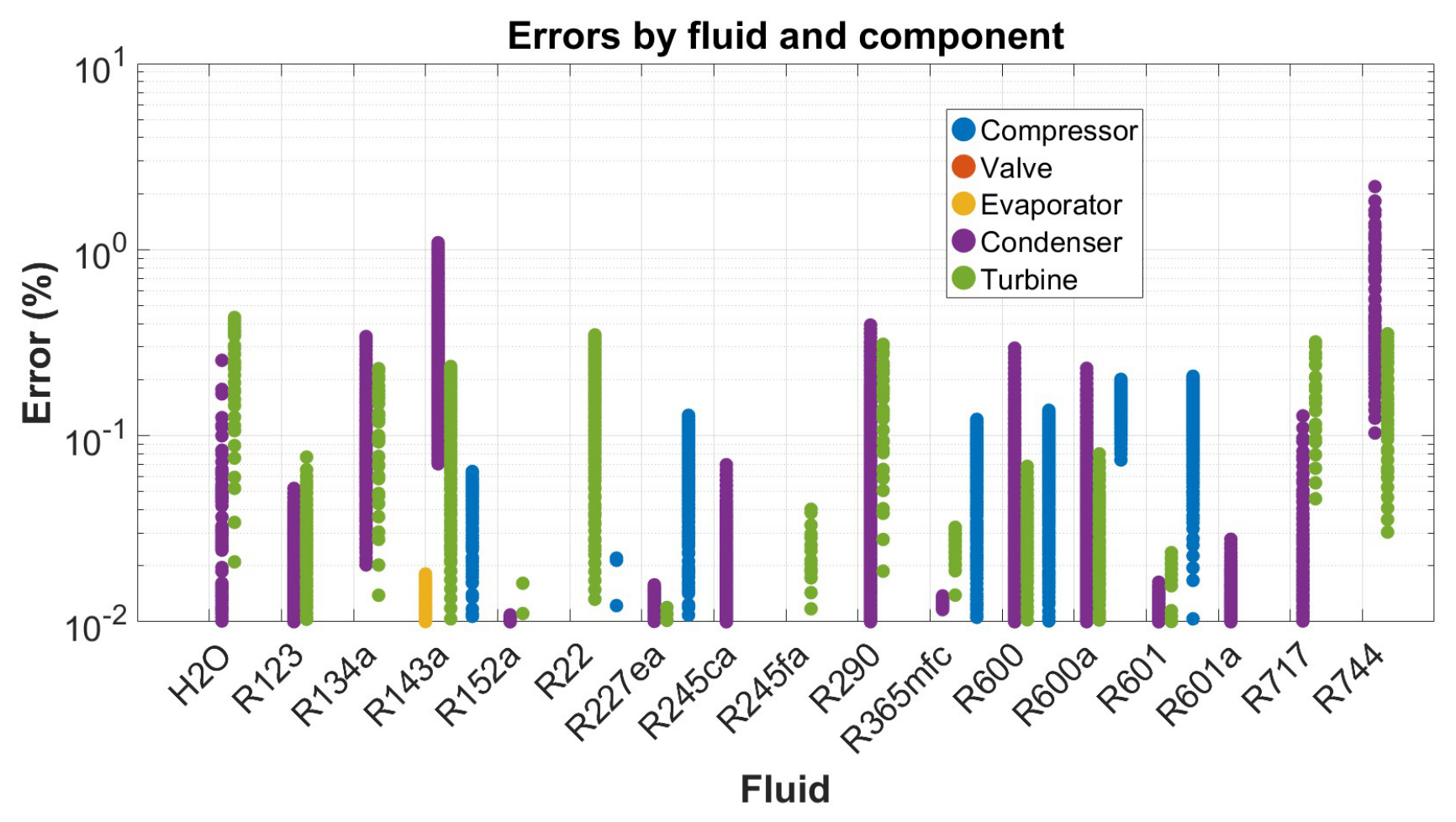
Figure 12 shows the relative errors distributed by fluid. For all tested fluids, the errors remain below for the vast majority of components, with only the condenser exhibiting isolated points reaching up to (for CO2 in transcritical operation). This isolated peak is due to the inherent limitations of the fluid model near the critical point of CO2. No systematic bias is observed in the error distribution; the deviations are symmetrically and homogeneously scattered around zero. The overall agreement is remarkably robust, with all errors remaining below even in the most unfavorable case. For most components and fluids, the error is well below .
These results validate the use of the thermodynamic overall temperature as an accurate, elegant, and unifying parameter for the exergy analysis of real flows with dissipation. The explicit simplified formulas are sufficiently accurate for engineering applications, particularly pinch analysis, system design, and multi-energy network simulation. The physical interpretation of the results confirms that the approach is fundamentally sound and numerically stable, with the highest errors localized in regions of strong thermodynamic non-linearities (CO2 transcritical, water wet region, heavy hydrocarbons in compression), which do not compromise the overall validity of the method.
5. Conclusions
This paper has introduced the concept of thermodynamic overall temperature as a simple and unique parameter to characterize the quality of streams in real energy components. The main contributions are:
- 1.
- The development of a general expression for the exergy of any real thermodynamic stream by using the Carnot form equation:where is explicitly given as a function both of the temperature level and the internal dissipations of the stream. This formulation unifies the treatment of ideal and real flows, whether isobaric or with pressure drops, with or without phase change.
- 2.
- Explicit formulas for exergy losses and efficiencies have been established for key components: compressors, pumps, turbines, expansion valves, heat exchangers (with and without phase change), and pipe sections. These formulas are summarized in two comprehensive tables, providing a ready-to-use reference for engineers and researchers.
- 3.
- The proposed method extends classical pinch analysis to real flows by integrating pressure drops and mechanical components, without requiring complex numerical simulations. The hot or cold character of a stream is redefined by considering its exergy level, characterized not only by its enthalpy change but also by its temperature level. A stream under compression is thus a cold stream whose heating is ensured with electricity consumption; a stream under expansion is a hot stream whose cooling is ensured with electricity production in a turbine or with complete dissipation in a valve.
- 4.
- The numerical validation conducted on 16 fluids (water, R134a, R290, ammonia, CO2, etc.) shows excellent agreement with exact exergy calculations. The relative errors are very low: maximums of 0.22% for the compressor (mean 0.05%), 0.45% for the turbine (mean 0.08%), 0.02% for the evaporator (mean 0.01%), and 2.2% for the condenser (mean 0.20%). The valve presents a nearly zero error (machine precision). All errors remain below 2.2% in the worst case (transcritical CO2), and for most components they are well below 0.5%. These results confirm the robustness of the overall temperature approach for engineering applications.
- 5.
- The validation confirms that the thermodynamic overall temperature approach is applicable to a wide range of fluids, from simple ideal gases to complex refrigerants and natural fluids. The explicit formulas are sufficiently accurate for engineering applications, provided that an accurate fluid model is used in the critical region. The method is particularly attractive as it replaces iterative local calculations with a single closed-form expression, significantly reducing computational time while maintaining accuracy.
The concept of thermodynamic overall temperature bridges the gap between the idealized logarithmic mean temperature (valid at constant pressure) and real processes with dissipation. It naturally incorporates isentropic efficiencies and phase changes via zonal decomposition. This framework facilitates the optimization of multi-energy networks (electricity, heating, cooling, energy, CO2) by providing a simple, physically based exergy criterion.
Future work will focus on integrating this method into simulation environments for district heating and cooling networks, as well as extending it to reactive systems and combined heat and power plants. The proposed approach also opens perspectives for exergoeconomic optimization, where the cost of exergy destruction can be directly related to the thermodynamic overall temperature of each stream.
Supplementary Materials
The ADVENS Props library used for validation is available from the corresponding author upon reasonable request.
Author Contributions
Conceptualization, M.K. and S.E.; methodology, M.K. and S.E.; software, M.K. and S.E.; validation, M.K. and S.E.; formal analysis, M.K. and S.E.; investigation, M.K. and S.E.; resources, M.K.; data curation, S.E.; writing—original draft preparation, M.K. and S.E.; writing—review and editing, M.K. and S.E.; visualization, S.E.; supervision, M.K.; project administration, M.K.; funding acquisition, M.K.; funding acquisition, M.K. All authors have read and agreed to the published version of the manuscript.
Funding
This research received no external funding.
Data Availability Statement
Data is contained within the article.
Acknowledgments
The authors acknowledge the EPFL (Ecole Polytechnique Fédérale de Lausanne), the HEIA-FR (Haute École d’Ingénierie et d’Architecture de Fribourg, HES-SO), the HEIG-VD (HES-SO Vaud), and the UCAD (Faculté des Sciences et Techniques, Dakar) for their institutional and logistical support throughout this research.
Conflicts of Interest
The authors declare no conflicts of interest.
Nomenclature
| ambient temperature | |
| energy efficiency () | |
| isentropic efficiencies of compressor, pump, turbine, valve, and piping | |
| dissipation factors due to pressure drops in superheating and subcooling | |
| overall thermodynamic mean temperatures of hot, cold, and useful streams | |
| logarithmic mean temperature at outlet pressure | |
| boiling point temperature | |
| critical temperature | |
| superheating degree | |
| subcooling degree | |
| saturation temperature | |
| enthalpy variations (subcooled, two-phase, superheated zones) | |
| transformation energy flow | |
| exergy received (work) | |
| exergy received from hot fluid | |
| exergy provided to cold fluid | |
| losses by dissipation and heat transfer |
| Roman symbols | |||
| Symbol | Unit | Definition | |
| A | m2 | Heat exchange surface area | |
| J/(kg·K) | Specific heat capacity at constant pressure | ||
| h | J/kg | Specific enthalpy | |
| k | J/kg | Specific co-enthalpy, | |
| W | Exergy destruction rate (internal losses) | ||
| kg/s | Mass flow rate | ||
| P | Pa | Absolute pressure | |
| s | J/(kg·K) | Specific entropy | |
| T | K | Absolute fluid temperature | |
| K | Ambient (environment) temperature | ||
| K | Temperature after ideal isentropic transformation | ||
| K | Saturation temperature | ||
| K | Boiling point temperature | ||
| K | Critical temperature | ||
| K | Superheating degree | ||
| K | Subcooling degree | ||
| K | Thermodynamic overall temperature, | ||
| K | Logarithmic mean temperature at constant pressure | ||
| K | Logarithmic mean temperature at discharge pressure | ||
| m3/kg | Specific volume | ||
| W | Mechanical power (work) | ||
| Greek symbols | |||
| Symbol | Unit | Definition | |
| – | Ratio of heat capacities, | ||
| – | Isentropic coefficient, | ||
| – | Energy efficiency of component () | ||
| – | Exergy efficiency (global) of component | ||
| – | Generic dissipation factor (for any stream) | ||
| – | Isentropic efficiency of compressor | ||
| – | Isentropic efficiency of turbine | ||
| – | Isentropic efficiency of pump | ||
| – | Isentropic efficiency of expansion valve | ||
| – | Polytropic efficiency (perfect gas) | ||
| – | Dissipation factor by pressure drops (hot stream) | ||
| – | Dissipation factor by pressure drops (cold stream) | ||
| – | Dissipation factor in piping | ||
| – | Carnot factor, | ||
| – | Pressure ratio, | ||
| – | Temperature ratio, | ||
| – | Polytropic caloric factor, | ||
| Indices, exponents and abbreviations | |||
| Index / Exponent | Meaning | Abbreviation | Meaning |
| a | Relative to the environment (ambient) | COP | Coefficient of performance |
| c | Relative to the cold stream | ORC | Organic Rankine cycle |
| h | Relative to the hot stream | DHN | District heating network |
| s | Isentropic or saturation state (depending on context) | HP | Heat pump |
| Subcooled zone (subcooling) | LMTD | Logarithmic mean temperature difference | |
| Superheated zone (superheating) | PCHE | Printed circuit heat exchanger | |
| Liquid-vapor phase change | EGM | Entropy generation minimization | |
| Component inlet | ADVENS | Advanced energy system simulation software | |
| Component outlet | CoolProp | Open-source thermophysical property library | |
| + | Exergy received by the system (input) | – | – |
| − | Exergy provided by the system (output) | – | – |
References
- Blanke, C.; Kane, M. An object-oriented implementation of a recursive “quantum network” solver and its application to district heating networks. Energy 2025, 321, 127260. [Google Scholar]
- Gouy, L. G. Sur l’énergie utilisable. J. De Phys. Théorique Et. Appliquée 1889, 8(1), 501–518. [Google Scholar] [CrossRef]
- Darrieus, M. G. L’évolution des centrales thermiques et la notion d’énergie utilisable. Sci. Et. Ind. 1931, 15(206), 122–126. [Google Scholar]
- Keenan, J. H. A steam chart for second-law analysis: A study of thermodynamic availability in the steam power plant. Mech. Eng. 1932, 54(3), 195–204. [Google Scholar]
- Keenan, J. H. Availability and irreversibility in thermodynamics. Br. J. Appl. Phys. 1951, 2(7), 183–192. [Google Scholar] [CrossRef]
- Rant, Z. Exergie, ein neues Wort für “Technische Arbeitsfähigkeit”. Forsch. Im. Ingenieurwesen 1956, 22(1), 36–37. [Google Scholar] [CrossRef] [PubMed]
- Bejan, A. Fundamentals of exergy analysis, entropy generation minimization, and the generation of flow architecture. Int. J. Energy Res. 2002, 26(7), 545–565. [Google Scholar] [CrossRef]
- Borel, L.; Favrat, D. Thermodynamics and Energy Systems Analysis: From Energy to Exergy; EPFL Press: Lausanne, Switzerland, 2010. [Google Scholar]
- Kotas, T. J. The Exergy Method of Thermal Plant Analysis; Butterworths: London, UK, 1985. [Google Scholar]
- Favrat, D.; Kane, M. Exergy Analysis of Heating and Cooling: Exergy analyses of basic components of heating or cooling systems; Elsevier, 2024. [Google Scholar]
- Meunier, F.; Poyelle, F.; LeVan, M. D. Second-law analysis of adsorptive refrigeration cycles: The role of thermal coupling entropy production. Appl. Therm. Eng. 1996, 16(12), 925–938. [Google Scholar]
- Marquet, P. On the concept of exergy and available enthalpy: Application to atmospheric energetics. Q. J. R. Meteorol. Soc. 1991, 117(502), 1099–1149. [Google Scholar] [CrossRef]
- Maxwell, J. C. Theory of Heat; Longmans, Green, and Co.: London, UK, 1871. [Google Scholar]
- Gibbs, J. W. Graphical methods in the thermodynamics of fluids. Trans. Connect. Acad. Arts Sci. 1873, 2, 309–342. [Google Scholar]
- Staine, F. Intégration énergétique de procédés industriels par la méthode du pincement étendue aux facteurs exergétiques. Thèse de doctorat, École Polytechnique Fédérale de Lausanne, Lausanne, Suisse, 1995. [Google Scholar] [CrossRef]
- Ziegler, F. Relationships between temperature differences in heat exchangers of heat transformation devices. Rev. Générale De Therm. 1998, 37(7), 549–555. [Google Scholar]
- Schiffmann, J.; Favrat, D. Application of exergy balances for the optimization of non-adiabatic small turbomachines operation. Energy 2011, 36(5), 2924–2936. [Google Scholar] [CrossRef]
- Khennich, M.; Sorin, M.; Galanis, N. Equivalent temperature-enthalpy diagram for the study of ejector refrigeration systems. Entropy 2014, 16, 2669–2685. [Google Scholar] [CrossRef]
- Meunier, F.; Neveu, P.; Castaing-Lasvignottes, J. Equivalent Carnot cycles for sorption refrigeration. Int. J. Refrig. 1998, 21(6), 472–489. [Google Scholar]
- Castaing-Lasvignottes, J.; Neveu, P. Equivalent Carnot cycle concept applied to thermochemical solid/gas resorption systems. Int. J. Refrig. 1998, 21(1), 58–69. [Google Scholar]
- Neveu, P. Apports de la thermodynamique pour la conception et l’intégration des procédés. Habilitation à Diriger des Recherches, Université de Perpignan, Perpignan, France, 2002. [Google Scholar]
- Clausius, R. On several convenient forms of the fundamental equations of the mechanical theory of heat. In The Mechanical Theory of Heat: With Its Applications to the Steam-engine and to the Physical Properties of Bodies; J. Van Voorst: London, UK, 1867; pp. 327–365. [Google Scholar]
- Prigogine, I. Introduction to Thermodynamics of Irreversible Processes; Interscience Publishers: New York, NY, USA, 1962. [Google Scholar]
- Bejan, A. Entropy Generation through Heat and Fluid Flow; John Wiley & Sons: New York, NY, USA, 1982. [Google Scholar]
- Van Wylen, G. J.; Sonntag, R. E. Fundamentals of Classical Thermodynamics; John Wiley & Sons: New York, NY, USA, 1973. [Google Scholar]
- Canivet, Y. Analyse Entropique et Exergétique des Systèmes Énergétiques par des Représentations Géométriques. Thèse de doctorat, Université Paris Nanterre, Nanterre, France, 2017. [Google Scholar] [CrossRef]
- Leff, H. S. Thermodynamic entropy: The spreading and sharing of energy. Am. J. Phys. 1996, 64(10), 1261–1271. [Google Scholar] [CrossRef]
- Poredoš, P.; Kitanovski, A.; Poredoš, A. Exergy analysis of low-temperature district heating systems with different sanitary hot-water boosters. Entropy 2019, 21(4), 388. [Google Scholar] [CrossRef] [PubMed]
- Adihou, Y. Modélisation et optimisation exergétique des réseaux thermiques basse température. Thèse de doctorat, Université Savoie Mont Blanc, Chambéry, France, 2022. [Google Scholar]
- Sharew, S. S.; Di Pretoro, A.; Yimam, A.; Negny, S.; Montastruc, L. Combining exergy and pinch analysis for the operating mode optimization of a steam turbine cogeneration plant in Wonji-Shoa, Ethiopia. Entropy 2024, 26(6), 453. [Google Scholar] [CrossRef] [PubMed]
- Criado-Sancho, M.; Jou, D.; Casas-Vázquez, J. Caloric and entropic temperatures in non-equilibrium steady states. Phys. Rev. E 2016, 93(4), 042104. [Google Scholar] [CrossRef] [PubMed]
- Yang, X.; Xu, J.; Miao, Z.; Zou, J.; Qi, F. The definition of non-dimensional integration temperature difference and its effect on organic Rankine cycle. Appl. Energy 2016, 167, 17–33. [Google Scholar] [CrossRef]
- Dong, Z.; Du, Q. The local distribution of temperatures and entropy generation rate in an ideal counterflow heat exchanger. Coatings 2021, 11(8), 970. [Google Scholar] [CrossRef]
- Allahverdyan, A. E.; Gevorkian, S. G.; Dyakov, Y. A.; Wang, P.-K. Thermodynamic definition of mean temperature. Phys. Rev. E 2023, 108(4), 044112. [Google Scholar] [CrossRef] [PubMed]
- Landau, L. D.; Lifshitz, E. M. Statistical Physics, Part 1; Pergamon Press: Oxford, UK, 1980. [Google Scholar]
- Casas-Vázquez, J.; Jou, D. Temperature in non-equilibrium states: A review of open problems and current proposals. Rep. Prog. Phys. 2003, 66(11), 1937–2023. [Google Scholar] [CrossRef]
- Bell, I. H.; Wronski, J.; Quoilin, S.; Lemort, V. Pure and pseudo-pure fluid thermophysical property evaluation and the open-source thermophysical property library CoolProp. Ind. Eng. Chem. Res. 2014, 53(6), 2498–2508. [Google Scholar] [CrossRef] [PubMed]
Figure 1.
T-s diagram for calculating the entropy variation at constant pressure.
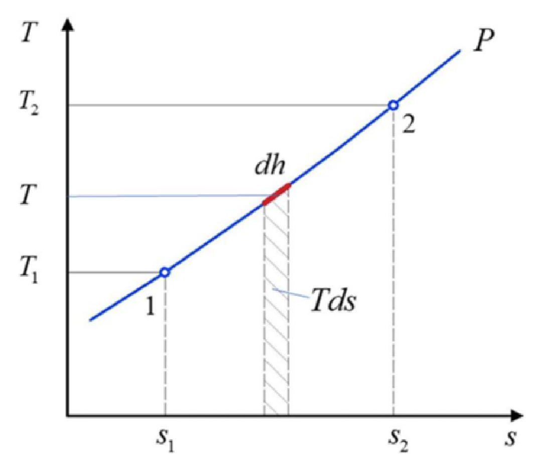
Figure 2.
Comparison between the average temperature and the logarithmic mean temperature.
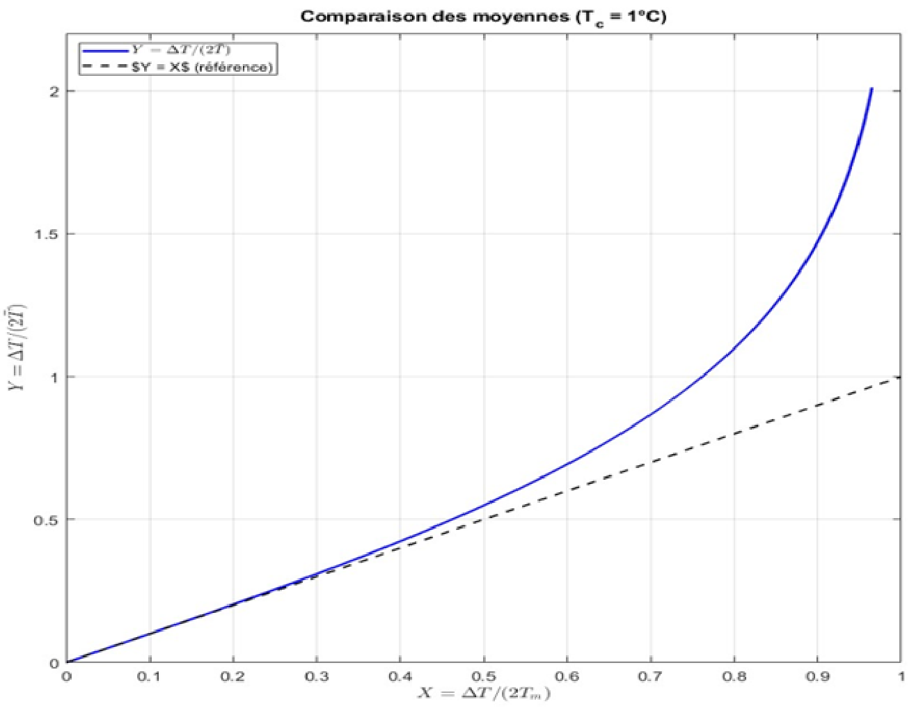
Figure 3.
T-s diagram of a hot stream in condensation, showing the three zones: superheating (g), two-phase (b), and subcooling (l).
Figure 3.
T-s diagram of a hot stream in condensation, showing the three zones: superheating (g), two-phase (b), and subcooling (l).
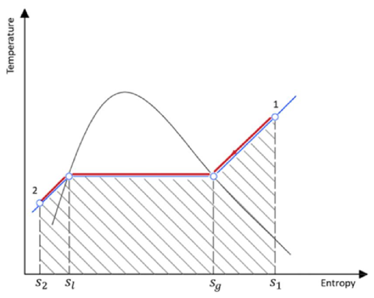
Figure 4.
T-s diagram of hot and cold streams providing heat to a system, with pressure drop and dissipation losses: (a) The hot stream, where the real path () is decomposed into an isentropic expansion () followed by an isobaric cooling (); and (b) The cold stream, where the real path () is decomposed into an isentropic expansion () followed by an isobaric heating ().
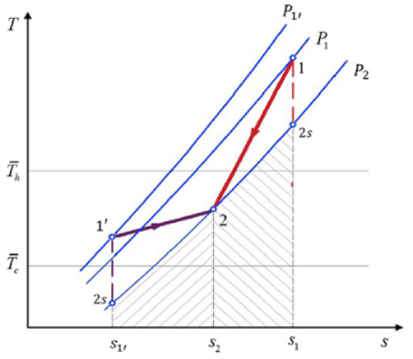
Figure 5.
(left) Scheme of a compression process in an adiabatic compressor. (right) T-s diagram of a compression process showing the real path () and the isentropic reference path ().
Figure 5.
(left) Scheme of a compression process in an adiabatic compressor. (right) T-s diagram of a compression process showing the real path () and the isentropic reference path ().
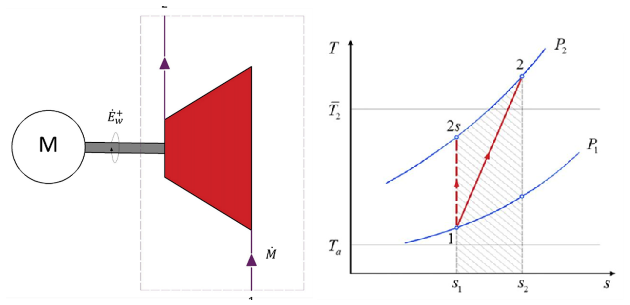
Figure 6.
Effect of the thermodynamic overall temperature on the specific exergy losses and exergy efficiency of a compressor.
Figure 6.
Effect of the thermodynamic overall temperature on the specific exergy losses and exergy efficiency of a compressor.
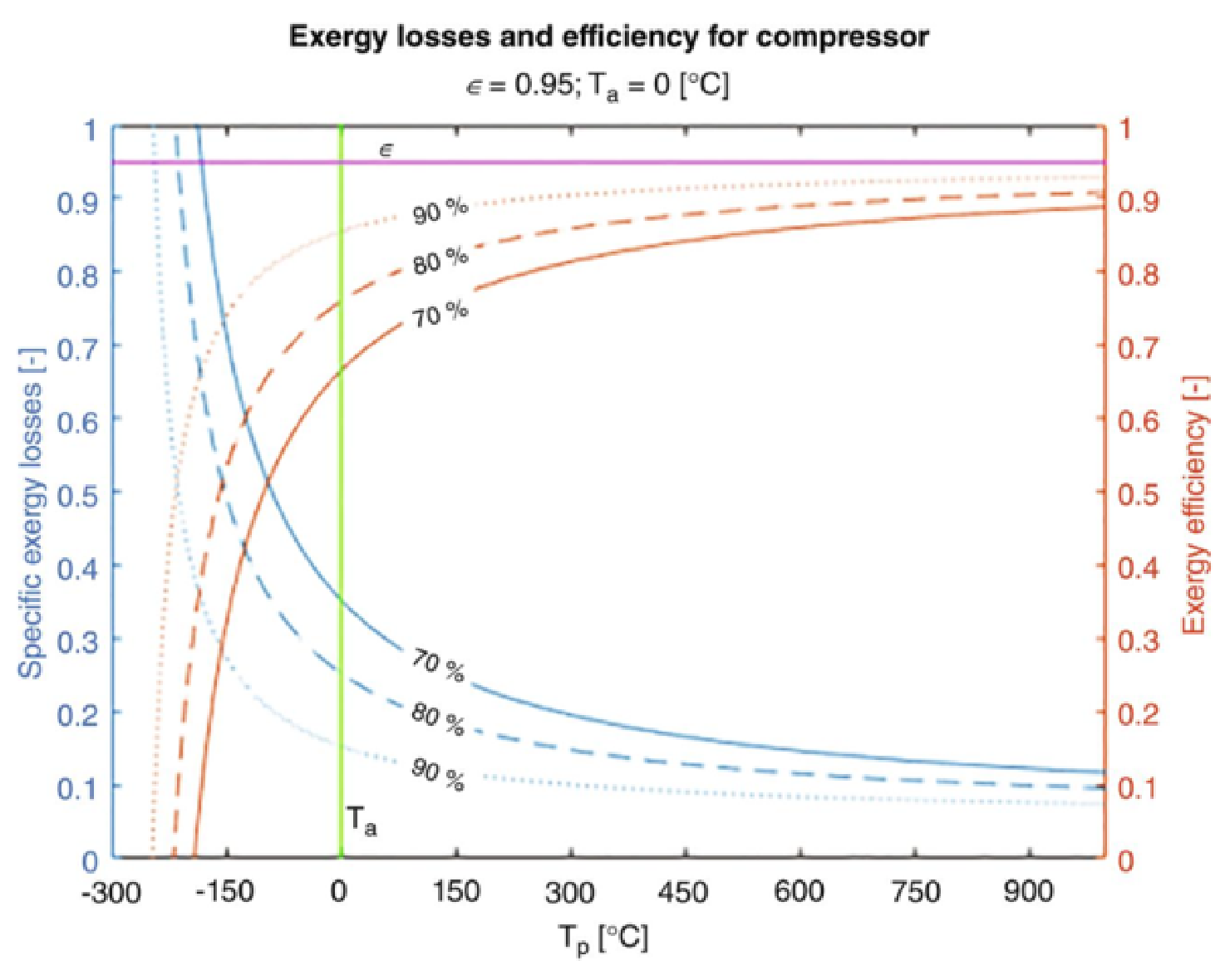
Figure 7.
(left) Scheme of an expansion process in an adiabatic turbine. (right) T-s diagram of an expansion process showing the real path () and the isentropic reference path ().
Figure 7.
(left) Scheme of an expansion process in an adiabatic turbine. (right) T-s diagram of an expansion process showing the real path () and the isentropic reference path ().
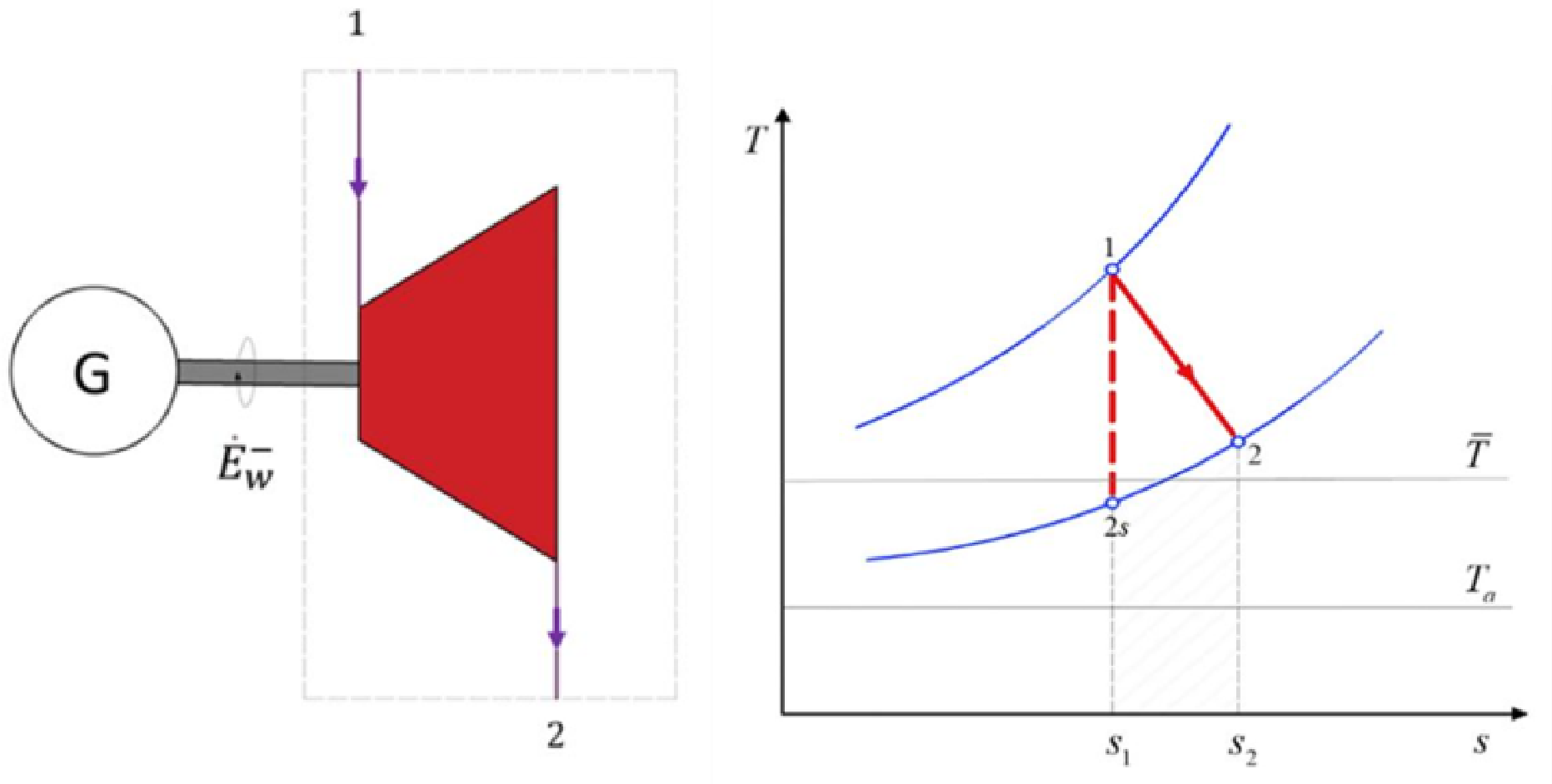
Figure 8.
Effect of the thermodynamic overall temperature on the specific exergy losses and exergy efficiency of a turbine.
Figure 8.
Effect of the thermodynamic overall temperature on the specific exergy losses and exergy efficiency of a turbine.
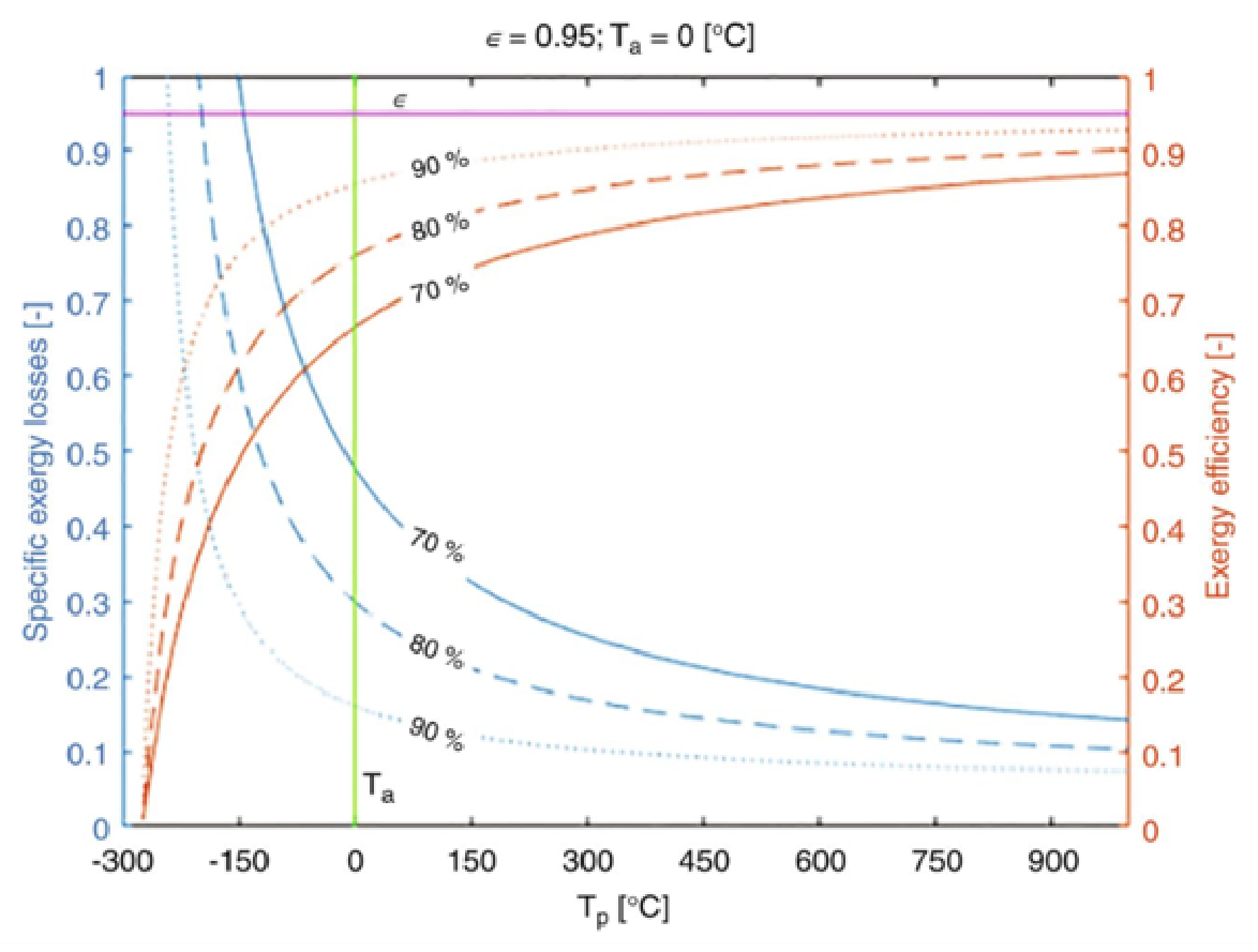
Figure 9.
Effect of the thermodynamic overall temperature on the specific exergy losses of an expansion valve.
Figure 9.
Effect of the thermodynamic overall temperature on the specific exergy losses of an expansion valve.
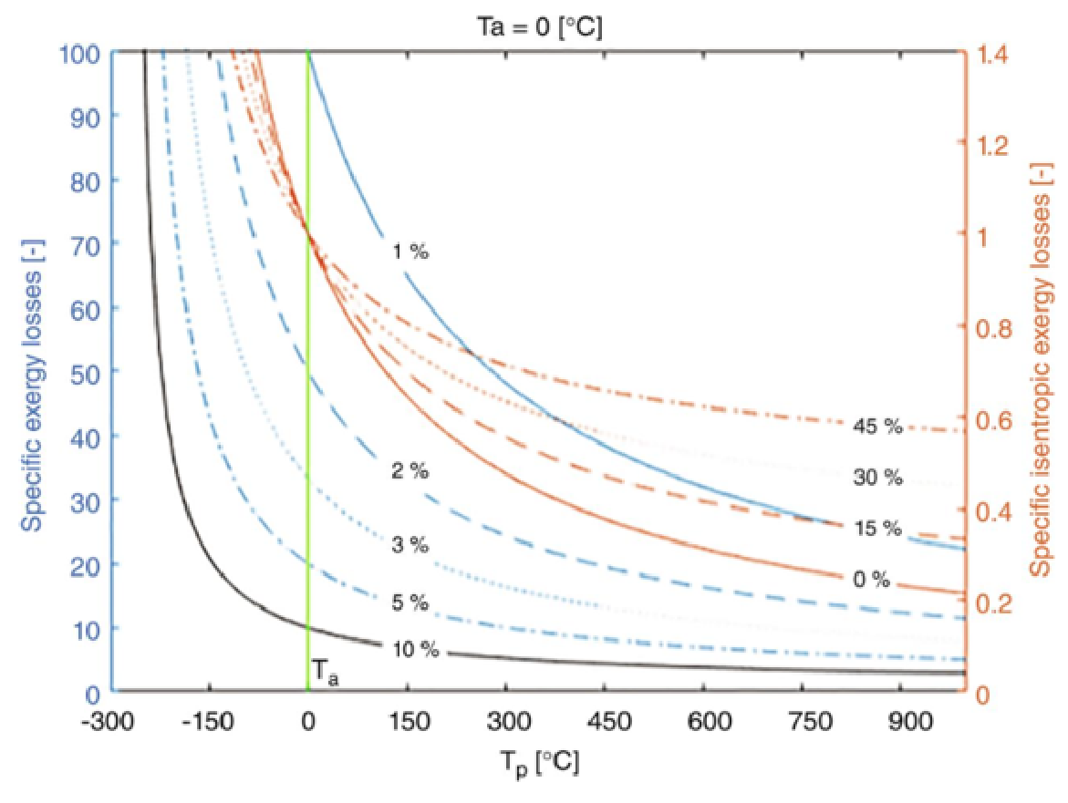
Figure 10.
Thermodynamic overall temperature as a function of the isentropic dissipation factor . The diagram maps the different transfer and dissipation regimes: piping zones (), cold heat exchanger (), hot heat exchanger or compressor (), and expansion (turbine, valve, cooled compressor, ). The violet points highlight the remarkable behavior at the cooled plateau . The negative values of for characterize the nature of expansion processes (decrease in enthalpy and increase in entropy).
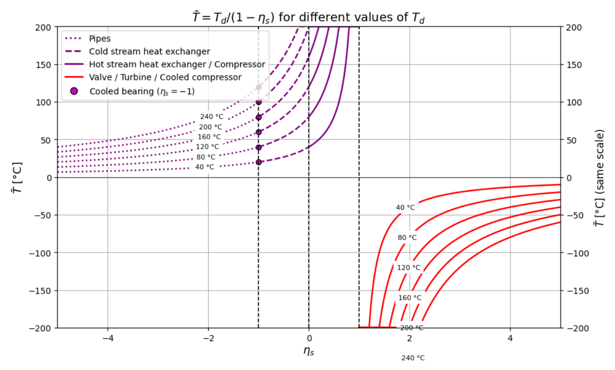
Figure 11.
Distribution of relative errors by component.
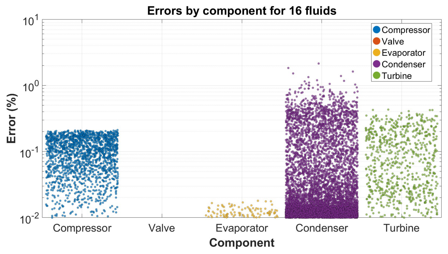
Figure 12.
Distribution of relative errors by refrigerant fluid.
Disclaimer/Publisher’s Note: The statements, opinions and data contained in all publications are solely those of the individual author(s) and contributor(s) and not of MDPI and/or the editor(s). MDPI and/or the editor(s) disclaim responsibility for any injury to people or property resulting from any ideas, methods, instructions or products referred to in the content. |
© 2026 by the authors. Licensee MDPI, Basel, Switzerland. This article is an open access article distributed under the terms and conditions of the Creative Commons Attribution (CC BY) license (http://creativecommons.org/licenses/by/4.0/).
Copyright: This open access article is published under a Creative Commons CC BY 4.0 license, which permit the free download, distribution, and reuse, provided that the author and preprint are cited in any reuse.