

Submitted:
25 September 2026
Posted:
28 September 2026
You are already at the latest version
Abstract
Groundwater contamination by 90Sr remains an important component of the long-term environmental impact of the Chornobyl accident, while the spatial coverage of monitoring observations limits direct assessment of contamination patterns across the Chornobyl Exclusion Zone (CEZ). This study evaluates the applicability of machine-learning methods for regional assessment of 90Sr groundwater contamination and identification of its principal controlling factors. Random Forest (RF) and XGBoost models were developed using groundwater 90Sr observations for 2015-2020 and source-related, hydrogeological, geochemical, topographic, and monitoring-well predictors. Performance was evaluated using repeated stratified holdout validation for multiclass classification and complementary regression of log-transformed 90Sr concentrations. Regional contamination classes were subsequently predicted using spatially distributed predictor layers. The RF classifier, predicting order-of-magnitude concentration classes, achieved a mean accuracy of 0.70 and weighted F1-score of 0.66, compared with 0.64 and 0.62 for XGBoost, whereas XGBoost showed slightly higher regression performance (R2 = 0.55) than RF (R2= 0.50). Across model-specific, permutation and SHAP analyses, groundwater-table depth, aquifer sampling depth, and surface 90Sr contamination were repeatedly identified among the most influential predictors. Spatial predictions indicated that higher contamination classes were localized and primarily associated with the combination of elevated surface contamination and shallow groundwater conditions, with notable correspondence to radioactive-waste disposal areas. The results provide spatial information to support prioritization and development of groundwater monitoring networks in the CEZ.
Keywords:
90Sr
; groundwater contamination
; machine learning
; spatial prediction
; contamination risk mapping
; Chornobyl exclusion zone
1. Introduction
Radioactive contamination of groundwater has been recognized since the early period following the 1986 Chornobyl accident as a potentially important pathway for radionuclide migration within the Chornobyl Exclusion Zone (CEZ) and for their eventual transfer to the Pripyat–Dnipro River system (Figure 1) [1,2,3]. The hydrogeological conditions of the CEZ, characterized by a shallow unconfined aquifer in permeable sandy Quaternary deposits and relatively high infiltration rates, favour interaction between contaminated surface and near-surface sources of radioactivity, groundwater, and surface-water bodies. Although previous modelling and long-term monitoring studies indicate that groundwater transport is unlikely to cause unacceptable radiological impacts outside the CEZ, groundwater remains an important component of long-term environmental surveillance and management of radioactively contaminated legacy sites and licensed radioactive waste disposal facilities in the CEZ [4,5,6,7,8].
Among the Chornobyl-derived radionuclides, ⁹⁰Sr is presently the principal contaminant of concern in groundwater because of its comparatively high mobility in soils and aquifers. In contrast, ¹³⁷Cs and transuranic radionuclides are generally much more strongly retained by geological media and occur in groundwater at considerably lower concentrations [8,10]. Monitoring data show pronounced spatial variability of ⁹⁰Sr concentrations, with elevated levels particularly associated with radioactive waste dump sites, the ChNPP industrial area, and seepage from contaminated surface-water bodies. At individual locations, 90Sr concentrations in groundwater reach 10⁵–10⁶ Bq m⁻³, while still higher concentrations have been reported from detailed site investigations [11,12,13]. Subsurface transport can be locally important for the contamination of small rivers and former agricultural drainage systems in the CEZ, particularly where contaminated groundwater discharges directly to surface-water bodies and during low-flow conditions [14,15]. Reliable identification of areas with an elevated probability of groundwater contamination is therefore relevant both for assessing potential impacts on connected surface-water systems and for prioritizing groundwater monitoring and protection measures.
The existing groundwater monitoring system in the CEZ provides a unique long-term dataset, but it was developed progressively over several decades with focus on specific facilities (such as “Shelter” object containing damaged Unit 4, radioactive waste disposal sites, Chornobyl NPP cooling pond, etc.) and therefore does not provide spatially uniform coverage of the radioactively contaminated territory [4,8]. These limitations provide a strong rationale for developing spatial prediction methods capable of identifying areas in the CEZ where elevated groundwater contamination is more likely to occur.
Mechanistic modelling of ⁹⁰Sr migration at the regional scale is challenging because contaminant transport is governed by numerous spatially variable hydrogeological, geochemical, biological, and anthropogenic factors, which are discussed in more detail in the following section. The complexity and spatial variability of these processes, together with the limited availability of data needed to characterize them, limit the feasibility and reliability of fully mechanistic regional-scale modelling of contaminant transport in soils and groundwater. These limitations provide a rationale for complementing process-based models with machine-learning approaches [16,17].
Machine learning methods are increasingly applied in analyzing and predicting contaminant distributions in soils and groundwater due to their efficiency, and potential to capture complex nonlinear relationships [17,18,19,20]. Groundwater-quality studies employing machine learning (ML) have predominantly focused on nitrate as the target contaminant, followed by the Water Quality Index (WQI) and arsenic [18]. More recently, a growing number of studies have applied ML approaches to the assessment and prediction of heavy-metal contamination in groundwater [21,22,23]. Fallatah et al. (2022) [24] applied ML algorithms to analyse naturally occurring α- and β-radioactivity in groundwater in Saudi Arabia. However, to the best of our knowledge, the prediction of artificial radionuclide concentrations in groundwater using ML methods has not yet been addressed in the scientific literature.
Although the general ML methodology applicable to artificial radionuclides can be expected to be similar to that used for other inorganic anthropogenic contaminants, important differences arise from contaminant-specific source-term characteristics and geochemical behaviour. These features should therefore be reflected in the selection and engineering of predictor variables for ML models targeting artificial radionuclide contamination of groundwater. Accordingly, the selection of predictor variables in this study was guided by a physics-informed approach based on a conceptual framework encompassing several groups of controlling factors: pollution sources, environmental media, contaminant transport processes and technical characteristics of monitoring wells.
Because depth to the groundwater table is expected to influence the potential for radionuclide migration from near-surface contamination sources to the unconfined aquifer, its regional distribution was estimated using a three-dimensional groundwater-flow model of the CEZ calibrated against groundwater-level monitoring data.
Based on a recent literature review, Random Forest (RF) and Extreme Gradient Boosting (XGBoost) are among the most frequently used machine-learning models in groundwater contamination studies [19]. These tree-based ensemble models have demonstrated good performance in handling relatively small datasets, high-dimensional predictor spaces, and complex nonlinear relationships. They are also methodologically well established and have been widely applied in practical environmental modelling and assessment studies [18,19].
Integration of ML with GIS provides an effective framework for regional contamination assessment by combining the ability of ML to identify complex relationships between contamination and its controlling factors with GIS capabilities for integrating spatial datasets and extrapolating model predictions to produce regional contamination and risk maps [19,25].
In the present study, machine-learning methods combined with GIS analysis are used to predict areas of the CEZ characterized by an elevated risk of 90Sr groundwater contamination and to identify the principal environmental and source-related factors controlling the observed contamination levels.
Data from 86 groundwater monitoring wells tapping the local unconfined aquifer in the sandy Quaternary deposits operated by State Special Enterprise “Ecocenter”, which is responsible for radiation monitoring in the CEZ, were used in this study.
To enhance the practical applicability of the prediction model, an interval-based classification approach was employed, in which groundwater 90Sr concentrations were treated as a categorical target variable, with each concentration class spanning one order of magnitude (Bq/m3). Classification of contaminant concentrations into discrete ranges has been used in previous ML-based environmental assessments, including direct classification by order-of-magnitude concentration intervals [26].
The resulting spatial predictions are intended to complement the existing observation network, provide a quantitative basis for prioritizing further development and modernization of groundwater monitoring in the CEZ, and support risk assessment and the planning of water-protection and remediation measures.
Conceptual workflow of the study is shown in Figure 2.
2. Groundwater Contamination by 90Sr in the Chornobyl Exclusion Zone
2.1. Site Hydrogeology and Groundwater Contamination Sources
From the viewpoint of groundwater contamination, the most relevant hydrogeological unit is the uppermost unconfined aquifer hosted by permeable Quaternary sandy deposits. The aquifer is composed mainly of Pliocene and Pleistocene–Holocene alluvial, fluvioglacial and aeolian sands and is underlain by the low-permeability clay–marl deposits of the Eocene Kyiv Suite, which form a regional aquitard separating it from deeper confined aquifers. Groundwater conditions vary systematically with geomorphology. The depth to the water table is typically 0–2 m in the Pripyat River floodplain, about 2–7 m on river terraces, and may reach 14–17 m in the fluvioglacial plateau in the Pripyat–Uzh interfluve. The saturated thickness of the unconfined aquifer is generally about 20–30 m and its transmissivity is of the order of 40–400 m2 d-1. Regional groundwater flow is directed toward the Pripyat River and its tributaries, with hydraulic gradients generally around 0.001–0.003 [2,4,27]. Recharge is spatially variable and depends on geomorphology, vegetation and land disturbance; values of about 200 ± 50 mm y-1 have been estimated for the disturbed Red Forest area [12].
At the regional scale, the principal distributed source term of ⁹⁰Sr is topsoil contaminated by radioactive fallout from the destroyed Unit 4 of the Chornobyl NPP [28]. Most of the ⁹⁰Sr released during the 1986 accident was initially associated with micron-sized nuclear fuel particles and was progressively mobilized as these particles weathered and their uranium-oxide matrix dissolved [29,30]. A major redistribution of contamination occurred during accident-mitigation and cleanup works around the ChNPP in 1986–1988. Contaminated soil and vegetation, including pine trees from the “Red Forest”, together with debris from demolished buildings and other radioactive materials, were buried in situ in shallow trenches, generally 2–3 m deep, or bulldozed into above-ground mounds. The decontaminated area around the ChNPP covered approximately 10 km2; the total number of waste burials has been estimated at 800–1000, containing about 1.2 million m3 of buried radioactive material [31]. Because the groundwater table is locally shallow and seasonally variable, some trenches may be intermittently inundated and act as important secondary sources of 90Sr to groundwater [11,12]. Additional local sources are contaminated surface-water bodies and their bottom sediments contaminated with fuel-particles. Depending on local hydraulic head gradients towards the Pripyat River, seepage through sediments can generate 90Sr-contaminated groundwater moving toward the river [4,8].
2.2. Groundwater Monitoring Program of Ecocenter
The main regional groundwater monitoring programme in the CEZ is operated by the State Specialized Enterprise (SSE) “Ecocenter” and currently includes approximately 150 monitoring wells mostly situated in the 10-km zone of ChNPP, with primary emphasis on the unconfined aquifer in Quaternary deposits [4,8]. The network covers the principal potential sources and receptor areas, including radioactive-waste dump sites, engineered radioactive waste disposal sites and the former ChNPP cooling pond and adjacent contaminated lakes. The principal monitored parameters are groundwater level and ⁹⁰Sr and ¹³⁷Cs activity concentrations; sampling frequency varies from monthly to once every six months depending on the site. The core near-zone network was installed in 1989–1991 and includes many wells with iron casing and long (~12 m) screens, whereas later extensions introduced PVC-cased wells and multilevel clusters with shorter screens. These design differences are important for interpretation of the monitoring data because long-screen wells can produce vertically averaged samples and may underrepresent strong vertical concentration gradients [8]. The field sampling and analytical methods used by SSE “Ecocenter” are described in detail by Bugai et al. (2022) [4].
Spatial distribution of mean ⁹⁰Sr groundwater concentrations for the period 2015-2020 in monitoring wells of the SSE “Ecocenter” which is used as a target variable in the subsequent ML analyses is shown in Figure 3. The highest 90Sr concentrations, locally reaching 105–106 Bq m-3, occur at radioactive-waste dump sites and in the vicinity of the former ChNPP cooling pond. Long-term monitoring indicates that, over recent decades, ⁹⁰Sr concentrations in groundwater have generally remained relatively stable or have slowly declined, suggesting that the contamination system has approached a quasi-steady state in which continued ⁹⁰Sr release from gradually dissolving residual nuclear fuel particles is approximately balanced, or slightly exceeded, by attenuation, dispersion, biological cycling, and radioactive decay [4].
2.3. Factors Controlling 90Sr Migration to Groundwater
In soils and aquifer sediments, dissolved radiostrontium occurs predominantly as the divalent Sr²⁺ ion, and its retention is governed mainly by reversible ion-exchange sorption on regular exchange sites associated with clay minerals and organic matter [32,33]. Consequently, the sorption distribution coefficient (Kd) of 90Sr depends strongly on the cation-exchange capacity and mineralogical composition of the geological medium. Sorption is also sensitive to groundwater chemistry because major divalent cations, particularly Ca2+, compete with radiostrontium for exchange sites [34].
Strontium is also a biochemical analogue of calcium and is readily taken up by plants through pathways involved in Ca acquisition. Such biological cycling through litterfall, decomposition and root turnover can contribute to retention and redistribution of ⁹⁰Sr within the rooting zone and within waste-burial sites overgrown by vegetation, thereby modifying the amount and timing of radionuclide available for downward migration to groundwater [35,36].
Post-Chornobyl radioecological studies suggest that 90Sr migration in soils and groundwater at the regional scale can potentially be influenced by a wide spectrum of spatially variable factors and contaminant-redistribution processes, including:
- spatial variability in groundwater recharge rates associated with geomorphology, soil and vegetation cover, and land disturbance [2];
Another potentially important factor is soil pH, because much of the 90Sr inventory deposited following the Chornobyl accident was initially incorporated into nuclear fuel particles. Fuel-particle dissolution rates leading to 90Sr release to mobile forms are strongly influenced by environmental conditions, particularly soil-solution pH, with faster dissolution generally occurring under more acidic conditions [29,30].
Consideration of the above processes guided the selection of covariates used for predicting 90Sr concentrations in groundwater with the ML models described in the following section.
3. Materials and Methods
The performance of ML models is strongly influenced by the quality and representativeness of the training data and by the selection of relevant predictor variables [17,18,19]. In this study, selection of predictor variables was guided by the conceptual understanding of the factors controlling 90Sr migration to groundwater outlined in Section 2.3, while also accounting for the availability and spatial coverage of relevant data.
The datasets used in the analysis included: (i) groundwater monitoring data from SSE “Ecocenter”, including groundwater levels, 90Sr concentrations and technical characteristics of monitoring wells; (ii) remote-sensing products and other publicly available spatial datasets; and (iii) model-derived data used to estimate groundwater-table depth in areas not directly covered by the monitoring network.
The procedures used for input-data selection, preprocessing and feature engineering are described below.
3.1. Dataset on 90Sr in Groundwater of Chornobyl Zone
The target dataset was derived from groundwater monitoring observations of the SSE “Ecocenter”. For each monitoring well, the target variable was defined as the mean ⁹⁰Sr activity concentration measured during the period 2015-2020. The use of a multi-year mean was intended to reduce the influence of short-term and year-to-year variability in monitoring data, which may arise from meteorological and hydrogeological fluctuations as well as from sampling and analytical uncertainties, and thereby to provide a more representative measure of the characteristic contamination level at each monitoring location.
The final dataset included 86 monitoring wells located mostly on the right bank of the Pripyat River. The spatial distribution of monitoring points was also considered during dataset preparation. Some individual facilities, in particular the “Buryakivka”, “Pidlisnyi” and “3rd Stage of ChNPP” engineered radioactive waste disposal sites (RWDS), have dense object-level monitoring networks consisting of several tens of wells concentrated within relatively small areas. To avoid excessive weighting of such local monitoring networks in the regional ML analysis, only one or two representative wells were retained from each of these facilities. This provided a more spatially balanced representation of groundwater contamination conditions across the study area.
Prior to calculation of the mean 90Sr concentration for each monitoring well, the individual time series for 2015-2020 were screened for anomalous values. Outliers were identified using the z-score criterion, and observations with an absolute z-score greater than 2 were excluded. The mean concentration was then calculated from the remaining observations for each well. This filtering step was intended to reduce the influence of isolated measurements that could reflect sampling, analytical, or data-entry errors.
Groundwater 90Sr concentrations span several orders of magnitude and exhibit a strongly right-skewed distribution, which is typical of contaminant-concentration datasets. The resulting mean concentrations were therefore transformed using the decimal logarithm, log10(90Sr), to compress the concentration range, reduce skewness, and improve numerical stability during model training. Log transformation is commonly applied in groundwater-quality and environmental ML studies when target variables exhibit highly skewed distributions [17,18,19].
Two alternative formulations of the target variable were evaluated. In the first case, the log₁₀-transformed ⁹⁰Sr concentration was treated as a continuous response variable and predicted using regression models. In the second case, the original ⁹⁰Sr concentrations were converted to categorical classes defined by fixed order-of-magnitude intervals, for example 102–103, 103–104 and 104–105 Bq m-3 (Figure 4). Each monitoring well was assigned to the class corresponding to its mean ⁹⁰Sr concentration.
The categorical formulation was introduced to improve the practical applicability and robustness of regional-scale predictions. Exact prediction of ⁹⁰Sr concentrations is difficult because both the monitoring data and the spatial predictor variables are characterized by substantial heterogeneity and uncertainty, whereas discrimination between successive order-of-magnitude concentration ranges represents a more realistic level of prediction accuracy for regional screening purposes. These classes also correspond to materially different contamination levels and therefore provide a convenient basis for groundwater contamination risk mapping and prioritization of monitoring locations.
3.2. Potentially Influencing Factors (Covariates)
The selected predictor variables are listed in Table 1. Their selection was intended to represent the principal components of the conceptual contaminant-migration system, including source-term characteristics, groundwater transport conditions, surface topography and vegetation cover, geochemical factors affecting ⁹⁰Sr mobility, and technical characteristics of monitoring wells that may influence the measured groundwater concentrations. The selection also took into account hydrogeological factors incorporated in the DRASTIC methodology for assessing intrinsic groundwater vulnerability to contamination [40].
The initial analysis considered a larger set of candidate predictors than those retained in Table 1. In particular, the original feature set included distance from the sampling location to the contaminant emission source (damaged Unit 4 of the ChNPP), ground-surface elevation, and site geomorphology. These variables were subsequently excluded because they showed strong correlations with predictors already retained in the model. Distance to the contaminant emission source was strongly associated with surface ⁹⁰Sr contamination density, whereas surface elevation and geomorphology were closely related to depth to the groundwater table. The highly correlated predictors were therefore removed to simplify the predictor set, reduce redundancy, and facilitate interpretation of feature-importance results.
Details on the derivation and preprocessing of the individual features used in the ML analyses and predictive modelling are provided below.
3.2.1. Source-Term Characteristics
Regional surface contamination density by 90Sr (Surface_Cont; Table 1) was derived from the soil-sampling dataset of Kashparov et al. (2018). A spatially continuous 90Sr contamination field was generated using Ordinary Kriging of log10-transformed measurements with a spherical variogram model, fitted to the experimental variogram (sill = 0.636, range = 0.154°, nugget = 0.065) (Figure 1).
For areas occupied by radioactive-waste dumps, the source term was represented by a sector-average equivalent surface contamination density. For each waste-dump sector, this quantity was calculated by dividing the estimated 90Sr activity inventory in the waste burials by the corresponding sector area (Figure 5). Activity-inventory data were obtained from the Chornobyl radioactive-waste inventory databases developed within the projects described by Antropov et al. (2001) [31] and Molitor et al. (2017) [39]. The 90Sr contamination values were decay-corrected to the reference year 2015. Consistent with the treatment of the groundwater-concentration target variable, the resulting Surface_Cont values were subsequently log10-transformed prior to ML analysis.
Groundwater monitoring locations situated within radioactive-waste dump sectors were additionally identified using the binary predictor Waste_Dump (0 = outside a waste-dump sector; 1 = within a waste-dump sector). This predictor was introduced to account for the specific source configuration and hydrogeological conditions of these sites, where radioactive material is buried in shallow trenches or mounds and may occur substantially closer to the groundwater table than fallout-derived contamination in undisturbed topsoil (Table 1).
3.2.2. Hydrogeological Conditions
Depth to the groundwater table (Depth_GWT; Table 1) at monitoring-well locations was defined as the multi-year mean groundwater-table depth for the period 2015–2020, based on monitoring data from SSE “Ecocenter”. For spatial prediction at locations not covered by the groundwater monitoring network, this parameter was estimated using the groundwater-flow model described in Section 3.3.
Depth from the groundwater table to the top of the well screen (Depth_Aquifer; Table 1) was calculated for each monitoring well using the corresponding Depth_GWT value and well-passport data on the elevation of the top of the screened interval.
3.2.3. Topographic Wetness Index (TWI)
The Topographic Wetness Index (TWI) was calculated to characterize the potential spatial distribution of soil moisture and the tendency for water accumulation controlled by topography. The index combines information on the upstream contributing area and local slope, allowing identification of locations where runoff is expected to concentrate [41,42].
A Shuttle Radar Topography Mission (SRTM) Digital Elevation Model (DEM) with a spatial resolution of approximately 30 m was used as the elevation source. Prior to hydrological analysis, artificial depressions in the DEM were removed using the Breach Depressions (Least Cost) algorithm implemented in the QGIS WhiteboxTools library to ensure hydrological consistency of the terrain model.
The specific catchment area (SCA) was subsequently derived using the D8 Flow Accumulation QGIS algorithm, while terrain slope was calculated from the hydrologically corrected DEM layer. The Topographic Wetness Index was then computed according to the classical formulation:
where SCA – is the specific catchment area (m2 m−1); β is the local slope angle (radians).
Higher TWI values indicate locations with a greater potential for water accumulation and prolonged soil saturation, whereas lower values correspond to well-drained upland areas.
The entire workflow (DEM preprocessing, flow accumulation, slope calculation, and TWI estimation) was performed in QGIS using the WhiteboxTools processing provider. Resulting spatial distribution of the TWI is shown in Figure 6-(a).
3.2.4. Normalized Difference Vegetation Index (NDVI)
The Normalized Difference Vegetation Index (NDVI) was calculated to quantify vegetation density and photosynthetic activity across the study area [43].
Surface reflectance imagery was obtained from the Sentinel-2 mission (Level-2A products) through the Copernicus Data Space Ecosystem (Copernicus Browser), images resolution – lat.: 0.0002523 deg/px (0.9sec/px); long.: 0.0004037 deg/px (1.5sec/px). A cloud-free image (<10%) acquired on 17 July 2026 was selected for deriving vegetation and surface moisture indices. Sentinel-2 Level-2A products provide atmospherically corrected Bottom-of-Atmosphere (BOA) surface reflectance suitable for quantitative environmental analyses.
The Index was calculated using the Near Infrared (Band 8, 842 nm) and Red (Band 4, 665 nm) spectral bands according to the standard equation:
where NIR is the near-infrared reflectance; RED is the red reflectance.
The resulting NDVI values theoretically range from −1 to +1, with higher positive values indicating dense healthy vegetation, values close to zero representing bare soil or sparsely vegetated surfaces, and negative values corresponding primarily to open water bodies or other non-vegetated surfaces.
The index was calculated using the Raster Calculator in QGIS from Sentinel-2 Level-2A surface reflectance bands (Figure 6-(b)).
3.2.5. Geochemical Factors
Two soil geochemical parameters potentially influencing 90Sr mobilization and migration from fallout-contaminated topsoil were considered: soil pH (Soil_pH; Table 1) and exchangeable Ca content in topsoil (Soil_Exch_Ca; Table 1). Spatial distributions of both parameters were derived from the maps provided in the dataset of Kashparov et al. (2018) [9]. Where parameter values were not directly available at individual prediction locations, values were assigned using a nearest-neighbour spatial approach based on the closest available mapped location. The resulting spatial distributions of soil pH and exchangeable Ca are shown in Figure 6-(c) and Figure 6-(d), respectively.
3.2.6. Monitoring-Well Characteristics
The early generation of groundwater monitoring wells installed in 1989–1990 in the near zone of the Chornobyl NPP employed 12 m long screens. Sampling from such wells integrates groundwater over a relatively large part of the aquifer thickness and may therefore yield depth-averaged 90Sr concentrations. Later monitoring-well designs employed shorter, typically 1–3 m long screens, providing more vertically localized groundwater sampling [8].
To account for the potential influence of screen length on measured 90Sr concentrations, wells equipped with 12 m long screens were identified using the binary predictor Long_Screen (1 = wells with 12 m long screens; 0 = wells with shorter, 1–3 m long screens).
3.3. Groundwater Flow Model of the Chornobyl Zone
To predict groundwater levels at locations not covered by the groundwater monitoring network, this study used the regional groundwater-flow model of the CEZ, which has been developed and progressively refined during the post-accident period by the Institute of Geological Sciences [44]. The most recent version of the model was implemented using Visual MODFLOW software.
The model domain covers the central part of the CEZ situated within the interfluve between the Uzh and Pripyat rivers and largely coincides with the study area considered in the ML analysis. The Uzh and Pripyat rivers and their tributaries form the principal natural boundary conditions of the groundwater-flow model. Vertically, the model encompasses the zone of active groundwater exchange and includes two aquifers: an unconfined aquifer hosted by Quaternary–Neogene deposits and a confined aquifer in Eocene deposits, separated by the low-permeability clay–marl deposits of the Eocene Kyiv Suite. The groundwater-flow model and its hydrogeological conceptualization are described in detail by Skalskyy and Kubko (2001) [44] and Bugai and Dewiere (2004) [45].
The model has previously been applied to assess hydrogeological conditions at the Red Forest radioactive-waste dump site [45], to predict radionuclide migration from radioactive-waste legacy sites within the CEZ [31,39], to support safety assessments of the “Vector” [46] and “Buryakivka” [47] licensed radioactive-waste disposal sites, and to predict hydrogeological consequences of the water-level drawdown in the ChNPP cooling pond [48].
In the present study, the model was calibrated against groundwater-level monitoring data for the period 2015–2020. The calibration results and the resulting spatial distribution of groundwater-table depth are presented in Section 4.1.
3.4. Machine Learning Models
3.4.1. Model Description
Two supervised machine-learning algorithms, Random Forest (RF) and Extreme Gradient Boosting (XGBoost), were applied to predict groundwater 90Sr contamination classes. Both are tree-based ensemble methods capable of representing nonlinear relationships and interactions among environmental predictors, while requiring limited assumptions regarding the functional form of these relationships. RF constructs an ensemble of decision trees using bootstrap samples of the training data and randomly selected subsets of predictors at individual tree splits. For classification, the final prediction is obtained by aggregating the predictions of individual trees through majority voting [49]. XGBoost uses a gradient-boosting strategy, in which decision trees are sequentially added to the ensemble to reduce the prediction error of the preceding model, with regularization used to control model complexity [50].
These two algorithms were selected to provide a comparison between bagging-based and boosting-based ensemble approaches. Their ability to capture nonlinear interactions is particularly relevant to the present problem, where 90Sr occurrence in groundwater reflects the combined influence of contamination sources, hydrogeological conditions, environmental characteristics and transport-related factors. Previous application of machine learning to groundwater radioactivity has also demonstrated the applicability of ensemble tree-based methods for modelling radiological indicators [24]. Their use is also well established in groundwater-quality and contamination modelling [17,18,19].
3.4.2. Model Setup and Testing
Prior to model training, the distribution of observations among the 90Sr contamination classes was examined. Classes representing less than 5% of the total number of observations were considered sparsely populated and were consolidated with the adjacent class having a larger number of observations. Thus, rare classes were merged with the nearest more populated class while preserving the ordinal structure of the 90Sr contamination categories. No observations were removed during this procedure; only the class labels of sparsely represented observations were consolidated.
The dataset was divided into training (80%) and testing (20%) subsets using stratified random sampling, so that the relative representation of each 90Sr contamination class was preserved in both subsets. This prevented individual classes from being disproportionately represented in either the training or testing data.
Given the relatively small sample size (n = 86), the train–test procedure was repeated 10 times using different random seeds to assess the stability of model performance with respect to the random data partition. Previous applied machine-learning studies have used 50–100 repeated random splits for datasets ranging from 228 to 1547 observations [51,52,53]. In the current study the number of repetitions was selected as a pragmatic compromise between reducing partition-dependent variability and avoiding unnecessary computational overhead. A sensitivity analysis with 30 and 50 repetitions showed that the mean classification accuracy remained relatively stable, varying by approximately 1–2 percentage points from the initial 10-run estimates supporting the adequacy of the selected number of repetitions. The same stratified partitions were used for RF and XGBoost in each run, providing a consistent basis for model comparison. The resulting repeated train–test partitions were subsequently used to evaluate and compare the predictive performance of the two models using the performance measures described in the following section.
3.4.3 Model performance measures
Model performance was assessed using complementary classification metrics, including accuracy, balanced accuracy [54], weighted F1-score [55], Cohen’s kappa [56], and Matthews correlation coefficient (MCC; [57]). The use of multiple metrics was motivated by the multiclass structure of the target variable and the unequal representation of the 90Sr concentration classes in the dataset. Similar approaches have been applied in recent groundwater quality studies, where accuracy alone was considered insufficient for multiclass classification and was complemented by F1-based measures to account for differences in class representation [19].
As an additional modelling approach, the same RF and XGBoost algorithms were also evaluated in a regression framework to predict the continuous log-transformed 90Sr concentration. Regression performance was assessed using the coefficient of determination (R²), root mean square error (RMSE), and mean absolute error (MAE). These results were considered complementary to the primary classification analysis and were used to evaluate whether direct prediction of the continuous 90Sr concentration provided additional predictive information.
Performance metrics were calculated independently for each of the 10 repeated stratified holdout runs and summarized using the mean, median and standard deviation (SD). The 95% confidence interval (CI) half-width of the mean was additionally calculated using the Student’s t-distribution.
3.4.4. Quantification of Relative Importance of Input Parameter Values
Relative input parameter (predictor) importance was assessed using three complementary approaches: model-specific feature importance [49,50], permutation feature importance (PFI; [58]), and SHAP values [59]. Model-specific importance was obtained directly from the trained RF and XGBoost models, whereas PFI was calculated on the independent testing subsets using balanced accuracy as the scoring metric and 30 permutations per predictor. SHAP values were calculated using TreeExplainer, with global importance expressed as the mean absolute SHAP value. All importance measures were calculated for each of the 10 repeated runs and summarized using their mean and standard deviation.
These measures were interpreted as indicators of predictive relevance, and the identified key predictors are discussed below in conjunction with the hydrogeological and environmental context of the considered problem.
3.4.5. Regional Prediction of 90Sr Groundwater Contamination Levels
For regional spatial prediction, the predictor variables were represented as spatially continuous raster layers and integrated into a common regular grid covering the study area. A variable-resolution grid was used to provide greater spatial detail in areas characterized by higher spatial heterogeneity of surface radioactive contamination: a resolution of 250 × 250 m was applied in the near-field area of the Chornobyl Nuclear Power Plant (ChNPP), 500 × 500 m in areas of intermediate spatial extent, and 1 × 1 km across the remaining parts of the study area.
The centre of each grid cell was treated as an individual prediction location, and the corresponding values of all predictor variables were extracted from the spatial layers to construct the model input vector. To standardize the hypothetical monitoring-well characteristics across the prediction domain, an aquifer depth (Depth_Aquifer) of 1 m and a Long_Screen value of 0, representing a short screened interval, were assigned to each prediction location.
The trained RF and XGBoost classifiers were then applied to all grid cells for which the complete set of predictor variables was available, assigning a predicted ⁹⁰Sr contamination class to each location. Cells with incomplete predictor data were excluded from prediction and designated as areas where prediction was not possible. The same predictor grid, spatial extent and prediction locations were used for both models to ensure direct comparability of the resulting spatial prediction patterns.
3.4.6. Software and Computational Environment
Spatial data integration, preprocessing and cartographic visualization were performed using QGIS 3.44.13. QGIS was used to integrate groundwater monitoring data with spatial information from multiple sources, generate spatially referenced predictor variables, and prepare the spatial datasets used for subsequent machine-learning analysis and mapping.
All computational analyses were performed using Python 3.9.10 with pandas 2.2.3, NumPy 1.26.4, SciPy 1.13.1, scikit-learn 1.6.1, XGBoost 2.1.4, and SHAP 0.49.1 libraries. Random Forest (RF) models were implemented using the scikit-learn package, while XGBoost package was used for gradient-boosting modelling respectively. The scikit-learn package was additionally used for data partitioning, performance evaluation and permutation-based feature-importance analysis. SHAP 0.49.1 was used for model interpretation based on SHAP values. Matplotlib 3.9.4 and Seaborn 0.13.2 were used for graphical visualization.
The RF classifier was implemented using scikit-learn with 200 trees and balanced class weights, while other model parameters were retained at their default values. The XGBoost classifier was configured with 300 boosting trees, a maximum tree depth of 4, a learning rate of 0.05, and subsampling ratios of 0.8 for both observations and predictor variables. No hyperparameter optimization was performed; the model configurations were kept identical across all repeated runs, with only the random seed varied between runs.
4. Discussion
4.1. Predicted Groundwater-Table Depth and Model Calibration
Groundwater-flow modelling results are presented in Figure 7. The model was calibrated against multi-year mean groundwater levels observed during 2015–2020 in monitoring wells tapping the unconfined aquifer (Figure 7-b,c). The resulting model was then used to calculate the spatial distribution of groundwater-table depth across the study area (Figure 7-a).
The predicted groundwater-table depth shows a clear relationship with the main geomorphological features of the study area. The central part of the CEZ, corresponding to the fluvioglacial Chistogalovka ridge, is characterized by a relatively deep groundwater table, generally exceeding 5 m below ground surface (Figure 7-a). In contrast, the shallowest groundwater-table conditions, with depths of approximately 0–2 m, occur mainly within river floodplains and along the transition zones between the fluvioglacial plateau and river terraces.
4.2. Performance of ML Models
The predictive performance of the ML models, evaluated using the dataset described in Section 3.1 and Section 3.2 and the methodology presented in Section 3.4, is summarized in Table 2. Prediction errors for the classification and regression models are additionally illustrated in Figure 8 and Figure 9, respectively.
Overall, both RF and XGBoost demonstrated moderate predictive performance in the classification task. The RF classifier showed consistently higher mean performance than XGBoost across all considered classification metrics. Mean accuracy was 0.70 for RF and 0.64 for XGBoost, while mean balanced accuracy was 0.60 and 0.57, respectively. The differences were somewhat larger for Cohen’s kappa (0.42 versus 0.34) and MCC (0.45 versus 0.35), whereas the weighted F1-score differed by only 0.04 (0.66 versus 0.62). The higher balanced accuracy, kappa and MCC obtained for RF indicate that its better overall performance was not attributable solely to improved prediction of the most frequent concentration classes. However, the differences between the two classifiers were relatively small compared with the variability among the repeated train–test partitions, as indicated by the corresponding standard deviations in Table 2.
The distribution of classification errors shown in Figure 8 provides additional information on model behavior. For both algorithms, most predictions were either correct or differed from the observed class by only one concentration interval. Errors involving a difference of two order-of-magnitude classes were comparatively rare. This is particularly relevant for the present application because the target classes represent successive order-of-magnitude intervals of ⁹⁰Sr concentration. Thus, even where exact class prediction was unsuccessful, the models generally retained useful information on the approximate contamination level.
For the regression models, the relative performance of RF and XGBoost was reversed (Table 2, Figure 9). XGBoost achieved a slightly higher mean coefficient of determination than RF (R2 = 0.55 versus 0.50), together with lower RMSE (0.55 versus 0.58 log10 units) and MAE (0.42 versus 0.47 log10 units). These results indicate a modest advantage of XGBoost for direct prediction of the continuous log10-transformed 90Sr concentration. However, the differences between the two algorithms remain small relative to the variability among repeated train–test partitions.
The regression results also provide a useful indication of the magnitude of prediction uncertainty. An RMSE of approximately 0.55–0.58 log10 units corresponds to an uncertainty of roughly a factor of 3.5–3.8 in 90Sr concentration, while an MAE of approximately 0.42–0.47 log10 units corresponds to a typical absolute error of about a factor of 2.6–3.0. Considering the strong spatial heterogeneity of 90Sr contamination and the relatively limited number of monitoring locations, this level of accuracy appears reasonable for regional-scale screening, but it is insufficient for precise prediction of concentrations at individual locations.
The differences in performance between RF and XGBoost are consistent with their different ensemble-learning strategies. RF relies on averaging predictions from independently constructed decision trees, whereas XGBoost sequentially builds trees to reduce residual prediction error. In the present relatively small and heterogeneous dataset, RF performed somewhat better for classification, whereas XGBoost provided slightly better predictions of continuous log-transformed concentrations. These results support the use of the classification framework as the primary approach for regional contamination-risk mapping, with regression serving as a complementary analysis.
4.3. Factors Controlling 90Sr in Groundwater and Their Relative Importance
The three feature-importance approaches outlined in section 3.4.4 revealed both consistent patterns and model-specific differences in the relative contribution of predictors to 90Sr contamination-class predictions (Figure 10). Overall, hydrogeological variables, surface 90Sr contamination, and selected environmental characteristics were repeatedly identified among the most important predictors, although their relative ranking differed between RF and XGBoost.
Model-specific feature importance reflects the contribution of predictors to the construction of the individual decision trees within the ensemble. For the RF classifier, model-specific feature importance (Figure 10-a) was dominated by groundwater-table depth (Depth_GWT), aquifer depth, and log-transformed surface 90Sr contamination (LG10_Surface_Cont), followed by NDVI and TWI. Soil pH and exchangeable Ca showed intermediate importance, whereas waste-dump proximity and screened interval length contributed less according to the model-specific measure. In contrast, XGBoost assigned the highest model-specific importance to the waste-dump predictor, followed by screened interval length and surface 90Sr contamination. Hydrogeological variables, including groundwater-table and aquifer depth, had intermediate importance. This difference indicates that the two algorithms relied on different combinations of predictors when constructing their classification rules.
Permutation feature importance (Figure 10-b) evaluates the dependence of model performance on a given predictor by randomly permuting its values in the test dataset while keeping the remaining predictors unchanged. A decrease in balanced accuracy after permutation indicates that the predictor contributes to predictive performance, whereas values close to zero indicate limited additional predictive contribution. Negative PFI values indicate a small improvement in performance after permutation and therefore do not represent a negative effect of the predictor on 90Sr contamination. For RF, waste-dump proximity and surface 90Sr contamination produced the largest decreases in balanced accuracy following permutation, while aquifer depth, screened interval length, and groundwater-table depth showed moderate effects. Several predictors, including NDVI, produced values close to zero or slightly negative, indicating little measurable contribution to RF classification performance under the applied permutation procedure. For XGBoost, aquifer depth and groundwater-table depth were the dominant predictors, followed by surface ⁹⁰Sr contamination and screened interval length. The remaining predictors produced comparatively small changes in balanced accuracy. Thus, PFI suggests a stronger dependence of XGBoost predictions on hydrogeological variables than is apparent from its model-specific importance values.
SHAP values (Figure 10-c) quantify the contribution of individual predictors to model predictions, with larger mean absolute SHAP values indicating greater overall influence on the model output. Results further highlighted differences in the internal prediction structure of the two models. For RF, surface 90Sr contamination, aquifer depth, groundwater-table depth, and waste-dump proximity had the largest mean absolute SHAP values, with TWI and screened interval length forming a second group of predictors. For XGBoost, aquifer depth and groundwater-table depth clearly dominated the global SHAP importance, followed by surface 90Sr contamination and TWI. Soil pH and screened interval length showed intermediate contributions, whereas NDVI, waste-dump proximity, and exchangeable Ca were less influential.
Despite differences in the exact ranking, several predictors repeatedly appeared among the most influential across the three approaches. In particular, aquifer sampling depth, groundwater-table depth, and surface 90Sr contamination were consistently identified as important predictors for both algorithms. The importance of these variables is physically plausible because groundwater-table depth and aquifer sampling depth affect the length of the subsurface transport pathways from near-surface contamination sources to the sampled groundwater interval, while surface 90Sr contamination represents the spatial distribution and intensity of the contamination source. Differences between model-specific, permutation-based, and SHAP rankings may also reflect correlations and interactions among predictors, as well as differences in the way RF and XGBoost construct their decision functions.
4.4. Groundwater Contamination Risk Mapping
The spatial predictions show that the majority of the Chornobyl Exclusion Zone is characterized by relatively low predicted 90Sr concentrations, corresponding predominantly to class 3 (Figure 11). The higher concentration classes (4 and 5), which represent progressively higher 90Sr concentration ranges differing by approximately one order of magnitude, are spatially localized rather than uniformly distributed across the study area.
The Chornobyl Nuclear Power Plant industrial site was excluded from the spatial prediction because groundwater 90Sr contamination in this area is affected by complex site-specific anthropogenic and technogenic factors that are not adequately represented by the predictor variables used in the present models.
The areas of predicted high 90Sr concentrations are primarily associated with the combination of high surface 90Sr contamination and relatively low depth to groundwater table. This pattern is consistent with the feature-importance analysis, in which surface ⁹⁰Sr contamination and groundwater-related parameters were repeatedly identified among the most important predictors (Figure 10). The spatial distribution therefore suggests that areas where a strong contamination source coincides with hydrogeological conditions favourable for radionuclide transfer to groundwater are more frequently assigned to the higher concentration classes.
A notable concentration of classes 4 and 5 is also observed within and around areas occupied by radioactive waste dumps (Figure 12). The spatial coincidence is particularly evident in the near-field part of the study area, where several contiguous zones of elevated predicted concentrations overlap with areas occupied by radwaste dumps. This pattern is consistent with the potential importance of radioactive waste sites as localized sources of 90Sr contamination.
The RF and XGBoost models produced broadly similar spatial distributions over most of the study area, with class 3 occupying the largest proportion of the predicted domain and the main zones of elevated contamination occurring in comparable locations. Differences between the models were primarily observed in the spatial extent and continuity of classes 4 and 5. XGBoost generally predicted more spatially extensive areas of elevated contamination, whereas RF produced a more spatially localized distribution of these classes. Nevertheless, the agreement between the two models in the location of the principal high-concentration zones indicates that the main spatial pattern of predicted ⁹⁰Sr groundwater contamination was not strongly dependent on the choice of classifier.
5. Conclusions
In this study, a machine-learning methods were applied for the first time to the regional assessment of 90Sr contamination in groundwater of the Chornobyl Exclusion Zone.
Despite the limited and spatially heterogeneous monitoring dataset, the machine-learning models captured a substantial part of the spatial variability in groundwater 90Sr contamination. For the primary classification task, Random Forest performed better than XGBoost, achieving a mean accuracy of 0.70 and weighted F1-score of 0.66, compared with 0.64 and 0.62 for XGBoost. The errors were predominantly between adjacent concentration classes, indicating that the models were able to distinguish broad levels of contamination rather than producing random class assignments.
The two algorithms showed complementary predictive behaviour. XGBoost provided a slightly better prediction of continuous log₁₀-transformed 90Sr concentrations (R² = 0.55, RMSE = 0.55) than RF (R² = 0.50, RMSE = 0.58), whereas RF was more effective for discrimination between contamination classes.
Across model-specific importance, permutation importance and SHAP analyses, depth to the groundwater table, aquifer sampling depth, and surface 90Sr contamination repeatedly emerged as the most important predictors. This result points to the importance of the interaction between the strength of the contamination source and hydrogeological conditions controlling its access to the groundwater system. The consistency of these predictors across different interpretation approaches provides stronger evidence for their predictive relevance than any individual feature-importance measure alone.
Regional prediction revealed that higher 90Sr groundwater contamination is spatially localized rather than uniformly distributed across the CEZ. The highest predicted concentration classes occur preferentially where elevated surface 90Sr contamination coincides with shallow groundwater conditions, with pronounced spatial correspondence to radioactive waste dumps in the Chornobyl NPP near-field. Both RF and XGBoost reproduced the principal high-contamination zones, although XGBoost predicted a more spatially extensive distribution of the highest classes.
These results demonstrate that machine learning can extract spatially meaningful relationships between radionuclide contamination, source characteristics and hydrogeological conditions from a relatively small monitoring dataset, and extend point-based observations to regional-scale contamination-risk assessment. The resulting maps can support the planning and optimization of the groundwater monitoring network by identifying areas of particular attention, guiding the selection of locations for additional monitoring points, and helping to prioritize areas where increased monitoring density may be warranted. In this context, the model provides a spatial decision-support layer for long-term 90Sr surveillance, rather than replacing direct radiological measurements. The predicted maps should therefore be interpreted as a tool for identifying potentially under-monitored high-risk areas and supporting monitoring-network development, rather than as deterministic predictions of 90Sr concentrations.
Author Contributions
Research concept, D.B.; methodology, D.H. and D.B.; ML analysis including model testing, feature importance analysis and risk mapping, D.H.; GIS analysis and mapping, D.H.; groundwater modeling, B.Z. and D.H.; data curation S.K.; writing—original draft preparation, D.H. and D.B; figures preparation, D.H.; writing—review and editing, all co-authors; overall supervision and funding acquisition, D.B. All authors have read and agreed to the published version of the manuscript.
Funding
This article was prepared within the framework of the research program of the Institute of Geological Sciences of the National Academy of Sciences of Ukraine, research theme III-11–24: “Combined approaches based on machine learning methods and physics-based models for the analysis of monitoring data and prediction of geo-migration processes”.
Data Availability Statement
Data are available on request from the authors.
Conflicts of Interest
The authors declare that they have no conflicts of interest.
References
- Bugai, D.A.; Waters, R.D.; Dzhepo, S.P.; Skalskyy, A.S. Risks from radionuclide migration to groundwater in the Chernobyl 30-km zone. Health Phys. 1996, 71, 9–18. [Google Scholar] [CrossRef]
- Dzhepo, S.; Skalskyy, A. Radioactive contamination of groundwater within the Chernobyl exclusion zone. In Chernobyl Disaster and Groundwater; Shestopalov, V., Ed.; A.A. Balkema Publishers, 2002; pp. 25–70. [Google Scholar]
- Voitsekhoviych, O.V.; Kanivets, V.; Onishi, Y. The Chernobyl Accident and Its Aquatic Impacts on the Surrounding Area. In Chernobyl – What Have We Learned? Onishi, Y., Voitsekhovich, O.V., Zheleznyak, M.J., Eds.; Springer, 2007; pp. 9–47. [Google Scholar] [CrossRef]
- Bugai, D.; Kireev, S.; Hoque, M.A.; Kubko, Y.; Smith, J. Natural attenuation processes control groundwater contamination in the Chernobyl exclusion zone: evidence from 35 years of radiological monitoring. Sci. Rep. 2022, 12(1), 18215. [Google Scholar] [CrossRef]
- Sato, H.; Gusyev, M.; Veremenko, D.; Laptev, G.; Shibasaki, N.; Onda, Y.; Zheleznyak, M.; Kirieiev, S.; Nanba, K. Evaluating changes in radionuclide concentrations and groundwater levels before and after the cooling pond drawdown in the Chornobyl Nuclear Power Plant vicinity. Sci. Tot. Env. 2023, 872, 161997. [Google Scholar] [CrossRef]
- Kireev, S.I.; Nikitina, T. I.; Samoilov, D.A.; Buntova, O.H.; Fedorenko, O.A.; Pylypchuk, T.V.; Liaskivskyi, V.V. Radiation state of the Chornobyl Exclusion Zone in 2023 based on the results of radiation and environmental monitoring. Meteorol. Hydrol. Environ. Monit. 2024, 1, 4–26. Available online: http://jnas.nbuv.gov.ua/article/UJRN-0001512747 (accessed on 21 September 2026). [CrossRef]
- Panasiuk, M.; Buzynnyi, M.; Kirieiev, S.; Sosonna, N.; Kovalenko, I.; Mykhailova, L. Regarding the possible impact of forest fires on the radioactive pollution of groundwater in the Chornobyl exclusion zone. Sci. Rep. 2025, 15, 13910. [Google Scholar] [CrossRef]
- Bugai, D.O. Radioactive Contamination of Groundwater in the Chornobyl Exclusion Zone: Current Status, Long-Term Trends, and Challenges in Monitoring System Modernization. Geol. Žurnal 2026, 1(394), 73–90. [Google Scholar] [CrossRef]
- Kashparov, V.; Levchuk, S.; Zhurba, M.; Protsak, V.; Yu, Khomutinin; Beresford, N.A.; Chaplow, J.S. Spatial datasets of radionuclide contamination in the Ukrainian Chernobyl Exclusion Zone. Earth Syt. Sci. Data 2018, 10, 339–353. [Google Scholar] [CrossRef]
- Bugai, D.; Smith, J.; Hoque, M.A. Solid-liquid distribution coefficients (Kd-s) of geological deposits at the Chernobyl Nuclear Power Plant site with respect to Sr, Cs and Pu radionuclides: A short review. Chemosphere 2020, Volume 242, 125175. [Google Scholar] [CrossRef]
- Van Meir, N.; Bugaï, D.; Kashparov, V. The Experimental Platform in Chernobyl: An international research polygon in the Exclusion Zone for soil and groundwater contamination. In Radioactive Particles in the Environment; Oughton, D.H., Kashparov, V., Eds.; Springer Science+Business Media B.V., 2009; pp. 197–208. [Google Scholar] [CrossRef]
- Bugai, D.; Skalskyy, A.; Dzhepo, S.; Kubko, Yu.; Kashparov, V.; Van Meir, N.; Stammose, D.; Simonucci, C.; Martin-Garin, A. Radionuclide migration at experimental polygon at Red Forest waste site in Chernobyl zone. Part 2: Hydrogeological characterization and groundwater transport modeling. Appl. Geochem. (Special Issue: Chernobyl) 2012, 27(7), 1359–1374. [Google Scholar] [CrossRef]
- Kovalenko, I.O.; Panasiuk, M.I.; Sosonna, N.V.; Khan, V.E.; Buzynnyi, M.G.; Koliabina, І.L.; Оnyshchenko, I.P. Factors influencing the increased 90Sr radioisotope migration in highly alkaline groundwater at Chornobyl NPP site. J. Env. Radioact. 2024, 275, 107431. [Google Scholar] [CrossRef]
- Shevchenko, O. Disturbed groundwater-level regimes in the Chornobyl Exclusion Zone and their influence on the formation of ⁹⁰Sr activity concentrations. Bull. Taras Shevchenko Natl. Univ. Kyiv Geol. 2011, 54, 56–60. Available online: https://geology.bulletin.knu.ua/article/view/2069 (accessed on 21.09. 2026).
- Igarashi, Y.; Onda, Y.; Matsushita, K.; Sato, H.; Wakiyama, Y.; Lisovyi, H.; Laptev, G.; Protsak, V.; Samoilov, D.; Kirieiev, S.; Konoplev, A. Hydrological setting controls 137Cs and 90Sr concentrations in a headwater catchment in the Chornobyl Exclusion Zone. Sci. Tot. Env. 2023, 891, 164384. [Google Scholar] [CrossRef]
- Chen, C.; He, W.; Zhou, H.; et al. A comparative study among machine learning and numerical models for simulating groundwater dynamics in the Heihe River Basin, northwestern China. Sci. Rep. 2020, 10, 3904. [Google Scholar] [CrossRef]
- Dhapre, M.; Jadhav, S.; Das, D.; Khan, J.; Kim, J.; Chiao, S.; Danielson, T. A systematic review of machine learning in groundwater monitoring. Environ. Model. Softw. 2025, 192, 106549. [Google Scholar] [CrossRef]
- Haggerty, R.; Sun, J.; Yu, H.; Li, Y. Application of machine learning in groundwater quality modeling - A comprehensive review. Water Res. 2023, 233, 119745. [Google Scholar] [CrossRef]
- Wu, H.; Zhang, Z.; Wang, P.n; Liang, C.; Liu, Y.; Wang, Y.; Wu, T.; Zhang, H.; Ren, J. Machine learning for the spatial prediction of soil and groundwater contamination: An integrative global review. J. Hazard. Mater. 2026, 513, 142518. [Google Scholar] [CrossRef]
- Zou, Q.; Han, Z.; He, L.; Cao, W.; Yue, H. Monitoring heavy metal(loid) concentrations in soils of industrially contaminated sites using machine learning models. J. Haz. Mat. 2026, 502, 141011. [Google Scholar] [CrossRef]
- Cao, X.; Liang, Y.; Zhao, Y.; Chen, T.; Huang, H.; Xie, T. A portable source-informed machine learning framework for predicting heavy metals in legacy smelting sites with strong spatial heterogeneity. J. Haz. Mat. 2026, 513, 142388. [Google Scholar] [CrossRef]
- Hamideh, G.; Mojgan, E. Assessment of groundwater vulnerability to heavy metals in four aquifers using machine learning algorithms. J. Cont. Hydrol. 2026, 277, 104853. [Google Scholar] [CrossRef]
- Zhang, J.; Xuan, Y.; Lei, J.; Bai, L.; Zhou, G.; Mao, Y.; Gong, P.; Zhang, M.; Pan, P. Heavy metals prediction system in groundwater using online sensor and machine learning for water management: the case of typical industrial park. Env. Pollut. 2025, 374(2025), 126270. [Google Scholar] [CrossRef]
- Fallatah, O.; Ahmed, M.; Gyawali, B.; Alhawsawi, A. 2022 Factors controlling groundwater radioactivity in arid environments: An automated machine learning approach. Sci. Total Env. 830, 154707. [CrossRef]
- Judeh, T.; Almasri, M.N.; Shadeed, S.M.; Bian, H.; Shahrour, I. Use of GIS, Statistics and Machine Learning for Groundwater Quality Management: Application to Nitrate Contamination. Water Resour. 2022, 49, 503–514. [Google Scholar] [CrossRef]
- Jayaprakash, V.; Bem You, J.; Kanike, C.; Liu, J.; McCallum, C.; Zhang, X. Determination of Trace Organic Contaminant Concentration via Machine Classification of Surface-Enhanced Raman Spectra. Environ. Sci. Technol. 2024, 58(35), 15619–15628. [Google Scholar] [CrossRef]
- Matoshko, A.; Bugai, D.; Dewiere, L.; Skalskyy, A. Sedimentological study of the Chernobyl NPP site to schematize radionuclide migration conditions. Environm. Geol. 2004, 46, 820–830. [Google Scholar] [CrossRef]
- Kashparov, V.A.; Lundin, S.M.; Zvarich, S.I.; Yoschenko, V.I.; Levtchuk, S.E.; Khomutinin, YuV.; Maloshtan, I.N.; Protsak, V.P. Territory contamination with the radionuclides representing the fuel component of Chernobyl fallout. Sci.Tot Env. 2003, 317, 105e119. [Google Scholar] [CrossRef]
- Kashparov, V.A.; Ahamdach, N.; Zvarich, S.I.; Yoschenko, V.I.; Maloshtan, I.N.; Dewiere, L. Kinetics of dissolution of Chernobyl fuel particles in soil in natural conditions. J. Environ. Radioact. 2004, 72(3), 335–353. [Google Scholar] [CrossRef]
- Kashparov, V.; Brit, Salbu; Levchuk, S.; Protsak, V.; Maloshtan, I.; Simonucci, C.; Courbet, C.; Nguyen, H.; Sanzharova, N.; Zabrotsky, V. Environmental behaviour of radioactive particles from Chernobyl. J. Env. Radioact. 2019, 208–209, 106025. [Google Scholar] [CrossRef]
- Antropov, V.M.; Bugai, D.; Dutton, L.M.C.; Gerchikov, M.; Kennett, E.J.; Ledenev, A.I.; Novikov, A.A.; Rudko, V.; Ziegenhagen, J. Review and analysis of solid long-lived and high level radioactive waste arising at the Chernobyl Nuclear Power Plant and the restricted zone; EUR 198197 EN. NNC Ltd.: Manchester, 2001. [Google Scholar] [CrossRef]
- Gil-García, C.; Rigol, A.; Vidal, M. New best estimates for radionuclide solideliquid distribution coefficient in soils. Part 1: radiostrontium and radiocaesium. J. Environ. Radioact. 2009, 100, 690–696. [Google Scholar] [CrossRef]
- Gil-García, C.; Rigol, A.; Vidal, M. The use of hard- and soft-modelling to predict radiostrontium solid-liquid distribution coefficients in soils. Chemosphere 2011, 85, 1400–1405. [Google Scholar] [CrossRef]
- Lefevre, F.; Sardin, M.; Vitorge, P. Migration of 45Ca and 90Sr in a clayey and calcacerous sand: calculation of distribution coefficients by ion exchange theory and validation by column experiments. J. Contam. Hydrol. 1996, 21, 175e188. [Google Scholar] [CrossRef]
- Thiry, Y.; Colle, C.; Yoschenko, V.; Levchuk, S.; Van Hees, M.; Hurtevent, P.; Kashparov, V. Impact of afforestation with Scots pine (Pinus sylvestris L.) on long term 137Cs and 90Sr recycling from a waste burial in the Chernobyl Red Forest. J.Environ. Radioact. 2009, 100, 1062–1068. [Google Scholar] [CrossRef]
- Holiaka, D.M.; Levchuk, S.E.; Yoschenko, V.I.; Kashparov, V.A.; Yoschenko, L.V.; Holiaka, M.A.; Pavliuchenko, V.V.; Diachuk, P.P.; Zadorozhniuk, R.M.; Morozova, V.S. 90Sr and 137Cs inventories in the depots and biogenic fluxes of the typical forest stands in the Chernobyl exclusion zone. Nucl. Phys. At. Energy 2020, 21(3), 256–264. [Google Scholar] [CrossRef]
- Bixio, A.; Gambolati, G.; Paniconi, C. l.; Shestopalov, V.; Bublias, V.; Bohuslavsky, A.; Kasteltseva, N.; Rudenko, Y. Modeling groundwater-surface water interactions including effects of morphogenetic depressions in the Chernobyl exclusion zone. Env. Geol. 2002, 42, 162–177. [Google Scholar] [CrossRef]
- Shestopalov, V.; Bublias, V.N.; Bohuslavsky, A.S.; Bixio, A.C.; Putti, M. Modeling of radionuclide fast migration paths at a typical depression in the Chernobyl exclusion zone. In Groundwater 2000. Proceedings of the Int. Conf. on Groundwater Research; Copenhagen, Denmark, Bjerg, P. L., Engesgaard, P., Krom, T.D., Eds.; CRC Press: London, 2015. [Google Scholar] [CrossRef]
- Molitor, N.; Drace, Z.; Bugai, D.; Sizov, A.; Haneke, K.; Thierfeldt, S.; Nitzsche, O.; Shapiro, Y. Challenges and progress in improving safety and managing radioactive wastes at Chernobyl NPP in the Chernobyl exclusion zone. Probl. Nucl. Plan. Saf. Chornobyl 2017, 29, 35–49. Available online: http://www.ispnpp.kiev.ua/wp-content/uploads/2017/2017_29/c35.pdf (accessed on 21.09. 2026).
- Aller, L.; Bennett, T.; Lehr, J.H.; Petty, R.J.; Hackett, G. U.S. Environmental Protection Agency, Office of Research and Development, EPA/600/2-87/035; DRASTIC: A standardized system for evaluating groundwater pollution potential using hydrogeologic settings. 1987; p. 622 pp. [CrossRef]
- Beven, K.J.; Kirkby, M.J. A Physically Based Variable Contributing Area Model of Basin Hydrology. Hydrol. Sci. Bull. 1979, 24(1), 43–69. [Google Scholar] [CrossRef]
- Sørensen, R.; Seibert, J. Effects of DEM resolution on the calculation of topographical indices: TWI and its components. J.Hydrol. 2007, 347(1-2), 79–89. [Google Scholar] [CrossRef]
- Rattanakaew, T. Using of Sentinel 2 Images for Tropical Economic Crops Growth Modeling. Int. Arch. Photogramm. Remote Sens. Spat. Inf. Sci. 2025, XLVIII-M-6-2025, 233–242. [Google Scholar] [CrossRef]
- Skalskyy, A.S.; Kubko, Yu.I. Filtration models of the ChNPP area. In Water exchange in hydrogeological structures and the Chernobyl disaster. Part 2: Modelling of water exchange and radionuclide migration in hydrogeological structures.; (in Russian). IGS of the NAS of Ukraine: Kyiv, 2001; pp. 462–494. [Google Scholar]
- Bugai, D.; Dewiere, L. Rapport DEI/SARG n°04-16.; Geological structure and hydrogeological conditions of the Chernobyl Pilot Site. Institute for Radioprotection and Nuclear Safety: Fontenay-aux-Roses, France, 2004. [CrossRef]
- Bugai, D.; Skalskyy, A.; Haneke, K.; Thierfeldt, S.; Nitzsche, O.; Tretyak, A.; Kubko, Yu. Groundwater monitoring and modelling of the Vector site for near-surface radioactive waste disposal in the Chernobyl Exclusion Zone. Nucl. Phys. At. Energy 2017, 18(4), 382–389. [Google Scholar] [CrossRef]
- Hryhorenko, D.O.; Zanoz, B.Yu.; Bugai, D.O.; Kubko, Yu.I. Assessment of the Barrier Properties of the Vadose Zone at the Radioactive Waste Disposal Sites in the Chornobyl Exclusion Zone. Geol. Žurnal 2025, 4(393), 12–28. [Google Scholar] [CrossRef]
- IAEA. Environmental Impact Assessment of the Drawdown of the Chernobyl NPP Cooling Pond as a Basis for Its Decommissioning and Remediation. In IAEA-TECDOC-1886; International Atomic Energy Agency: Vienna, 2019. [Google Scholar]
- Breiman, L. Random Forests. Mach. Learn. 2001, 45, 5–32. [Google Scholar] [CrossRef]
- Chen, T.; Guestrin, C. XGBoost: A Scalable Tree Boosting System. In Proceedings of the 22nd ACM SIGKDD International Conference on Knowledge Discovery and Data Mining; 2016; pp. 785–794. [Google Scholar] [CrossRef]
- Singh, V.; Pencina, M.; Einstein, A. J.; Packer, M. S.; Bansal, A.; Khera, R. Impact of train/test sample regimen on performance estimate stability of machine learning in cardiovascular imaging. Sci. Rep. 2021, 11, 14490. [Google Scholar] [CrossRef]
- Heikonen, S.; Yli-Heikkilä, M.; Heino, M. Modeling the drivers of eutrophication in Finland with a machine learning approach. Ecosphere 2023, 14(5), e4522. [Google Scholar] [CrossRef]
- Zhou, Y.; Fu, S.; Liu, R.; Yang, L.; Zhou, Y.; Wen, X.; Zhang, H.; Zhang, S. A spatiotemporal fusion-based machine learning framework for long-term SSC retrieval in the Three Gorges Reservoir Area. Remote Sens. 2026, 18, 2231. [Google Scholar] [CrossRef]
- Brodersen, K.H.; Ong, C.S.; Stephan, K.E.; Buhmann, J.M. The balanced accuracy and its posterior distribution. In 2010 20th International Conference on Pattern Recognition; 2010; pp. 3121–3124. [Google Scholar] [CrossRef]
- Christen, P.; Hand, D.J.; Kirielle, N. A review of the F-measure: Its history, properties, criticism, and alternatives. ACM Comput. Surv. 2023, 56(3), 73. [Google Scholar] [CrossRef]
- Cohen, J. A Coefficient of Agreement for Nominal Scales. Educ. Psychol. Meas. 1960, 20, 37–46. [Google Scholar] [CrossRef]
- Matthews, B.W. Matthews B.W., Comparison of the predicted and observed secondary structure of T4 phage lysozyme. Biochim. Et. Biophys. Acta (BBA) -Protein Struct. 1975, Volume 405(Issue 2), 442–451. [Google Scholar] [CrossRef]
- Fisher, A.; Rudin, C.; Dominici, F. All Models are Wrong, but Many are Useful: Learning a Variable’s Importance by Studying an Entire Class of Prediction Models Simultaneously. J. Mach. Learn. Res. JMLR 2019, 20, 177. Available online: http://jmlr.org/papers/v20/18-760.html (accessed on 21.09. 2026).
- Lundberg, S.M.; Lee, S.-I. A unified approach to interpreting model predictions. In Advances in Neural Information Processing Systems; 2017; Volume 30, pp. 4765–4774. [Google Scholar] [CrossRef]
Figure 1.
Location of the Chornobyl Exclusion zone (CEZ) relative to Kyiv City capital of Ukraine and surface contamination map by 90Sr as of 2015 (decay corrected kriging interpolation based on data of Kashparov et al. (2018) [9].
Figure 1.
Location of the Chornobyl Exclusion zone (CEZ) relative to Kyiv City capital of Ukraine and surface contamination map by 90Sr as of 2015 (decay corrected kriging interpolation based on data of Kashparov et al. (2018) [9].
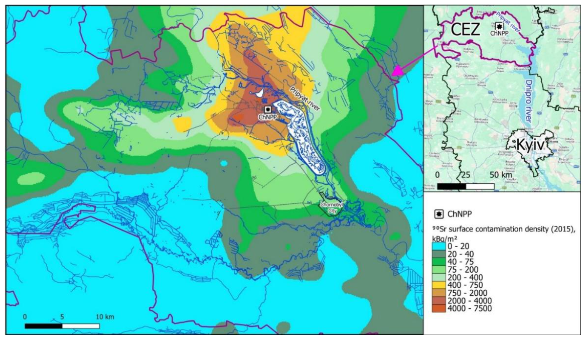
Figure 2.
Conceptual diagram of the framework for assessing groundwater contamination risk from 90Sr in the CEZ using machine-learning methods.
Figure 2.
Conceptual diagram of the framework for assessing groundwater contamination risk from 90Sr in the CEZ using machine-learning methods.
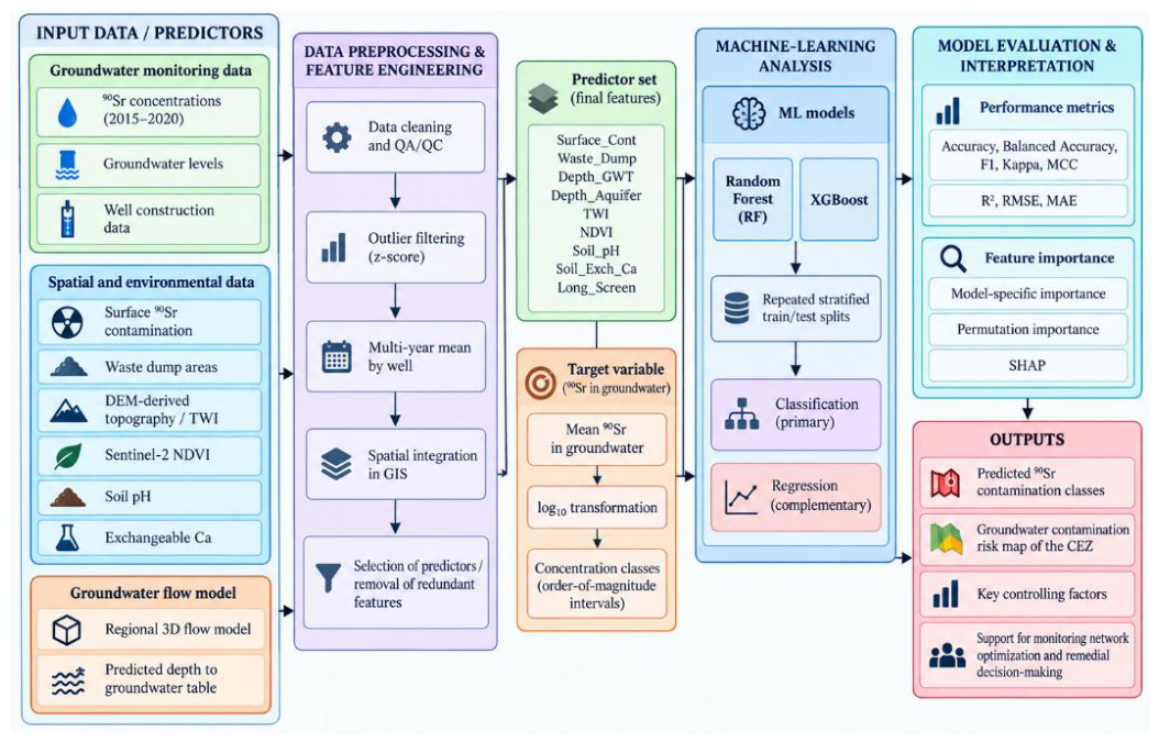
Figure 3.
Mean 90Sr groundwater concentrations for the period 2015-2020 in monitoring wells of the SSE “Ecocenter”.
Figure 3.
Mean 90Sr groundwater concentrations for the period 2015-2020 in monitoring wells of the SSE “Ecocenter”.
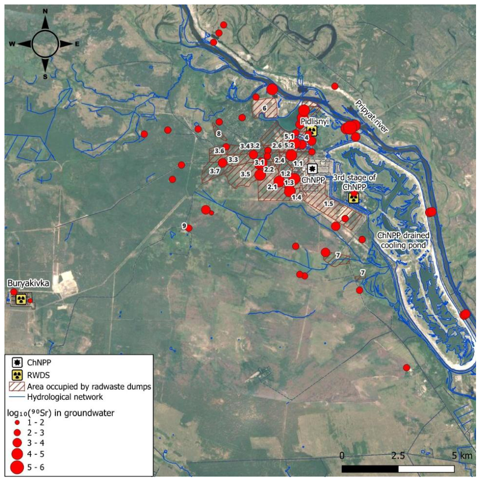
Figure 4.
Distribution of monitoring wells among 90Sr concentration classes.
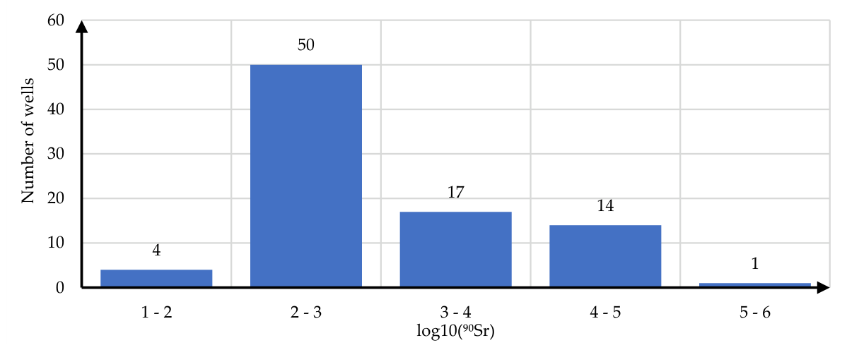
Figure 5.
Equivalent surface contamination densities by 90Sr in waste dump sectors as of 2015 (sector numbers: 1.1-1.4 – Stara Budbaza; 1.5 – Nova Budbaza; 2.1 – 2.6 – Red Forest; 3.1-3.7 – Yanov Station; 5.1 – 5.3 – Neftebaza; 6 – Peschanoe Plato; 7 – Kopachi; 8 – Pripyat).
Figure 5.
Equivalent surface contamination densities by 90Sr in waste dump sectors as of 2015 (sector numbers: 1.1-1.4 – Stara Budbaza; 1.5 – Nova Budbaza; 2.1 – 2.6 – Red Forest; 3.1-3.7 – Yanov Station; 5.1 – 5.3 – Neftebaza; 6 – Peschanoe Plato; 7 – Kopachi; 8 – Pripyat).
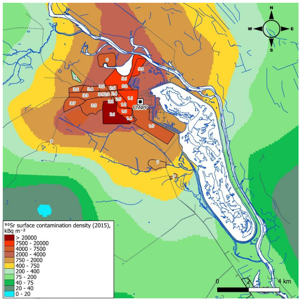
Figure 6.
Spatial distributions of predictor parameters in the study area: (a) topographic wetness index (TWI); (b) normalized difference vegetation index (NDVI); (c) soil pH; (d) soil exchangeable calcium (Ca2+);.
Figure 6.
Spatial distributions of predictor parameters in the study area: (a) topographic wetness index (TWI); (b) normalized difference vegetation index (NDVI); (c) soil pH; (d) soil exchangeable calcium (Ca2+);.
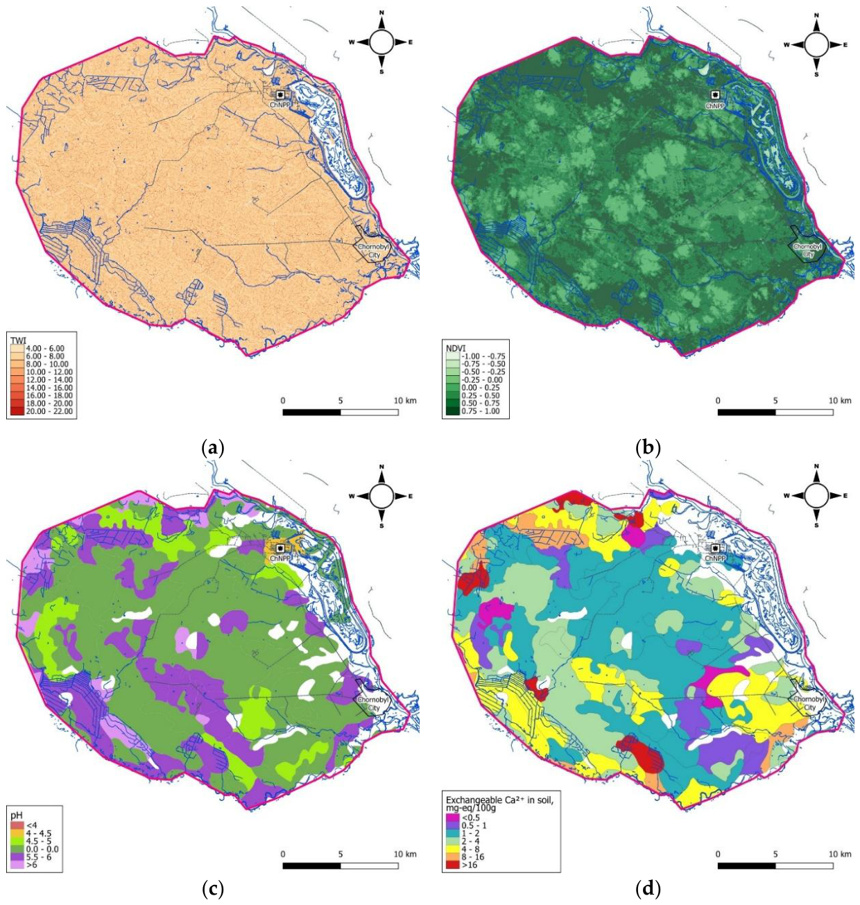
Figure 7.
Groundwater-flow modelling results: (a) predicted groundwater-table depth in the study area; (b) predicted groundwater-level distribution in the unconfined aquifer; and (c) comparison of predicted and observed groundwater levels used for model calibration.
Figure 7.
Groundwater-flow modelling results: (a) predicted groundwater-table depth in the study area; (b) predicted groundwater-level distribution in the unconfined aquifer; and (c) comparison of predicted and observed groundwater levels used for model calibration.
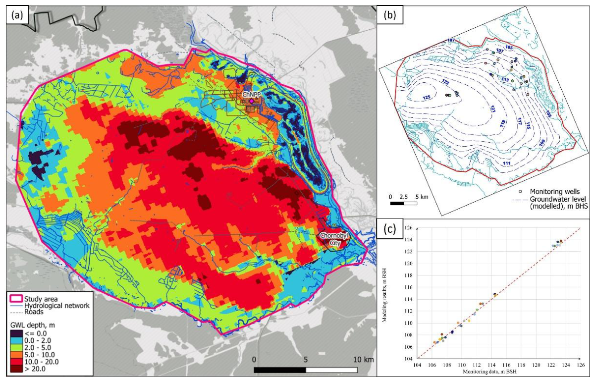
Figure 8.
ML models prediction errors in classifier mode: (a) RF, (b) XGB.
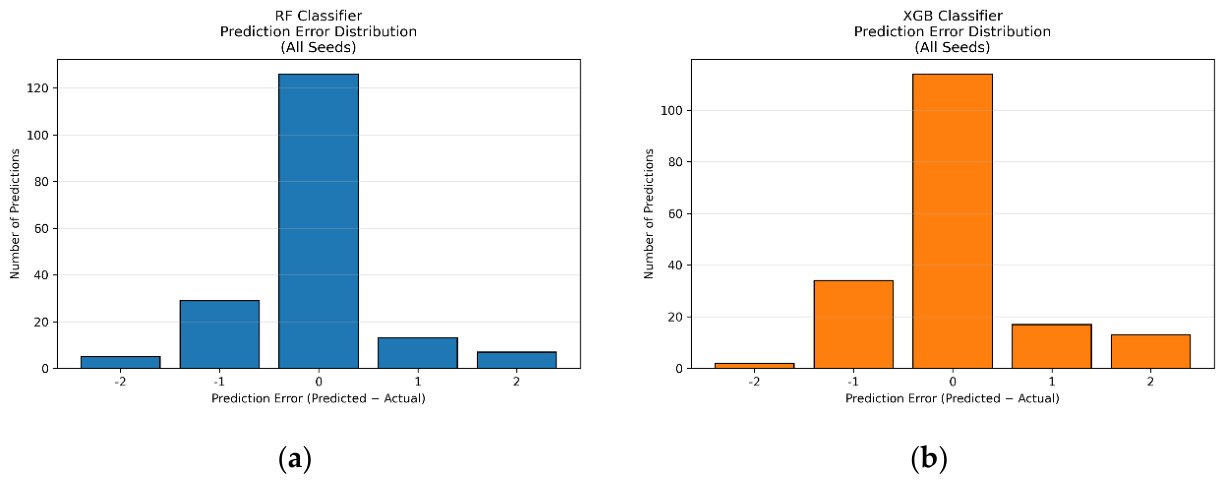
Figure 9.
ML models performance in regressor mode: (a) RF, (b) XGB.
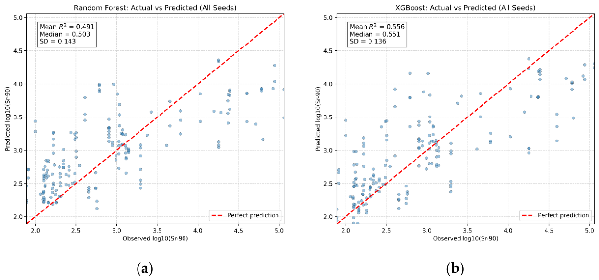
Figure 10.
Feature importance of predictors for the RF and XGB classifiers: (a) model-specific feature importance, (b) permutation importance, and (c) SHAP-based feature importance.
Figure 10.
Feature importance of predictors for the RF and XGB classifiers: (a) model-specific feature importance, (b) permutation importance, and (c) SHAP-based feature importance.
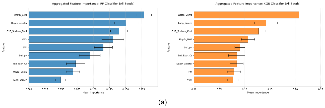
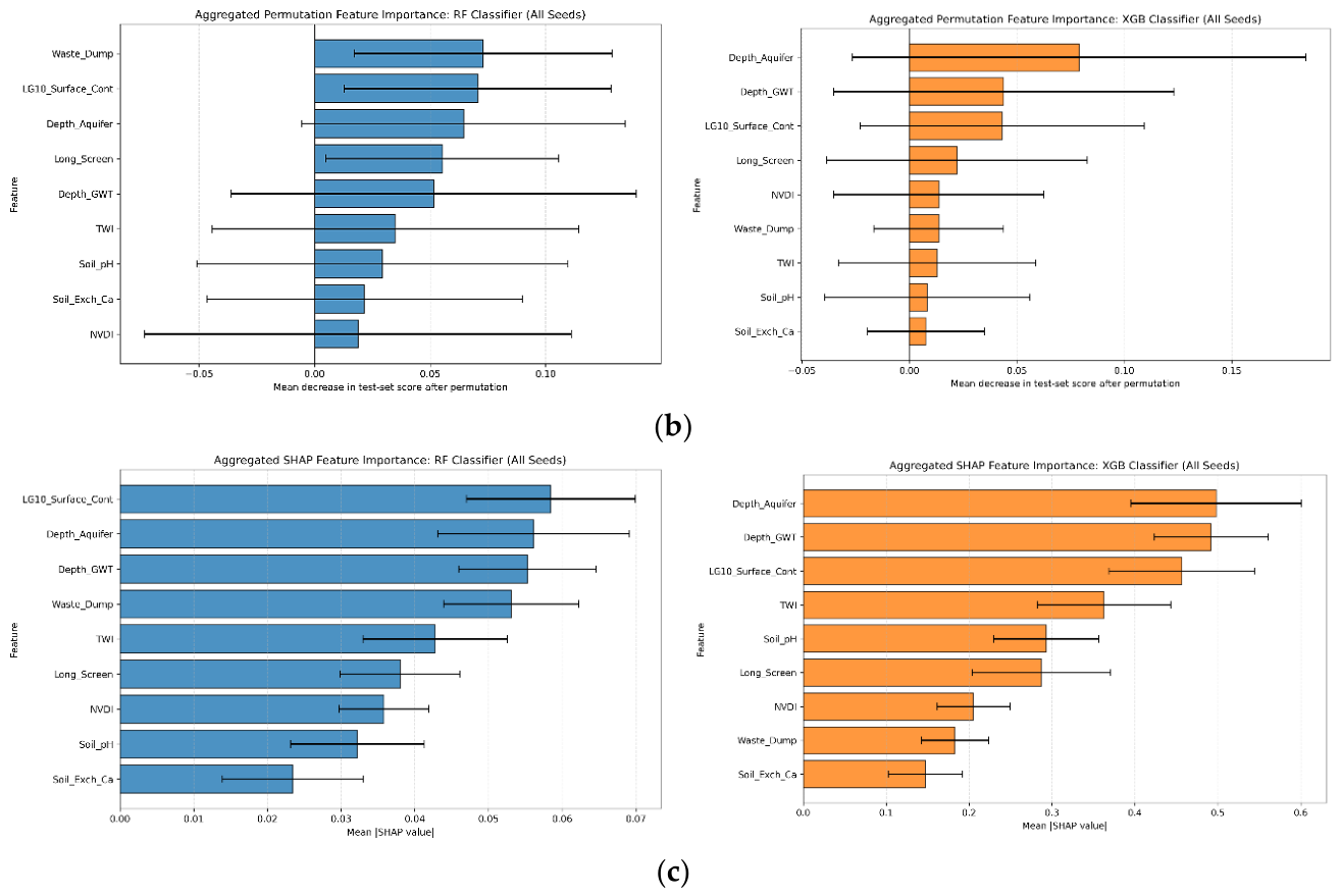
Figure 11.
Spatial distribution of predicted ⁹⁰Sr groundwater contamination classes across the Chornobyl Exclusion Zone obtained using (a) the RF classifier and (b) the XGBoost classifier.
Figure 11.
Spatial distribution of predicted ⁹⁰Sr groundwater contamination classes across the Chornobyl Exclusion Zone obtained using (a) the RF classifier and (b) the XGBoost classifier.
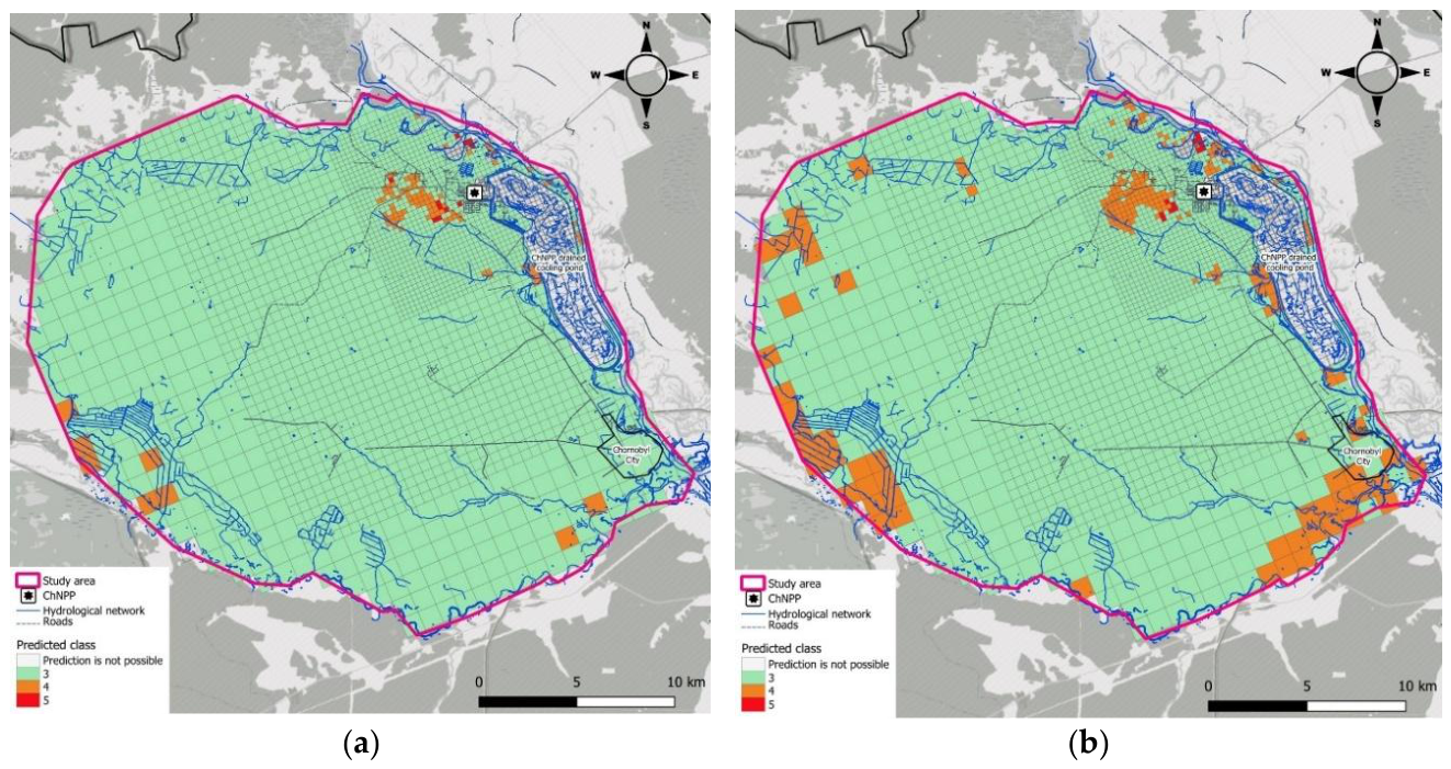
Figure 12.
Spatial distribution of predicted 90Sr groundwater contamination classes in the Chornobyl Nuclear Power Plant near-field area obtained using (a) the RF classifier and (b) the XGBoost classifier.
Figure 12.
Spatial distribution of predicted 90Sr groundwater contamination classes in the Chornobyl Nuclear Power Plant near-field area obtained using (a) the RF classifier and (b) the XGBoost classifier.
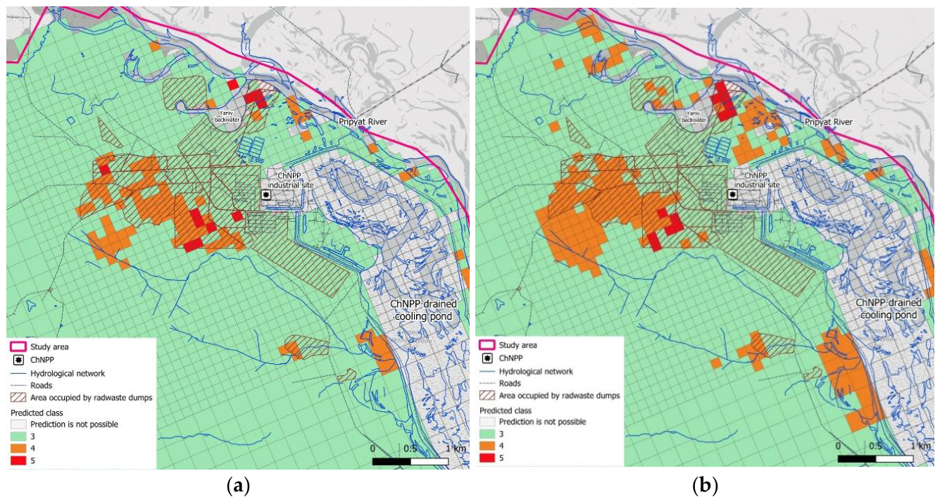

Table 1.
Predictor variables used in machine learning analyses.
| Predictor ID | Full name | Rationale for predictor |
| Source-term characteristics | ||
| Surface_Cont | Surface contamination density by 90Sr | Represents the spatially distributed source term for downward migration of 90Sr from contaminated topsoil to groundwater. |
| Waste_Dump | Location within a radioactive-waste dump area (binary parameter) | Accounts for specific source conditions at radioactive-waste dump sites, where contaminated material is buried in shallow trenches or mounds and may occur substantially closer to the groundwater table than surface fallout contamination. |
| Hydrogeological and groundwater-transport conditions | ||
| Depth_GWT | Depth to groundwater table (multi-year mean) | Controls the thickness of the unsaturated zone through which 90Sr released from near-surface sources must migrate before reaching groundwater. Greater depth generally provides a longer transport pathway and greater potential for retardation and attenuation. This factor is analogous to the “Depth to water” parameter in the DRASTIC methodology. |
| Depth_Aquifer | Depth from the groundwater table to the top of the well screen | Represents the vertical position of the sampled interval within the aquifer. Deeper screened intervals are expected, in general, to have a lower probability of contamination from near-surface sources because of the longer vertical transport pathway and commonly observed decrease of 90Sr concentrations with depth. |
| Topographic and vegetation characteristics | ||
| TWI | Topographical Wetness Index | Characterizes topographically controlled potential for water accumulation and focused infiltration. Higher TWI values may indicate locations with enhanced soil moisture and recharge, which can facilitate downward migration of 90Sr from the surface. The predictor is conceptually related to the recharge and topography components of DRASTIC. |
| NDVI | Normalized Difference Vegetation Index | Provides a proxy for vegetation density and biomass. Vegetation can influence ⁹⁰Sr redistribution through biological recycling, potentially retaining and redistributing ⁹⁰Sr within the rooting zone and thereby modifying its availability for downward migration. |
| Geochemical factors | ||
| Soil_pH | Soil pH | Influences the dissolution rate of Chornobyl fuel particles containing 90Sr. More acidic conditions generally enhance dissolution of the uranium-oxide fuel-particle matrix and therefore increase release of ⁹⁰Sr into mobile forms. |
| Soil_Exch_Ca | Exchangeable Ca content in topsoil | Provides an indicator of soil ion-exchange properties relevant to 90Sr retention. Exchangeable Ca is associated with the cation-exchange complex and can also compete with Sr²⁺ for sorption sites, thereby influencing the mobility and retardation of 90Sr in soil. |
| Monitoring-well characteristics | ||
| Long_Screen | Monitoring-well screen length category (short/long; binary parameter) | Accounts for differences in sampled vertical interval. Wells with long screens integrate groundwater over a larger part of the aquifer thickness and may therefore yield depth-averaged 90Sr concentrations lower than those observed in shallow, short-screen wells where contamination is commonly greatest. |
Table 2.
Performance of RF and XGB models across 10 independent runs.
| Metric | Mean | Median | SD | 95% CI half-width |
| RF Classifier | ||||
| Accuracy | 0.70 | 0.72 | 0.09 | 0.06 |
| Balanced Accuracy | 0.60 | 0.62 | 0.13 | 0.09 |
| Kappa (Cohen’s Kappa) | 0.42 | 0.49 | 0.16 | 0.12 |
| MCC (Matthews Correlation Coefficient) | 0.45 | 0.51 | 0.17 | 0.12 |
| F1 Score | 0.66 | 0.68 | 0.09 | 0.07 |
| XGB Classifier | ||||
| Accuracy | 0.64 | 0.64 | 0.08 | 0.06 |
| Balanced Accuracy | 0.57 | 0.56 | 0.10 | 0.07 |
| Kappa (Cohen’s Kappa) | 0.34 | 0.34 | 0.15 | 0.11 |
| MCC (Matthews Correlation Coefficient) | 0.35 | 0.35 | 0.15 | 0.11 |
| F1 Score | 0.62 | 0.61 | 0.09 | 0.06 |
| RF Regressor | ||||
| R² (Coefficient of Determination) | 0.50 | 0.53 | 0.15 | 0.11 |
| RMSE (Root Mean Square Error) | 0.58 | 0.57 | 0.08 | 0.06 |
| MAE (Mean Absolute Error) | 0.47 | 0.46 | 0.06 | 0.04 |
| XGB Regressor | ||||
| R² (Coefficient of Determination) | 0.55 | 0.54 | 0.15 | 0.11 |
| RMSE (Root Mean Square Error) | 0.55 | 0.57 | 0.09 | 0.07 |
| MAE (Mean Absolute Error) | 0.42 | 0.43 | 0.08 | 0.05 |
Disclaimer/Publisher’s Note: The statements, opinions and data contained in all publications are solely those of the individual author(s) and contributor(s) and not of MDPI and/or the editor(s). MDPI and/or the editor(s) disclaim responsibility for any injury to people or property resulting from any ideas, methods, instructions or products referred to in the content. |
© 2026 by the authors. Licensee MDPI, Basel, Switzerland. This article is an open access article distributed under the terms and conditions of the Creative Commons Attribution (CC BY) license.
Copyright: This open access article is published under a Creative Commons CC BY 4.0 license, which permit the free download, distribution, and reuse, provided that the author and preprint are cited in any reuse.