

Submitted:
25 September 2026
Posted:
28 September 2026
You are already at the latest version
Abstract
Hourly forecasting of electricity load is a very important problem from the practical point of view, due to the mostly big spread on one-day energy markets. Many models have been proposed in the literature. Our idea is to combine five individual models through multiple regression estimated on last 48 hours of the demand time series. The individual models are: multiple regression with dummy variables coding week days and hours, ARIMA, exponential smoothing, support vector regression, and artificial neural regression. Residuals of these models were later analysed by ARIMA. The basic harmonic in time series was equal to 168 (7 days x 24 hours). Individual models theoretical values in last 48 hours were used to estimate regression model combining individual models. The combined model fitted the data considerably better in-sample, and its 48-hour forecast error was slightly lower than for the individual models (MAPE 3.57% vs 3.65–4.44%). The paper proposed some kind of framework for practical use based on rolling data, each day adding the latest 24-hour data, and eliminating 24 oldest observations. The structure of individual models can be kept constant, at least for some months.
Keywords:
electricity load forecasting
; multiple regression
; ARIMA
; exponential smoothing
; support vector regression
; artificial neural networks
1. Introduction
Planning the generation (supply) of energy on the market, regardless of its scope, requires demand forecasts. Forecasting the electricity load is the subject of many research in literature. In the energy market, regardless of the perspective (long-term, e.g. annual, or short-term, e.g. hourly or daily), forecasting the demand for electricity is of key importance – it also requires different approaches depending on the forecast horizon. The forecasting methods proposed in the literature use different types of data, including historical data, which are characterized by cyclical behaviour and trends, which supports the assumption that demand will follow a similar pattern. The specificity of this market – the stochastic nature of electricity demand, together with parameters such as weather conditions (including temperature, humidity, wind speed, cloud cover), time of day or day of the week (holidays, mass events) and work mode – affect deviations from the expected demand. Forecasting the demand for electricity is important, among other things, in capacity and transmission planning, generation planning and also in pricing. For capacity planning, it is necessary to make a long-term estimate of the total demand as a function of economic parameters and those resulting from demographic conditions, while short-term (hourly) estimates allow for improving the efficiency of day-ahead markets.
The importance of forecasting in the energy market is crucial. Review studies are available in the literature on the subject. Reviews are carried out of methods for long-term electric load forecasting [1], methods, determinants, and policy implications of forecasting electricity demand [2], electrical load forecasting models [3], electricity demand forecasting techniques [4], energy models for demand forecasting [5]. A detailed analysis of the literature on forecasting methods is presented in [6]. In addition, a review of research in the field of energy price forecasting was carried out by [7], highlighting the complexity of the available solutions, their strengths and weaknesses, and the opportunities and threats associated with forecasting tools. Hong and Fan [8] reviewed issues related to probabilistic forecasting of electricity demand, covering the most important techniques, methodologies and assessment methods. They also pointed to the need for further research, including the development of repeatable case studies, the improvement of methods for assessing and valuing probabilistic forecasts, and the consideration of new technologies and energy policy in the probabilistic forecasting process.
The issue of territory plays an important role in forecasting electricity demand. Forecasts may concern areas of varying scope (diversity), as well as facilities with different characteristics. Below is a list of selected studies that concern the area, among others:
1/ Countries, including, for example: Italy [9,10], Jordan [11], Spain [12], China [13,14], Turkey [2,6,15,16], Australia [17].
3/ Larger areas, such as Europe [21], selected EU countries (Austria, Germany, Spain, France, Italy, Great Britain) and US states (Florida, New York, California) [22] , groups of countries: Poland, France, Germany, Great Britain, Turkey and the Scandinavian countries [23], Great Britain and France [24].
4/ Smaller territories, such as local areas in Denmark [25], Prague in the Czech Republic [26], and the Green Energy Park in Morocco [27].
Due to the specific nature of the energy market, hourly forecasts are developed [15,23,24,31,32,33], as well as forecasts of daily demand [16,17,18,27,34,35,36,37], and forecasts for longer periods, e.g., weekly [23], monthly [28,38,39], or annual [23,40]. Numerous research methods and approaches are employed to develop these forecasts.
In studies concerning the assessment of demand and load (electric load forecasting), a wide variety of forecasting methods are used, including:
• seasonal hybrid procedure [13];
• particle swarm optimization [41];
• modelling – SARIMAX with interactions [33], application of residual modification approach in seasonal ARIMA [14], a semi-parametric additive model [42], Generalized Additive Model (GAM) [17], hybrid RSVMG model (recurrent support vector machines with genetic algorithms) [19], an adaptive neural-wavelet model [43];
• a model based on support vector regression with differential evolution algorithm [40];
• using double seasonal exponential smoothing [44];
• expands double-seasonal methods – specifically double seasonal ARMA and adaptations of Holt-Winters exponential smoothing – to handle the triple-seasonality structure [45];
• with exponentially weighted methods – compares exponential smoothing formulations, discount weighted regression, cubic splines, and singular value decomposition (SVD) [24];
• spectral analysis using the fast Fourier transform (FFT) [23];
• integration of artificial neural networks and genetic algorithm [46].
In their study, Vilar, Cao, and Aneiros [35] used a functional approach (FDA), in which the entire curve of the variable during the day (demand or price) is treated as a single functional observation, as well as non-parametric and semi-parametric models, in which non-linear functional autoregression and semi-functional partial linear (SFPL) models were used.
In forecasting electricity demand, the potential benefits of using numerical weather forecasting models are also assessed [9], as are the impact of calendar effects and the detail of the forecast [29], periodic variations and demand segregation [6], and the assessment of demand by breaking down the aggregated (total) electricity demand into components such as heating, cooling, lighting and industrial activity [23]. To predict electricity consumption, the following are used, among others: Multi-Scale Graph Attention Network Based on Encoding Decomposition [47].
The multitude of methods used allows researchers to perform comparative analyses, including, for example, the comparative analysis of Kolmogorov-Arnold and recurrent neural networks for day-ahead photovoltaic forecasting [27]. The effectiveness of the DCNN architecture was compared with other machine learning models and recurrent networks (RNN, ELM), demonstrating higher accuracy and effectiveness in mapping nonlinear dependencies in the data [18].
Various factors influencing demand are also assessed, such as holiday periods [48] and meteorological variables [17,39].
There are also studies on forecasting demand/consumption/management in the field of energy from renewable sources [49,50,51].
The aim of this paper is to propose the model for hourly electricity load forecasting using the combination of five separate models: regression analysis, ARIMA, exponential smoothing, support vector regression and artificial neural networks. In the final step, forecasts from these models are combined through the multiple regression.
Calculations presented in this paper were performed using STATISTICA ver. 13, Optuna library, and Python (scikit-learn).
2. Materials and Methods
The process of short term forecasting the electricity load heavily depends on the organization of the order system in a given company. Our data comes from the area in the southern Poland. A certain number, unknown to us, was added to all values making the data anonymous. In the company which owns the real data, staff starts work at 6 a.m. The available data covers the period until last midnight. The staff has to order electricity for the next day until 11 a.m. It means that the forecasting system should provide predictions for the next 48 hours, starting midnight. Practically prediction for 25-48 hours are really important since the load for the current day has been ordered the day before. We assume that weather forecast for the day ahead is available.
Models, results and propositions are based on many exercises, different versions and also different data. What we proposed here is somehow the final results of our investigations.
The learning set of hourly data is a rolling one. Each day new 24 observations are added, and the oldest 24 are removed, so the learning set has always the same length. The following individual models are estimated on the same learning set:
- multiple regression plus ARIMA of residuals (MR+ARIMA);
- ARIMA;
- Exponential Smoothing (ES)+ARIMA;
- Support Vector Regression (SVR)+ARIMA;
- Artificial Neural Network (NN)+ARIMA.
In the first part of the analysis, structures of the individual models are established. They are unchanged in time, during the rolling process. This assumption has been validated through our analyses, but of course these structures should not be stable forever. It is difficult to advise how often the model structure should be checked. It heavily depends on individual cases – areas, seasons of the year, and maybe some other factors.
MR+ARIMA
This approach has two steps. In the first one, multiple regression model is estimated, and in the second one, residuals are checked. If they are not purely random, then the ARIMA model is fitted to them. The final theoretical values and forecasts are calculated as sum of MR and ARIMA (if estimated).
The list of explaining variables in multiple regression models consists of one measurable external variable – average daily temperature and dummy variables identifying the day of the week and the hour of the day. Dummy variables are coded as 0/1. There are 6 variables for week days and 23 variables for hours. The missing ones – baselines – represents the minimum load. There is one more dummy variable identifying local holidays which comes not on Sundays – like Christmas, National Holidays, bank holidays all others of this type. Possible trend is covered by variable t. Multiple regression model is estimated by Ordinary Least Squares method. ARIMA of residuals is identified, estimated and verified in a classical way as described in the next paragraph.
ARIMA
Autoregressive Integrated Moving Average (ARIMA) models are widely used in the analysis and forecasting of different types of time series, including the ones with trend and seasonality. Electricity load time series always have a short-period seasonal component and usually no trend. The model which is used in this paper is sometimes called SARIMA, as Seasonal ARIMA (Just ARIMA is used in STATISTICA software). No matter which notation is used, the model has two components – nonseasonal and seasonal. It is defined in two brackets as ARIMA(p,d,q)(Ps,Ds,Qs), where:
- p – order of autoregression;
- d – number of first order differencing;
- q – order of moving average;
- s – seasonal period;
- Ps – order of seasonal autoregression;
- Ds – number of seasonal differencing;
- Qs – order of seasonal moving average.
In classical approach orders of autoregression and moving average are identified through the analysis of autocorrelation function and partial autocorrelation function. Nowadays, first the possible trend and seasonality are removed by differencing, and then p and q (usually rather small) are “guessed” checking p-values of possible models. If autoregression of residuals shows that seasonality was not completely removed, we make Ps and Qs active.
Exponential Smoothing+ARIMA
Exponential Smoothing is using past values of the time series with weights decreasing exponentially over time. In the classical form the current smoothed value is a weighted average (steered by parameter α) of the current observed value and the previous smoothed value. In our study the model has an additional parameters δ which decides the importance of past values from the seasonal period, and γ is smoothing parameter for the possible trend. Parameters are estimated tracking all values with step 0.001, and measuring the goodness-of-fit with variance of residuals.
SVR+ARIMA
Support Vector Regression fits a regression type function to the explained (dependent) variable, allowing a margin of tolerance around this function. Errors that fall within that margin don’t count. The following parameters must be estimated:
- ε (epsilon) – defines the width of the tolerance margin around the fitted function;
- C – controls how much SVR penalizes errors on points outside the tube;
- kernel – determines how SVR handles nonlinear pattern. The practical choice is between RBF (Radial Basis Function) or polynomial kernel;
- γ (gamma) – a hyperparameter that defines how far the influence of a training example reaches. It can be seen as the inverse of the radius of influence of samples selected by the model as support vectors.
Artificial Neural Networks+ARIMA
A Multilayer Perceptron (MLP) has been chosen for our model as an artificial neural network. It is composed of fully connected layers with nonlinear activation functions. In our model the input layer receives the same features that are used in multiple regression and passes them forward. In hidden intermediate layers neurons computed sums of input, add biases, and apply nonlinear activation functions. Output layer calculates the final prediction based on the information from the final hidden layer. ReLU (rectified linear unit) was used as an activation function, and Limited-memory BFGS (L-BFGS) as optimization algorithm. Hyperparameter alpha sets the regularization power in L2, and tol defines the threshold below which, changes in objective function are so small that optimization process is terminated.
General flowchart of the proposed model is shown on Figure 1.
3. Results
The learning set in our example covers 84 days, which are 12 weeks or 2016 hours. The data is presented on Figure 2.
On Figure 2 we can clearly identify weeks and days. Typical seasonalities are present in load time series, no matter what is covered by the data. Weekly average profile of our data is presented in Figure 3.
The lowest demand for electricity was – as expected – on Sundays, so we take Sunday as base variant for dummy coding of week days. The daily profile is presented on Figure 4.
Most of the clients in the analysed area are households, what explains the highest demand for electricity between 4-11 p.m., when people are back home from offices, factories and schools. As the base for within-day hour coding we took the hour number 3, the third hour in a day.
3.1. Multiple Regression with Residual ARIMA
The basic multiple regression model for electricity load learning set is presented in Table 1. The month can be of course identified from the date, but the average daily temperature better identifies the season within the year.
Even non-significant variables marking hours have been left in the model to secure the full daily profile of the load. Residuals from the regression model are modelled (See Table 2) by ARIMA(1,0,1)(0,1,1) with seasonal period s=168.
3.2. ARIMA
Single non-seasonal differencing and single seasonal differencing with s=168 were the elements of transforming the original time series into a stationary one. ARIMA model was in the form of ARIMA(1,1,3)(1,1,1) – Table 3.
It is obvious that we did not try to estimate another ARIMA for the residuals of basic ARIMA model.
3.3. Exponential Smoothing
Automatic search has found that parameters of exponential smoothing model are equal to: alpha=1.000, delta=1.000, and gamma=0.000, which is in fact a naïve model. ARIMA model for exponential smoothing residuals is described in Table 4. Coefficients are very close to ARIMA for original series.
3.4. Support Vector Regression
In search for optimal hyperparameters of SVR, an Optuna library has been used (optuna.org). Each configuration has been verified by 10-folded cross-validation on learning set, and rated by Root Mean Square Error (RMSE). After 200 runs, the best SVR model used polynomial kernel with degree 2, and other parameters equal to:
- C = 805.224
- epsilon = 5.083
- gamma = 0.0890
- coef0 = 1.586
3.5. Artificial Neural Network
30 NN configurations were considered in the first experiment, with one or two hidden layers, 8 to 128 neurons in the first layer, and four activation functions. The simplest networks with just one hidden layer gave the best results. So in the second experiment, there were just one layer with 2 to 16 neurons. Finally, the best network had 7 neurons, ReLU was taken as activation function. Parameters were equal to:
- alpha = 6.20 x 10⁻⁶
- tol = 3.01 x 10⁻⁵
3.6. Combining individual models
The combining data set consists of 48 hours prior to the forecasting period. Multiple regression model is estimated on this data. The observed electricity demand within these 48 hours is an explained variable, and theoretical values from five individual models are explaining (independent variables). This is the way how singles models are combined for the regression model which is used for the final forecast. Multiple regression model for our example is presented in Table 5.
Mean Absolute Percentage Errors for the 48 hour forecasts calculated by individual models and the final one are given in Table 6.
4. Discussion
Hourly forecasting of electricity load is important mostly from practical point of view. Companies which sale electricity rely on long-term agreements which should be adjusted on short time basis. They can buy or sale electricity in exchange platforms but the spread of prices can be substantial. Bosses of companies would like to have the forecasting error less than 1% which is almost impossible to achieve, even in normal circumstances, without strange weather events.
It is easier to forecast if the data cover more or less homogeneous region. On industrial areas, we can expect bigger drops in demand during weekends or national holidays, when factories are closed. In residential areas this effect is much smaller. We know, from our experience, that big factories (like ironworks) are usually billed separately.
Our methodological proposition is similar to bagging and boosting procedures, but there are some important differences. In classical bagging, models are trained on different bootstrap samples obtained through sampling with replacement. Our individual models are estimated using the same time series data. Boosting trains models sequentially (one after another), where each new model tries to fix the errors of the previous one. In our approach, residuals from individual models are modelled by ARIMA – of course except ARIMA model itself.
The choice and the number of individual models can always be discussed. We took models which are relatively popular in subject literature and also been used by us in other applications. Models are combined with multiple regression in which we rely not only on statistical significance but rather on goodness-of-fit. In terms of MAPE the combined model is slightly better than individual ones (Table 6). The idea is, that individual models can capture different aspects of time series variability and contribute to the combined model. The in-sample MAPE of the combined model is optimistic, since its parameters are estimated on the same 48 observations; the forecasting period gives the fair comparison.
Author Contributions
Conceptualization, A.S., G.M., M.M. and J.W.; methodology, A.S., and G.M.; software, A.S. and G.M.; validation, M.M. and J.W.; formal analysis, A.S. G.M. and M.M.; investigation, M.M.; resources, J.W..; data curation, A.S and M.M; writing—original draft preparation, A.S.; writing—review and editing, A.S. and M.M.; visualization, G.M.; supervision, M.M. and J.W.; project administration, A.S.; funding acquisition, J.W. All authors have read and agreed to the published version of the manuscript.
Funding
This research received no external funding
Data Availability Statement
Our research data can be obtained from the authors
Conflicts of Interest
The authors declare no conflicts of interest
Abbreviations
The following abbreviations are used in this manuscript:
| ARIMA | Autoregressive Integrated Moving Average |
| SARIMA | Seasonal Autoregressive Integrated Moving Average |
| CNN | Convolutional Neural Networks |
| SARIMAX | Seasonal Autoregressive Integrated Moving Average with Exogenous Variables |
| GAM | General Additive Model |
| RSVMG | Recurrent Support Vector Machines with Genetic algorithms |
| SVD | Singular Value Decomposition |
| FFT | Fast Fourier Transform |
| FDA | Functional Data Analysis |
| SFPL | Semi-functional Partial Linear models |
| DCNN | Deep Convolutional Neural Networks |
| ELM | Extreme Learning Machines |
| MR | Multiple Regression |
| ES | Exponential Smoothing |
| SVR | Support Vector Regression |
| NN | Neural Networks |
| RuLU | Rectified Linear Unit |
| L-BFGS | Limited-memory Broyden-Fletcher-Goldfarb-Shanno algorithm |
References
- Aditya, T.; Jaipuria, S.; Kumar Dadabada, P. A Review of Methods for Long-Term Electric Load Forecasting. J. Forecast. 2025, 44, 1403–1423. [Google Scholar] [CrossRef]
- Elbaş, H.; Bilgin, T.T. Forecasting electricity demand in Türkiye: A comprehensive review of methods, determinants, and policy implications. J. Energy Syst. 2025, 9.1, 132–158. [Google Scholar] [CrossRef]
- Kuster, C.; Rezgui, Y.; Mourshed, M. Electrical load forecasting models: A critical systematic review. Sustain. Cities Soc. 2017, 35, 257–270. [Google Scholar] [CrossRef]
- Singh, A.K.; Khatoon, I.S. An overview of electricity demand forecasting techniques. National Conference on Emerging Trends in Electrical, Instrumentation and Communication Engineering 2013, 3(3), 38-48.
- Suganthi, L.; Samuel, A.A. Energy models for demand forecasting-a review. Renew. Sustain. Energy Rev. 2012, 16, 1223–1240. [Google Scholar] [CrossRef]
- Yukseltan, E.; Yucekaya, A.; Bilge, A.H. Forecasting electricity demand for Turkey: Modeling periodic variations and demand segregation. Appl. Energy 2017, 193, 287–296. [Google Scholar] [CrossRef]
- Weron, R. Electricity price forecasting: A review of the state-of-the-art with a look into the future. Int. J. Forecast. 2014, 30, 1030–1081. [Google Scholar] [CrossRef]
- Hong, T.; Fan, S. Probabilistic electric load forecasting: A tutorial review. Int. J. Forecast. 2016, 32, 914–938. [Google Scholar] [CrossRef]
- De Felice, M.; Alessandri, A.; Ruti, P.M. Electricity demand forecasting over Italy: Potential benefits using numerical weather prediction models. Electr. Power Syst. Res. 2013, 104, 71–79. [Google Scholar] [CrossRef]
- Ghiani, E.; Galici, M.; Mureddu, M.; Pilo, F. Impact on electricity consumption and market pricing of energy and ancillary services during pandemic of COVID-19 in Italy. Energies 2020, 13, 3357. [Google Scholar] [CrossRef]
- Momani, M.A. Factors affecting electricity demand in Jordan. Energy Power Eng. 2013, 5, 50–58. [Google Scholar]
- Santiago, I.; Moreno-Munoz, A.; Quintero-Jiménez, P.; Garcia-Torres, F.; Gonzalez-Redondo, M.J. Electricity demand during pandemic times: The case of the COVID-19 in Spain. Energy Policy 2021, 148(A), 111964. [Google Scholar] [CrossRef] [PubMed]
- Zhu, S.; Wang, J.; Zhao, W.; Wang, J. A seasonal hybrid procedure for electricity demand forecasting in China. Appl. Energy 2011, 88, 3807–3815. [Google Scholar] [CrossRef]
- Wang, Y.; Wang, J.; Zhao, G.; Dong, Y. Application of residual modification approach in seasonal ARIMA for electricity demand forecasting: A case study of China. Energy Policy 2012, 48, 284–294. [Google Scholar] [CrossRef]
- Yukseltan, E.; Yucekaya, A.; Bilge, A.H. Hourly electricity demand forecasting using Fourier analysis with feedback. Energy Strategy Rev. 2020, 31, 100524. [Google Scholar] [CrossRef]
- Yukseltan, E.; Kok, A.; Yucekaya, A.; Bilge, A.H.; Agca Aktunc, E.; Hekimoğlu, M. The Impact of COVID-19 Pandemic and Restrictions on the Electricity Demand and Daily Demand Curve in Turkey, Working Paper 2021. Paris, France: International Energy Agency. Paris, France.
- McCulloch, J.; Ignatieva, K. Forecasting high frequency intra-day electricity demand using temperature. SSRN Electr. J. 2017. [Google Scholar] [CrossRef]
- Khan, S.; N. Javaid, A.; Chand, A.B.M.; Khan, F.; Rashid, I.U.; Afridi, I.U. Electricity load forecasting for each day of week using deep CNN, in: Workshops of the International Conference on Advanced Information Networking and Applications, 2019, Springer, Cham.
- Pai, P.F.; Hong, W.C. Forecasting regional electricity load based on recurrent support vector machines with genetic algorithms. Electr. Power Syst. Res. 2005, 74, 417–425. [Google Scholar] [CrossRef]
- Taylor, J.W.; Bizza, R. Using weather ensemble predictions in electricity demand forecasting. Int. J. Forecast. 2003, 19, 57–70. [Google Scholar] [CrossRef]
- Bahmanyar, A.; Estebsari, A.; Ernst, D. The impact of different COVID-19 containment measures on electricity consumption in Europe. Energy Res. Soc. Sci. 2020, 68, 101683. [Google Scholar] [CrossRef] [PubMed]
- Prol, L.J.; Sungmin, O. Impact of COVID-19 Measures on Short-term Electricity Consumption in the Most Affected EU Countries and USA States. iScience 2020, 23, 101639. [Google Scholar] [CrossRef] [PubMed]
- Yucekaya, A.; Bilge, A.H.; Yukseltan, E.; Aktunc, E.A. Segregation of Hourly Electricity Consumption: Quantification of Demand Types Using Fourier Transform. Int. J. Energy Econ. Policy 2025, 15, 384–396. [Google Scholar] [CrossRef]
- Taylor, J.W. Short-term load forecasting with exponentially weighted methods. IEEE Trans. Power Syst. 2012, 27, 458–464. [Google Scholar] [CrossRef]
- Andersen, F.M.; Larsen, H.V.; Gaardestrup, R.B. Long term forecasting of hourly electricity consumption in local areas in Denmark. Appl. Energy 2013, 110, 147–162. [Google Scholar] [CrossRef]
- Bašta, M.; Helman, K. Scale-specific importance of weather variables for explanation of variations of electricity consumption: the case of Prague, Czech Republic. Energy Econ. 2013, 40, 503–514. [Google Scholar] [CrossRef]
- Mouna, E.-Q.; Hicham, O.; Mohamed, L.; Ahmed, A.; Abdelilah, R.; Lahoucine, I.-K. Comparative analysis of Kolmogorov–Arnold and recurrent neural networks for day-ahead photovoltaic forecasting with Metaheuristic optimization for cost and battery management at Green Energy Park, Morocco. Results Eng. 2025, 108203. [Google Scholar] [CrossRef]
- Islam, S.M.; Al-Alawi, S.M.; Ellithy, K.A. Forecasting monthly electric load and energy for a fast growing utility using an artificial neural network. Electr. Power Syst. Res. 1995, 34, 1–9. [Google Scholar] [CrossRef]
- Lusis, P.; Khalilpour, K.R.; Andrew, L.; Liebman, A. Short-term residential load forecasting: Impact of calendar effects and forecast granularity. Appl. Energy 2017, 205, 654–669. [Google Scholar] [CrossRef]
- Prabhat, P.; Rijal, H.B.; Yoshida, K. Development of a statistical model for long-term electricity forecasting in residential buildings. Energy Build. 2026, 117972. [Google Scholar] [CrossRef]
- Crowley, C.; Joutz, F.L. Hourly Electricity Loads: Temperature Elasticities and Climate Change. United States: 23rd US Association of Energy Economics North American Conference 2003. United States, 2003.
- Filik, Ü.B.; Gerek, Ö.N.; Kurban, M. A novel modeling approach for hourly forecasting of long-term electric energy demand. Energy Convers. Manag. 2011, 52, 199–211. [Google Scholar] [CrossRef]
- Elamin, N.; Fukushige, M. Modeling and forecasting hourly electricity demand by SARIMAX with interactions. Energy 2018, 165 (B), 257–268. [Google Scholar] [CrossRef]
- Conejo, A.J.; Contreras, J.; Espínola, R.; Plazas, M.A. Forecasting electricity prices for a day-ahead pool-based electric energy market. Int. J. Forecast. 2005, 21, 435–462. [Google Scholar] [CrossRef]
- Vilar, J.M.; Cao, R.; Aneiros, G. Forecasting next-day electricity demand and price using nonparametric functional methods. Int. J. Electr. Power Energy Syst. 2012, 39, 48–55. [Google Scholar] [CrossRef]
- Clements, A.E.; Hurn, A.S.; Li, Z. Forecasting day-ahead electricity load using a multiple equation time series approach. Eur. J. Oper. Res. 2016, 251, 522–530. [Google Scholar] [CrossRef]
- Jiang, D.; Guo, Y.; Cao, F.; Xue, J.; Ma, K.; Song, Y. MW-EOT-XG: Volatility-decoupled ensemble learning for enhanced day-ahead electricity price forecasting. Energy Rep. 2026, 109431. [Google Scholar] [CrossRef]
- Hor, C.L.; Watson, S.J.; Majithia, S. Analyzing the impact of weather variables on monthly electricity demand. IEEE Trans. Power Syst. 2005, 20, 2078–2085. [Google Scholar] [CrossRef]
- Apadula, F.; Bassini, A.; Elli, A.; Scapin, S. Relationships between meteorological variables and monthly electricity demand. Appl. Energy 2012, 98, 346–356. [Google Scholar] [CrossRef]
- Wang, J.; Li, L.; Niu, D.; Tan, Z. An annual load forecasting model based on support vector regression with differential evolution algorithm. Appl. Energy 2012, 94, 65–70. [Google Scholar] [CrossRef]
- AlRashidi, M.R.; EL-Naggar, K.M. Long term electric load forecasting based on particle swarm optimization. Appl. Energy 2010, 87, 320–326. [Google Scholar] [CrossRef]
- Fan, S.; Hyndman, R.J. Short-term load forecasting based on a semi-parametric additive model. IEEE Trans. Power Syst. 2012, 27, 134–141. [Google Scholar] [CrossRef]
- Zhang, B.L.; Dong, Z.Y. An adaptive neural-wavelet model for short term load forecasting. Electr. Power Syst. Res. 2001, 59, 121–129. [Google Scholar] [CrossRef]
- Taylor, J.W. Short-term electricity demand forecasting using double seasonal exponential smoothing. J. Oper. Res. Soc. 2003, 54, 799–805. [Google Scholar] [CrossRef]
- Taylor, J.W. Triple seasonal methods for short-term electricity demand forecasting. Eur. J. Oper. Res. 2010, 204, 139–152. [Google Scholar] [CrossRef]
- Azadeh, A.; Ghaderi, S.F.; Tarverdian, S.; Saberi, M. Integration of artificial neural networks and genetic algorithm to predict electrical energy consumption. Appl. Math. Comput. 2007, 186, 1731–1741. [Google Scholar] [CrossRef]
- Huang, S.; Que, H.; Zeng, L.; Yang, J.; Zheng, K. Multi-Scale Graph Attention Network Based on Encoding Decomposition for Electricity Consumption Prediction. Energies 2024, 17, 5813. [Google Scholar] [CrossRef]
- Brubacher, S.; Wilson, G. Interpolating time series with application to the estimation of holiday effects on electricity demand. Appl. Stat. 1976, 25, 107–116. [Google Scholar] [CrossRef]
- Kumar, M.; Sharma, D. Energy Management in Microgrids with Uncertainty in EV and Renewable Sources. Iran. J. Sci. Technol. Trans. Electr. Eng. 2025, 49, 639–661. [Google Scholar] [CrossRef]
- Wicaksono, H.; Trat, M.; Bashyal, A.; Boroukhian, T.; Felder, M.; Ahrens, M.; Bender, J.; Gross, S.; Steiner, D.; July, C.; Dorus, C.; Zoerner, T. Artificial-intelligence-enabled dynamic demand response system for maximizing the use of renewable electricity in production processes. Int. J. Adv. Manuf. Technol. 2025, 138, 247–271. [Google Scholar] [CrossRef]
- Abbasi, M.; Prieto, J.; Valdeolmillos, D.; Rollán, S.A. Hybrid CNN-LSTM Model for Energy Consumption Prediction Using Fourier Transform Features in Renewable Energy Communities. in: Distributed Computing and Artificial Intelligence, 22 International Conference (DCAI 2025)I, 2025, 151-161.
Figure 1.
Flowchart of the proposed forecasting model.
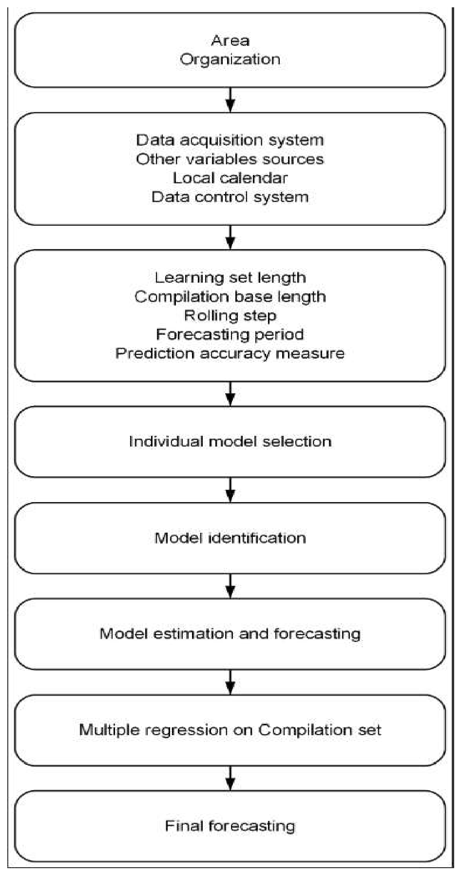
Figure 2.
Electricity load learning set.
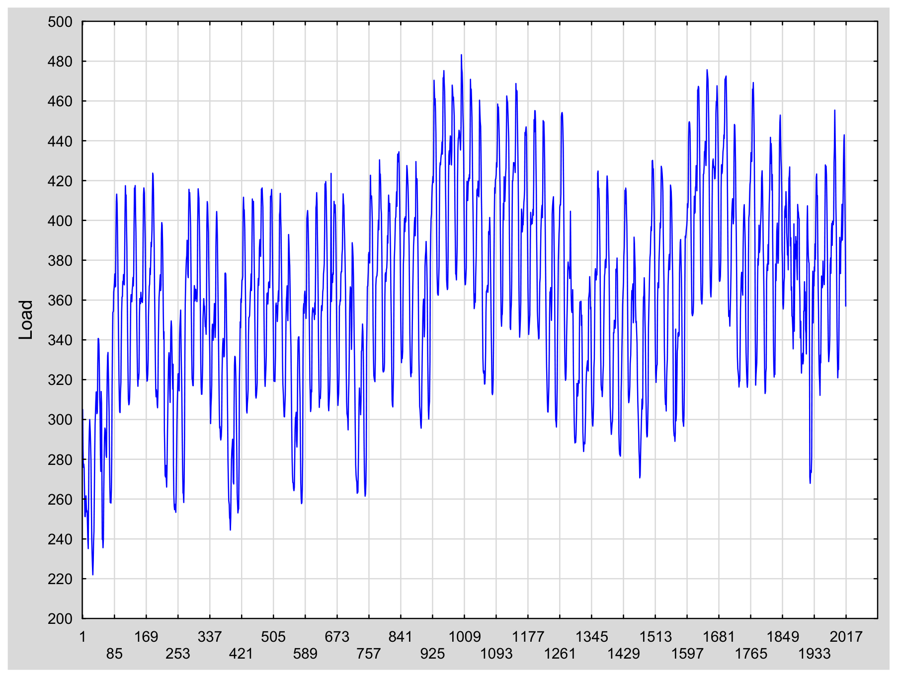
Figure 3.
Average weekly profile of electricity load in learning data.
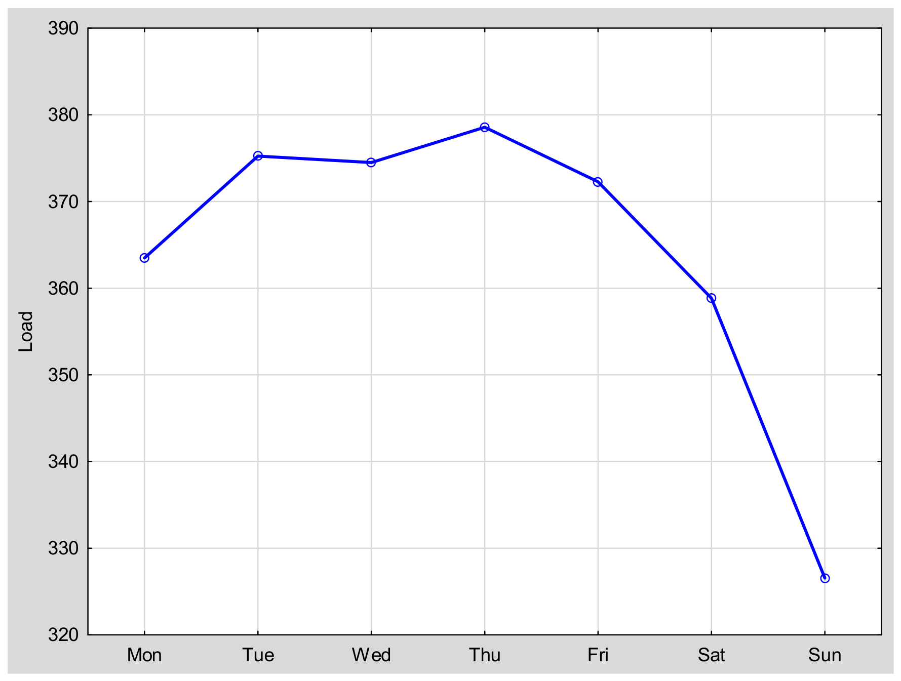
Figure 4.
Average daily profile of learning set electricity load.
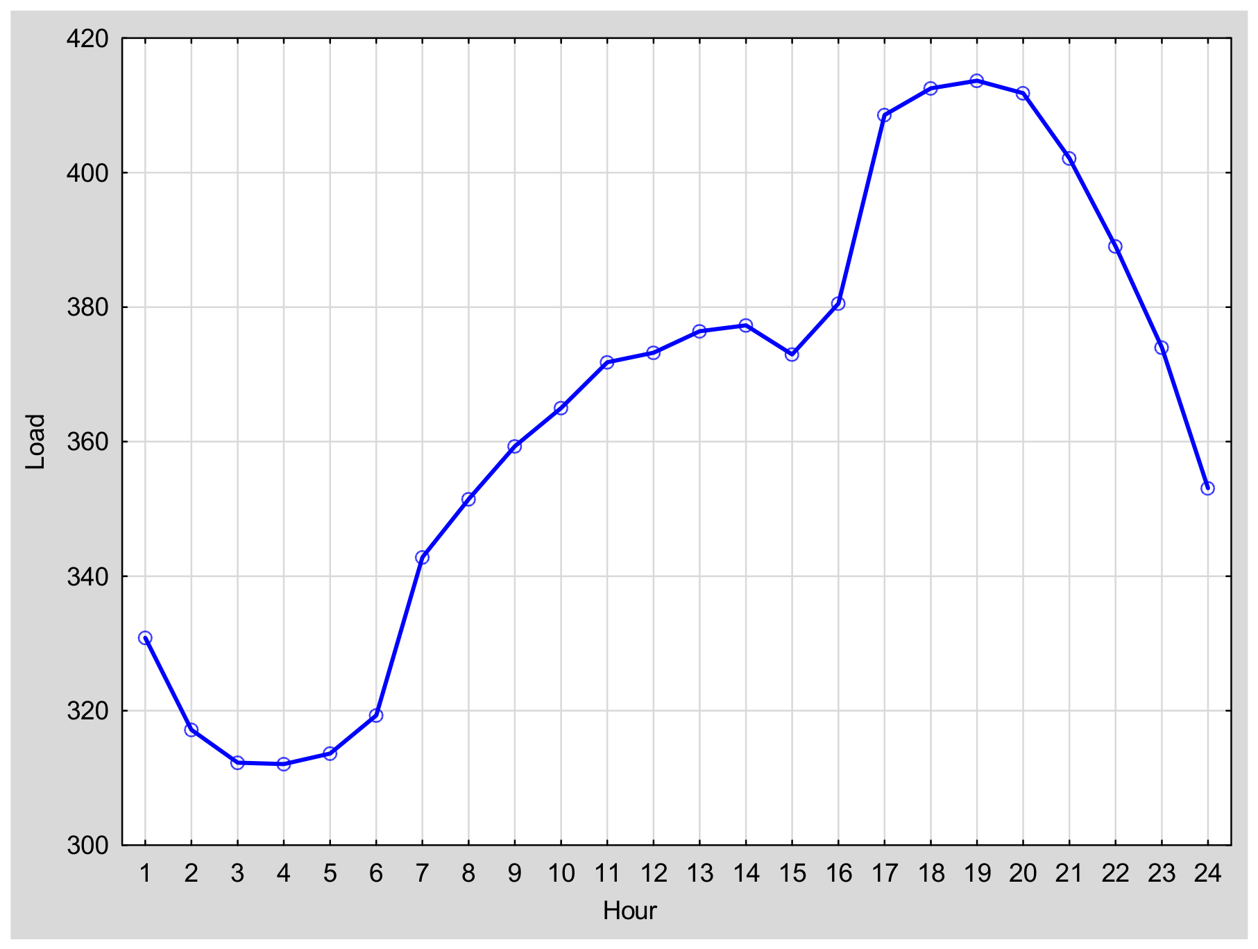

Table 1.
Multiple regression model for electricity load.
| Variable | Coefficient | p-value |
|---|---|---|
| Intercept Average daily temperature t Holiday Monday Tuesday Wednesday Thursday Friday Saturday H1 H2 H4 H5 H6 H7 H8 H9 H10 H11 H12 H13 H14 H15 H16 H17 H18 H19 H20 H21 H22 H23 H24 |
257.617 -2.170 0.016 -62.595 41.864 52.416 55.414 54.883 54.704 32.598 18.611 4.917 -0.209 1.336 6.981 30.470 39.113 46.947 52.637 59.425 60.811 63.989 64.847 60.514 68.071 96.075 100.029 101.153 99.284 89.577 76.481 61.401 40.472 |
0.0000 0.0000 0.0000 0.0000 0.0000 0.0000 0.0000 0.0000 0.0000 0.0000 0.0000 0.1560 0.9518 0.6998 0.0000 0.0000 0.0000 0.0000 0.0000 0.0000 0.0000 0.0000 0.0000 0.0000 0.0000 0.0000 0.0000 0.0000 0.0000 0.0000 0.0000 0.0000 0.0000 |
Source: own calculations
Table 2.
ARIMA model for multivariate regression residuals.
| Parameter | Coefficient | p-value |
| p(1) q(1) Qs(1) |
0.913 -0.065 0.630 |
0.0000 0.0188 0.0000 |
Source: own calculations
Table 3.
ARIMA model for original electricity load time series.
| Parameter | Coefficient | p-value |
|---|---|---|
| p(1) q(1) q(2) q(3) Ps(1) Qs(1) |
0.942 0.959 0.122 -0.100 0.093 0.699 |
0.0000 0.0000 0.0001 0.0001 0.0253 0.0000 |
Source: own calculations
Table 4.
ARIMA model for exponential smoothing residuals.
| Parameter | Coefficient | p-value |
|---|---|---|
| p(1) q(1) q(2) q(3) Ps(1) Qs(1) |
0.946 0.963 0.121 -0.101 0.093 0.699 |
0.0000 0.0000 0.0001 0.0001 0.0246 0.0000 |
Source: own calculations
Table 5.
Multiple regression model combining individual models.
| Variable | Coefficient | p-value |
|---|---|---|
| Intercept Model with dummy variables ARIMA Exponential smoothing Support Vector Regression Artificial Neural Network |
-18.3757 -0.3884 0.5595 0.0599 0.1256 0.7150 |
0.0600 0.0261 0.0000 0.4014 0.4783 0.0020 |
Source: own calculations
Table 6.
Mean Absolute Percentage Errors (MAPE) for individual and final models.
| Model | MAPE for combining period |
MAPE for forecasting period |
|---|---|---|
| Model with dummy variables ARIMA Exponential smoothing Support Vector Regression Artificial Neural Network |
3.26% 2.14% 1.97% 2.49% 2.62% |
4.44% 3.73% 3.91% 4.12% 3.65% |
| Combined Regression model | 0.78% | 3.57% |
Source: own calculations.
Disclaimer/Publisher’s Note: The statements, opinions and data contained in all publications are solely those of the individual author(s) and contributor(s) and not of MDPI and/or the editor(s). MDPI and/or the editor(s) disclaim responsibility for any injury to people or property resulting from any ideas, methods, instructions or products referred to in the content. |
© 2026 by the authors. Licensee MDPI, Basel, Switzerland. This article is an open access article distributed under the terms and conditions of the Creative Commons Attribution (CC BY) license (http://creativecommons.org/licenses/by/4.0/).
Copyright: This open access article is published under a Creative Commons CC BY 4.0 license, which permit the free download, distribution, and reuse, provided that the author and preprint are cited in any reuse.