

Submitted:
24 September 2026
Posted:
28 September 2026
You are already at the latest version
Abstract
Analysing the spatial and temporal variability of near-surface air temperature (Ta) is essential for assessing climate change, particularly in polar regions such as the maritime Antarctic, where observational studies remain comparatively scarce. In areas with sparse meteorological networks, satellite observations provide a valuable means of extending station-based analyses and generating spatially distributed Ta maps. This study analyses updated Ta records from six meteorological stations on the Hurd Peninsula, Livingston Island, for 2000–2024, with particular attention to temperature changes since 2016, and evaluates Ta estimation models based on MODIS Terra daytime LST Collection 6.1 data. The analysis of the Ta time series showed significant warming over the complete 2000–2024 period, with trends ranging from 0.53 to 1.27 °C decade−1, and a clear shift towards warming after 2016. While the 2000–2015 period showed spatially contrasting trends, including cooling at JCI, positive trends were observed at all analysed stations during 2016–2024, ranging from 0.40 to 1.33 °C decade−1 and highlighting substantial local variability across the Hurd Peninsula. The global Ta model, developed using data from all six stations and based on MODIS Terra daytime LST and spatiotemporal variables, achieved a performance comparable to that obtained with Collection 6, with R2 = 0.77 and a cross-validated RMSE of 2.23 °C. The results also showed that rigorous filtering of the MODIS LST observations is essential: retaining only good-quality data and excluding observations with |view angle| > 45° substantially reduced dispersion in the Ta–LST relationship and removed unrealistically low LST values. The introduction of this view-angle threshold represents a new filtering step with respect to our previous studies.
Keywords:
air temperature
; MODIS LST
; temperature trends
; climate warming
; Ta estimation from LST data
; remote sensing
; Hurd Peninsula
; Livingston Island
; South Shetland Islands
; maritime Antarctic
1. Introduction
Antarctica’s maritime sector has experienced temperature changes that challenge our understanding due to its high variability across spatial and temporal scales [1,2].
Turner et al. [3] found that, between 1950 and 2000, the Antarctic Peninsula (AP) experienced a warming that extended, decreasing in intensity, from the southern part of the western AP toward the South Shetland Islands (SSI) and the South Orkney Islands (SOI), with trends ranging from 0.56 °C decade−1 at Faraday/Vernadsky station to 0.20 °C decade−1 at Orcadas station. In contrast, the rest of Antarctica showed air temperature (Ta) trends with much lower and more variable rates, with some stations exhibiting warming and others cooling. The warming on and around the AP since the 1950s had already been noted in previous studies [4,5,6] and was confirmed to have extended until the early 2000s [7], and even up to 2011 at Bellingshausen station (on King George Island, SSI) [8] and Faraday station [9]. The impact of this warming on the cryosphere until 2012 was studied in detail by [10]. Furthermore, studies based on satellite observations using thermal data combined with Ta measurements from automatic weather stations (AWS) between 1957 and 2006 also confirmed warming of the West Antarctic ice shelf [11], particularly concentrated in the AP (≈ 0.38 °C decade−1) [12].
Subsequent studies revealed that Faraday station was an exception, and that most stations experienced cooling during the early part of the 21st century. Turner et al. [13] found an absence of regional warming since the late 1990s when analysing Ta data from six stations located in the northern AP (Rothera, Faraday/Vernadsky, O’Higgins, Esperanza, Marambio, and Bellingshausen). They identified 1998/1999 as the most likely turning point between the warming period (0.32 ± 0.20 °C decade−1, 1979–1997) and the cooling period (–0.47 ± 0.25 °C decade−1, 1999–2014). Oliva et al. [14] analysed interdecadal Ta trends from 1950 to 2015 using data from 10 stations in and around the AP, including the six stations used in [13], as well as San Martín station (on the AP, south of Rothera), Marsh/Eduardo Frei and King Sejong stations (both on King George Island, in the SSI), and Orcadas station (in the SOI). They found that the cooling that began in 1998/1999 was most pronounced in the north and northeast of the AP and the SSI (< -0.5 °C between the decades 1996–2005 and 2006–2015 for the three stations on King George Island), modest in the SOI, and absent in the southwestern AP (Faraday, Rothera, and San Martín stations). Regional modelling and ERA5/ERA-Interim reanalysis-based studies for 1991–2015 have also highlighted the spatial complexity of near-surface Ta changes over the AP, showing contrasting warming and cooling patterns across sectors and seasons (Bozkurt et al. [15]). Recio-Blitz et al. [16] reported a cooling of -0.8 °C over the 12-year period 2004–2016 at Juan Carlos I station (Livingston Island, in the SSI) and assessed its effects on snow density and surface mass balance.
In a later study, Turner et al. [17] extended the analysis of Antarctic temperature variability and change to 17 Antarctic stations, with records updated to 2018. They emphasized the strong spatial variability of near-surface Ta trends across Antarctica and the important role of winter temperature variability, atmospheric circulation, sea-ice conditions and tropical Pacific forcing. For the northern AP, they reported that the warming from the late 1970s to the late 1990s was followed by a small cooling during the 2000s, associated with enhanced easterly flow and increased sea ice near the tip of the Peninsula. However, they also noted an upturn in the Northern Peninsula stacked annual temperature record, with positive anomalies since 2016, linked to negative sea-ice concentration anomalies around Esperanza and Marambio and, in 2017–2018, also off Vernadsky and Rothera. Since the end of the period analysed by Turner et al. [17], several studies and climate assessments have reported renewed warm conditions and extreme events over the AP. For instance, Carrasco et al. [18] revisited observed near-surface Ta variability across eight stations in the AP region over 1978–2020 and suggested that the mid-2010s may mark the end of the early-21st-century warming pause. In February 2020, Esperanza station recorded 18.3 °C, the World Meteorological Organization (WMO)-recognized record high temperature for the Antarctic continent. In February 2022, the AP experienced another extreme warm event and record-high surface melt, comparable to the warm episodes of 2015 and 2020 (Gorodetskaya et al. [19]). Consistently, the 2022 Antarctic climate assessment reported that 2022 was the second-warmest year on record at the five long-term staffed weather stations located on the AP, with three of them recording their warmest July–December period (Clem et al. [20]). On Livingston Island, Recio-Blitz et al. [21] analysed the climatic mass balance of Hurd and Johnsons glaciers over 2002–2016, documenting the glacier response to the transient cooling period in the northern AP and SSI. They placed this period in the context of the subsequent return to warming conditions reported for the region by Carrasco et al. [18]. More recently, studies based on Spanish meteorological observations and PERMATHERMAL Ta records have improved the local climatological characterisation of Livingston and Deception islands, extending the observational context into the 2020s (González-Herrero et al. [22]; de Pablo and Goyanes [23]). González-Herrero et al. [22] also emphasized that the western sector of the SSI, including Livingston Island, has received less scientific attention than King George Island. In addition, Luengo- S et al. [24], in a study mainly focused on seawater temperature records at Livingston and Deception islands, analysed nearby AEMET Ta series and reported positive Ta changes over the 10-year period 2015–2025, equivalent to approximately 1.18 °C decade-1 at JCI and 0.77 °C decade-1 at Gabriel de Castilla.
Recondo et al. [1] studied daily mean Ta data from six Spanish stations on the Hurd Peninsula, Livingston Island (SSI), from 2000 to February 2016. The meteorological stations included three managed by the Spanish State Meteorological Agency (AEMET): Juan Carlos I (JCI), Johnsons Glacier (JG), and Hurd Glacier (HG), and three stations from the PERMATHERMAL network operated by the University of Alcalá [25,26]: Incinerador (INC), Reina Sofía (SOF), and Collado Ramos (CR). The analysis of the Ta time series revealed differences among locations: the station closest to the coast (JCI) showed a cooling trend, while the higher-altitude stations showed warming trends (between 0.3 and 0.9 °C decade−1), highlighting the complex spatial climatic variability on the Hurd Peninsula.
To further investigate this spatial variability and expand upon our previous work [1], the present study analyses updated Ta time series from 2000 to early 2024. Particular attention is given to the period since 2016, for which, to our knowledge, local Ta trends on Hurd Peninsula have not yet been specifically assessed. This extended dataset enables us to examine whether the trends identified in the 2000–2015 period have persisted, intensified, or changed sign, providing new insights into recent temperature evolution in this sector of the maritime Antarctic.
In addition, satellite observations offer an additional means of extending station-based analyses to areas where in situ meteorological observations are sparse or unavailable, although the availability of thermal satellite data in polar regions is strongly limited by frequent cloud cover, which reduces the number of valid land surface temperature (LST) observations. Although near-surface Ta is not directly measured by satellite sensors, previous studies have shown that it can be estimated from satellite-derived LST and ancillary variables [27] and references therein, [28], with applications in different regions worldwide. Among thermal satellite products, LST data from the Moderate Resolution Imaging Spectroradiometer (MODIS), on board NASA’s Terra and Aqua satellites [29], have been widely used for this purpose.
In polar regions, however, studies comparing near-surface Ta with satellite-derived LST remain relatively limited. Most previous work using MODIS LST data has focused on Arctic or sub-Arctic environments, including Greenland and pan-Arctic analyses, where the strength of the Ta–LST relationship has been shown to vary according to surface conditions, season, temperature range, and cloud-screening performance. Nevertheless, these studies generally reported positive Ta–LST relationships, with R2 values often above 0.6 [30,31,32,33,34].
In Antarctica, Wang et al. [35] compared monthly MODIS LST Collection 5 (C5) with in situ Ta from eight automatic weather stations in the Lambert Glacier Basin, East Antarctica, and reported statistically significant relationships, although with spatial differences among stations. Meyer et al. [36] estimated Ta across the Antarctic continent from MODIS LST C5 and auxiliary variables using both linear regression and machine-learning approaches, showing that MODIS LST can support continental-scale Ta estimation. More recently, Antarctic-scale studies have further used MODIS-derived surface temperature information to reconstruct or assess near-surface air temperature. Zhang et al. [37] reconstructed monthly near-surface Ta over the Antarctic Ice Sheet from MODIS LST and in situ observations. Nielsen et al. [38] developed AntAir ICE, a daily 1 km2 near-surface Ta dataset for Antarctica and its ice shelves derived from MODIS land and ice surface temperature. Xie et al. [39] reconstructed Antarctic surface air temperature (SAT) from MODIS LST using ERA5-derived LST–SAT relationships and in situ bias correction, reporting a warming tendency in the AP over 2001–2023, although regional trends were not statistically significant when data and fitting uncertainties were considered. However, these Antarctic-scale studies were not focused on local Ta modelling in the AP or the maritime Antarctic.
In terms of satellite-based Ta estimation in the AP region, our previous work [1] was, to our knowledge, the first study to develop empirical models for estimating Ta from MODIS LST, specifically on Hurd Peninsula, Livingston Island. That study used daily mean Ta from the same six AEMET/PERMATHERMAL meteorological stations considered here, together with MODIS LST C5 data and spatiotemporal variables. Multiple linear regression (MLR) models were tested using Terra and Aqua MODIS LST, both daytime and nighttime, for the period 2000–2016. The best global Ta model was obtained with Terra daytime LST data, with R2 = 0.6 in the model generation and RMSECV = 2.6 °C in the validation. A second previous study (Corbea-Pérez et al. [2]) used the same Ta dataset and study period, but with MODIS LST Collection 6 (C6) data instead of C5. This resulted in a significant improvement over C5, with the Terra daytime global model reaching R2 = 0.8 and RMSECV = 2.2 °C. Together, these studies confirmed the potential of MODIS LST for estimating daily mean Ta in this sector of the maritime Antarctic.
The second objective of the present study is therefore to use MODIS Terra daytime LST C6.1 data (an updated version of C6) and to extend the development and evaluation of Ta estimation algorithms to the period 2000–2024, using an expanded observational dataset, in order to produce improved spatially distributed Ta maps for Livingston Island.
2. Materials and Methods
2.1. Study Area
The study area is the Hurd Peninsula of Livingston Island, in the South Shetland Islands (SSI), Maritime Antarctica, off the north-western Antarctic Peninsula (Figure 1). This archipelago extends between approximately 61°55′S–63°30′S and 57°45′W–61°30′W, about 100 km from the Antarctic Peninsula (AP) and around 1000 km from Tierra del Fuego. It includes several islands, among them King George, Livingston and Deception Islands, and is separated from the AP by the Bransfield Strait and from South America by the Drake Passage. The region has a maritime Antarctic climate, with a mean annual Ta of about −2 °C [40], summer mean Ta values that may rise to around 2 °C [41], annual precipitation of about 500−800 mm [41], and extensive snow and ice cover.
Livingston Island is the second largest island of the SSI, with an area of approximately 974 km2, a length of about 73 km, and a variable width between 5 and 34 km [41]. Around 90% of its surface is permanently ice-covered, while only the western sector and some coastal areas become snow-free during summer [41]. These summer snow-free areas include Byers Peninsula, on the western side of the island, and Hurd and Rozhen Peninsulas, in the south [41]. Hurd Peninsula is located between South Bay and False Bay (Figure 1). This peninsula hosts the Spanish Antarctic Station (SAS) Juan Carlos I, which has been operating since January 1988, about 50 m from the western coast of the peninsula and at an elevation of 12 m above sea level (a.s.l.). Behind the station, the terrain rises towards a mountainous barrier that almost reaches 300 m near the station and continues inland towards the Friesland Mountains, about 10 km away [41]. The peninsula also includes several meteorological and permafrost monitoring sites distributed across coastal, glacierized and higher-elevation settings, including the six stations analysed in this study (Figure 1). Detailed information on the AEMET meteorological stations in the South Shetland Islands can be found in Bañón and Vasallo [41], while a concise meteorological summary of the AEMET stations located on Hurd Peninsula is provided in Recondo et al. [1].
2.2. In Situ Ta Data from Meteorological Stations
The Ta data (~2 m above ground) used in this study were obtained from AEMET stations (JCI, JG, and HG) and from three PERMATHERMAL network sites (INC, SOF and CR) on Hurd Peninsula (Figure 1). The study period extends from 1 January 2000 to 23 March 2024, with the initial year determined by the availability of MODIS LST data, and the end date by the last AEMET data collected during the 2023/2024 Antarctic summer campaign. The data from 2000 to 2015 were compiled and analysed in our earlier study [1], while the data from 2016 to 23 March 2024 have been compiled for the present work. The more recent JCI data (2016–2024) were retrieved from the AEMET Open Data Application Programming Interface (API): https://opendata.aemet.es/centrodedescargas/inicio. In both studies, we used only daily mean Ta, calculated at each station only when the intraday measurements (recorded at 10- or 30-minute intervals) were complete. All data (2000–2024) are jointly analysed in Section 3.1.
The JCI station began operating on 16 February 1988 and was relocated approximately 100 m westward to its current position (Table 1) on 31 December 2009. This change in location, along with changes or possible failures in the early instrumentation, led to inconsistencies in Ta values. Consequently, the data from the initial location (1 January 2000 to 30 December 2009) were empirically corrected and homogenized in Recondo et al. [1]. The JG station started recording data on 1 December 2006 and was relocated from Johnsons Glacier to Hurd Glacier on 25 January 2015 and has since been known as the HG station (Table 1). These are considered separate stations due to the considerable distance between their locations (Figure 1). The instrumentation used at each AEMET station over time is described in detail in [1]. The height of the AEMET Ta sensors is 1.8 m above ground, and the instrumental accuracy of temperature measurements at the three stations is ±0.1 °C [1].
The PERMATHERMAL stations operated by the University of Alcalá (UAH) were originally installed by Miguel Ramos and his team, and are currently maintained by Miguel de Pablo and his group. The INC station was installed on 25 February 2000 in the same meteorological shelter as the JCI AEMET station, where it remained until 2005. In January 2006, the station was moved to its current location (Table 2), approximately 300 m from the original site, and the Ta sensor height was adjusted from 3.0 m to 1.60 m. Due to problems with the initial sensors (2000–2001), the Ta measurements from that period were discarded. In 2002, the sensors were upgraded, with an estimated error between ±0.3 °C and ±0.4 °C. Nevertheless, only the INC data from its current location (from 2006 onward), independent of JCI, have been used in this study. These data were also empirically corrected and homogenized in Recondo et al. [1]. The SOF station was installed on 25 February 2000 at the summit of Mount Reina Sofía (Table 2), using instrumentation similar to that at INC during the same period; therefore, its data prior to 2002 were also discarded. The CR station was installed on 2 February 2006 at the summit of an unnamed hill (Table 2), using sensors similar to those used at INC since 2005. Both SOF and CR stations have experienced data gaps during the study period due to various instrumentation problems. The Ta sensors are positioned 1.05 m and 1.60 m above ground, respectively. The instrumentation used at each PERMATHERMAL-UAH station over time is described in detail in [1].
2.3. MODIS Data
We used the MODIS Collection 6.1 (C6.1) Land Surface Temperature and Emissivity (LST/E) Daily L3 Global 1 km Grid Sinusoidal (SIN) product (MOD11A1.061 for the Terra satellite; MOD refers to a MODIS/Terra product, and 061 refers to C6.1), which is provided by the NASA Land Processes Distributed Active Archive Center (LP DAAC) [42]. In addition, for further filtering of the LST data, we also used the MODIS C6.1 Snow Cover Daily L3 Global 500 m Grid (SIN) product (MOD10A1.061), which is provided by the NASA National Snow and Ice Data Center (NSIDC) Distributed Active Archive Center [43]. Data from these products were obtained through the Google Earth Engine (GEE) [44] (http://earthengine.google.org) API (https://code.earthengine.google.com/).
The theoretical basis of the 1 km MODIS LST/E products was established by Wan and Dozier [45], while the C6.1 documentation and user guide, and the C6 validation, are provided in several documents and articles by Wan [46,47,48]. These products are filtered using cloud and land/water masks (1-km resolution), so that LST/E data are provided only under clear-sky conditions and over land (including snow-covered land, but not ice) or inland water [47]. They also include a quality control (QC) assessment. The 500 m MODIS Snow Cover products contain snow cover, snow albedo, fractional snow cover, and quality assessment (QA) data [49]. These products also include a classification of the type of cover: snow, land (no snow), water (ocean or inland water (lake)), and cloud. This classification (at 500 m resolution) has been used in our studies to try to improve the LST filters.
The MODIS LST/E C6 product improved the LST data obtained from C5, mainly due to the improvement of the cloud filters and the emissivity values for bands 31 and 32, and to a modification of the Generalized Split-Window (GSW) algorithm used in C5. Details can be found in the works by Wan [47,48] and a brief summary is provided in Corbea-Pérez et al. [2]. Wan’s comparisons between LST data (C5 and C6) and in situ surface temperatures (Ts) showed that the accuracy of these LSTs is better than 1 °C in most of the study sites (all clear-sky cases) [48]. At the South Pole site included in the C6 validation, the error obtained was -0.5 °C [48]. The scientific algorithm of the MOD11 product in C6.1 is unchanged with respect to C6; differences between C6 and C6.1 are mainly related to improvements in the calibration of the input MODIS L1B products and polarization corrections [47].
The MODIS LST data were filtered following the procedure described in Recondo et al. [1] (their Appendix C), using the quality-control (QC) codes expressed as binary numbers, as explained by Wan [47]. These QC codes are provided as integer values in C6.1, but their binary representation was used to identify the corresponding bit-level quality flags. A major difference between C6.1 and the C5 product used in [1] was observed in the number of QC values. Whereas up to seven different QC values were found in the MODIS C5 data extracted at the locations of the studied meteorological stations, only five QC values were found in the C6.1 data for the same stations: 2 (no LST data), 0, 8, 65 and 73, of which only three (2, 0 and 65) were also present in C5. The MODIS product itself discarded a large number of observations due to cloud effects (QC = 2), leaving simultaneous Ta–LST data available for only about 33–38% of the total records at JCI, INC, SOF and JG, 29% at CR and 17% at HG. Among the remaining observations, good-quality observations (QC = 0 and QC = 8) represented only about 2–8% of the available Ta–LST data, whereas QC = 65 accounted for 83–97% and QC = 73 for 2-9% (Table 3 and Figure 2). Figure 2 illustrates, using JCI as an example, the MODIS filtering procedure. QC = 65 and QC = 73 observations show a large dispersion and extremely low LST values compared with the corresponding Ta values, resulting in a very weak linear relationship between Ta and LST (R2 = 0.12; Figure 2a). Some outliers nevertheless remained and were mainly associated with high sensor view angles (>45°), which tended to underestimate LST. In our data, this effect became evident beyond approximately 45°, consistent with the 45° limit commonly adopted in LST retrieval algorithms [47], although MOD11 does not apply this angular threshold. Observations with |view angle| > 45° were therefore removed, increasing R2 to 0.78 (Figure 2c). A similar improvement was observed at the other stations, except HG, where the number of good-quality observations was small and no cases exceeded this threshold. The application of this angular threshold to good-quality observations represents an improvement in the filtering procedure compared with our previous studies. In [1], no additional angular filtering was applied to good-quality observations, whereas in [2] outliers were removed based on a statistical criterion. This angular threshold was also evaluated as a possible way to retain part of the QC = 65 observations, since these represented the majority of the available data. Although applying the threshold removed many observations with anomalously low LST, a substantial number of such values remained and continued to produce considerable dispersion. A similar, and even more pronounced, behaviour was observed for QC = 73, which was therefore discarded entirely. For QC = 65, the effects of clear-sky coverage and satellite overpass time were also examined, but neither criterion successfully removed the anomalous observations. In the case of overpass time, however, the available range was relatively narrow (approximately 07:00–11:00 local solar time).
| QC_int | QC_binary | Descripción |
| 2 | 00000010 | 10 = LST not produced due to cloud effects; 00 = good data quality; 00 = average emissivity error ≤ 0.01; 00 = average LST error ≤ 1K |
| 0 | 00000000 | 00 = LST produced, good quality, not necessary to examine more detailed QA; 00 = good data quality; 00 = average emissivity error ≤ 0.01; 00 = average LST error ≤ 1K |
| 8 | 00001000 | 00 = LST produced, good quality; 10 = TBD; 00 = average emissivity error ≤ 0.01; 00 = average LST error ≤ 1K |
| 65 | 01000001 | 01 = LST produced, other quality, recommend examination of more detailed QA; 00 = good data quality; 00 = average emissivity error ≤ 0.01; 01 = average LST error ≤ 2K |
| 73 | 01001001 | 01 = LST produced, other quality, recommend examination of more detailed QA; 10 = TBD; 00 = average emissivity error ≤ 0.01; 01 = average LST error ≤ 2K |
Regarding the filters based on the MOD10A1 product, the “NDSI_Snow_Cover_Algorithm_Flags_QA” layer was also examined to identify possible residual cloud contamination. In particular, observations flagged as “probably cloudy” (bit 5) were analysed. These occurred in 1 case at JCI, 1 at JG, none at HG, 3 at INC, 22 at SOF, and 8 at CR. Their removal did not improve the Ta –LST relationship at most stations and produced only a marginal improvement at SOF, where they were most frequent. Therefore, these observations were retained.
The MODIS data used in this study cover the period from 5 March 2000 to 23 March 2024 (24 years). The initial date was determined by the availability of Terra-MODIS LST data, whereas the final date corresponds to the last Ta AEMET data available for this work, collected during the 2023/2024 Antarctic summer campaign. In this study, we used only daytime Terra-MODIS LST data, because they gave the best results in our previous works [1,2].
2.4. Other Data
The relationship between near-surface Ta and satellite-derived LST is known to be affected by environmental and spatio-temporal factors, especially in topographically complex regions [1,50]. Therefore, additional variables related to topography, location, and time, including seasonality and the Terra-MODIS overpass time, were also considered in this study.
The topographic variables included in the model to estimate Ta were obtained from the Advanced Land Observing Satellite (ALOS) World 3D digital elevation model (AW3D), released by the Japan Aerospace Exploration Agency (JAXA) in 2016 [51]. AW3D was generated using images from the Panchromatic Remote-sensing Instrument for Stereo Mapping (PRISM) sensor, onboard ALOS. The dataset used in this study has a spatial resolution of 30 m (AW3D30) [51] and was selected after visual inspection of available DEMs over the study area, because it provided a consistent elevation surface and ensured methodological consistency with our previous studies [1,2]. The raster variables derived from the digital elevation model (DEM), in addition to height (in m) for each pixel, were: slope (dimensionless), roughness (dimensionless), curvature (m-1), and orientation (radians, dimensionless) (Table 4). Slope, roughness, and orientation were derived following the formulas described by Felicísimo [52], with slope computed using an eight-neighbour filter and roughness calculated as the variance of slope. Curvature was computed using an eight-neighbour Laplacian filter with a positive central coefficient (+8) and negative coefficients for the surrounding neighbours (−1), so that ridges have positive curvature and valleys have negative curvature. The topographic variables were calculated using ESA’s SNAP software, except orientation, which was derived using ArcGIS.
Latitude and longitude (in degrees) and distance to the coast (in m) (Table 4) were used as location variables, the latter to account for the degree of continentality or maritime influence of each pixel. Time (expressed as decimal year), its first harmonic terms (sine and cosine), and the local solar time of the daytime Terra-MODIS overpass (in hours) were used as temporal variables.
2.5. Methodology
For the analysis of the Ta time series, following Recondo et al. [1], the temporal variability of Ta at each station was analysed by fitting Ta as a function of time, Ta =f (t), where (t) is expressed in decimal years. The model includes a linear time term to represent the warming or cooling trend and one sine–cosine harmonic pair to account for the annual seasonal variation in Ta:
where (ci) are the regression coefficients. The inclusion of additional harmonics, such as sin 4t/cos4 was not necessary because the first harmonic adequately represented the seasonal cycle. All variables retained in the model were statistically significant (p < 0.05).
A multiple linear regression (MLR) model was used to estimate Ta from the combined dataset of all stations included in the study, following Recondo et al. [1]. The global Ta model included LST, the three temporal variables used in the linear-harmonic model (Equation 1), and the nine additional predictor variables described in Section 2.4, giving a total of 13 predictor variables. The general structure of the model was:
where is the intercept, – are the regression coefficients, and LST are expressed in °C, is time expressed in decimal years, and represents the nine additional predictor variables described in Section 2.4. Only statistically significant predictors (p < 0.05) were retained in the final model.
The statistical analyses and graphical outputs were performed using the free R software environment (http://www.r-project.org/) [53]. In all cases, robust regression models, which are less sensitive to outliers than ordinary least-squares regression, were fitted using the MASS package in R [54]. The statistics used to assess model goodness of fit were the coefficient of determination (R2), and the residual standard error (RSE): , whereis the value of y predicted by the model and ν denotes the residual degrees of freedom, calculated as the number of observations, , minus the number of estimated model parameters, (e.g., ν = n – 2 in a simple linear regression). Because of the limited number of observations, all available data were used to fit the model.
Model performance was evaluated using leave-one-out cross-validation (CV). The validation statistics were the cross-validated coefficient of determination (R2CV), the cross-validated root mean square error (RMSECV): , where yobserved is the observed data and yestimated the data estimated by model; the MAE: , the ratio of performance to deviation (RPD): , where σ is the standard deviation of the reference data, and the bias for the mean of the residuals:
3. Results
3.1. Analysis of the Ta Time Series
The daily mean Ta series at the stations show a sinusoidal behavior with a linear trend over the full study period (2000-2024) (Figure 3 and Figure 4; Table 5), as well as over the partial periods 2000–2015 and 2016–2024 (Table 5), according to Equation (1). In only two cases, no trend over time was detected (slope=0), as the time variable (t) was not statistically significant (p > 0.05): JG for its complete record (2006–2015, which is the same dataset included in the 2000–2015 analysis) and INC during 2000-2015. In the case of JG, the absence of a trend may be attributed to limited data availability. For HG, despite data gaps, a linear trend could be determined for its full available record within 2000–2024 (t was significant, p ≈ 0.02), and also for 2016-2024 (t was significant, p ≈ 0.001). However, during 2000–2015, the scarcity of data prevented a reliable fit (R2 = 0.27). The linear trend was also significant for CR over 2000–2024 (p ≈ 0.001) and for SOF over 2016–2024 (p ≈ 0.01). In the remaining series, the linear trends are clearly defined, with t and the other predictors being highly significant (in most cases with p < 2 × 10⁻¹⁶).
For the complete 2000–2024 study period, Table 6 shows warming trends at all stations except JG. This overall warming pattern is also visually apparent in Figure 3 and Figure 4. In general, the magnitude of the trend, expressed by the slope (α), increases from the lower- to the higher-elevation stations. HG (h = 93 m) is the only station that does not strictly follow this pattern, as its slope is slightly lower than that of INC (h = 34 m), 0.07 and 0.08 °C year−1, respectively. However, it should be noted that the HG record only covers the period 2015–2022. To show the relationship between elevation and warming more clearly, the stations were ordered by elevation in Table 6, and the slopes were expressed in °C decade−1, as is customary in the literature. The warming trend increases from 0.53 °C decade−1 at the lowest-elevation station, JCI, to 1.27 °C decade−1 at the highest-elevation station, SOF, with intermediate values of 0.78 °C decade−1 at INC, 0.67 °C decade−1 at HG, and 1.13 °C decade−1 at CR.
To assess whether warming intensified during 2016–2024 relative to the preceding 2000–2015 period, trends were calculated separately for both sub-periods at all stations for which sufficient data were available. The full results are presented in Table 5, while Table 6 provides a summary together with the trends for the complete 2000–2024 period.
During the recent 2016–2024 period, all stations showed positive temperature trends, although the magnitude of warming did not increase systematically with elevation. The highest trends were observed at INC, HG and CR, with values between 1.25 and 1.33 °C decade−1 (for CR and INC, respectively), whereas the lowest trend occurred at SOF, the highest-elevation station, with 0.40 °C decade−1. Comparison with the preceding 2000–2015 period shows a reversal from cooling to warming at JCI, the emergence of a significant warming trend at INC, and a marked increase in the warming rate at CR. In contrast, the warming trend at SOF was weaker during the recent period. A direct comparison could not be made for HG because of insufficient data during 2000–2015.
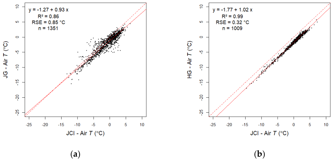
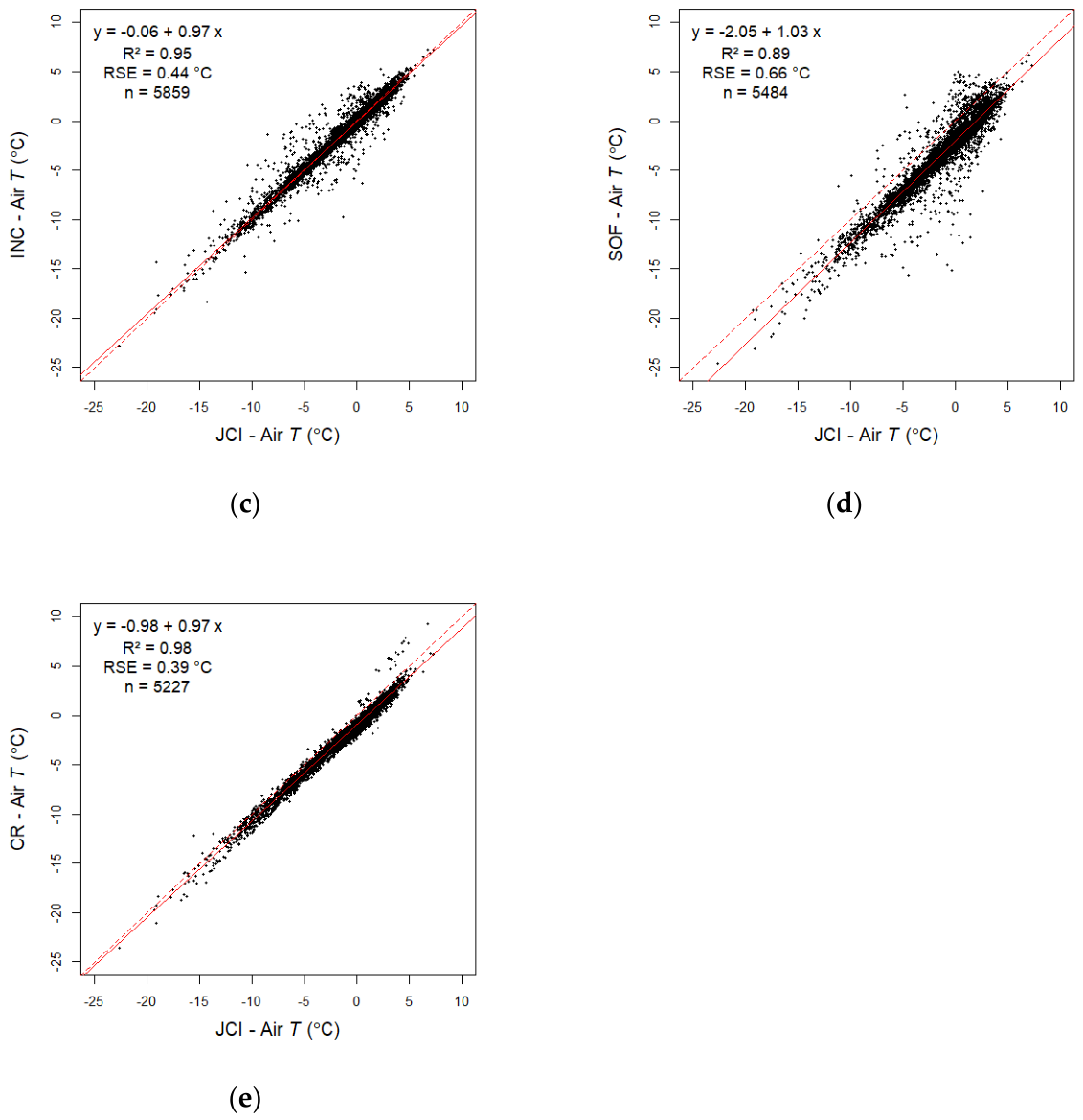
Finally, Appendix A presents the linear relationships between Ta at each station and Ta at the AEMET reference station, JCI (Figure A1). Although this is not the main objective of the study, these relationships could be useful for filling data gaps in some of the station records.
3.2. Global Ta Model Based on MODIS LST and Spatiotemporal Variables
The results obtained with the global MLR model (Equation (2)), based on Terra daytime LST and the combined dataset from all six stations, are shown in Table 7. The model yielded R2 = 0.77 and RSE = 1.52 °C. The statistically significant predictors (p < 0.05) retained in the final model were LST, linear time (t), the sine-cosine pair of the annual harmonic, the local solar time of the LST observation (H), longitude (l), roughness (r), and curvature (c). The complete sine–cosine pair was retained when the annual harmonic was jointly significant, even if one of its components was not individually significant.
3.3. Validation of the Ta Estimation Model
The leave-one-out cross-validation results for the global Terra-Day model are shown in Table 8. The R2CV obtained in the validation was only slightly lower than the R2 obtained during model fitting, whereas the RMSECV was greater than the RSE obtained during model fitting. The model yielded R2CV = 0.75, RMSECV = 2.23 °C, MAE = 1.51 °C, RPD = 2.00, and a bias of 0.05 °C.
4. Discussion
The results obtained for Hurd Peninsula indicate a clear change in Ta evolution since 2016. Over the complete study period (2000–2024), all stations with sufficiently long records (JCI, INC, HG, CR, and SOF) showed significant warming trends, ranging from 0.53 °C decade−1 at the coastal JCI station to 1.27 °C decade−1 at SOF, the highest-elevation station. However, the comparison between the two sub-periods provides a more informative picture. During 2000–2015, JCI cooled at −0.38 °C decade−1, INC showed no significant trend, and CR and SOF warmed at 0.39 and 0.87 °C decade−1, respectively. By contrast, all five stations showed positive trends during the recent 2016–2024 period, with warming rates of 0.78 °C decade−1 at JCI, 1.33 °C decade−1 at INC, 1.30 °C decade−1 at HG, 1.25 °C decade−1 at CR, and 0.40 °C decade−1 at SOF. Thus, the clearest evidence of a recent change is found at JCI, where the sign of the trend reversed, and at INC and CR, where warming either emerged or became markedly stronger.
The recent warming observed since 2016 is consistent with the broader Ta evolution reported for the northern AP. Turner et al. [17] identified an upturn in the Northern AP Ta record, with positive anomalies from 2016 onward, after the small cooling observed during the 2000s. Similarly, Carrasco et al. [18] suggested that the mid-2010s may have marked the end of the early-21st-century warming pause. Our results provide local observational evidence that this regional change also occurred on Hurd Peninsula: the 2016–2024 trends were positive at all five stations analysed and exceeded 1.2 °C decade−1 at INC, HG, and CR. The results therefore support the interpretation that the cooling or reduced warming observed during the first part of the century was followed by renewed warming, although the magnitude of this change varied considerably among sites.
At JCI, the cooling trend obtained for 2000–2015 (−0.38 °C decade−1), corresponding to a total linear decrease of approximately -0.61 °C over this 16-year period, is consistent in sign and magnitude with the cooling of -0.8 °C reported by Recio-Blitz et al. [16] for 2004–2016 (a 12-year period). The values are not identical because the study periods and analytical procedures differ, but both analyses independently identify cooling at JCI before 2016. In the present study, however, this cooling was followed by a warming trend of 0.78 °C decade−1 during 2016–2024, corresponding to an estimated increase of approximately 0.64 °C over the available 8.2-year period.
The recent JCI trend is also consistent with the positive Ta change reported by Luengo-S et al. [24], who obtained an increase of 1.18 °C over the approximately 10-year period 2015–2025. Their value is somewhat larger than the increase of 0.64 °C estimated here for 2016–March 2024, but both studies clearly identify renewed warming at JCI. The difference may partly reflect the different study periods, data aggregation, and trend-estimation methods used in the two studies; Luengo-S et al. analysed Ta data sampled at 20 min intervals, whereas the present study used daily mean Ta calculated only from complete daily records.
For the complete records, the warming rate generally increased with elevation, from 0.53 °C decade−1 at JCI to 1.27 °C decade−1 at SOF. Nevertheless, this apparent elevation dependence should be interpreted cautiously. It is based on a small number of stations with unequal record lengths, and it was not maintained during 2016–2024: SOF, at 271 m a.s.l., showed the lowest recent trend (0.40 °C decade−1), whereas the largest trends occurred at the lower-elevation INC, HG, and CR stations. Therefore, elevation alone cannot explain the spatial differences in recent warming. Local exposure, distance from the coast, surface conditions, snow cover, and differences in data availability may also contribute to the observed between-station variability.
These results reinforce the value of maintaining long-term meteorological observations on Hurd Peninsula, where stations located within less than 4 km of each other show different warming rates.
With regard to the second objective of the study, the global Terra-Day model developed using MODIS LST C6.1 and the combined dataset from the six stations yielded R2 = 0.77 and an RSE of 1.52 °C. Leave-one-out cross-validation produced R2CV = 0.75, RMSECV = 2.23 °C, MAE = 1.51 °C, an RPD of 2.00, and a bias of 0.05 °C. These results are similar to those reported by Corbea-Pérez et al. [2] for the global C6 Terra-Day model for Livingston Island, which yielded R2=0.76 and RSE=1.56 °C during model fitting, and R2CV = 0.75, RMSECV = 2.19 °C, MAE = 1.60 °C, and a bias of 0.01 °C in the validation. Extending the study period to 2024 and increasing the number of observations from 368 to 568 did not produce substantial changes in model goodness of fit or validation errors. This correspondence indicates that the model retains a similar statistical performance to that obtained with C6 for the 2000–2016 period. Although both models retained eight predictors, the present model retained the complete sine–cosine pair, included longitude, and used a revised curvature calculation based on an eight-neighbour filter (rather than the four-neighbour filter used in the previous model). However, the present model achieved comparable performance with fewer topographic predictors (only curvature and roughness) than the previous C6 model, which retained four topographic predictors (slope, elevation, roughness, and orientation, but not curvature). This reduced dependence on topographic predictors may be related to the improved curvature calculation, but also to the angular filtering introduced in the present study, which may select more reliable LST observations than the auxiliary statistical filtering used previously.
5. Conclusions
The updated Ta series indicate that Hurd Peninsula experienced renewed warming from 2016 onward. Over the complete 2000–2024 period, all stations with sufficiently long records showed significant warming trends, whereas the comparison between 2000–2015 and 2016–2024 revealed a clear shift towards positive trends at all analysed stations. This change was especially evident at JCI, where the trend shifted from cooling to warming, and at INC and CR, where warming emerged or intensified during the recent period. The results support the view that the early-21st-century warming pause in the northern AP ended around 2016, while also showing that recent warming was spatially heterogeneous on Hurd Peninsula. The different warming rates observed among nearby stations suggest that local factors may modulate the regional climate signal, highlighting the importance of maintaining long-term meteorological observations on Livingston Island and, more broadly, across the South Shetland Islands.
The global model based on MODIS Terra-Day C6.1 maintained a performance comparable to that previously obtained with C6, despite the extension of the study period and the increase in the number of observations. Applying a filtering criterion based on the sensor view angle substantially reduced the occurrence of anomalously low LST values and the dispersion in the Ta–LST relationship. These results support the combined use of meteorological observations and MODIS data to analyse air temperature on Hurd Peninsula, although cloud cover continues to limit the availability of valid satellite observations.
Author Contributions
Conceptualization, C.R.; methodology, C.R., A.C.-P. and M.R.G.-M.; software, C.R., A.C.-P. and E.P.-R.; validation, C.R. and A.C.-P.; formal analysis, C.R., A.C.-P. and E.P.-R.; investigation, C.R., A.C.-P., M.R.G.-M. and E.P.-R.; resources, C.R., A.C.-P., M.R.G.-M., E.P.-R., M.A.dP. and C.A.-P.; data curation, C.R., A.C.-P., E.P.-R. and M.A.dP.; writing—original draft preparation, C.R.; writing—review and editing, C.R., A.C.-P., M.R.G.-M., E.P.-R., M.A.dP. and C.A.-P.; visualization, C.R., A.C.-P. and E.P.-R.; supervision, C.R.; project administration, C.R.; funding acquisition, C.R. All authors have read and agreed to the published version of the manuscript.
Funding
This research received no external funding.
Data Availability Statement
MODIS data used in this study are publicly available from NASA repositories and through Google Earth Engine. AEMET meteorological data are available through AEMET OpenData. The remaining meteorological data and the processed datasets generated during this study are available from the authors upon reasonable request.
Acknowledgments
C.R. and E.P.-R. thank Ana B. Ramos-Guajardo for her assistance with some statistical questions related to R.
Conflicts of Interest
The authors declare no conflicts of interest.
Appendix A
Figure A1.
Linear relationships between Ta at each station and Ta at the AEMET reference station, JCI. (a) JG, (b) HG, (c) INC, (d) SOF and (e) CR.
Figure A1.
Linear relationships between Ta at each station and Ta at the AEMET reference station, JCI. (a) JG, (b) HG, (c) INC, (d) SOF and (e) CR.
References
- Recondo, C.; Corbea-Pérez, A.; Peón, J.; Pendás, E.; Ramos, M.; Calleja, J.F.; de Pablo, M.Á.; Fernández, S.; Corrales, J.A. Empirical Models for Estimating Air Temperature Using MODIS Land Surface Temperature (and Spatiotemporal Variables) in the Hurd Peninsula of Livingston Island, Antarctica, between 2000 and 2016. Remote Sens. 2022, 14, 3206. [Google Scholar] [CrossRef]
- Corbea-Pérez, A.; Recondo, C.; Calleja, J.F. Improvements in the Estimation of Air Temperature with Empirical Models on Livingston and Deception Islands in Maritime Antarctica (2000–2016) Using C6 MODIS LST. Remote Sens. 2024, 16, 1084. [Google Scholar] [CrossRef]
- Turner, J.; Colwell, S. R.; Marshall, G. J.; Lachlan-Cope, T. A.; Carleton, A. M.; Jones, P. D.; Lagun, V.; Reid, P. A.; Iagovkina, S. Antarctic climate change during the last 50 years. Int. J. Climatol. 2005, 25, 279–294. [Google Scholar] [CrossRef]
- King, J. C. Recent climate variability in the vicinity of the Antarctic Peninsula. Int. J. Climatol. 1994, 14, 357–369. [Google Scholar] [CrossRef]
- Marshall, G. J.; Lagun, V.; Lachlan-Cope, T. A. Changes in Antarctic Peninsula tropospheric temperatures from 1956 to 1999: a synthesis of observations and reanalysis data. Int. J. Climatol. 2002, 22, 291–310. [Google Scholar] [CrossRef]
- Vaughan, D.; Marshall, G.; Connolley, W.; Parkinson, C.; Mulvaney, R.; Hodgson, D.; King, J.; Pudsey, C.; Turner, J. Recent rapid regional climate warming on the Antarctic Peninsula. Clim. Change 2003, 60, 243–274. [Google Scholar] [CrossRef]
- Stastna, V. Spatio-temporal changes in surface air temperature in the region of the northern Antarctic Peninsula and South Shetland Islands during 1950–2003. Polar Sci. 2010, 4, 18–33. [Google Scholar] [CrossRef]
- Kejna, M.; Araźny, A.; Sobota, I. Climatic change on King George Island in the years 1948–2011. Pol. Polar Res. 2013, 34, 213–235. [Google Scholar] [CrossRef]
- Turner, J.; Barrand, N. E.; Bracegirdle, T. J.; Convey, P.; Hodgson, D. A.; Jarvis, M.; Jenkins, A.; Marshall, G.; Meredith, M. P.; Roscoe, H.; Shanklin, J.; French, J.; Goosse, H.; Guglielmin, M.; Gutt, J.; Jacobs, S.; Kennicutt, M. C.; Masson-Delmotte, V.; Mayewski, P.; Navarro, F.; Robinson, S.; Scambos, T.; Sparrow, M.; Summerhayes, C.; Speer, K.; Klepikov, A. Antarctic climate change and the environment: an update. Polar Rec. (Gr. Brit) . 2014, 50, 237–259. [Google Scholar] [CrossRef]
- Vaughan, D. G.; Comiso, J. C.; Allison, I.; Carrasco, J.; Kaser, G.; Kwok, R.; Mote, P.; Murray, T.; Paul, F.; Ren, J.; Rignot, E.; Solomina, O.; Steffen, K.; Zhang, T. Observations: Cryosphere. In Climate Change 2013: The Physical Science Basis. Contribution of Working Group I to the Fifth Assessment Report of the Intergovernmental Panel on Climate Change; Stocker, T. F., Qin, D., Plattner, G.-K., Tignor, M., Allen, S. K., Boschung, J., Nauels, A., Xia, Y., Bex, V., M.Midgley, P., Eds.; Cambridge University Press and New York: Cambridge, United Kingdom and New York, USA, 2013; pp. 317–382. [Google Scholar]
- Steig, E. J.; Schneider, D. P.; Rutherford, S. D.; Mann, M. E.; Comiso, J. C.; Shindell, D. T. Warming of the Antarctic ice-sheet surface since the 1957 International Geophysical Year. Nature 2009, 457, 459–462. [Google Scholar] [CrossRef]
- O’Donnell, R.; Lewis, N.; McIntyre, S.; Condon, J. Improved Methods for PCA-Based Reconstructions: Case Study Using the Steig et al. (2009) Antarctic Temperature Reconstruction. J. Clim. 2011, 24, 2099–2115. [Google Scholar] [CrossRef]
- Turner, J.; Lu, H.; White, I.; King, J. C.; Phillips, T.; Hosking, J. S.; Bracegirdle, T. J.; Marshall, G. J.; Mulvaney, R.; Deb, P. Absence of 21st century warming on Antarctic Peninsula consistent with natural variability. Nature 2016, 535, 411–415. [Google Scholar] [CrossRef]
- Oliva, M.; Navarro, F.; Hrbáček, F.; Hernández, A.; Nývlt, D.; Pereira, P.; Ruiz-Fernández, J.; Trigo, R. Recent regional climate cooling on the Antarctic Peninsula and associated impacts on the cryosphere. Sci. Total Environ. 2017, 580, 210–223. [Google Scholar] [CrossRef]
- Bozkurt, D.; Bromwich, D.H.; Carrasco, J.; Hines, K.M.; Maureira, J.C.; Rondanelli, R. Recent near-surface temperature trends in the Antarctic Peninsula from observed, reanalysis and regional climate model data. Adv. Atmos. Sci. 2020, 37, 477–493. [Google Scholar] [CrossRef]
- Recio-Blitz, C.; Navarro, F.J.; Otero, J.; Lapazaran, J.; González, S. Effects of recent cooling in the Antarctic Peninsula on snow density and surface mass balance. Pol. Polar Res. 2018, 39, 457–480. [Google Scholar] [CrossRef]
- Turner, J.; Phillips, T.; Thamban, M.; Rahaman, W.; Marshall, G.J.; Wille, J.D.; Favier, V.; Winton, V.H.L.; Thomas, E.; Wang, Z.; et al. Antarctic temperature variability and change from station data. Int. J. Climatol. 2020, 40, 2986–3007. [Google Scholar] [CrossRef]
- Carrasco, J.F.; Bozkurt, D.; Cordero, R.R. A review of the observed air temperature in the Antarctic Peninsula. Did the warming trend come back after the early 21st hiatus? Polar Sci. 2021, 28, 100653. [Google Scholar] [CrossRef]
- Gorodetskaya, I.V.; Wille, J.D.; Favier, V.; Krinner, G.; Kittel, C.; Amory, C.; Fettweis, X.; Jourdain, N.C.; Lenaerts, J.T.M.; Agosta, C.; et al. Record-high Antarctic Peninsula temperatures and surface melt in February 2022: a compound event with an intense atmospheric river. Clim. Atmos. Sci. 2023, 6, 202. [Google Scholar] [CrossRef]
- Clem, K.R.; Barreira, S.; Colwell, S.; Fogt, R.L.; Lazzara, M.A.; Obryk, M.K.; Scambos, T.A.; Stammerjohn, S.E.; Tedesco, M.; Wang, S.-H.; et al. Antarctica and the Southern Ocean. In State of the Climate in 2022. Bull. Amer. Meteor. Soc. 2023, 104, S329–S332. [Google Scholar] [CrossRef]
- Recio-Blitz, C.; de Corcuera, M.I.; Machío, F.; Rodríguez-Cielos, R.; Navarro, F. Response of the climatic mass balance of Hurd and Johnsons glaciers, Livingston Island, to the transient cooling period of the northern Antarctic Peninsula in the early 21st century. Czech. Polar Rep. 2023, 13, 240–250. [Google Scholar] [CrossRef]
- González-Herrero, S.; González-Espejo, I.; Jiménez-Cavero, C.M.; Albero-Molina, J.V.; Bañon, M.; Aguilar-Pérez, J.B.; Alcántara-Ruiz, A.; Bueno-Ferrer, J.M.; Casabella-Carbares, N.; Collado-Aceituno, J.L.; et al. Thirty-five years of Spanish atmospheric observations at Livingston and Deception islands, South Shetland Islands, Antarctica. Antarct. Sci. 2026, 38, 57–72. [Google Scholar] [CrossRef]
- de Pablo, M.Á.; Goyanes, G. Air temperature and thermal regime evolution in Livingston and Deception Islands, Maritime Antarctica (2000–2022). Atmosphere 2026, 17, 555. [Google Scholar] [CrossRef]
- Luengo-S, O.; Rosado, B.; Jiménez-Morales, V.; de Gil, A.; Gómez-Enri, J.; Bruno, M.; Berrocoso, M. Long-term seawater temperature records at Livingston and Deception Islands, Antarctica. Front. Mar. Sci. 2025, 12, 1566852. [Google Scholar] [CrossRef]
- de Pablo, M.A.; Ramos, M.; Molina, A.; Vieira, G.; Hidalgo, M.A.; Prieto, M.; Jiménez, J.J.; Fernández, S.; Recondo, C.; Calleja, J.F.; Peón, J.J.; Mora, C. Frozen ground and snow cover monitoring in the South Shetland Islands, Antarctica: Instrumentation, effects on ground thermal behaviour and future research. Cuad. Investig. Geográfica 2016, 42, 475–495. [Google Scholar] [CrossRef]
- de Pablo, M.A.; Jiménez, J.J.; Ramos, M.; Prieto, M.; Molina, A.; Vieira, G.; Hidalgo, M.A.; Fernández, S.; Recondo, C.; Calleja, J.F.; Peón, J.J.; Corbea-Pérez, A.; Maior, C.N.; Morales, M.; Mora, C. Frozen ground and snow cover monitoring in Livingston and Deception islands, Antarctica: Preliminary results of the 2015–2019 PERMASNOW project. Cuad. Investig. Geográfica 2020, 46, 187–222. [Google Scholar] [CrossRef]
- Recondo, C.; Peón, J.J.; Zapico, E.; Pendás, E. Empirical models for estimating daily surface water vapour pressure, air temperature, and humidity using MODIS and spatiotemporal variables. Applications to peninsular Spain. Int. J. Remote Sens. 2013, 34, 8051–8080. [Google Scholar] [CrossRef]
- Peón, J.; Recondo, C.; Calleja, J.F. Improvements in the estimation of daily minimum air temperature in peninsular Spain using MODIS land surface temperature. Int. J. Remote Sens. 2014, 35, 5148–5166. [Google Scholar] [CrossRef]
- Salomonson, V. V.; Barnes, W. L.; Maymon, P. W.; Montgomery, H. E.; Ostrow, H. MODIS: Advanced Facility Instrument for Studies of the Earth as a System. IEEE Trans. Geosci. Remote Sens. 1989, 27, 145–153. [Google Scholar] [CrossRef]
- Hall, D.; Box, J.; Casey, K.; Hook, S.; Shuman, C.; Steffen, K. Comparison of satellite-derived and in-situ observations of ice and snow surface temperatures over Greenland. Remote Sens. Environ. 2008, 112, 3739–3749. [Google Scholar] [CrossRef]
- Koenig, L.S.; Hall, D.K. Comparison of satellite, thermochron and air temperatures at Summit, Greenland, during the winter of 2008/09. J. Glaciol. 2010, 56, 735–741. [Google Scholar] [CrossRef]
- Hachem, S.; Duguay, C.R.; Allard, M. Comparison of MODIS-derived land surface temperatures with ground surface and air temperature measurements in continuous permafrost terrain. Cryosphere 2012, 6, 51–69. [Google Scholar] [CrossRef]
- Urban, M.; Eberle, J.; Hüttich, C.; Schmullius, C.; Herold, M. Comparison of Satellite-Derived Land Surface Temperature and Air Temperature from Meteorological Stations on the Pan-Arctic Scale. Remote Sens. 2013, 5, 2348–2367. [Google Scholar] [CrossRef]
- Che, J.; Ding, M.; Zhang, Q.; Wang, Y.; Sun, W.; Wang, Y.; Wang, L.; Huai, B. Reconstruction of Near-Surface Air Temperature over the Greenland Ice Sheet Based on MODIS Data and Machine Learning Approaches. Remote Sens. 2022, 14, 5775. [Google Scholar] [CrossRef]
- Wang, Y.; Wang, M.; Zhao, J. A Comparison of MODIS LST Retrievals with in Situ Observations from AWS over the Lambert Glacier Basin, East Antarctica. Int. J. Geosci. 2013, 04, 611–617. [Google Scholar] [CrossRef]
- Meyer, H.; Katurji, M.; Appelhans, T.; Müller, M.U.; Nauss, T.; Roudier, P.; Zawar-Reza, P. Mapping Daily Air Temperature for Antarctica Based on MODIS LST. Remote Sens. 2016, 8, 732. [Google Scholar] [CrossRef]
- Zhang, X.; Dong, X.; Zeng, J.; Hou, S.; Smeets, P.C.J.P.; Reijmer, C.H.; Wang, Y. Spatiotemporal Reconstruction of Antarctic Near-Surface Air Temperature from MODIS Observations. J. Clim. 2022, 35, 5537–5553. [Google Scholar] [CrossRef]
- Nielsen, E.B.; Katurji, M.; Zawar-Reza, P.; Meyer, H. Antarctic Daily Mesoscale Air Temperature Dataset Derived from MODIS Land and Ice Surface Temperature. Sci. Data 2023, 10, 833. [Google Scholar] [CrossRef]
- Xie, S.; Wei, S.; Li, Z.; Li, Q. Recent Changes in Antarctic Surface Air Temperature Based on the Fusion of Satellite and In-Situ Measurements. Theor. Appl. Climatol. 2026, 157, 218. [Google Scholar] [CrossRef]
- Vieira, G.; Bockheim, J.; Guglielmin, M.; Balks, M.; Abramov, A.A.; Boelhouwers, J.; Cannone, N.; Ganzert, L.; Gilichinsky, D.A.; Goryachkin, S.; et al. Thermal State of Permafrost and Active-layer Monitoring in the Antarctic: Advances During the International Polar Year 2007-2009. Permafr. Periglac. Process. 2010, 21, 182–197. [Google Scholar] [CrossRef]
- Bañón, M.; Vasallo, F. Aemet en la Antártida. Climatología y Meteorología Sinóptica en Las Estaciones Meteorológicas en Las Estaciones Meteorológicas Españolas en la Antártida; AEMET: Madrid, Spain, 2015. [Google Scholar]
- Wan, Z.; Hook, S.; Hulley, G. MODIS/Terra Land Surface Temperature/Emissivity Daily L3 Global 1 km SIN Grid V061 [Dataset]; Available online; NASA Land Processes Distributed Active Archive Center: Sioux Falls, SD, USA, 2021; (accessed on 2026-07-09). [Google Scholar] [CrossRef]
- Hall, D.K.; Riggs, G.A. MODIS/Terra Snow Cover Daily L3 Global 500m SIN Grid, Version 61 [Dataset]; Available online; NASA National Snow and Ice Data Center Distributed Active Archive Center: Boulder, CO, USA, 2021; (accessed on 2026-07-09). [Google Scholar] [CrossRef]
- Gorelick, N.; Hancher, M.; Dixon, M.; Ilyushchenko, S.; Thau, D.; Moore, R. Google Earth Engine: Planetary-scale geospatial analysis for everyone. Remote Sens. Environ. 2017, 202, 18–27. [Google Scholar] [CrossRef]
- Wan, Z.; Dozier, J. A generalized split-window algorithm for retrieving land-surface temperature from space. IEEE Trans. Geosci. Remote Sens. 1996, 34, 892–905. [Google Scholar] [CrossRef]
- Wan, Z. MODIS Land-Surface Temperature Algorithm Theoretical Basis Document (LST ATBD), Version 3.3; University of California: Santa Barbara, CA, USA, 1999; Available online: http://modis.gsfc.nasa.gov/data/atbd/atbd_mod11.pdf.
- Wan, Z. MODIS Collection 6.1 (C61) Land Surface Temperature Products User Guide. University of California: Santa Barbara, CA, USA, 2019. Available online: https://lpdaac.usgs.gov/documents/715/MOD11_User_Guide_V61.pdf.
- Wan, Z. New refinements and validation of the collection-6 MODIS land-surface temperature/emissivity product. Remote Sens. Environ. 2014, 140, 36–45. [Google Scholar] [CrossRef]
- Riggs, G.A.; Hall, D.K.; Román, M.O. MODIS Snow Products Collection 6.1 User Guide, Version 1.0; National Snow and Ice Data Center: Boulder, CO, USA, 2019; Available online: https://nsidc.org/sites/default/files/c61_modis_snow_user_guide.pdf.
- Mo, Y.; Pepin, N.; Lovell, H. Understanding temperature variations in mountainous regions: The relationship between satellite-derived land surface temperature and in situ near-surface air temperature. Remote Sens. Environ. 2025, 318, 114574. [Google Scholar] [CrossRef]
- Earth Observation Research Center JAXA ALOS Global Digital Surface Model “ALOSWorld 3D—30m (AW3D30)”. Available online: https://www.eorc.jaxa.jp/ALOS/en/dataset/aw3d30/aw3d30_e.htm (accessed on 2026-07-09).
- Felicísimo, A.M. Modelos Digitales del Terreno. In troducción y Aplicaciones en las Ciencias Ambientales; Pentalfa Ediciones: Oviedo, Spain, 1994; Available online: http://www6.uniovi.es/usr/feli/pdf/libromdt.pdf (accessed on 2026-07-09)ISBN 84-7848-475-2.
- Crawley, M.J. The R Book; John Wiley & Sons, Ltd.: Chichester, UK, 2007; ISBN 978-047051024-7. [Google Scholar]
- Venables, W.N.; Ripley, B.D. Modern Applied Statistics with S, 4th ed.; Springer: New York, NY, USA, 2002; ISBN 0-387-95457-0. [Google Scholar]
Figure 1.
Location of the Hurd Peninsula, Livingston Island, South Shetland Archipelago, Antarctica (A-D). Location of the AEMET and PERMATHERMAL monitoring stations within the Hurd Peninsula. Source: Recondo et al. [1].
Figure 1.
Location of the Hurd Peninsula, Livingston Island, South Shetland Archipelago, Antarctica (A-D). Location of the AEMET and PERMATHERMAL monitoring stations within the Hurd Peninsula. Source: Recondo et al. [1].
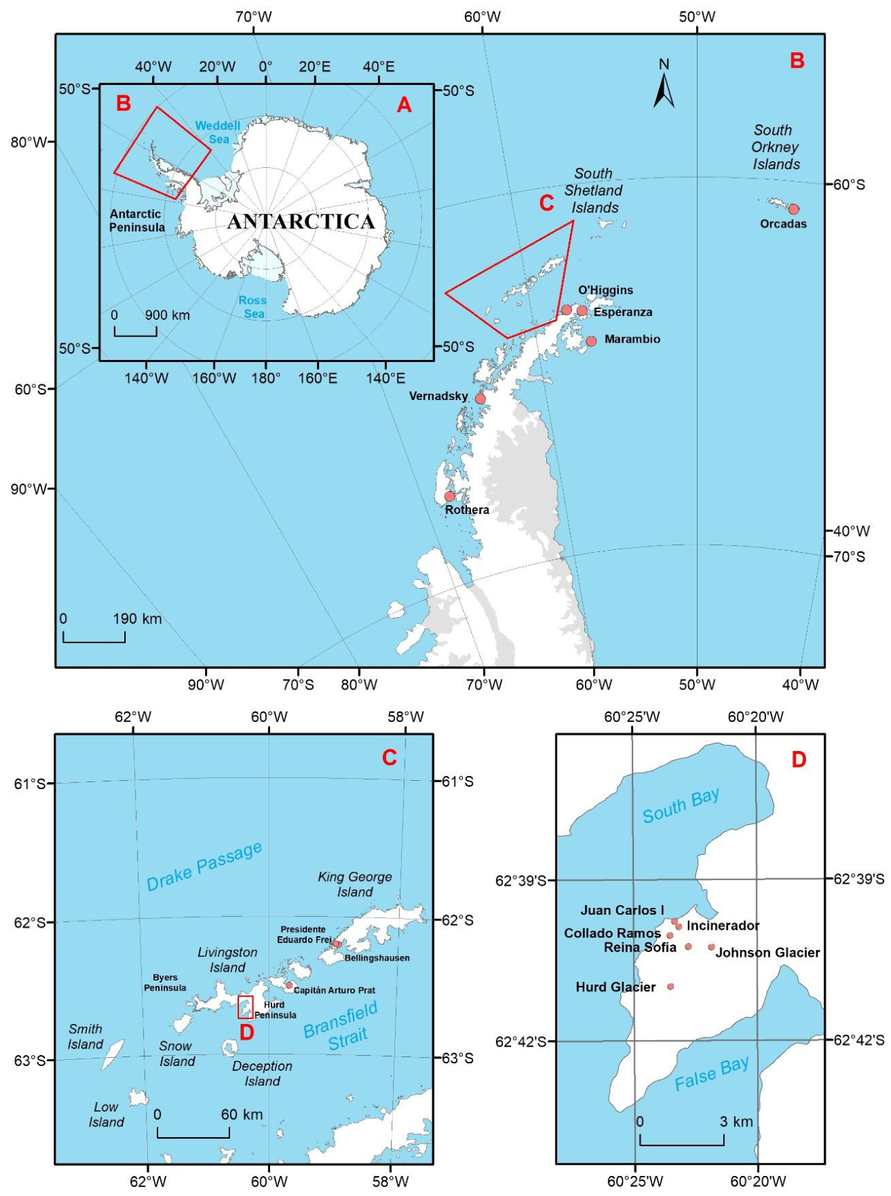
Figure 2.
MODIS filtering procedure for JCI as an example: (a) all observations separated by quality-control (QC) code; (b) good-quality observations (QC = 0 and QC = 8); and (c) good-quality observations with |view angle| ≤ 45°, corresponding to the final filtered MODIS data used in this study.
Figure 2.
MODIS filtering procedure for JCI as an example: (a) all observations separated by quality-control (QC) code; (b) good-quality observations (QC = 0 and QC = 8); and (c) good-quality observations with |view angle| ≤ 45°, corresponding to the final filtered MODIS data used in this study.
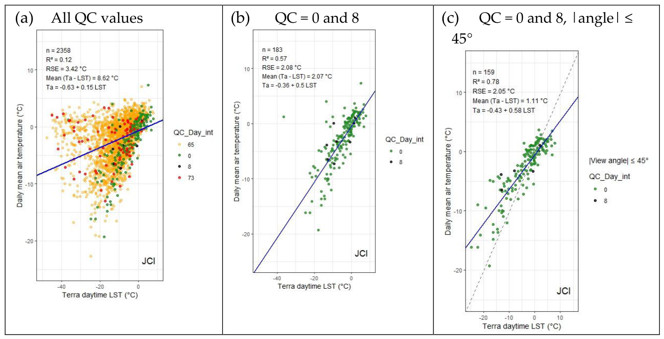
Figure 3.
Time series of daily mean Ta at AEMET stations. The fitted linear trend, significant at JCI and HG, is shown in red (see Table 5).
Figure 3.
Time series of daily mean Ta at AEMET stations. The fitted linear trend, significant at JCI and HG, is shown in red (see Table 5).
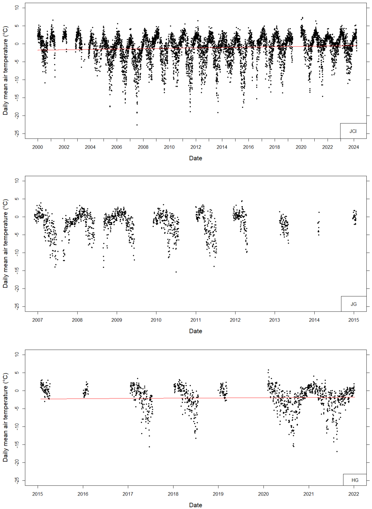
Figure 4.
Time series of daily mean Ta at PERMATHERMAL stations. The fitted linear trend for each series is shown in red (see Table 5).
Figure 4.
Time series of daily mean Ta at PERMATHERMAL stations. The fitted linear trend for each series is shown in red (see Table 5).
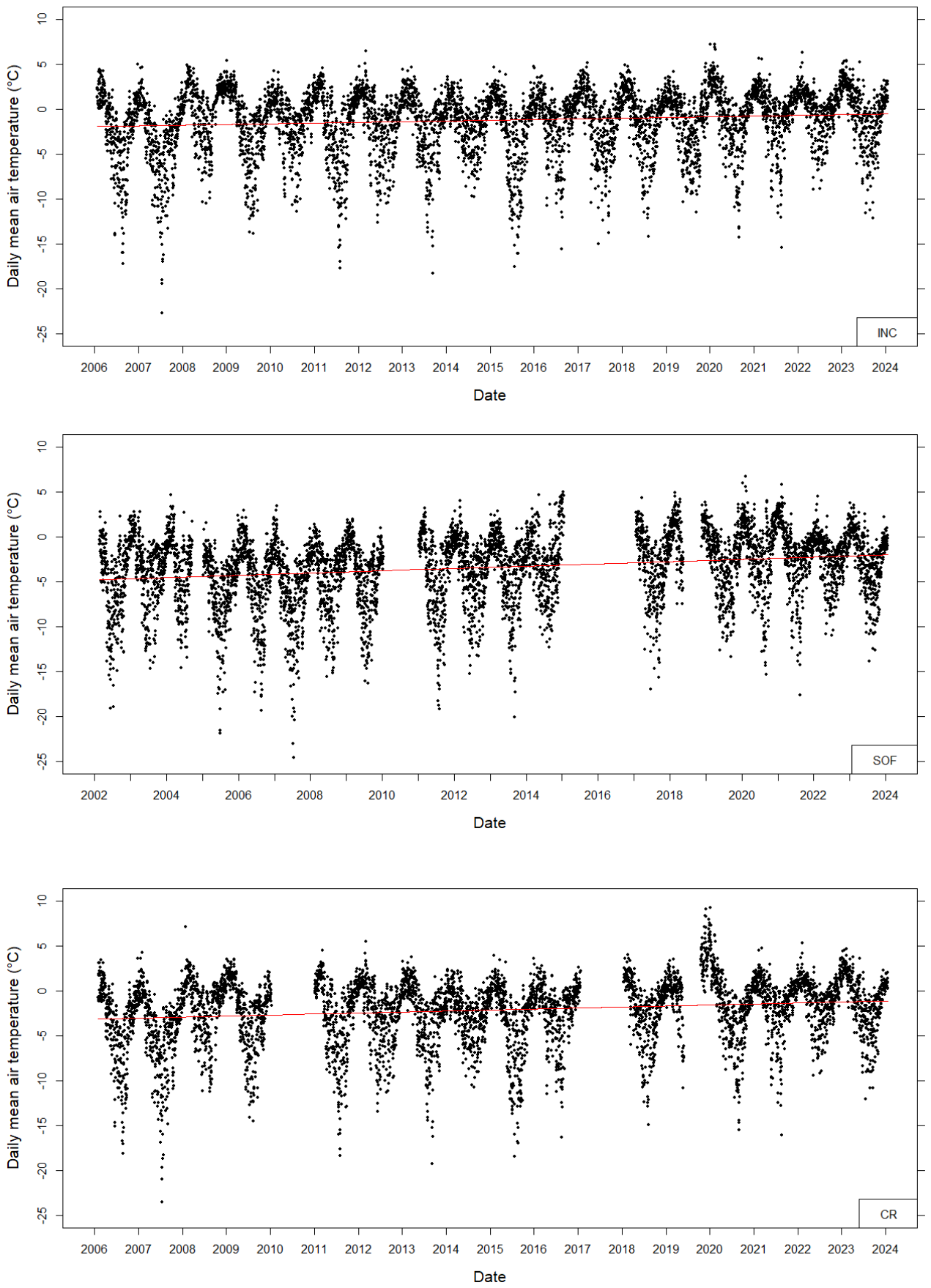

Table 1.
Name, current location, height above sea level (h), and operation dates since 2000 of the AEMET stations used in this study.
Table 1.
Name, current location, height above sea level (h), and operation dates since 2000 of the AEMET stations used in this study.
| AEMET station | Latitude | Longitude | h (m) | Operation dates (since 2000) |
|---|---|---|---|---|
| Juan Carlos I (JCI) |
62°39’48’’S | 60°23’19’’W | 13 | 01/January/2000 Present |
| Johnsons Glacier (JG) |
62°40’16’’S | 60°21’51’’W | 178 | 01/December/2006 24/January/2015 |
| Hurd Glacier (HG) |
62°41’48’’S | 60°24’44’’W | 93 | 25/January/2015 Present |
Table 2.
Name, current location, height above sea level (h), and operation dates since 2000 of the PERMATHERMAL stations. Note: although data collection at INC and SOF began in 2000, the initial years were excluded from the analysis, as explained in the text. Therefore, the actual start dates of the study period for each station are indicated in Table 5.
Table 2.
Name, current location, height above sea level (h), and operation dates since 2000 of the PERMATHERMAL stations. Note: although data collection at INC and SOF began in 2000, the initial years were excluded from the analysis, as explained in the text. Therefore, the actual start dates of the study period for each station are indicated in Table 5.
| PERMATHERMAL station |
Latitude | Longitude | h (m) | Operation dates (since 2000) |
|---|---|---|---|---|
| Incinerador (INC) |
62°39’53’’S | 60°23’08’’W | 34 |
25/February/2000 Present |
| Reina Sofía (SOF) |
62°40’16’’S | 60°22’46’’W | 271 |
25/February/2000 Present |
| Collado Ramos (CR) |
62°40’03’’S | 60°23’32’’W | 117 | 2/February/2006 Present |
Table 3.
Percentage distribution of MODIS Terra daytime LST quality-control (QC) codes for each meteorological station, together with the corresponding integer and binary QC codes and their quality information. QC-code descriptions adapted from Wan [47]. The number of available simultaneous Ta–LST observations (n) is indicated for each station.
Table 3.
Percentage distribution of MODIS Terra daytime LST quality-control (QC) codes for each meteorological station, together with the corresponding integer and binary QC codes and their quality information. QC-code descriptions adapted from Wan [47]. The number of available simultaneous Ta–LST observations (n) is indicated for each station.
| QC_Day_int with LST data |
JCI n=2358 |
JG n=481 |
HG n=202 |
INC n=2182 |
SOF n=2437 |
CR n=1641 |
|---|---|---|---|---|---|---|
| 0 | 7.4% | 6.4% | 2.0% | 7.2% | 5.6% | 6.2% |
| 8 | 0.3% | 1.9% | 0% | 0.3% | 0.4% | 0.1% |
| 65 | 88.3% | 82.7% | 96.5% | 88.5% | 86.4% | 90.6% |
| 73 | 4.0% | 8.9% | 1.5% | 4.0% | 7.6% | 3.1% |
Table 4.
Topographic variables and distance to the coast at the station locations from AW3D30 at the station locations.
Table 4.
Topographic variables and distance to the coast at the station locations from AW3D30 at the station locations.
| Station |
Slope | Roughness | Curvature (m-1) |
Orientation (radians) |
Distance to the coast (m) |
|---|---|---|---|---|---|
| JCI | 0.0018 | 0.000045 | -0.004444 | 5.136 | 88 |
| JG | 0.0524 | 0.000033 | -0.002222 | 0.423 | 950 |
| HG | 0.2050 | 0.000901 | 0.013333 | 4.011 | 291 |
| INC | 0.5146 | 0.008773 | -0.007778 | 5.527 | 266 |
| SOF | 0.2900 | 0.011546 | 0.023333 | 2.464 | 1020 |
| CR | 0.0299 | 0.001293 | 0.008889 | 4.173 | 420 |
Table 5.
Results of the model fitted using Equation (1) to the daily mean Ta series at each station for three different time periods (from top to bottom): 2000–2024, 2000–2015, and 2016–2024. The final column shows the initial and final temperatures (Tinitial and Tfinal) and the corresponding change in Ta (ΔTa) over the years indicated for each series, based solely on the linear trend.
Table 5.
Results of the model fitted using Equation (1) to the daily mean Ta series at each station for three different time periods (from top to bottom): 2000–2024, 2000–2015, and 2016–2024. The final column shows the initial and final temperatures (Tinitial and Tfinal) and the corresponding change in Ta (ΔTa) over the years indicated for each series, based solely on the linear trend.
| Station | Time period for Ta model |
Ta model (Equation (1)) |
n | R2 | RSE (°C) |
Ta – linear trend Tini, Tfin, ΔTa (°C) in years |
|---|---|---|---|---|---|---|
| JCI | 01-Jan-2000/ 23-Mar-2024 |
Ta = (-107.9612) +(0.0531) t + (1.5282) sin2πt +(2.8121) cos2πt |
7252 | 0.48 | 2.1 | -1.761, -0.475 +1.286 in 24.224 |
| JG | 02-Dec-2006/ 24-Jan-2015 |
Ta = (-2.3716) + (0.6002) sin2πt +(2.7869) cos2πt |
1423 | 0.41 | 2.0 |
Not applicable t is not significant |
| HG | 25-Jan-2015/ 07-Jan-2022 |
Ta = (-136.6867) + (0.0667) t + (1.3095) sin2πt +(2.4521) cos2πt |
1228 | 0.45 | 1.9 | -2.282, -1.818 +0.464 in 6.950 |
| INC | 24-Jan-2006/ 21-Jan-2024 |
Ta = -158.1895) + (0.0779) t + (1.5032) sin2πt +(2.6935) cos2πt |
6536 | 0.45 | 2.2 | -1.917, -0.516, +1.402 in 17.992 |
| SOF | 23-Feb-2002/ 21-Jan-2024 |
Ta = (-259.4494) + (0.1272) t + (1.4634) sin2πt +(2.9728) cos2πt |
6555 | 0.45 | 2.7 | -4.777 -1.990 +2.787 in 21.910 |
| CR | 02-Feb-2006/ 21-Jan-2024 |
Ta = (-229.8234) + (0.1130) t + (1.5597) sin2πt +(2.7086) cos2πt |
5680 | 0.47 | 2.2 | -3.135, -1.105 +2.030 in 17.967 |
| JCI | 01-Jan-2000/ 31-Dec-2015 |
Ta = (74.8058) +(-0.0380) t + (1.5437) sin2πt +(2.9663) cos2πt |
4752 | 0.48 | 2.2 | -1.194 - 1.802 -0.608 in 15.997 |
| JG | 02-Dec-2006/ 24-Jan-2015 |
Ta = (-2.3716) + (0.6002) sin2πt +(2.7869) cos2πt |
1423 | 0.41 | 2.0 |
Not applicable t is not significant |
| HG | 25-Jan-2015/ 10-Apr-2015 |
Not applicable Limited data |
75 | 0.27 | - |
Not applicable Limited data |
| INC | 24-Jan-2006/ 31-Dec-2015 |
Ta = (-1.5221) + (1.5687) sin2πt +(2.9140) cos2πt |
3596 | 0.45 | 2.4 |
Not applicable t is not significant |
| SOF | 23-Feb-2002/ 20-Jan-2015 |
Ta = (-178.5434) + (0.0869) t + (1.4314) sin2πt +(3.1232) cos2πt |
4186 | 0.41 | 2.8 | -4.557, -3.435 +1,122 in 12.907 |
| CR | 02-Feb-2006/ 31-Dec-2015 |
Ta = (-80.0419) + (0.0385) t + (1.8049) sin2πt +(2.9062) cos2πt |
3240 | 0.46 | 2.4 | -2.808, -2.426 +0.381 in 9.909 |
| JCI | 01-Jan-2016/ 23-Mar-2024 |
Ta = (-158.2466) +(0.0782) t + (1.3884) sin2πt +(2.3391) cos2πt |
2500 | 0.48 | 1.7 | -0.595, +0.048 + 0.643 in 8.224 |
| HG | 05-Jan-2016/ 07-Jan-2022 |
Ta = (-265.1349) + (0.1303) t + (1.3606) sin2πt +(2.4291) cos2πt |
1153 | 0.44 | 2.0 | -2.449, -1.666 +0.782 in 6.005 |
| INC | 01-Jan-2016/ 21-Jan-2024 |
Ta = (-269.3359) + (0.1330) t + (1.4193) sin2πt +(2.4389) cos2πt |
2940 | 0.46 | 2.0 | -1.208, -0.137, +1.071 in 8.055 |
| SOF | 24-Jan-2017/ 21-Jan-2024 |
Ta = (-82.3048) + (0.0396) t + (1.4292) sin2πt +(2.7218) cos2π t |
2369 | 0.44 | 2.4 | -2.429, -2.152 +0.276 in 6.992 |
| CR | 01-Jan-2016/ 21-Jan-2024 |
Ta = (-253.7903) + (0.1249) t + (1.2466) sin2πt + (2.4340) cos2πt |
2440 | 0.44 | 2.0 | -1.992, -0.986 +1.006 in 8.055 |
Table 6.
Slope (α) of the linear trend at each station for the three study periods. Notes: Italicized values for HG are based on shorter available records (2015–2022 and 2016–2022) and should be interpreted with caution. 0* indicates that the time variable (t) was not statistically significant (p > 0.05).
Table 6.
Slope (α) of the linear trend at each station for the three study periods. Notes: Italicized values for HG are based on shorter available records (2015–2022 and 2016–2022) and should be interpreted with caution. 0* indicates that the time variable (t) was not statistically significant (p > 0.05).
| Station | h (m) |
2000-2024 α (°C decade−1) |
2000-2015 α (°C decade−1) |
2016-2024 α (°C decade−1) |
|---|---|---|---|---|
| JCI | 13 | 0.53 | -0.38 | 0.78 |
| INC | 34 | 0.78 | 0* | 1.33 |
| HG | 93 | 0.67 | - | 1.30 |
| CR | 117 | 1.13 | 0.39 | 1.25 |
| SOF | 271 | 1.27 | 0.87 | 0.40 |
Table 7.
Model for estimating Ta from MODIS Terra daytime LST using data from all six stations. The structure is Ta = c1 + c2 LST + c3 t + c4 sin 2πt + c5 cos 2πt + c6 H + c7 l + c8 r + c9 c, with Ta and LST in °C, t in decimal year units, H in hours, longitude (l) in degrees, roughness (r; dimensionless), and curvature (c) in m−1.
Table 7.
Model for estimating Ta from MODIS Terra daytime LST using data from all six stations. The structure is Ta = c1 + c2 LST + c3 t + c4 sin 2πt + c5 cos 2πt + c6 H + c7 l + c8 r + c9 c, with Ta and LST in °C, t in decimal year units, H in hours, longitude (l) in degrees, roughness (r; dimensionless), and curvature (c) in m−1.
| MODIS Data | n | R2 | RSE (°C) |
c1 (°C) | c2 (LST) | c3 (t) | c4 (sin) | c5 (cos) | c6(H) | c7 (l) | C8 (r) | c9 (c) |
|---|---|---|---|---|---|---|---|---|---|---|---|---|
| Terra-Day | 568 | 0.77 | 1.52 | 444 ± 651 |
0.65 ± 0.02 |
0.101 ± 0.014 |
0.18 ± 0.11 |
-1.29 ± 0.20 |
-0.99 ± 0.19 |
-11 ± 11 |
-57 ± 17 |
-41 ± 7 |
Table 8.
Leave-one-out cross-validation of the global MODIS Terra-Day model.
| MODIS Data | n | R2CV | RMSECV (°C) | MAE (°C) | RPD | Bias (°C) |
|---|---|---|---|---|---|---|
| Terra-Day | 568 | 0.75 | 2.23 | 1.51 | 2.00 | 0.05 |
Disclaimer/Publisher’s Note: The statements, opinions and data contained in all publications are solely those of the individual author(s) and contributor(s) and not of MDPI and/or the editor(s). MDPI and/or the editor(s) disclaim responsibility for any injury to people or property resulting from any ideas, methods, instructions or products referred to in the content. |
© 2026 by the authors. Licensee MDPI, Basel, Switzerland. This article is an open access article distributed under the terms and conditions of the Creative Commons Attribution (CC BY) license (http://creativecommons.org/licenses/by/4.0/).
Copyright: This open access article is published under a Creative Commons CC BY 4.0 license, which permit the free download, distribution, and reuse, provided that the author and preprint are cited in any reuse.