

Submitted:
24 September 2026
Posted:
24 September 2026
You are already at the latest version
Abstract
Total suspended matter (TSM) is a key coastal water-quality indicator, yet the operational GOCI-II retrieval algorithm is constrained by an empirical ceiling of approximately 28.13 g m⁻³ because of the inherent dynamic-range limitation of visible band-ratio formulations in the current operational product; this limitation precludes accurate monitoring of turbid nearshore environments, which is critical for ecosystems and coastal management. Here, we developed and evaluated a physically interpretable stacking ensemble (PISE) model that fuses three complementary base learners via a ridge meta-learner on five physically interpretable GOCI-II Rᵣₛ (555, 620, 709 nm) features trained on 212 matchup samples (2022–2025). On an independent held-out test set, PISE achieves R² = 0.793 and RMSE = 3.670 g m⁻³, improving the operational GOCI-II product by 8.9 percentage points in R² and 16.3% in RMSE, with 90% conformal prediction intervals achieving 90.6% empirical coverage. On 4 May 2025 GOCI-II imagery, PISE captures the Gyeonggi Bay flood-ebb TSM cycle, with a +0.006 g m⁻³ per cm regression against the KHOA tidal-stage gauge. PISE thereby provides a quantitative satellite-derived characterization of diurnal TSM dynamics across the flood-ebb tidal cycle over Korean coastal waters, extending operational TSM retrieval above the 28.13 g m⁻³ retrieval ceiling up to its trained limit of 50 g m⁻³.
Keywords:
total suspended matter
; Geostationary Ocean Color Imager-II
; stacking ensemble
; machine learning
; Korean coastal waters
1. Introduction
Coastal water optics are governed by phytoplankton, colored dissolved organic matter, and mineral suspended sediment, the last of which dominates turbid nearshore zones [1,2]. Mineral sediment controls light availability for benthic photosynthesis, modulates phytoplankton production, and carries adsorbed nutrients and contaminants across the land–ocean interface [3,4,5]. In macrotidal shelves, such as the Yellow Sea, total suspended matter (TSM) spans three to four orders of magnitude within a few kilometers, from oligotrophic waters below 0.1 g m⁻³ to turbid nearshore zones exceeding 50 g m⁻³ [6,7,8]. Satellite ocean color remote sensing is the only platform that can monitor this variability at the resolution that operational coastal management requires [3,9,10]. Established semianalytical and empirical TSM algorithms using visible and near-infrared reflectance [4,5] have been validated globally, yet their performance on the turbid, macrotidal Yellow Sea coast remains constrained by the algorithm dynamic range and atmospheric correction uncertainty [11,12].
TSM retrieval algorithms have followed two broad approaches. Empirical band-ratio and regression algorithms relate one or two reflectance bands directly to in situ TSM through local calibration [3,4]; they are simple to implement and robust within their calibration range but transfer poorly to water types or sediment mineralogies outside it. Semianalytical algorithms instead invert reflectance through backscattering models grounded in inherent optical property theory [4,5,31], improving generality at the cost of requiring accurate a priori assumptions about particle optical properties. Both approaches require regional recalibration for the Yellow Sea and adjacent Chinese and Korean shelf waters [6,52], reflecting the difficulty of a single global algorithm capturing the mineralogical and hydrodynamic complexity of this system.
The Geostationary Ocean Color Imager (GOCI), the world’s first geostationary ocean color sensor, operated over the Korean peninsula from 2011 to 2021, establishing that hourly revisits could resolve a range of coastal dynamics from suspended sediment fronts to photosynthetically available radiation [7,8,13,14,15,16], with independently verified Rᵣₛ accuracy across the visible bands over Korean waters [19]. Its successor, GOCI-II, extends this capability from ∼36 000 km altitude at 250 m resolution across 12 spectral bands [20,21]. GOCI-II’s operational TSM product retains the empirical band-ratio design of its predecessor, deriving TSM from a power-law relationship between Rᵣₛ(555) and Rᵣₛ(620) calibrated against Korean coastal in situ data [22]; ongoing algorithm development for this product has identified the high-turbidity regime as a specific area requiring improvement [20]. Because this visible band-ratio formulation has an inherent dynamic range limitation at high mineral concentrations, an effective empirical ceiling of 28.13 g m⁻³ [22,23] constrains retrieval in exactly the turbid nearshore zones that are ecologically and hydrodynamically most dynamic in the Yellow Sea system.
This ceiling matters most for diurnal monitoring, which is the specific objective of the present study. Prior work exploiting geostationary revisits to resolve subdaily TSM dynamics—He et al. [17] and Hu et al. [18] over Chinese and Korean shelf waters and Neukermans et al. [51] adapting the non-ocean-color-optimized SEVIRI meteorological sensor over the southern North Sea—relied on single-band empirical or semianalytical algorithms whose dynamic range was fixed by their original calibration data rather than by the demands of tracking turbidity fronts through a full tidal cycle. Ruddick et al. [50,55] identify this mismatch between the algorithm dynamic range and the requirements of high-frequency turbid-water monitoring as a persistent constraint on geostationary ocean color, which is most acute precisely where diurnal variability is greatest. These studies used the algorithms available to them because none offered comparable operational simplicity and computational speed for hourly, basin-scale processing; extending the dynamic range without sacrificing operational tractability motivates the machine learning approach developed here.
Machine learning (ML) offers a route for extending the algorithm’s dynamic range without making new physical assumptions about particle optics. For TSM and total suspended solids specifically, ML approaches incorporating water-type classification and semianalytical priors have outperformed single-band empirical algorithms across a concentration range spanning clear to hypertidal turbid waters [10], and gradient boosting [27] and related tree ensemble methods [28,29] perform robustly in optically complex coastal waters where standard atmospheric correction and semianalytical inversion struggle [10,26]. These gains are not unconditional: ML models trained on imbalanced or geographically restricted matchup datasets can produce overoptimistic performance estimates under naive cross-validation and generalize poorly outside their training distribution [35,36], a limitation that in principle affects any data-driven retrieval algorithm, including the one developed here. Among ensemble architectures, stacked generalization [30] offers a principled framework for combining base learners with complementary inductive biases through a regularized meta-learner, reducing variance without sacrificing each constituent model’s accuracy gains. Despite these developments, stacking with physically interpretable spectral features has not been applied to GOCI-II TSM retrieval, existing ML approaches for this sensor and variable have not addressed its empirical retrieval ceiling, and none have provided calibrated pixel-level uncertainty estimates. Here, ‘Physically interpretable’ refers to deriving all five input features from established optical scattering theory for turbid waters [4,31] and constraining the feature space to physically meaningful reflectance transformations rather than raw band values or purely data-driven selection. Section 5.1 evaluates this claim directly against in situ backscattering measurements. Conformal prediction [32,33] offers a distribution-free framework for prediction intervals with finite-sample marginal coverage guarantees requiring no distributional assumptions, yet its application to satellite ocean color TSM retrieval remains, to our knowledge, unexplored.
The overarching objective of this study is to develop and validate PISE, a physically interpretable stacking ensemble that resolves diurnal TSM dynamics over Korean coastal waters beyond the dynamic-range limits of existing GOCI-II and geostationary algorithms. Three specific objectives support this goal: (1) to apply PISE to a full day of GOCI-II imagery to characterize diurnal TSM dynamics relative to tidal forcing, extending the geostationary diurnal monitoring work of He et al. [17], Hu et al. [18], and Ruddick et al. [50,51,55] to the empirical ceiling-exceeding concentration range; (2) to characterize the methodological contributions of the ensemble by quantifying the roles of individual base learners and spectral features through ablation and permutation importance analysis [28,34] and by providing calibrated pixel-level uncertainty estimates through split conformal prediction [32,33]; and (3) to rigorously evaluate PISE’s temporal and spatial generalization through nested leave-year-out and spatial block cross-validation [35,36].
2. Materials and Methods
2.1. Study Area
The study domain spans 124–130°E and 32–38°N across the western and southern Korean coastal waters (Figure 1), one of the world’s most energetic macrotidal shelves: M2 tidal ranges in Gyeonggi Bay regularly exceed 9 m [37], and the tidal currents there are strong enough to sustain a permanently turbid bottom nepheloid layer along the inner western coast [7,37]. The Yellow Sea Warm Current supplies clearer oceanic water to the outer shelf in summer, although its pathway varies seasonally and interannually [38,39], while freshwater discharge from the Han and Geum Rivers drives seasonal TSM gradients along the northern and central west coasts. Suspended sediment in the domain is among the highest in any shelf sea worldwide, with provenance studies tracing the dominant mineral fraction to Chinese and Korean river inputs transported northward by residual tidal currents [6]; in situ TSM ranges from less than 0.1 g m⁻³ in the central Yellow Sea to frequently exceed 20 g m⁻³ in Gyeonggi Bay and along the South Jeolla coast [7,8].
Three regions of interest (ROIs) represent distinct turbidity regimes: the Mokpo Coast (126.2–126.7°E, 34.6–34.9°N) is a persistently high-turbidity environment that is well characterized by GOCI-based monitoring [7,8] where tidal energy sustains well-mixed sediment concentrations near 20 g m⁻³ year-round; Gyeonggi Bay (126.0–126.8°E, 36.8–37.4°N) shows strong tidal modulation of TSM tracking the flood-ebb cycle ([8,37]; Section 4.3); and Jeju Offshore (126.0–127.0°E, 33.0–33.5°N) is a clear-water reference site with TSM consistently below 1 g m⁻³.
2.2. Dataset
GOCI-II Level-1B (L1B) top-of-atmosphere radiance is processed operationally to Level-2 (L2) remote-sensing reflectance (Rᵣₛ) by the GOCI-II Ground Segment (G2GS), whose atmospheric correction follows the algorithm originally developed for the GOCI/GOCI-II sensor series by Ahn and colleagues [13,20], most recently updated (v2024-1) with sensor-degradation correction, revised vicarious calibration gains, and the spectral relationship of inherent optical properties (SRIOP) red-NIR method for highly turbid waters [23,44]. In this study, the resulting operational G2GS L2 Rᵣₛ product is used as the sole satellite input to PISE.
In situ TSM was measured aboard KIOST research vessels following the KOSC/KIOST validation protocol [40,41]: triplicate seawater subsamples (0.1–1.0 L) were vacuum-filtered (≤ 250 mmHg) through preweighed 47-mm polycarbonate filters (0.4 µm), rinsed with 15 mL of Milli-Q water to remove residual sea salts, dried at 60 °C for 4 h before and after filtration, and weighed to 0.01 mg with blank-filter drift correction; station TSM was calculated from the difference in the blank-corrected mass divided by the filtered volume, which is consistent with established ocean-color validation practice [42,43].
Matchups used a 3×3 pixel extraction window with coefficient-of-variation filtering (CV < 0.15) to exclude heterogeneous scenes [14,15] and a ±30 min temporal window, exploiting GOCI-II’s geostationary revisit to minimize atmospheric and oceanic variability between overpass and in situ sampling.
The PISE matchup dataset consists of 212 satellite-in situ pairs collected between January 2022 and March 2025 (Table 1). Three GOCI-II Rᵣₛ bands are used as model inputs: 555, 620, and 709 nm. These bands were selected because they jointly span the spectral region of maximum sensitivity to mineral particle backscattering in turbid coastal waters: 555 nm anchors the green reflectance peak used by standard TSM band-ratio algorithms [4], 620 nm is the red‒orange channel that is most strongly and linearly responsive to suspended-sediment backscattering across the full concentration range [2,31], and 709 nm extends this sensitivity toward the red-edge/NIR transition, where reflectance does not saturate at high TSM and where the SRIOP atmospheric correction provides the most reliable retrieval in turbid waters [44]. The 745 nm band is excluded because its operational value is partly derived from the 620 nm and 709 nm channels during atmospheric correction and therefore does not constitute an independent observable [20,21]. The in situ TSM ranges from 0.07 to 51.33 g m⁻³, with a median of 1.30 g m⁻³. The dataset is heavily right-skewed: 40.1 % of the samples have a TSM < 1 g m⁻³, 36.3 % fall in the 1–5 g m⁻³ range, 18.4 % in the 5–20 g m⁻³ range, and the remaining 5.2 % (n = 11) exceed 20 g m⁻³. This distribution is characteristic of matched coastal datasets dominated by clear-water samples [4,9]. The temporal, spatial, and statistical distributions are summarized in Figure 2.
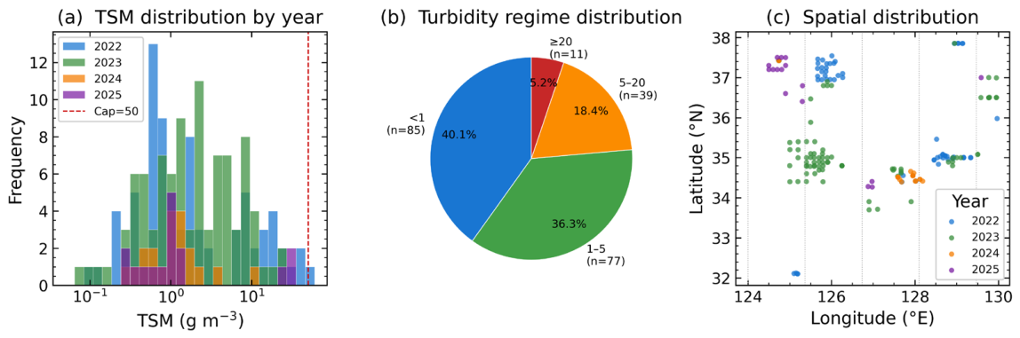
Figure 2.
Dataset overview: (a) histogram of in situ TSM by year; (b) pie chart of the turbidity regime distribution (clear: TSM < 1; low: 1–5; medium: 5–20; high: > 20 g m⁻³); (c) spatial scatter of matchup locations across the study domain.
Figure 2.
Dataset overview: (a) histogram of in situ TSM by year; (b) pie chart of the turbidity regime distribution (clear: TSM < 1; low: 1–5; medium: 5–20; high: > 20 g m⁻³); (c) spatial scatter of matchup locations across the study domain.

Table 1.
Summary statistics for the 212-sample GOCI-II satellite-in situ matchup dataset.
| Parameter | Value |
| Total matchup pairs | 212 |
| Collection period | January 2022 – March 2025 |
| Temporal matchup window | ±30 min |
| Spatial matchup window | 3×3 pixel, CV < 0.15 |
| TSM range (g m⁻³) | 0.07 – 51.33 |
| TSM median (g m⁻³) | 1.30 |
| Training set (n) | 148 (70 %) |
| Test set (n) | 64 (30 %) |
| GOCI-II bands used | Rᵣₛ(555), Rᵣₛ(620), Rᵣₛ(709) nm |
For model training and evaluation, the target variable TSM was winsorized before log-transformation to define the upper boundary of the model’s valid retrieval range. The current in situ matchup dataset does not sample the extremely turbid water environments characteristic of the Yellow Sea and Mokpo coastal zone, where TSM is known to reach 150–200 g m⁻³ during maximum tidal flux [6,7,8]. In the absence of training data representing those concentrations, a winsorization cap of 50 g m⁻³ was applied as a physical necessity to ensure stable meta-learner training and prevent extrapolation beyond the dataset’s representable concentration range. The applied cap influences only the single sample with TSM > 50 g m⁻³ and acts as the operational upper bound of PISE retrievals throughout this study.
2.3. Preliminary Spectral Characterization
The empirical relationship between the satellite Rᵣₛ and in situ TSM is strongest at 620 nm (Pearson r ≈ 0.90 in log space), which is consistent with the dominant role of mineral particle backscattering in the red spectral region [4,31], followed by the relationships at 555 nm (r ≈ 0.87) and 709 nm (r ≈ 0.85; Figure 3). Rᵣₛ spectra separate clearly by turbidity regime, with high-turbidity samples showing both elevated magnitude and the spectral redshift characteristic of mineral-dominated backscattering [2,31], confirming the suitability of these three bands for the engineered features described in Section 2.4.
2.4. Physically Interpretable Spectral Features
Five physically interpretable spectral features are derived from the three GOCI-II Rᵣₛ bands (Table S1). Log compression of the dynamic range is among the most effective preprocessing steps for ocean color TSM retrieval across multidecade concentration ranges [4,5,10]. The spectral difference and band ratio features exploit the differential sensitivity of the red and red-edge/NIR channels to mineral particle backscattering: in mineral-dominated turbid waters, the backscattering spectrum shows a well-documented red spectral shift with increasing sediment concentration, making the spectral difference between visible and red-NIR bands a physically grounded TSM proxy [2,31] (Table S1).
The spectral difference f₄ captures the redshift in backscattering with increasing mineral sediment concentration [4,31]. The band ratio f₅ is a backscattering index that is largely independent of pigment variation, following the NIR-based backscattering framework for turbid coastal waters [2], and serves as the primary semianalytical TSM proxy in the current GOCI-II Algorithm Theoretical Basis Document (ATBD) [22].
The term ‘physically interpretable’ refers to the bio-optical basis on which the five input features were constructed (Figure 4), not to radiative transfer operators embedded within the model architecture. Feature selection followed established ocean optics principles: the progressive redshift of the reflectance peak with increasing particle concentration motivates the spectral difference f₄ and band ratio f₅, whereas the log transformations in f₁–f₃ encode the known power-law relationship between particulate backscattering and Rᵣₛ. The retrieval bands were chosen because their optical sensitivity to mineral particles in turbid coastal waters is documented extensively in the literature [4,31]. The conformal prediction intervals and permutation feature importance results further make the ensemble’s predictions and feature contributions traceable to physical and statistical principles. This feature-engineering strategy, which is grounded in bio-optical theory rather than purely statistical variable selection, distinguishes PISE from unconstrained black-box machine learning approaches.
2.5. Winsorization and Cap Selection
where y is the measured in situ TSM and c = 50 g m⁻³ is the cap, selected via the sensitivity analysis in Section 2.5. The winsorized target is transformed as y∗ = ln(1 + ỹ) (log1p), and predictions are back-transformed at inference as ŷ = exp(ŷ∗) − 1 (expm1).
2.6. Model Architecture
Ensemble formulation. PISE combines three base learners through a Ridge meta-learner using stacked generalization ([30]; Eq. 2):
where x (= [f₁, f₂, f₃, f₄, f₅]ᵀ) is the feature vector and fGB, fSVR, and fBR are the gradient boosting (GB) [27], support vector regression (SVR) [45], and Bayesian ridge (BR) [46] base learners, respectively. All the components are implemented in scikit-learn [47].
Base learners. Gradient boosting [27] is the workhorse tree-boosting algorithm underlying the widely used XGBoost framework [29]; we use the scikit-learn implementation with 300 trees, a maximum depth of 4, a learning rate of 0.05, and a minimum of 10 samples per leaf. Support vector regression [45] uses a radial basis function kernel (C = 10, γ = scale) with RobustScaler preprocessing to handle the heavy-tailed Rᵣₛ distribution in turbid waters. Bayesian ridge [46] is a fully probabilistic linear base learner that regularizes toward the prior mean, adding model diversity complementary to the tree- and kernel-based learners.
Meta-learner and out-of-fold procedure. The ridge meta-learner uses α = 5.0, chosen by 5-fold cross-validation on the training set. Meta-features are generated via out-of-fold prediction [30]: for each fold of a 5-fold training split, each base learner is trained on four folds and predicts the held-out fifth, preventing data leakage into the meta-learner.
2.7. Validation Framework
Held-out test set. The 212 samples were divided 70/30 into training (n = 148) and test (n = 64) sets using stratified sampling by year (random seed 42). The test set is withheld until the final evaluation and is the primary basis for all headline comparisons (Table 2, Figure 5).
Nested leave-year-out (LYO) cross-validation. PISE is retrained from scratch with one calendar year withheld and then evaluated on that withheld year. This protocol tests strict temporal extrapolation and follows the temporal blocking strategy recommended for structured environmental data [35,36]. The four LYO folds contain 82 (2022), 94 (2023), 20 (2024), and 16 (2025) samples.
Spatial block cross-validation. Four longitudinal blocks are used to divide the matchup domain: B0 (124–126°E, n = 102), B1 (126–127°E, n = 33), B2 (127–129°E, n = 37), and B3 (129–130°E, n = 40). This design avoids the overly optimistic error estimates that random partitioning produces in spatially autocorrelated datasets [35,36,48]. For each fold, PISE is trained on three blocks and evaluated on the fourth.
2.8. Uncertainty Quantification Via Conformal Prediction
Conformal prediction intervals. Split conformal prediction [32,33] provides a distribution-free 90% prediction interval (PI) with no distributional assumptions. A calibration set of n = 37 samples, withheld from all base-learner training and out-of-fold meta-feature generation, is used solely to compute nonconformity scores on genuinely held-out predictions, preserving the finite-sample marginal coverage guarantee of split conformal prediction [32,33]. The empirical quantile q̂ of the calibration absolute residuals is computed at level (1 − α)(1 + 1/nₐₐₗ) for α = 0.10, yielding the interval (Eq. 3):
2.9. Evaluation Metrics and Cap Sensitivity Protocol
Six winsorization caps (c ∈ {10, 20, 30, 40, 50, 60} g m⁻³) are evaluated to identify the optimal trade-off between training stability and retrieval accuracy at extreme concentrations. For each cap, the full PISE pipeline is retrained from scratch and evaluated on the held-out test set alongside the GOCI-II ATBD, following the assessment framework recommended by Seegers et al. [49].
Six metrics are computed for all the model comparisons, following the ocean color product evaluation framework of Seegers et al. [49] (Table S2): the coefficient of determination (R²), root mean square error (RMSE), mean absolute error (MAE), bias (mean signed deviation), symmetric mean absolute percentage error (SMAPE), and log-scale root mean square error (LogRMSE).
The 95% confidence intervals for R² are computed from 1,000 resamples of the test set.
3. Results
3.1. Overall PISE Performance and Operational Improvement
On the held-out test set (n = 64), PISE achieves R² = 0.793 (95% CI: 0.715, 0.934; the asymmetric interval reflects the positive skew of the R² bootstrap distribution near unity, expected for bootstrap resampling in this range), RMSE = 3.670 g m⁻³, MAE = 1.458 g m⁻³, Bias = −1.036 g m⁻³, SMAPE = 35.65%, and LogRMSE = 0.228 (defined in Table S2). The GOCI-II ATBD algorithm achieves R² = 0.704, RMSE = 4.385 g m⁻³, MAE = 1.806 g m⁻³, bias = −1.335 g m⁻³, and SMAPE = 43.25%. PISE outperforms GOCI-II on all six metrics, reducing the RMSE by 0.715 g m⁻³ (16.3%) and improving the R² by 0.089 (Table 2, Figure 5, Figure S10). Compared with the ocean color performance benchmarks of Seegers et al. [49], PISE’s 7.6-percentage-point SMAPE improvement confirms that the accuracy gain is proportionally consistent across the full concentration range.
Because the operational algorithm has no trainable parameters, a bootstrap CI for the GOCI-II ATBD is not applicable.
3.2. Cap Sensitivity Analysis and Empirical Evidence
The cap sensitivity experiment (Table 3, Figure 6, Figure S2 and Figure S11) is a deterministic test of the GOCI-II empirical retrieval ceiling. The GOCI-II R² and RMSE are identical to three decimal places at caps of 40, 50, and 60 g m⁻³ (R² = 0.704; RMSE = 4.385 g m⁻³), confirming that the operational algorithm cannot distinguish true concentrations above its 28.13 g m⁻³ ceiling. This identity arises mechanically: the 43.33 and 51.33 g m⁻³ samples both receive identical GOCI-II predictions capped at 28.13 g m⁻³, so including or excluding them does not change the operational algorithm’s statistics. PISE, by contrast, responds to the cap: performance is optimal at c = 50 g m⁻³ (R² = 0.793, RMSE = 3.670 g m⁻³). For the five samples above the GOCI-II ceiling (TSM > 28.13 g m⁻³), the maximum GOCI-II prediction is only 27.31 g m⁻³, whereas the in situ values reach 51.33 g m⁻³.
Caps below 40 g m−3 yield higher apparent R2 and lower RMSE only because they truncate the evaluated TSM range and discard genuine high-turbidity samples (e.g., cap = 10 retains just 186 of 212 points); among caps that preserve ≥99% of the dataset at true measured values (40, 50, and 60 g m−3), c = 50 minimizes RMSE and is therefore selected as optimal.
At cap = 50 g m⁻³, one sample (TSM = 51.33 g m⁻³) is winsorized to 50 g m⁻³ and retained; it is not excluded. The identical GOCI-II values at caps of 40–60 g m⁻³ confirm complete insensitivity above the 28.13 g m⁻³ empirical ceiling.
3.3. Base Learner and Feature Contributions: Overfitting and Ablation
PISE has a negative train-test gap (−0.043): its test-set R² (0.793) exceeds its training-set R² (0.750) (Figure 7), which is the expected signature of a well-regularized ensemble [27,30]. Among the base learners, gradient boosting shows a modest positive gap (+0.021), whereas SVR (−0.052) and Bayesian ridge (−0.127) generalize better on the test set, confirming that no base learner overfits the training distribution. An ablation study (Figure 7) reveals that gradient boosting alone achieves a test RMSE of 2.862 g m−3 but shows a persistent train-CV gap (+0.021). The stacking ensemble’s test RMSE is 0.808 g m−3 higher than GB alone (3.670 vs. 2.862 g m−3), but it eliminates that general-ization gap (−0.043) and generalizes more reliably across the base learners, which is the basis for selecting PISE over any single base learner
Permutation importance ([28,34]; Figure S3) identifies Rᵣₛ(620) as the dominant feature (ΔR² = 0.766), followed by Rᵣₛ(709) (ΔR² = 0.228), Rᵣₛ(555) (ΔR² = 0.149), the spectral difference f₄ (ΔR² = 0.041), and the band ratio f₅ (ΔR² = 0.023). The dominance of Rᵣₛ(620) is consistent with its established role as the primary mineral backscattering channel in turbid coastal waters [2,4,31].
3.4. Temporal and Spatial Generalization: Cross-Validation
Leave-year-out cross-validation. Table 4 and Figure S12 report the LYO results following the temporal blocking strategy of Roberts et al. [35]. PISE achieves R² = 0.489 and RMSE = 6.987 g m⁻³ for the 2022 fold (n = 82), and R² = 0.926 and RMSE = 0.589 g m⁻³ for the 2024 fold (n = 20). The 2023 fold is the most demanding: PISE R² = 0.253 versus GOCI-II R² = 0.525 when 2023 (n = 94, 44% of the training set) is withheld. The 2025 fold (n = 16) gives PISE R² = 0.833, interpreted cautiously given the small fold size.
Spatial block cross-validation. Table 4 and Figure S4 present spatial block results following Roberts et al. [35] and Valavi et al. [48]. B2 (127–129°E) is the best-performing block for PISE (R² = 0.902, RMSE = 0.533 g m⁻³). B1 (126–127°E) is most challenging for both models (PISE: R² = 0.156; GOCI-II: R² = 0.231), likely reflecting the optical complexity and high spatial heterogeneity of the inner Gyeonggi Bay and adjacent tidal flat environments [7,8].
Table 4.
Cross-validation results: nested leave-year-out (LYO) and spatial block cross-validation [35,48]. Bold values indicate better performance per fold. Units of the RMSE are g m⁻³.
| Fold | n | PISE R² | GOCI-II R² | PISE RMSE | GOCI-II RMSE |
| Nested leave-year-out (LYO) cross-validation | |||||
| 2022 | 82 | 0.489 | 0.506 | 6.987 | 6.873 |
| 2023 | 94 | 0.253 | 0.525 | 3.905 | 3.113 |
| 2024 | 20 | 0.926 | 0.876 | 0.589 | 0.764 |
| 2025 | 16 | 0.833 | 0.941 | 4.172 | 2.487 |
| Spatial block cross-validation | |||||
| B0 (124–126°E) | 102 | 0.675 | 0.551 | 3.558 | 4.185 |
| B1 (126–127°E) | 33 | 0.156 | 0.231 | 10.055 | 9.596 |
| B2 (127–129°E) | 37 | 0.902 | 0.838 | 0.533 | 0.687 |
| B3 (129–130°E) | 40 | 0.455 | 0.561 | 1.277 | 1.146 |
3.5. Uncertainty Calibration Via Conformal Prediction
The split conformal prediction intervals [32,33] achieve 90.6% empirical coverage on the test set, confirming that calibration within the finite-sample tolerance is guaranteed by conformal theory (Figure 8). The empirical quantile q̂ = 3.04 g m⁻³ defines the symmetric interval half-width, and the intermodel spread correlates with the actual absolute error at r = 0.661, providing a spatially variable secondary uncertainty signal. The permutation sanity check (Figure 8b; [34]) confirms that randomly permuted feature vectors achieve a maximum R² of 0.004, well below the 0.10 leakage threshold.
4. Application to GOCI-II Imagery and Diurnal TSM Monitoring
4.1. Scene Selection and Date Justification
4 May 2025 was selected as the demonstration date based on three criteria. First, the date falls within the spring transition period (prebloom, postwinter mixing), when the GOCI-II Rᵣₛ is dominated by mineral scattering rather than phytoplankton absorption or colored dissolved organic matter [8,52], maximizing the relevance of a TSM-only retrieval. Second, all ten GOCI-II observation slots on this date are cloud-free across the study domain, a condition met on fewer than 20% of spring days. Of the 61 spring days screened from 1 April to 31 May 2025, only 11 showed complete ten-slot cloud-free coverage across all three ROI domains, and 4 May 2025 was the first qualifying date. Third, the Gyeonggi Bay tidal range date (∼720 cm) is near the 2022–2025 mean spring tidal range recorded at the Korea Hydrographic and Oceanographic Agency (KHOA) Incheon tidal gauge station [53], providing representative tidal forcing without the extreme variability of equinoctial spring tides. The higher temporal resolution of GOCI-II’s geostationary orbit is the capability that Ruddick et al. [50] and Neukermans et al. [51] identified as transformative for resolving tidal resuspension dynamics from satellite imagery.
4.2. Spatial TSM Fields and Ceiling Contrast
The ten hourly PISE TSM maps (Figure S6) show spatially coherent fields across all observation slots, confirming the continuous TSM retrieval capability previously shown for GOCI over Chinese turbid coastal waters [17,18] and European shelf seas [51,55]. Gyeonggi Bay maintains a continuous gradient from < 1 g m⁻³ in the outer bay to > 8 g m⁻³ at the innermost tidal flat boundary, with the high-TSM plume contracting from flood (10:15 Korea Standard Time (KST), KHOA Gyeonggi station tidal height 724 cm) to ebb (14:15 KST, 422 cm) [53], which is consistent with the tidal sediment dynamics documented by Choi et al. [7,8] and Yang et al. [54]. The Mokpo Coast shows persistent elevated TSM near 20 g m⁻³ across all ten scenes, irrespective of the tidal phase, confirming the permanent turbidity regime characterized by Choi et al. [7].
The PISE TSM fields at the two most contrasting tidal phases are shown in Figure 9: flood (10:15 KST, Gyeonggi Bay tidal height 724 cm) and ebb (14:15 KST, 422 cm). The 302 cm difference in tidal height is a substantial fraction of the spring tidal range, providing a physically meaningful contrast between maximum and near-minimum tidal forcing. During flood, the turbid plume in Gyeonggi Bay extends farther offshore and is more spatially contiguous than during ebb, consistent with the tidal resuspension mechanism documented by Choi et al. [7] and Fang et al. [37]. The Mokpo coastal strip maintains a near-uniform high TSM in both phases, confirming the tidal independence of the permanently mixed turbid layer. Surface current vectors, color-coded by speed, confirm that wind forcing (3–6 m s⁻¹ at all three ROI stations in both scenes) is insufficient to drive the observed spatial TSM variability, supporting tidal resuspension as the dominant mechanism. To show that these retrievals are reproducible across independent scenes, Figure S6–S9 present ten-panel hourly PISE TSM, GOCI-II ATBD TSM, conformal PI width, and intermodel spread sequences for 4 May 2025, confirming coherent retrieval with consistent conformal coverage and physically interpretable spread patterns across the full observation day.
4.3. Diurnal TSM Evolution and Tidal Coupling
The four panels characterizing the diurnal TSM dynamics for 4 May 2025 are presented in Figure 10. Three physically distinct diurnal regimes emerge from the ten PISE scenes. Gyeonggi Bay shows a monotonic TSM decline from approximately 8 g m⁻³ at 08:15 KST to approximately 4 g m⁻³ at 16:00 KST, tracking the transition [7,8] from flood to ebb. The regression slope in Panel (c) is +0.006 g m⁻³ per cm of tidal-stage gauge reading (r = 0.84), an apparent statistical relationship driven by current-induced sediment resuspension across the flood-ebb cycle [7,8,57,58]. The observed diurnal TSM cycle in Gyeonggi Bay is directly analogous to the tidal turbidity fronts resolved by Hu et al. [18] in southwestern Korean coastal waters using GOCI and to the tidal resuspension cycles documented by He et al. [17] and Zhou et al. [56] in East Asian shelf seas using GOCI multitemporal imagery. Jeju Offshore remains below 1 g m⁻³ throughout, with a slope of +0.017 g m⁻³ cm⁻¹. The relatively steep apparent slope at Jeju Offshore (+0.017 g m⁻³ cm⁻¹) compared with that at Gyeonggi Bay (+0.006 g m⁻³ cm⁻¹) reflects the small absolute TSM range at this site, where modest tidal advection of optical water masses produces a proportionally large regression coefficient; this finding should not be interpreted as indicating stronger tidal resuspension forcing at Jeju than at Gyeonggi Bay. The Mokpo Coast is persistently near 20 g m⁻³, with a much shallower TSM-tidal-stage regression slope of +0.003 g m⁻³ per cm, confirming the permanent mixing layer regime where TSM is sustained by tidal stirring of the bottom nepheloid layer rather than phase-dependent resuspension [7,8]. Tidal-stage gauge readings are used here as proxies for tidal forcing because surface current velocity observations colocated with GOCI-II pixels are not available at an hourly resolution across the full domain; in the mixed-character tidal system of the Yellow Sea, the tidal stage and tidal current velocity are not in simple phase quadrature [37], and the reported regression coefficients should be interpreted as apparent TSM-tidal-stage statistical relationships, with current-induced sediment resuspension as the underlying physical driver [7,8].
The Hovmöller diagram in Panel (d) reveals a coherent coastal sediment plume migrating northward during flood and retreating during ebb, which is consistent with the M2 tidal propagation direction documented for the Yellow Sea by Fang et al. [37]; the propagation lag cannot be resolved directly at GOCI-II’s one-hour temporal resolution but is estimated at approximately 30 min from the known M2 propagation speed in this region [37]. This hourly diurnal monitoring of a complete tidal cycle from a satellite platform is the opportunity that Ruddick et al. [50] and Neukermans et al. [51] identified for geostationary ocean color and that He et al. [17], Hu et al. [18], and Yang et al. [54] exploited for Chinese coastal and current monitoring. PISE extends this capability into the ceiling-exceeding range that GOCI-I and GOCI-II operational products cannot resolve.
4.4. Supplementary Spatial Demonstration
Figure S6–S9 present four ten-panel hourly map sequences for 4 May 2025: PISE TSM, GOCI-II ATBD TSM, 90% conformal prediction interval width (q = 2.98 g m⁻³, consistent with the matchup-derived q̂ = 3.04 g m⁻³), and intermodel spread (range of GB, SVR, and BR predictions). The conformal q value is within 2% of the calibration q̂ = 3.04 g m⁻³ derived from the matchup dataset, confirming that the coverage guarantees transfers to operational scenes without systematic inflation or deflation. The intermodel spread maps show maximum disagreement at the inner Gyeonggi Bay nearshore boundary, precisely where training data are scarcest and base learners diverge the most; this colocation of high spread with high TSM matches the spread-error correlation of r = 0.661 on the matchup test set, confirming that the spread tracks are associated with genuine model uncertainty rather than numerical artifacts. The GOCI-II ATBD TSM maps confirm the same empirical-ceiling truncation at the nearshore boundary documented in Section 4.2, providing ten-scene evidence that the empirical-ceiling limitation is a systematic, persistent property of the operational algorithm [22,23].
5. Discussion
The overarching objective set out in Section 1, extending reliable GOCI-II TSM retrieval beyond the operational empirical ceiling of 28.13 g m⁻³, is achieved through the results presented in Section 3.1 and Section 3.2. The first specific objective, characterizing the ensemble’s methodological contributions, is met by ablation and permutation importance analyses, which quantify the contribution of each base learner and spectral feature and identify Rᵣₛ(620 nm) as dominant (Section 3.3), and by the calibrated pixel-level uncertainty estimates, which achieve 90.6% empirical coverage against the nominal 90% target (Section 3.5). The second specific objective, rigorous validation, is met by the nested leave-year-out and spatial block cross-validation results, which demonstrate PISE’s temporal and spatial generalization while exposing its sensitivity to small or optically atypical folds (Section 3.4). The third specific objective, application to operational imagery, is fulfilled by the full-day GOCI-II demonstration, yielding a quantitative satellite-derived characterization of flood-ebb TSM dynamics at three oceanographically distinct Korean coastal sites (Section 4). All the objectives were therefore met within the concentration range represented in the training dataset (TSM ≤ 50 g m⁻³); the regularization bias at extreme concentrations discussed below (Section 5.3) defines the boundary of this achievement rather than negating it.
5.1. Physical Validity of PISE Features
The dominance of Rᵣₛ(620 nm) in terms of permutation importance (ΔR² = 0.766; [28,34]) matches its established role as the primary mineral scattering channel in turbid coastal waters [4,31]. In optically complex macrotidal environments, such as the Yellow Sea, Rᵣₛ (620 nm) is relatively insensitive to phytoplankton absorption and strongly responsive to inorganic particle backscattering [2,5,31], making it the most information-dense single band for TSM retrieval across the observed concentration range. This dominance mirrors findings from independent algorithm assessments for turbid coastal waters globally [9,10].
The Rᵣₛ (709 nm) contribution (ΔR² = 0.228) is notably greater than that expected from earlier versions of the GOCI-II, in which the near-infrared band suffered residual atmospheric correction errors. This improvement under the current G2GS processor is directly attributable to the SRIOP red-NIR atmospheric correction method [44], which constrains aerosol retrieval where NIR-similarity assumptions break down, making the 709 nm band a reliable, largely independent observable. The spectral difference feature f₄ contributes modestly but nontrivially (ΔR² = 0.041), confirming that the spectral shape between 555 nm and 709 nm carries genuine TSM information beyond individual band magnitudes, which is consistent with the wavelength-dependent saturation behavior in turbid sediment-laden estuaries [2,31].
This physical interpretation follows from the semianalytical relationship between remote-sensing reflectance and inherent optical properties: in optically simple, scattering-dominated turbid waters, Rᵣₛ is approximately proportional to the ratio of backscattering to absorption, bᵇ/(a + bᵇ) [1,4,31], so log-transformed reflectance at wavelengths where mineral particle backscattering dominates the absorption budget is expected to track particulate backscattering directly, and the spectral difference and band-ratio terms are expected to capture the wavelength-dependence of that scattering signal. This theoretical grounding, together with the permutation importance results already reported (Figure S3), where f₄ and f₅ contribute the least of the five features, is consistent with the more indirect, differenced and ratioed spectral quantities carrying a weaker and more atmospheric-correction-sensitive physical signal than the direct log-reflectance terms.
5.2. The Advantages of the Stacking Architecture
PISE’s negative overfitting gap (−0.043) directly results from regularization by the ridge meta-learner [27,30]. In stacked generalization [30], the meta-layer is trained on out-of-fold predictions that are slightly noisier than training-set predictions, preventing overoptimistic calibration of the ensemble weights. The ridge penalty (α = 5.0) pulls the ensemble toward the calibration mean, producing slightly higher training bias while delivering genuine generalization improvement on held-out data [27]. In practice, PISE’s stated test-set performance (Table 2, Figure 5) is a reliable lower bound on deployment performance, not an optimistic training-set estimate.
The clear-water performance of the PISE (R² ≈ 0.85 for TSM < 5 g m⁻³; Figure S1) is close to that of the GOCI-II ATBD, preserving the existing product quality in the oligotrophic regime, which constitutes 76.4% of the dataset. This parity matters structurally: an algorithm that improves high-TSM retrieval at the cost of degraded low-TSM performance would be unsuitable for operational deployment across the full Yellow Sea domain, a concern documented for ML-based TSM algorithms trained on imbalanced datasets [10,25].
The GOCI-II ATBD [22] was selected as the primary comparison baseline because it is the current operational TSM product distributed to end users through KOSC. It is therefore the most operationally relevant benchmark against which practical improvement can be measured. Alternative empirical algorithms, including the single-band turbidity retrieval of Dogliotti et al. [5] and the regional Yellow and East China Sea algorithms of Siswanto et al. [52] and Mao et al. [59], were considered but not implemented because their calibration parameterizations were developed for different sensors and atmospheric correction chains, making direct performance attribution ambiguous. A systematic multialgorithm intercomparison following the framework of Pahlevan et al. [26] is a priority for future work.
5.3. Negative Bias and Temporal Fold Sensitivity
The mean negative bias of −1.036 g m−3 is concentrated in the high-turbidity re-gime: of the 11 samples above 20 g m−3, PISE underpredicts systematically, with much larger errors than the sub-20 g m−3 population. This pattern is mechanistic: with only 11 samples above 20 g m⁻³ (5.2% of the training set), the ridge meta-learner has insufficient information to characterize the nonlinear spectral response at extreme concentrations, and its strong regularization (α = 5.0) pulls predictions toward the training mean. Regularization bias of this type at the extremes of imbalanced concentration distributions is a known limitation of ML-based water quality retrievals [10,25,26], and it does not negate PISE’s practical advantage over GOCI-II at high TSM, where GOCI-II has reached its empirical ceiling and PISE at least produces a positive prediction.
To test whether this regularization bias could be mitigated without additional data collection, we retrained PISE with inverse-frequency sample weighting across the same four turbidity regimes used throughout this study (weights of 0.64, 0.69, 1.23, and 6.17 for the < 1, 1–5, 5–20, and ≥ 20 g m⁻³ bins, respectively, normalized to the unit mean), which were applied to both the base learners and the ridge meta-learner. On the same held-out test set, this reduced the high-TSM (> 20 g m⁻³) bias from −11.2 to +3.3 g m⁻³ and nearly halved the RMSE in that regime (12.7 to 7.2 g m⁻³) while also modestly improving the overall test-set R² (0.79 to 0.83) rather than trading bulk accuracy for tail accuracy. A milder weighting scheme produced a smaller but directionally consistent improvement, indicating that the result is not an artifact of one specific weighting choice. We do not adopt sample weighting as the primary model reported in Table 3: with only 5–11 samples above 20 g m⁻³ in the test and training sets, respectively, any weighting scheme’s exact benefit would be estimated from too few points to be considered validated, and adopting it would change every headline metric in this study without a matching increase in the underlying evidence base. We report it here as a demonstrated, quantified mitigation pathway rather than an unexamined limitation and recommend it as the first modification to test once the ongoing KIOST matchup campaign (Section 6) expands high-turbidity representation.
The 2023 LYO fold (R² = 0.253) warrants careful interpretation. The 2023 subdataset (n = 94) constitutes 44% of the training set and spans the widest range of atmospheric and oceanographic conditions; however, it removes much of the spectral diversity on which the meta-learner’s calibration depends. GOCI-II’s ATBD algorithm, a hard-coded power law with no data dependence, is unaffected and retains its advantage (R² = 0.525). This pattern is expected from structured temporal cross-validation with unequal fold sizes [35,36]; the same regularization-undersparse-data mechanism explains the high-concentration negative bias observed in Section 3.1 (upper right of Panels a and b), for which Section 5.3 above reports a tested mitigation.
5.4. Diurnal TSM Dynamics and Physical Interpretation
The monotonic decrease in TSM from flood to ebb in Gyeonggi Bay (slope = +0.006 g m⁻³ per cm of tidal-stage gauge reading, r = 0.84) is consistent with a tidal resuspension cycle driven by current-induced bottom shear during flood-ebb progression [7,8,37]. During flood, tidal current velocities exceed the critical shear stress for bottom sediment resuspension, generating a turbid mixed layer that is optically detectable from orbit; as the tide ebbs and velocities diminish, gravitational settling progressively depletes the surface nepheloid layer, producing the monotonic optical decline visible in Figure 10b. This mechanism is analogous to the maximum turbidity dynamics documented in macrotidal estuaries [57,58] and the tidal–sediment coupling identified in southern Chinese coastal waters using GOCI [17,18,56]. The +0.006 g m⁻³ cm⁻¹ slope at Gyeonggi Bay is physically consistent with a partially mobilized sediment bed on a macrotidal shelf, where tidal forcing is sufficient to initiate resuspension at spring tides but not to sustain a fully mixed layer through ebb [57]. PISE’s ability to recover continuous concentrations above 28.13 g m⁻³ enables a demonstration of the complete flood-to-ebb TSM cycle at Gyeonggi Bay from a geostationary platform beyond the operational algorithm’s empirical ceiling, extending the pioneering diurnal monitoring work of Choi et al. [7,8] into this ceiling-exceeding range.
The persistent turbidity at the Mokpo Coast (near 20 g m⁻³ throughout, slope = +0.003 g m⁻³ cm⁻¹) confirms that the South Jeolla inner shelf maintains a permanently mixed turbid layer, where tidal kinetic energy is sufficient at all phases to prevent gravitational settling [7,8]. This regime is physically distinct from Gyeonggi Bay and represents the class of environments where the operational GOCI-II algorithm is persistently at its empirical ceiling and where PISE provides the greatest operational advantage. These physically coherent regime distinctions, emerging from a purely spectral ensemble model with no embedded hydrodynamic information, constitute independent physical validation of PISE that no matchup-point metric can provide, a validation philosophy analogous to the physical coherence checks used for geostationary suspended particulate matter (SPM) products over the Bohai Sea [55] and the southern North Sea [51].
5.5. Operational Implications
The intermodel spread is correlated with the actual retrieval error at r = 0.661. As shown in Figure 9, the operational value is visually unambiguous: the PISE panel resolves continuous nearshore gradients while the GOCI-II panel is hard-truncated, and the PI width panel provides the spatial uncertainty map that coastal managers need before applying satellite-derived concentrations in downstream ecological or sediment budget models.
6. Limitations and Future Directions
As discussed in Section 5.3, the dataset’s sparse high-turbidity sampling limits the meta-learner’s ability to characterize extreme concentrations without regularization bias, so PISE concentrations above 15 g m⁻³ should be treated as indicative estimates; Section 5.3 also reports a tested mitigation (inverse-frequency sample weighting) and the rationale for not yet adopting it as the primary model. More critically, PISE is trained and validated exclusively on data with TSM ≤ 50 g m⁻³ and must not be applied to extremely turbid water environments, such as the inner Gyeonggi Bay or the Mokpo estuary during maximum tidal flux, where TSM routinely exceeds 150 g m⁻³; predictions in that regime would be unconstrained extrapolation beyond the training domain.
The annual subdatasets for 2024 (n = 20) and 2025 (n = 16) are substantially smaller than those for 2022 (n = 82) and 2023 (n = 94), producing high leave-year-out variance for recent years [35,36,48]; the model should be retrained as additional matchup pairs accumulate. The stratified train-test split uses a fixed random seed (42); seed sensitivity was not formally assessed, and the results may vary modestly across alternative splits given the small dataset size and unequal annual representation.
The diurnal analysis is based on a single cloud-free day (4 May 2025), and the tidal-sediment coupling slopes derived from Figure 10c should not be extrapolated to other seasons or tidal phases without further validation. Spring conditions were chosen for optical clarity; summer phytoplankton blooms and winter high-energy sea states may result in substantially different diurnal TSM patterns and may require additional spectral features or coretrieval of chlorophyll-a [25] and colored dissolved organic matter to maintain retrieval accuracy.
PISE was trained on GOCI-II Rᵣₛ data processed by the operational G2GS atmospheric correction chain [44]. Performance may degrade on data processed by a different algorithm (e.g., SeaDAS or ACOLITE) since systematic offsets between processors can shift the effective feature space outside the training distribution [11,24,26]. Users applying PISE to non-G2GS Rᵣₛ products should validate it against independent matchups before operational deployment, following the matchup protocol established for GOCI data [14,15,49].
Beyond the model refinements discussed above, four broader directions would extend the applicability of the physically interpretable stacking framework demonstrated here. First, coretrieving complementary water-quality parameters, such as particulate organic carbon and chlorophyll-a, from the same feature space would provide a more complete characterization of coastal biogeochemical states from a single geostationary platform; a preliminary regional assessment of GOCI-II band-ratio algorithms for particulate organic carbon at Jeju Island, one of the three ROIs examined here, revealed that red–NIR spectral domains analogous to those PISE exploits for TSM also outperformed conventional blue–green ratios for particulate carbon retrieval [60], suggesting that the feature-engineering logic of the present framework may be generalizable across constituents. Second, because PISE was trained exclusively on Rᵣₛ data from the operational G2GS atmospheric correction chain, systematic cross-validation against independent atmospheric correction algorithms and forthcoming missions, such as GOCI-III [20], would strengthen confidence in the framework’s portability beyond the current sensor generation. Third, coupling PISE’s spectral retrieval with the colocated Geostationary Environment Monitoring Spectrometer (GEMS; [20]) would support integrated ocean–atmosphere data products for the Korean coastal domain, extending the operational value of the GOCI-II/GEMS constellation beyond single-parameter retrieval. Fourth, incorporating accurately calibrated in situ inherent optical properties, particularly particulate backscattering, would allow the physical basis of the five engineered features (Section 2.4) to be validated directly against measurement rather than through semianalytical theory alone, complementing the permutation-importance-based assessment presented here.
7. Conclusions
PISE achieves R² = 0.793 and RMSE = 3.670 g m⁻³ on an independent held-out test set of 64 samples, improving the operational GOCI-II ATBD by 16.3% in terms of the RMSE and 8.9 percentage points in R², whereas a cap sensitivity experiment confirms that the operational algorithm cannot retrieve true concentrations above its 28.13 g m⁻³ empirical ceiling. Calibrated 90% conformal prediction intervals [32,33] achieve 90.6% empirical coverage (q̂ = 3.04 g m⁻³), and the intermodel spread provides a spatially resolved secondary uncertainty signal correlated with the actual retrieval error at r = 0.661. When applied to a full day of GOCI-II imagery, PISE resolves physically coherent hourly TSM fields, revealing tidal–sediment coupling at three oceanographically distinct coastal sites [7,8,17,18], constituting a quantitative satellite-derived characterization of diurnal TSM dynamics across the flood-ebb tidal cycle in Korean coastal waters.
Future work may address four extensions of the present framework. First, the diurnal monitoring analysis can be extended to a multiseason climatology covering summer phytoplankton bloom conditions and winter high-energy resuspension events, which may require the coreretrieval of chlorophyll-a [25] or colored dissolved organic matter to maintain accuracy outside the spring optical window. Second, the PISE architecture can be evaluated for transfer to GOCI-III and other geostationary ocean color platforms with overlapping East Asian coastal coverage, subject to sensor-specific retraining on matched in situ data. Third, a physics-augmented variant incorporating tidal current velocity (or a tidal-stage proxy) and wind speed as copredictors can be investigated to reduce the systematic negative bias at high TSM while preserving the optical-only deployability of the current model. Fourth, and most critical for extending the model’s operational range, targeted in situ field campaigns in extremely turbid water environments are needed to expand the training dataset into the 100–200 g m⁻³ regime that PISE currently cannot retrieve. Inner Gyeonggi Bay during the spring tidal maximum and the Mokpo estuarine front are priority collection areas for future research.
Supplementary Materials
The following supporting information can be downloaded at https://doi.org/10.5281/zenodo.21870030 [61]; Figure S1: As Figure 5, with points colored according to the turbidity regime; Figure S2: Cap sensitivity summary, R², RMSE, and SMAPE vs. winsorization cap; Figure S3: Permutation feature importance for PISE; Figure S4: Spatial block cross-validation, R² and RMSE by longitudinal block; Figure S5: Relative error (%) by turbidity regime; Figure S6: Ten-panel hourly PISE TSM maps for 4 May 2025; Figure S7: Ten-panel hourly GOCI-II ATBD TSM maps for 4 May 2025; Figure S8: Ten-panel PISE 90% conformal prediction interval width maps for 4 May 2025; Figure S9: Ten-panel PISE intermodel spread maps for 4 May 2025; Figure S10: Residual diagnostics for PISE; Figure S11: Cap sensitivity scatter plots for PISE and GOCI-II ATBD at all six cap values; Figure S12: Nested leave-year-out cross-validation, R² and RMSE by withheld year; Table S1: Physically interpretable PISE feature definitions and selection rationale; Table S2: Evaluation metric definitions.
Author Contributions
MD Rakesur Rahman: Conceptualization, Methodology, Software, Formal analysis, Investigation, Visualization, Writing - original draft, Writing - review and editing. Jae-Hyun Ahn: Conceptualization, Resources, Data curation, Writing - review and editing. Deuk-Jae Hwang: Data curation, Resources, Writing - review and editing. Eunna Jang: Conceptualization, Investigation, Data curation, Writing - review and editing. Jong-Kuk Choi: Supervision, Writing - review and editing, Funding acquisition. Jeong-Eon Moon: Protocol for in situ measurement, Writing and editing, Funding acquisition.
Funding
This research was supported by the GK-2B project through the Korea Institute of Marine Science and Technology Promotion (KIMST), funded by the Ministry of Oceans and Fisheries, Republic of Korea (grant number RS-2022-KS221660).
Institutional Review Board Statement
Not applicable.
Informed Consent Statement
Not applicable.
Data Availability Statement
The in-situ remote-sensing reflectance (Rrs) and TSM datasets analyzed in this study are not publicly available because they are subject to institutional data-sharing restrictions. They, together with the trained PISE model weights and application code, may be available from the corresponding author upon reasonable request and with permission from the Korea Institute of Ocean Science and Technology (KIOST). The GOCI-II satellite data used in this study are publicly available through the National Ocean Satellite Center (https://www.nosc.go.kr/eng/main.do). KHOA tidal prediction data are available at www.khoa.go.kr.
Acknowledgments
Not applicable.
Conflicts of Interest
The authors declare that they have no conflicts of interest.
Abbreviations
The following abbreviations are used in this manuscript:
| ATBD | Algorithm Theoretical Basis Document |
| BR | Bayesian Ridge |
| CI | Confidence Interval |
| CV | Coefficient of Variation |
| G2GS | GOCI-II Ground Segment |
| GB | Gradient Boosting |
| GDPS | GOCI Data Processing System |
| GEMS | Geostationary Environment Monitoring Spectrometer |
| GOCI | Geostationary Ocean Color Imager |
| GOCI-II | Geostationary Ocean Color Imager–II |
| KHOA | Korea Hydrographic and Oceanographic Agency |
| KIOST | Korea Institute of Ocean Science and Technology |
| KOSC | Korea Ocean Satellite Center |
| KST | Korea Standard Time |
| LYO | Leave-Year-Out |
| MAE | Mean Absolute Error |
| ML | Machine Learning |
| NIR | Near-Infrared |
| PI | Prediction Interval |
| PISE | Physically Interpretable Stacking Ensemble |
| Rrs | Remote-Sensing Reflectance |
| RMSE | Root Mean Square Error |
| ROI | Region of Interest |
| SMAPE | Symmetric Mean Absolute Percentage Error |
| SPM | Suspended Particulate Matter |
| SRIOP | Spectral Relationship of Inherent Optical Properties |
| SSC | Sea Surface Current |
| SVR | Support Vector Regression |
| TSM | Total Suspended Matter |
References
- Morel, A.; Prieur, L. Analysis of variations in ocean color. Limnology and Oceanography 1977, 22, 709–722. [CrossRef]
- Ruddick, K.G.; Cauwer, V.D.; Park, Y.J.; Moore, G. Seaborne measurements of near infrared water-leaving reflectance: The similarity spectrum for turbid waters. Limnology and Oceanography 2006, 51, 1167–1179. [CrossRef]
- Miller, R.L.; McKee, B.A. Using MODIS Terra 250 m imagery to map concentrations of total suspended matter in coastal waters. Remote Sensing of Environment 2004, 93, 259–266. [CrossRef]
- Nechad, B.; Ruddick, K.G.; Park, Y. Calibration and validation of a generic multisensor algorithm for mapping of total suspended matter in turbid waters. Remote Sensing of Environment 2010, 114, 854–866. [CrossRef]
- Dogliotti, A.I.; Ruddick, K.G.; Nechad, B.; Doxaran, D.; Knaeps, E. A single algorithm to retrieve turbidity from remotely-sensed data in all coastal and estuarine waters. Remote Sensing of Environment 2015, 156, 157–168. [CrossRef]
- Yang, S.Y.; Jung, H.S.; Lim, D.I.; Li, C.X. A review on the provenance discrimination of sediments in the Yellow Sea. Earth-Science Reviews 2003, 63, 93–120. [CrossRef]
- Choi, J.K.; Park, Y.J.; Ahn, J.H.; Lim, H.S.; Eom, J.; Ryu, J.H. GOCI, the world's first geostationary ocean color observation satellite, for the monitoring of temporal variability in coastal water turbidity. Journal of Geophysical Research: Oceans 2012, 117, C09004. [CrossRef]
- Choi, J.K.; Park, Y.J.; Lee, B.R.; Eom, J.; Moon, J.E.; Ryu, J.H. Application of the Geostationary Ocean Color Imager (GOCI) to mapping the temporal dynamics of coastal water turbidity. Remote Sensing of Environment 2014, 146, 24–35. [CrossRef]
- Ondrusek, M.; Stengel, E.; Kinkade, C.S.; Vogel, R.L.; Keegstra, P.; Hunter, C.; Kim, C. The development of a new optical total suspended matter algorithm for the Chesapeake Bay. Remote Sensing of Environment 2012, 119, 243–254. [CrossRef]
- Balasubramanian, S.V.; Pahlevan, N.; Smith, B.; Binding, C.; Schalles, J.; Loisel, H.; Gurlin, D.; Greb, S.; Alikas, K.; Randla, M.; Matsushita, B.; Moses, W.; Ha, N.; Lehmann, M.K.; O'Donnell, D.; Ondrusek, M.; Han, T.-H.; Fichot, C.G.; Moore, T.; Boss, E. Robust algorithm for estimating total suspended solids (TSS) in inland and nearshore coastal waters. Remote Sensing of Environment 2020, 246, 111768. [CrossRef]
- Ruddick, K.G.; Ovidio, F.; Rijkeboer, M. Atmospheric correction of SeaWiFS imagery for turbid coastal and inland waters. Applied Optics 2000, 39, 897–912. [CrossRef]
- Wang, M.; Shi, W. The NIR-SWIR combined atmospheric correction approach for MODIS ocean color data processing. Optics Express 2007, 15, 15722–15733. [CrossRef]
- Ahn, J.H.; Park, Y.J.; Ryu, J.H.; Lee, B.; Oh, I.S. Development of atmospheric correction algorithm for Geostationary Ocean Color Imager (GOCI). Ocean Science Journal 2012, 47, 247–259. [CrossRef]
- Moon, J.E.; Park, Y.J.; Ryu, J.H.; Choi, J.K.; Ahn, J.H.; Min, J.E.; Son, Y.B.; Lee, S.J.; Han, H.J.; Ahn, Y.H. Initial validation of GOCI water products against in situ data collected around Korean peninsula for 2010–2011. Ocean Science Journal 2012, 47, 261–277. [CrossRef]
- Lamquin, N.; Mazeran, C.; Doxaran, D.; Ryu, J.H.; Park, Y.J. Assessment of GOCI radiometric products using MERIS, MODIS and field measurements. Ocean Science Journal 2012, 47, 287–311. [CrossRef]
- Hwang, D.J.; Frouin, R.; Tan, J.; Ahn, J.H.; Lee, K.S.; Moon, J.E.; Choi, J.K. Estimating and validating instantaneous PAR from GOCI-I data. Optics Express 2025, 33(17), 35748–35764. [CrossRef]
- He, X.; Bai, Y.; Pan, D.; Huang, N.; Dong, X.; Chen, J.; Chen, C.T.A.; Cui, Q. Using geostationary satellite ocean color data to map the diurnal dynamics of suspended particulate matter in coastal waters. Remote Sensing of Environment 2013, 133, 225–239. [CrossRef]
- Hu, Z.; Pan, D.; He, X.; Bai, Y. Diurnal variability of turbidity fronts observed by geostationary satellite ocean color remote sensing. Remote Sensing 2016, 8, 147. [CrossRef]
- Kim, W.; Moon, J.E.; Park, Y.J.; Ishizaka, J. Evaluation of chlorophyll retrievals from Geostationary Ocean Color Imager (GOCI) for the North-East Asian region. Remote Sensing of Environment 2016, 184, 482–495. [CrossRef]
- Choi, J.K.; Park, M.S.; Ahn, J.H.; Lee, K.S.; Jang, E.; Han, H.J.; Lee, S.J.; Hwang, D.J.; Moon, J.E.; Lee, E.; Bae, S.; Hong, H.G.; Park, H.Y.; Min, J.E. Current status of the algorithm development and improvement for GOCI-II ocean color products. Korean Journal of Remote Sensing 2026, 42(3), 343–357. [CrossRef]
- Jang, E.; Choi, J.K.; Ahn, J.H. Continuity and enhancements in sea surface salinity estimation in the East China Sea using GOCI and GOCI-II: challenges and further developments. Remote Sensing 2024, 16, 2111. [CrossRef]
- KOSC/KIOST (Korea Ocean Satellite Center / Korea Institute of Ocean Science and Technology). Total Suspended Material Concentration Algorithm for GOCI-II Data. GOCI-II Ground Segment (G2GS) Algorithm Theoretical Basis Document, v0.3, 2021. Korea Ocean Satellite Center, KIOST: Busan, Republic of Korea. Available online: https://www.kiost.ac.kr/ (accessed on 14 May 2021).
- KHOA/KIOST (Korea Hydrographic and Oceanographic Agency and Korea Institute of Ocean Science and Technology). Algorithm update for GOCI-II remote-sensing reflectance product v2024-1, 2024. National Ocean Satellite Center / Korea Ocean Satellite Center. Available online: https://www.nosc.go.kr/ (accessed on May 2025).
- Doerffer, R.; Schiller, H. The MERIS Case 2 water algorithm. International Journal of Remote Sensing 2007, 28, 517–535. [CrossRef]
- Pahlevan, N.; Smith, B.; Schalles, J.; Binding, C.; Cao, Z.; Ma, R.; Alikas, K.; Kangro, K.; Gurlin, D.; Ha, N.; Matsushita, B.; Moses, W.; Greb, S.; Lehmann, M.K.; Ondrusek, M.; Oppelt, N.; Stumpf, R. Seamless retrievals of chlorophyll-a from Sentinel-2 (MSI) and Sentinel-3 (OLCI) in inland and coastal waters: A machine-learning approach. Remote Sensing of Environment 2020, 240, 111604. [CrossRef]
- Pahlevan, N.; Smith, B.; Alikas, K.; Anstee, J.; Barbosa, C.; Binding, C.; Bresciani, M.; Cremella, B.; Giardino, C.; Gurlin, D.; Fernandez, V.; Jamet, C.; Kangro, K.; Lehmann, M.K.; Loisel, H.; Matsushita, B.; Ha, N.; Olmanson, L.; Potvin, G.; Simis, S.G.H.; VanderWoude, A.; Vantrepotte, V.; Ruiz-Verdu, A. Simultaneous retrieval of selected optical water quality indicators from Landsat-8, Sentinel-2, and Sentinel-3. Remote Sensing of Environment 2022, 270, 112860. [CrossRef]
- Friedman, J.H. Greedy function approximation: A gradient boosting machine. Annals of Statistics 2001, 29, 1189–1232. [CrossRef]
- Breiman, L. Random forests. Machine Learning 2001, 45, 5–32. [CrossRef]
- Chen, T.; Guestrin, C. XGBoost: A scalable tree boosting system. In Proceedings of the 22nd ACM SIGKDD International Conference on Knowledge Discovery and Data Mining, 2016; pp. 785–794. [CrossRef]
- Wolpert, D.H. Stacked generalization. Neural Networks 1992, 5, 241–259. [CrossRef]
- Doxaran, D.; Froidefond, J.M.; Lavender, S.; Castaing, P. Spectral signature of highly turbid waters: Application with SPOT data to quantify suspended particulate matter concentrations. Remote Sensing of Environment 2002, 81, 149–161. [CrossRef]
- Vovk, V.; Gammerman, A.; Shafer, G. Algorithmic Learning in a Random World; Springer: New York, NY, USA, 2005. [CrossRef]
- Angelopoulos, A.N.; Bates, S. Conformal prediction: A gentle introduction. Foundations and Trends in Machine Learning 2023, 16, 494–591. [CrossRef]
- Fisher, A.; Rudin, C.; Dominici, F. All models are wrong, but many are useful: Learning a variable's importance by studying an entire class of prediction models simultaneously. Journal of Machine Learning Research 2019, 20(177), 1–81.
- Roberts, D.R.; Bahn, V.; Ciuti, S.; Boyce, M.S.; Elith, J.; Guillera-Arroita, G.; Hauenstein, S.; Lahoz-Monfort, J.J.; Schroder, B.; Thuiller, W.; Warton, D.I.; Wintle, B.A.; Hartig, F.; Dormann, C.F. Cross-validation strategies for data with temporal, spatial, hierarchical, or phylogenetic structure. Ecography 2017, 40, 913–929. [CrossRef]
- Lyons, M.B.; Keith, D.A.; Phinn, S.R.; Mason, T.J.; Elith, J. A comparison of resampling methods for remote sensing classification and accuracy assessment. Remote Sensing of Environment 2018, 208, 145–153. [CrossRef]
- Fang, G.; Wang, Y.; Wei, Z.; Choi, B.H.; Wang, X.; Wang, J. Empirical cotidal charts of the Bohai, Yellow, and East China Seas from 10 years of TOPEX/Poseidon altimetry. Journal of Geophysical Research: Oceans 2004, 109, C11006. [CrossRef]
- Lie, H.-J.; Cho, C.-H.; Lee, J.-H.; Lee, S. Does the Yellow Sea Warm Current really exist as a persistent mean flow? Journal of Geophysical Research: Oceans 2001, 106, 22199–22210. [CrossRef]
- Teague, W.J.; Jacobs, G.A. Current observations on the development of the Yellow Sea Warm Current. Journal of Geophysical Research: Oceans 2000, 105, 3401–3411. [CrossRef]
- Knap, A.; Michaels, A.; Close, A.; Ducklow, H.; Dickson, A., Eds. Protocols for the Joint Global Ocean Flux Study (JGOFS) Core Measurements; JGOFS Report No. 19, 1996. Scientific Committee on Oceanic Research: Bergen, Norway.
- KOSC/KIOST (Korea Ocean Satellite Center / Korea Institute of Ocean Science and Technology). In situ validation protocol for GOCI-II products: Chlorophyll-a and total suspended matter, 2024. Korea Ocean Satellite Center, Korea Institute of Ocean Science & Technology. Internal technical manual.
- Mueller, J.L.; Fargion, G.S.; McClain, C.R., Eds. Ocean Optics Protocols for Satellite Ocean Color Sensor Validation, Revision 5, Volume V: Biogeochemical and Bio-Optical Measurements and Data Analysis Protocols; NASA Goddard Space Flight Center: Greenbelt, MD, USA, 2003.
- Neukermans, G.; Ruddick, K.; Loisel, H.; Roose, P. Optimization and quality control of suspended particulate matter concentration measurement using turbidity measurements. Limnology and Oceanography: Methods 2012, 10, 1011-1023. [CrossRef]
- Ahn, J.H.; Park, Y.J. Estimating water reflectance at near-infrared wavelengths for turbid water atmospheric correction: A preliminary study for GOCI-II. Remote Sensing 2020, 12(22), 3791. [CrossRef]
- Drucker, H.; Burges, C.J.C.; Kaufman, L.; Smola, A.J.; Vapnik, V. Support vector regression machines. Advances in Neural Information Processing Systems 1997, 9, 155–161.
- MacKay, D.J.C. Bayesian interpolation. Neural Computation 1992, 4, 415–447. [CrossRef]
- Pedregosa, F.; Varoquaux, G.; Gramfort, A.; Michel, V.; Thirion, B.; Grisel, O.; Blondel, M.; Prettenhofer, P.; Weiss, R.; Dubourg, V.; Vanderplas, J.; Passos, A.; Cournapeau, D.; Brucher, M.; Perrot, M.; Duchesnay, E. Scikit-learn: Machine learning in Python. Journal of Machine Learning Research 2011, 12, 2825–2830.
- Valavi, R.; Elith, J.; Lahoz-Monfort, J.J.; Guillera-Arroita, G. BlockCV: An R package for generating spatially or environmentally separated folds for k-fold cross-validation of species distribution models. Methods in Ecology and Evolution 2019, 10, 225–232. [CrossRef]
- Seegers, B.N.; Stumpf, R.P.; Schaeffer, B.A.; Loftin, K.A.; Werdell, P.J. Performance metrics for the assessment of satellite data products: An ocean color case study. Optics Express 2018, 26, 7404–7422. [CrossRef]
- Ruddick, K.; Neukermans, G.; Vanhellemont, Q.; Jolivet, D. Challenges and opportunities for geostationary ocean colour remote sensing of regional seas: A review of recent results. Remote Sensing of Environment 2014, 146, 63–76. [CrossRef]
- Neukermans, G.; Ruddick, K.G.; Greenwood, N. Diurnal variability of turbidity and light attenuation in the southern North Sea from the SEVIRI geostationary sensor. Remote Sensing of Environment 2012, 124, 564–580. [CrossRef]
- Siswanto, E.; Tang, J.; Yamaguchi, H.; Ahn, Y.-H.; Ishizaka, J.; Yoo, S.; Kim, S.-W.; Kiyomoto, Y.; Yamada, K.; Chiang, C.; Kawamura, H. Empirical ocean-color algorithms to retrieve chlorophyll-a, total suspended matter, and colored dissolved organic matter absorption coefficient in the Yellow and East China Seas. Journal of Oceanography 2011, 67, 627–650. [CrossRef]
- KHOA (Korea Hydrographic and Oceanographic Agency). Tidal prediction data for Korean coastal stations, 2025. Available online: https://www.khoa.go.kr (accessed on June 2025).
- Yang, H.; Choi, J.K.; Park, Y.J.; Han, H.J.; Ryu, J.H. Application of the Geostationary Ocean Color Imager (GOCI) to estimates of ocean surface currents. Journal of Geophysical Research: Oceans 2014, 119, 3988–4000. [CrossRef]
- Ruddick, K.; Vanhellemont, Q.; Yan, J.; Neukermans, G.; Wei, G.M.; Shang, S.L. Variability of suspended particulate matter in the Bohai Sea from the Geostationary Ocean Color Imager (GOCI). Ocean Science Journal 2012, 47, 331–345. [CrossRef]
- Zhou, Z.; Pan, J.; Liu, H.; Luo, J. Quantitative assessment on multiple timescale features and dynamics of sea surface suspended sediment concentration using remote sensing data. Journal of Geophysical Research: Oceans 2017, 122. [CrossRef]
- Yu, Q.; Wang, Y.; Gao, J.; Gao, S.; Flemming, B. Turbidity maximum formation in a well-mixed macrotidal estuary: The role of tidal pumping. Journal of Geophysical Research: Oceans 2014, 119, 7705–7724. [CrossRef]
- Doxaran, D.; Froidefond, J.M.; Castaing, P.; Babin, M. Dynamics of the turbidity maximum zone in a macrotidal estuary (the Gironde, France): Observations from field and MODIS satellite data. Estuarine, Coastal and Shelf Science 2009, 81, 321–332. [CrossRef]
- Mao, Z.; Chen, J.; Pan, D.; Tao, B.; Zhu, Q. A regional remote sensing algorithm for total suspended matter in the East China Sea. Remote Sensing of Environment 2012, 124, 819–831. [CrossRef]
- Rahman, M.R.; Hwang, D.J.; Jang, E.; Son, Y.B.; Lee, T.; Choi, J.K. Preliminary Assessment of GOCI-II Band-Ratio Algorithms for Retrieving Particulate Organic Carbon in the Optically Complex Waters of Jeju Island. Korean Journal of Remote Sensing 2026, 42(3), 417-433. [CrossRef]
- Rahman, M.R.; Ahn, J.H.; Hwang, D.J.; Jang, E.; Choi, J.K.; Moon, J.E. Supplementary Materials for: Physically Interpretable Stacking Ensemble for Diurnal GOCI-II TSM Retrieval Beyond the Operational Band-Ratio Ceiling over Korean Coastal Waters [Dataset]. Zenodo, 2026. [CrossRef]
Figure 1.
Study area map over a South Korea basemap showing the spatial domain of the GOCI-II with 212 matchup station locations (symbols colored by year: 2022 = blue, 2023 = green, 2024 = orange, 2025 = purple) and the boundaries of the four spatial cross-validation blocks (B0–B3, dotted lines). Regional tidal regimes are consistent with the M2 tidal range distribution reported for the Yellow Sea and Korea Strait [37].
Figure 1.
Study area map over a South Korea basemap showing the spatial domain of the GOCI-II with 212 matchup station locations (symbols colored by year: 2022 = blue, 2023 = green, 2024 = orange, 2025 = purple) and the boundaries of the four spatial cross-validation blocks (B0–B3, dotted lines). Regional tidal regimes are consistent with the M2 tidal range distribution reported for the Yellow Sea and Korea Strait [37].
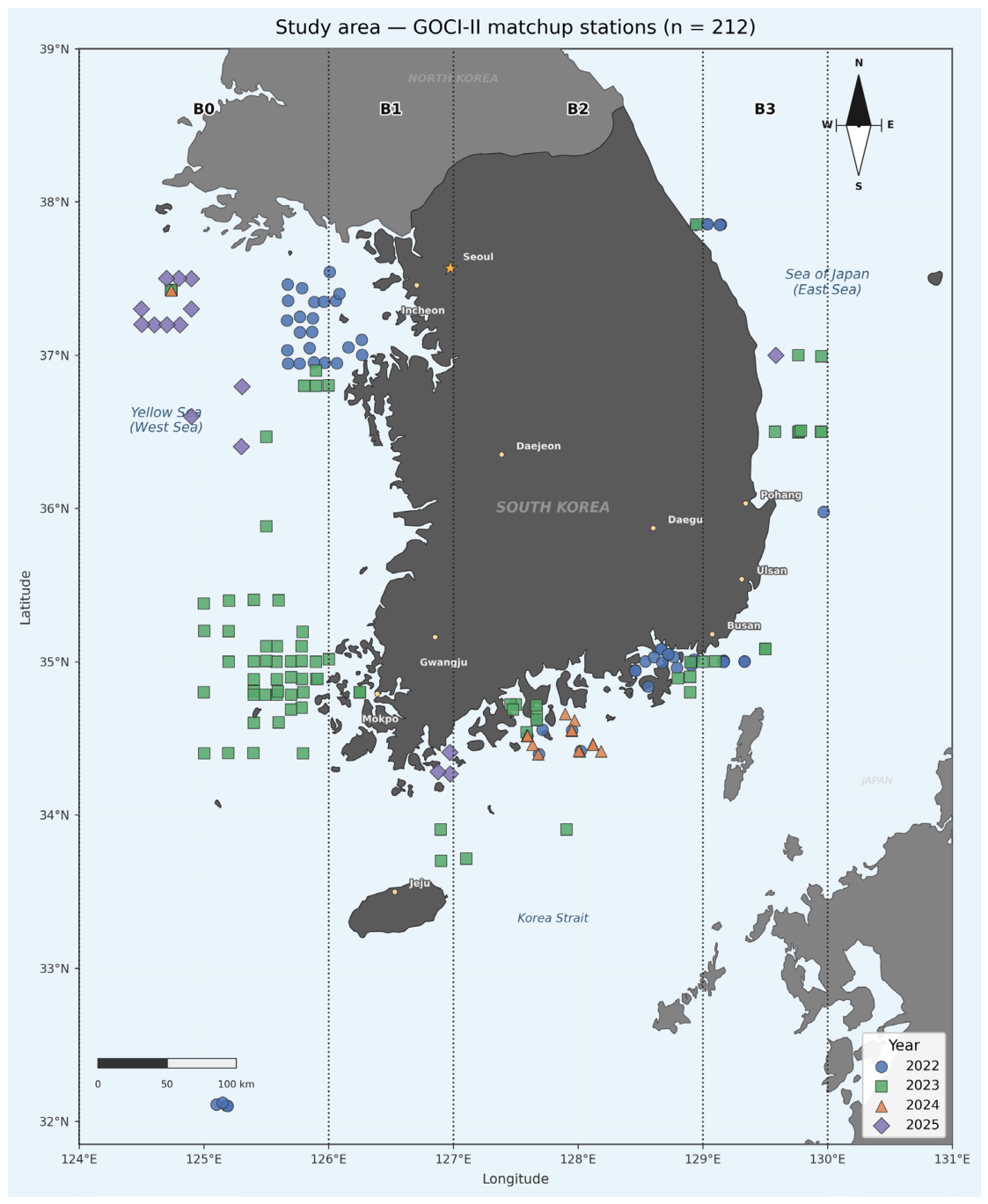
Figure 3.
Spectral characterization: (a) mean ±1 SD Rᵣₛ spectra by turbidity regime; (b) in situ vs. satellite Rᵣₛ scatter at 555, 620, and 709 nm; (c) log-log scatter of Rᵣₛ(620) vs. in situ TSM. The dominant role of the 620 nm channel is consistent with mineral backscattering theory [2,31].
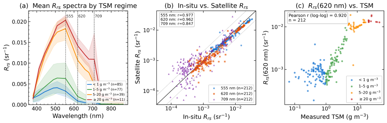
Figure 4.
PISE modeling pipeline. Five physically interpretable spectral features are fed into three base learners: gradient boosting (GB), support vector regression (SVR), and Bayesian ridge (BR). Their out-of-fold predictions are combined by a Ridge meta-learner to produce the final TSM estimate ŷ, which is winsorized at the cap c = 50 g m⁻³ during training.
Figure 4.
PISE modeling pipeline. Five physically interpretable spectral features are fed into three base learners: gradient boosting (GB), support vector regression (SVR), and Bayesian ridge (BR). Their out-of-fold predictions are combined by a Ridge meta-learner to produce the final TSM estimate ŷ, which is winsorized at the cap c = 50 g m⁻³ during training.
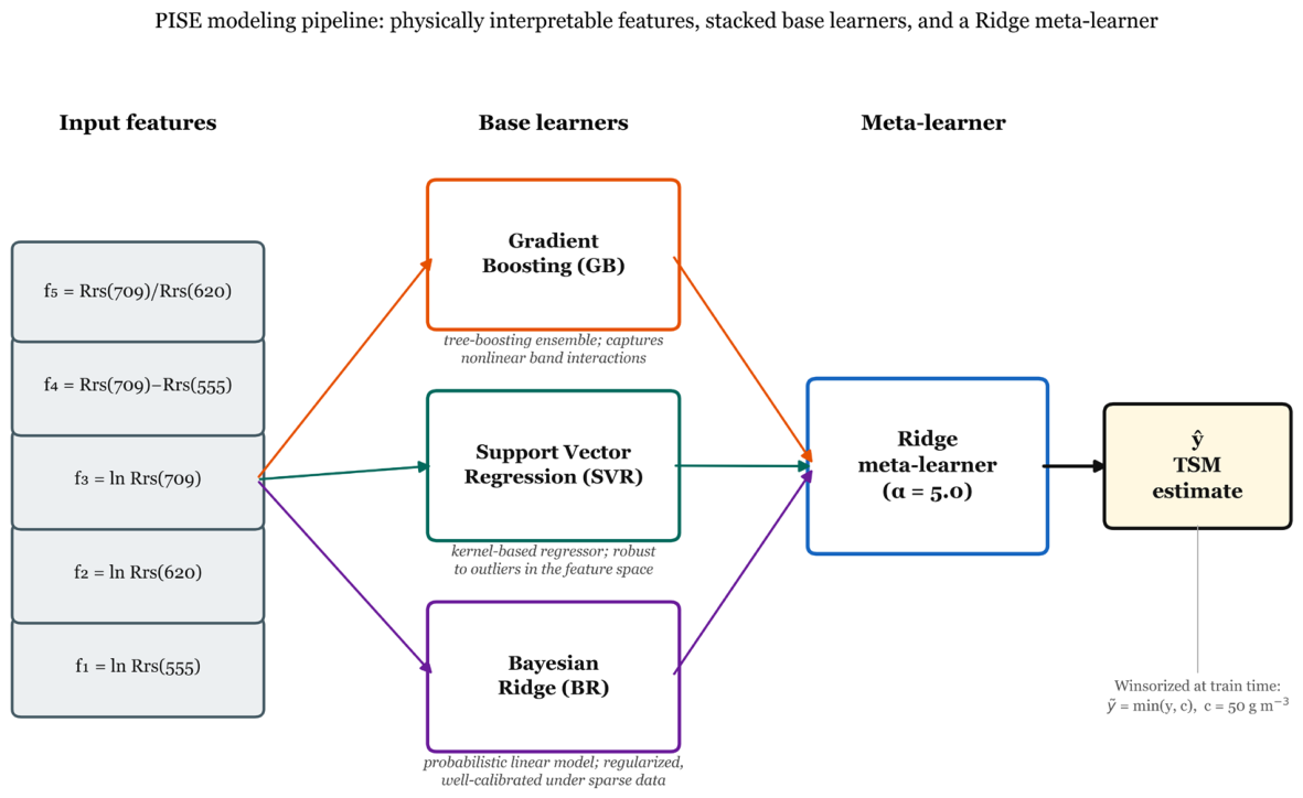
Figure 5.
Scatter plots of PISE (left) and GOCI-II ATBD (right) predicted vs. in situ TSM on the held-out test set (n = 64), colored by collection year. The 1:1 line (dashed) and linear regression fit (solid) are shown. The GOCI-II empirical retrieval ceiling at 28.13 g m⁻³ (dotted) is visible as a hard upper boundary in the right panel.
Figure 5.
Scatter plots of PISE (left) and GOCI-II ATBD (right) predicted vs. in situ TSM on the held-out test set (n = 64), colored by collection year. The 1:1 line (dashed) and linear regression fit (solid) are shown. The GOCI-II empirical retrieval ceiling at 28.13 g m⁻³ (dotted) is visible as a hard upper boundary in the right panel.
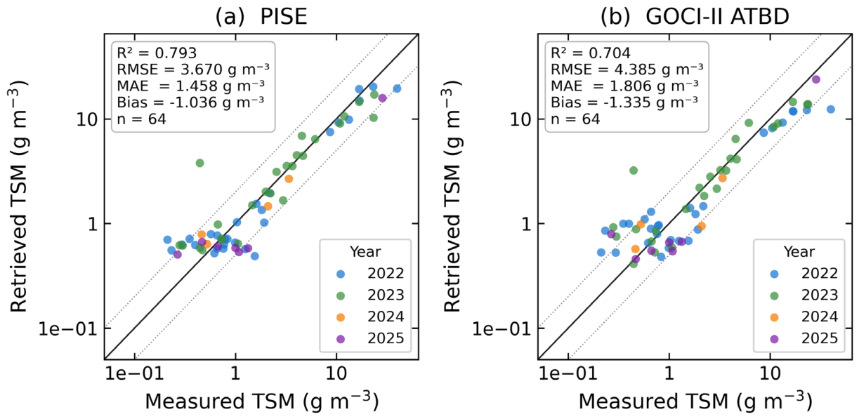
Figure 6.
GOCI-II empirical-ceiling analysis: (a) scatter plot of the predicted vs. in situ TSM, showing the hard ceiling at 28.13 g m⁻³; (b) PISE and GOCI-II RMSE and R² against the winsorization cap value, with the shaded red region indicating the ceiling-exceeding regime (TSM > 28.13 g m⁻³) in which the operational band-ratio formulation's dynamic range is exhausted and the retrieval accuracy cannot improve regardless of the cap; (c) regime-bar chart of R² and (d) RMSE for TSM > 20, > 28 (GOCI ceiling), and > 30 g m⁻³. Both models produce negative R² values above 20 g m⁻³ because of training data scarcity; GOCI-II retains a marginal RMSE and R² advantage in the broader TSM > 20 g m⁻³ regime, where its power-law algorithm has not yet reached its ceiling for most samples, but PISE achieves both a lower RMSE and a higher R² than GOCI-II in the two regimes that are entirely beyond the operational ceiling (TSM > 28 and TSM > 30 g m⁻³), where GOCI-II is hard-bounded at 27.31 g m⁻³.
Figure 6.
GOCI-II empirical-ceiling analysis: (a) scatter plot of the predicted vs. in situ TSM, showing the hard ceiling at 28.13 g m⁻³; (b) PISE and GOCI-II RMSE and R² against the winsorization cap value, with the shaded red region indicating the ceiling-exceeding regime (TSM > 28.13 g m⁻³) in which the operational band-ratio formulation's dynamic range is exhausted and the retrieval accuracy cannot improve regardless of the cap; (c) regime-bar chart of R² and (d) RMSE for TSM > 20, > 28 (GOCI ceiling), and > 30 g m⁻³. Both models produce negative R² values above 20 g m⁻³ because of training data scarcity; GOCI-II retains a marginal RMSE and R² advantage in the broader TSM > 20 g m⁻³ regime, where its power-law algorithm has not yet reached its ceiling for most samples, but PISE achieves both a lower RMSE and a higher R² than GOCI-II in the two regimes that are entirely beyond the operational ceiling (TSM > 28 and TSM > 30 g m⁻³), where GOCI-II is hard-bounded at 27.31 g m⁻³.
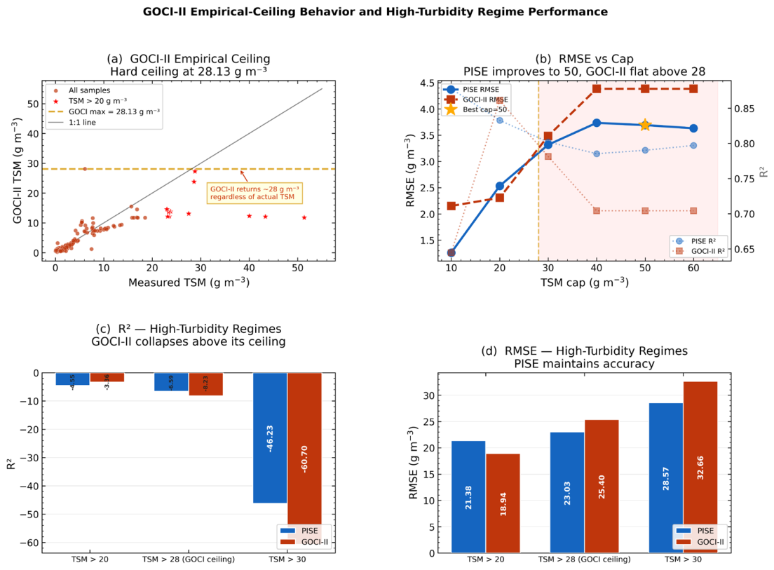
Figure 7.
Model comparison, ablation, and overfitting diagnostics on the held-out test set. Base learner ablation: (a) R², (b) RMSE, and (c) MAE for each base learner (GB, SVR, BR alone), PISE (stacking), and the operational GOCI-II ATBD. Overfitting and cross-validation stability: (d) train vs. test R² for each base learner and PISE, with the generalization gap Δ annotated above each pair; (e) gradient boosting (GB) learning curve, showing the train/cross-validation gap that motivates the stacking ensemble; (f) 5-fold cross-validation stability of GB vs. PISE, showing that PISE achieves a lower fold-to-fold standard deviation.
Figure 7.
Model comparison, ablation, and overfitting diagnostics on the held-out test set. Base learner ablation: (a) R², (b) RMSE, and (c) MAE for each base learner (GB, SVR, BR alone), PISE (stacking), and the operational GOCI-II ATBD. Overfitting and cross-validation stability: (d) train vs. test R² for each base learner and PISE, with the generalization gap Δ annotated above each pair; (e) gradient boosting (GB) learning curve, showing the train/cross-validation gap that motivates the stacking ensemble; (f) 5-fold cross-validation stability of GB vs. PISE, showing that PISE achieves a lower fold-to-fold standard deviation.
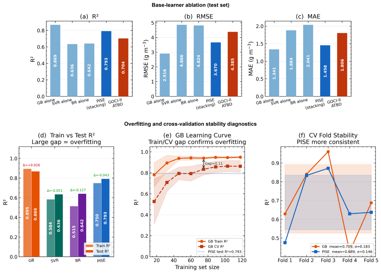
Figure 8.
Uncertainty quantification: (a) predicted vs. in situ TSM with 90% conformal prediction intervals [32,33] achieving q̂ = 3.04 g m⁻³ and 90.6% empirical coverage; (b) permutation sanity check [34] under 1000 random feature permutations (maximum R²: 0.004; threshold 0.10, dashed); (c) Taylor diagram comparing PISE, GOCI-II, and base learners.
Figure 8.
Uncertainty quantification: (a) predicted vs. in situ TSM with 90% conformal prediction intervals [32,33] achieving q̂ = 3.04 g m⁻³ and 90.6% empirical coverage; (b) permutation sanity check [34] under 1000 random feature permutations (maximum R²: 0.004; threshold 0.10, dashed); (c) Taylor diagram comparing PISE, GOCI-II, and base learners.
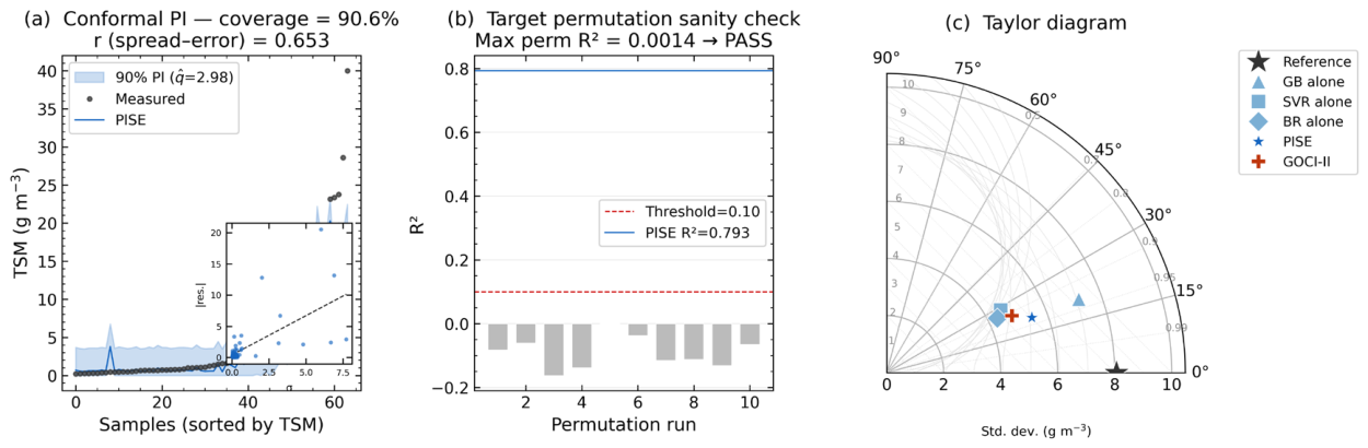
Figure 9.
Spatial PISE TSM fields at contrasting tidal phases for 4 May 2025 (KST) with 24-hour tidal curves at three KHOA stations (Gyeonggi, Mokpo, Jeju). (a) Flood phase (10:15 KST; Gyeonggi Bay tidal height 724 cm): PISE TSM with GOCI-II surface current vectors color-coded by speed (RdYlBu_r); tidal height annotations and wind speed (m s⁻¹) for each ROI station are shown in the inset boxes. (b) Ebb phase (14:15 KST; Gyeonggi Bay tidal height 422 cm): same layout as in Panel (a). Bottom panel: 24-hour tidal height curves at the Gyeonggi (purple), Mokpo (red), and Jeju (blue) stations from the KHOA; stars indicate scenes; filled triangles indicate all ten GOCI-II observation times (red = flood, blue = ebb). SSC = sea surface current. The 302 cm difference in tidal height between the two scenes reflects the macrotidal forcing range of the Yellow Sea system [37]. A persistent turbid plume at the Mokpo Coast is present during both tidal phases, confirming the tidal independence of the high-turbidity core [7,22].
Figure 9.
Spatial PISE TSM fields at contrasting tidal phases for 4 May 2025 (KST) with 24-hour tidal curves at three KHOA stations (Gyeonggi, Mokpo, Jeju). (a) Flood phase (10:15 KST; Gyeonggi Bay tidal height 724 cm): PISE TSM with GOCI-II surface current vectors color-coded by speed (RdYlBu_r); tidal height annotations and wind speed (m s⁻¹) for each ROI station are shown in the inset boxes. (b) Ebb phase (14:15 KST; Gyeonggi Bay tidal height 422 cm): same layout as in Panel (a). Bottom panel: 24-hour tidal height curves at the Gyeonggi (purple), Mokpo (red), and Jeju (blue) stations from the KHOA; stars indicate scenes; filled triangles indicate all ten GOCI-II observation times (red = flood, blue = ebb). SSC = sea surface current. The 302 cm difference in tidal height between the two scenes reflects the macrotidal forcing range of the Yellow Sea system [37]. A persistent turbid plume at the Mokpo Coast is present during both tidal phases, confirming the tidal independence of the high-turbidity core [7,22].
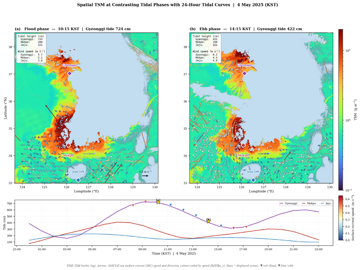
Figure 10.
Integrated diurnal TSM monitoring (4 May 2025): (a) Gyeonggi Bay tidal height (KHOA station) with ten GOCI-II observation times indicated; (b) ROI-mean PISE TSM at Gyeonggi Bay (blue), Mokpo Coast (red), and Jeju Offshore (green) across all ten scenes; (c) ROI-mean TSM vs. Gyeonggi Bay tidal-stage gauge reading with linear regression fits (Gyeonggi: +0.006, Mokpo: +0.003, Jeju: +0.017 g m⁻³ cm⁻¹; [57]; (d) Hovmöller diagram of PISE TSM along the western Korean coastal transect (126.0°E, 36.5–37.8°N). The flood-ebb bar beneath Panels (a) and (d) indicates the tidal phase following Fang et al. [37].
Figure 10.
Integrated diurnal TSM monitoring (4 May 2025): (a) Gyeonggi Bay tidal height (KHOA station) with ten GOCI-II observation times indicated; (b) ROI-mean PISE TSM at Gyeonggi Bay (blue), Mokpo Coast (red), and Jeju Offshore (green) across all ten scenes; (c) ROI-mean TSM vs. Gyeonggi Bay tidal-stage gauge reading with linear regression fits (Gyeonggi: +0.006, Mokpo: +0.003, Jeju: +0.017 g m⁻³ cm⁻¹; [57]; (d) Hovmöller diagram of PISE TSM along the western Korean coastal transect (126.0°E, 36.5–37.8°N). The flood-ebb bar beneath Panels (a) and (d) indicates the tidal phase following Fang et al. [37].
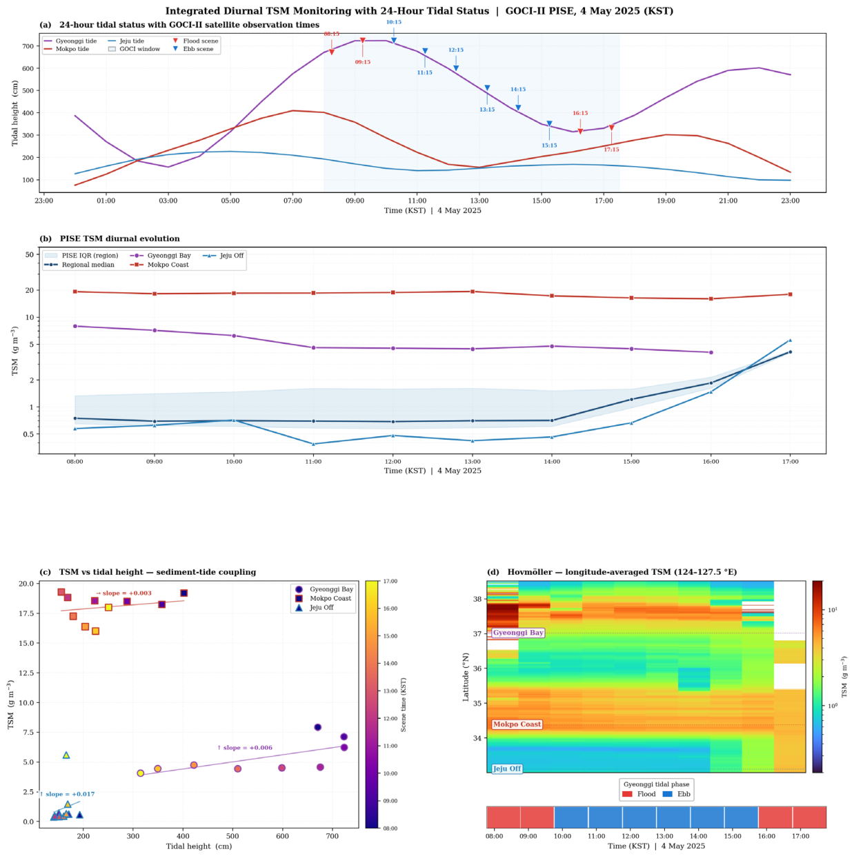
Table 2.
Overall performance on the held-out test set (n = 64). Bold values indicate better performance per metric. R² confidence interval from 1000 bootstrap resamples. Units of the RMSE, MAE, and bias are g m⁻³.
Table 2.
Overall performance on the held-out test set (n = 64). Bold values indicate better performance per metric. R² confidence interval from 1000 bootstrap resamples. Units of the RMSE, MAE, and bias are g m⁻³.
| Model | R² (95 % CI) | RMSE | MAE | Bias | SMAPE (%) | LogRMSE |
| PISE | 0.793 (0.715, 0.934) | 3.670 | 1.458 | −1.036 | 35.65 | 0.228 |
| GOCI-II ATBD | 0.704 | 4.385 | 1.806 | −1.335 | 43.25 | 0.258 |
Table 3.
Cap sensitivity analysis: PISE and GOCI-II ATBD performance across six winsorization caps. The asterisk indicates the selected cap. Bold: optimal PISE entry. Units of the RMSE are g m⁻³.
Table 3.
Cap sensitivity analysis: PISE and GOCI-II ATBD performance across six winsorization caps. The asterisk indicates the selected cap. Bold: optimal PISE entry. Units of the RMSE are g m⁻³.
| Cap (g m⁻³) | n within cap | PISE R² | PISE RMSE | GOCI-II R² | GOCI-II RMSE |
| 10 | 186 | 0.879 | 1.256 | 0.645 | 2.151 |
| 20 | 201 | 0.826 | 2.584 | 0.861 | 2.309 |
| 30 | 209 | 0.804 | 3.304 | 0.781 | 3.485 |
| 40 | 210 | 0.779 | 3.788 | 0.704 | 4.385 |
| 50* | 211 | 0.793 | 3.670 | 0.704 | 4.385 |
| 60 | 212 | 0.781 | 3.771 | 0.704 | 4.385 |
Disclaimer/Publisher’s Note: The statements, opinions and data contained in all publications are solely those of the individual author(s) and contributor(s) and not of MDPI and/or the editor(s). MDPI and/or the editor(s) disclaim responsibility for any injury to people or property resulting from any ideas, methods, instructions or products referred to in the content. |
© 2026 by the authors. Licensee MDPI, Basel, Switzerland. This article is an open access article distributed under the terms and conditions of the Creative Commons Attribution (CC BY) license (http://creativecommons.org/licenses/by/4.0/).
Copyright: This open access article is published under a Creative Commons CC BY 4.0 license, which permit the free download, distribution, and reuse, provided that the author and preprint are cited in any reuse.