

Submitted:
23 September 2026
Posted:
24 September 2026
You are already at the latest version
Abstract
Common intuitions suggest that the largest available model is always best, but what about when one LLM predicts or stands in for another? We present scale affinity: the observation that models of a similar size are often best at matching another model’s behavior, meaning bigger is not always better. We first establish this distributionally: testing the ability to predict LLM generations across up to 23 models in 5 data domains, we find the best predictor of a given model’s text is most often a similarly-sized model within the same family, and the trend against pure scale holds across family boundaries. The effect is not an artifact of likelihood-based measurement: similarly-sized models also reproduce each other’s errors on multiple-choice benchmarks beyond what matched accuracy explains, and smaller in-family models are better adversarial predictors of another model’s moves. Scale can eventually help with behavior matching, but typically only at much larger sizes and with more observed context than similarly-sized models require, suggesting that scale affinity and scaling laws (bigger is better) are opposing factors that trade off to determine how effectively one LLM can predict another. Scale affinity has significant implications when using models to stand in for other systems, suggesting that matching capability to the target can be a better choice than simply using the strongest LLM available.
Keywords:
LLM
; simulation
; prediction
; natural language generation
1. Introduction
LLMs are increasingly asked to stand in for other models: a red-team model probes for another model’s failures (Perez et al. 2022), an adversarial model must anticipate what a target model will do, and a draft model must anticipate a target model’s tokens. In every such setting, a practitioner faces the same selection question—which model best predicts the behavior of another?—and the common default is to reach for the largest model available. This default reflects the scaling laws that have driven recent LLM development: larger models achieve lower perplexity, capture more nuanced patterns, and outperform their smaller counterparts on almost every benchmark (Kaplan et al. 2020,Hoffmann et al. 2022). Given a blackbox 7B parameter LLM, it therefore seems likely that a 70B model would predict its generations better than another 7B model. Counter to this intuition, we introduce scale affinity, the observation that when it comes to predicting another model’s behavior, similarity of model size can matter more than the absolute size of the predictor alone—in other words, 7B LLMs may be best at matching each other.
We focus on a principled formulation inspired by pretraining itself: document continuation. Given a document written by a target LLM, how accurately can a predictor complete it as context grows? We can use cross-entropy (CE) over model generated documents here to test how well a predictor model can match a target model’s distribution.
Figure 1.
Scale affinity is the tendency of LLMs of similar size, rather than simply the largest, to achieve the lowest loss on generations from other models. Here, OPT 350m is used to generate with many other models competing to match its distribution in-context.
Figure 1.
Scale affinity is the tendency of LLMs of similar size, rather than simply the largest, to achieve the lowest loss on generations from other models. Here, OPT 350m is used to generate with many other models competing to match its distribution in-context.
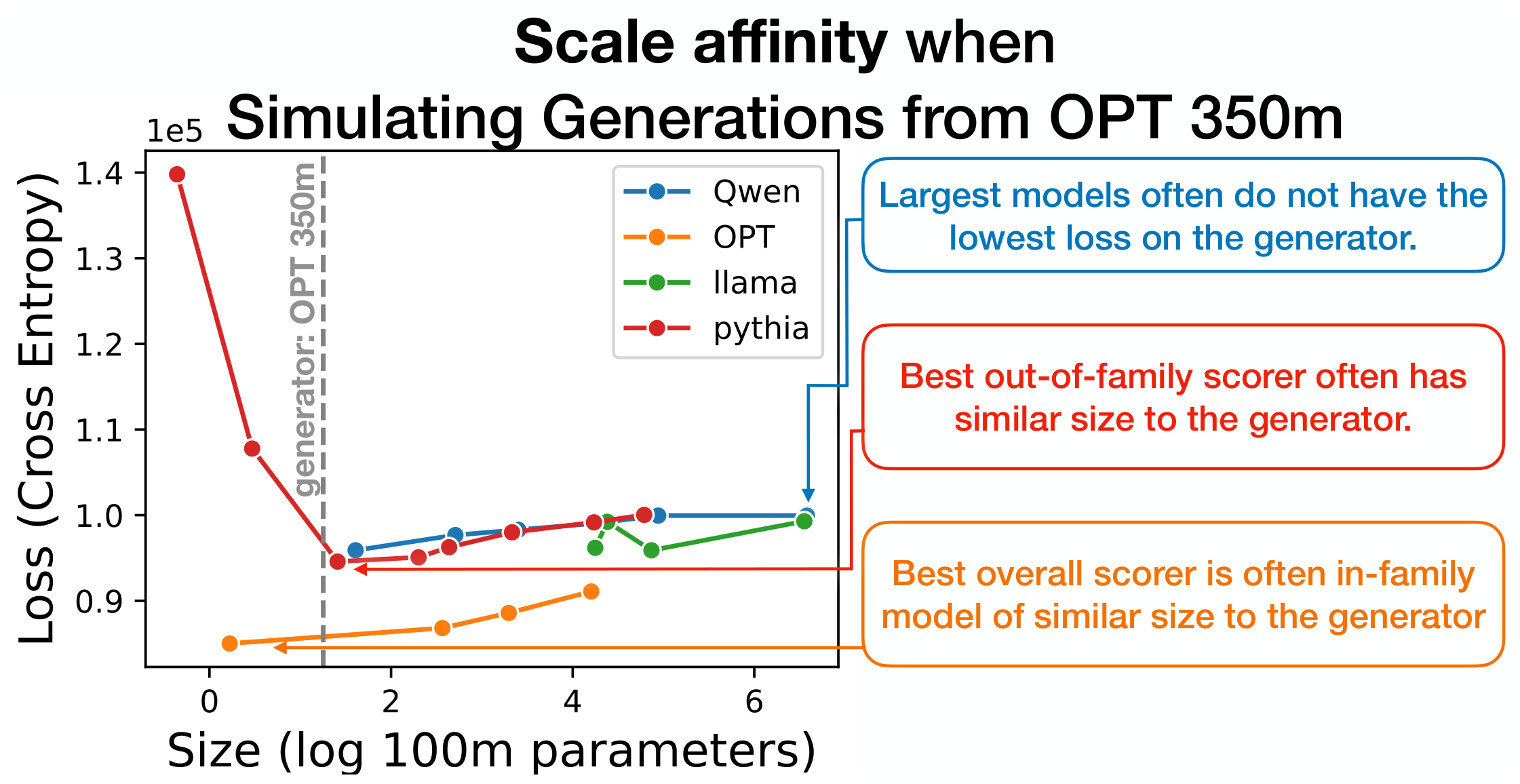
Our experiments broadly support the notion that large scale alone is not the best recipe for predicting another model’s generations, and scale affinity—similar size—is often a more important factor in our setting. We test up to 23 models from 4 families across 5 text domains. In each experiment, one target model generates many documents based on domain-specific human prefixes, and we use CE loss across all other models to identify the best predictor (in-family and out-of-family). We find a large number of cases where the best predictor is a model of similar size to the target, rather than simply the largest available model. While the winner between the largest model and the one most similar in size depends on domain and setting, scale alone is clearly not always the winning recipe.
Because cross-entropy is a distributional measure, a natural concern is that scale affinity is an artifact of likelihood-based scoring rather than a property of how models behave. We therefore test the same question with two task-level measures that involve no log-probabilities: whether models reproduce each other’s errors on multiple-choice benchmarks, and whether smaller models are better adversarial predictors of another model’s moves in a repeated game. Both recover the affinity pattern, indicating that similarly-sized models do not merely assign similar probabilities—they fail in the same way, and are easier for scale-matched adversaries to anticipate.
Analysis suggests why similar-sized models win: an example-level view (Table 1) points to larger models being unable to reproduce the mistakes of small ones—for example, in finding the greatest common factor of two integers. Larger models are more likely to win given longer generated context, or when the size gap is especially large.
This gives a concrete setting in which scaling laws are not the dominant factor in success, relevant to adversarial attack, red teaming, and replacing closed models a user cannot access. While we focus on LLMs predicting LLMs, the question generalizes: as LLMs stand in for other systems, including humans, it matters whether to reach for the most capable model or one matched to the target—and in the latter case, much more work is needed on training for similarity rather than absolute strength.
2. Scale Affinity
Many use cases have LLMs stand in for other systems—coders, customer service agents, even simulated societies (Park et al. 2023). A directed version: what should we use to predict the behavior of another LLM we lack access to? The scaling philosophy says bigger is always better (Kaplan et al. 2020,Henighan et al. 2020)—use the largest model available, regardless of task. But models of different sizes have fundamentally different qualities, as work on scaling laws (Henighan et al. 2020), emergent abilities (Wei et al. 2022), and U-shaped scaling (McKenzie et al. 2024) suggests. A model of similar size and strength may therefore be a natural analog, and the best predictor. We call this scale affinity. One intuition: small LLMs make very different mistakes than large ones. A large LLM may have learned to avoid an error entirely—useful in general, but it makes reproducing a smaller model’s errors unnatural. As Oh and Linzen (2025) note, frontier LLMs are now too strong along some axes to model even human attributes.
One basic intuition that supports this idea is that smaller LLMs produce very different generations than large ones, and especially make very different mistakes. A very large LLM may have learned to avoid a certain error, which is useful in general, but would make reproducing those errors of the smaller model unnatural. As Oh and Linzen (2025) note, frontier LLMs are now too strong along certain axes to model even some human attributes.
In this work, we first study scale affinity as it relates to predicting model generations in-context. Simply, which model S can best approximate the output of target model G in a given context? This can be directly measured using the same cross-entropy loss used by LLMs to match the underlying distribution of human text (Figure 2). We limit our study to already-trained models, testing prediction as an existing capability. In essence, can a given model match a distribution that it is dropped into?
Why cross-entropy, and why pure sampling.
Cross-entropy is not merely a proxy for distributional similarity here; under our setup it is a direct measure of it. When text is sampled from generator G at temperature with no truncation, the expected loss a scorer S assigns to G’s samples is the cross-entropy , which decomposes exactly as
The first term, the generator’s own entropy, depends only on G: when we hold the generator fixed and compare scorers, it is a constant added equally to every scorer and cannot change their ranking. The entire ordering of scorers is therefore decided by the second term—the forward KL divergence from the generator to the scorer. Asking “which model best predicts G’s outputs” is, at the population level, exactly asking “which model’s distribution is closest in KL to G’s.” This decomposition also fixes our decoding choice: with pure ancestral sampling is not a tunable hyperparameter but the unique setting under which the sampled text genuinely comes from G’s distribution—any other temperature would measure closeness to a sharpened or flattened distortion of G instead. Finally, it disposes of a potential entropy confound: a higher-entropy generator raises , lifting every scorer’s loss by the same constant while leaving the ranking untouched. We verify this empirically with a symmetric temperature sweep in which the scorer ranking is unchanged across , up to a single statistical tie between two scorers at (paired ; the technical supplement). Because this argument is specific to distribution matching, we complement the cross-entropy experiments with task-level measures of behavior matching that involve no log-probabilities.
3. Experiments
3.1. Experimental Setup
Task.
A single generator model , the target, produces continuations of a set of contexts, and scorer models of varying sizes score those continuations under their own distributions. Some scorers share the generator’s family; others do not.
Generation.
Let denote a context of tokens drawn from a corpus. For each context, we sample a continuation of tokens from the generator:
where denotes the sequence of generated tokens.
Scoring.
Each scorer model then evaluates the generator’s continuation by computing the log-probability it assigns to the sampled tokens conditioned on the same context:
This measures how well accounts for the token-level choices of . Because we use pure sampling, it corresponds directly to the divergence between the two distributions. A strong predictor conforms quickly to the generator’s distribution. We note that no scorer can achieve a lower expected loss on ’s generations than itself: in expectation the generator’s own loss is its entropy , the minimum of the cross-entropy in Equation 1, attained only when the scorer’s distribution equals the generator’s. Scorers are therefore competing to come as close as possible to this lower bound, and we exclude the generator from the set of scorers throughout.
Varying in Equation 3 lets the scorer condition on generated tokens before scoring: scores the whole generation, while e.g. with treats the first 50 generated tokens as context and scores the next 50.
Experimental setting.
Our primary experiment takes -token contexts from 500 Pile documents (Gao et al. 2020); generators produce tokens, which scorers then score. Extended settings generate up to tokens and score a later subsequence, giving scorers generated context to learn from.
Data and Models.
We evaluate 23 models spanning 4 families: Pythia (70M, 160M, 410M, 1B, 1.4B, 2.8B, 6.9B, 12B) (Biderman et al. 2023), OPT (125M, 350M, 1.3B, 2.7B, 6.7B) (Zhang et al. 2022), Qwen 2.5 (0.5B, 1.5B, 3B, 7B, 14B, 72B) (Team 2024), and Llama, including Llama 2 (7B, 13B) (Touvron et al. 2023) and Llama 3.1 (8B, 70B) (Grattafiori et al. 2024). Models range from 70M to 72B parameters; all core cross-entropy experiments use base (pretrained, non-instruction-tuned) models, while the task-level experiments on multiple choice and adversarial games state their base/instruct choices individually. The two largest models (Qwen 2.5-72B and Llama 3.1-70B) are loaded in 4-bit quantization via bitsandbytes (Dettmers et al. 2022) due to memory constraints (NF4 with double quantization and bfloat16 compute dtype); all others run in bfloat16 precision. We note that this confound runs against the large models rather than in their favour: quantization flattens a model’s output distribution, and a flatter distribution sits closer in KL to the distribution it is asked to reproduce, which is precisely what our metric rewards. Quantized large models also remain stronger than smaller full-precision models on conventional benchmarks (Dettmers and Zettlemoyer 2023). A controlled bfloat16-versus-NF4 comparison remains future work, and effect sizes may shift, but the direction of the bias does not explain large models losing. Note: for the purposes of plotting scale, we follow Kaplan et al. (2020) in using log(# parameters), specifically using 100m parameters as the base unit (see Figure 1 for example). We note that parameter size is not always indicative of general model capabilities or test loss, but focus on scale rather than other measures such as perplexity on human data as we are specifically contrasting with scaling laws. Future studies should investigate other measures of model strength besides scale.
We evaluate on five text domains: (1) The Pile (Gao et al. 2020), a mixed-domain corpus spanning web text, books, academic papers, and code; (2) WikiText-103 (Merity et al. 2017), encyclopedia text; (3) ArXiv scientific papers (Cohan et al. 2018); (4) Python code from CodeSearchNet (Husain et al. 2019); and (5) CNN/DailyMail news articles (See et al. 2017). Experiments on domains besides the Pile use 500 prefixes and up to 400 generated tokens with 21 models (excluding the two largest due to computational constraints). Note that the majority of our experiments focus on the most general of these domains: the Pile.
Tokenization.
Tokenization varies across families, so we treat the generator’s tokenization as canonical: each scorer reports the log-probability, under its own tokenization, of the text spanned by the generator’s first tokens. Scores are therefore comparable across scorers for a fixed generator, though not across generators. We sum log-probabilities over the scored span, avoiding length-normalization issues.
3.2. Results and Discussion
Scale affinity.
The primary results for scale affinity are presented in Figure 3: plotting the (log) sizes of the generating model and best scoring model for each experiment. Under a classic scaling laws assumption that larger scale is always better, we would expect the best scorer to be the largest model, regardless of generator size, i.e., all points would be along the top axis (in the orange band marked scaling laws).
In our main experiment on the Pile corpus (left), we see relatively little support for the power of scale in this experiment. For both in-family and out-of-family models, each best scorer tends to be quite similar in size to the generating model. In other words, the model that is best at matching the distribution of a given generator tends to be a model of a similar size rather than the largest available model in these experiments. This strongly supports the notion of scale affinity. Of particular note is the fact that this holds for out-of-family scoring models. This suggests that scale affinity is not simply a function of the specific training recipe, but rather a fundamental similarity between general LLMs of a similar size and strength which crosses model family boundaries.
Statistical robustness of the best scorer.
Because reporting only the argmin scorer discards information about margins and uncertainty, we quantify the reliability of each reported best scorer with a bootstrap over the 500 prefixes (2,000 resamples per generator–domain cell, self-scoring excluded; 107 cells total across the five domains). The identity of the best scorer is highly stable: the same scorer is the argmin in of bootstrap resamples on average (median ). The margin between the best and second-best scorer is itself significant—its bootstrap confidence interval excludes zero—in of cells. Across all cells, the best scorer lies within orders of magnitude of the generator’s size in of cases, belongs to the generator’s own family in , satisfies both—a similarly-sized model within the same family—in , and is the largest available model in only . Beyond the argmin, the full ranking is consistent with affinity: the Spearman correlation between a scorer’s mean loss and its absolute log-size gap to the generator is positive on average (), meaning scorers further from the generator in scale tend to score worse throughout the ranking, not merely at the top. Per-cell values are given in the technical supplement.
Predicting very small models.
One notable exception appears in Figure 3 (left): for the smallest generator (Pythia 70m), the best out-of-family scorer is very large rather than similarly sized. Loss curves for the four smallest generators (the technical supplement) show this is not a fluke—a local minimum near the generator’s scale, then a rise, then an eventual drop at much larger scale. The best scorer (Llama 3.1 70B) is roughly the generator’s size, and the only large model to beat the most scale-similar one (OPT 125m). This suggests a tension between scale affinity and scaling laws: with a large enough gap, strength can beat similarity. We caution against over-reading a single case—Pythia 70m is the weakest model we test and its generations are unusually high-entropy, so a strong LM may model them well simply because they approach easy-to-cover noise. The non-monotonic shape recurs in our error-agreement analysis under an independent task-level metric, so the local minimum does not hinge on this point.
Effect of generated context.
Longer generations benefit scale: varying generated tokens from to 200 (the technical supplement), cases where a very large model is the best predictor grow from 2 to 7, consistent with large scorers learning about the generator in context. The benefit accrues mainly to large scorers on small generators and to out-of-family scorers; in-family scorers are less affected and continue to follow scale affinity. Giving scorers generated context before the scored span (0–150 tokens preceding 50 scored tokens; the technical supplement) flips the shape of the out-of-family curve, again increasing the value of scale, while in-family curves keep their shape—scale affinity persists even with substantial context.
Effect of domain.
Figure 3 (right) plots log size of each generator model against its most effective scorer, on domains besides the Pile. This includes arXiv, code, news, and wiki text. Note that we do not include the 2 largest models in these experiments due to computational limitations, which changes the max log size in these plots.
Unlike results on the Pile, we see a mix of preference for absolute (large) scale, and scale affinity. For example, in our experiment on arXiv data, the best (in-family) scorer is in many cases the largest model in the family, even for relatively small generators. Broadly, this supports the notion that scale affinity is in tension with the value of larger scale when it comes to prediction—depending on the domain and experimental setting, the best scorer may be the result of one effect or the other.
While the best in-family model was often the largest for arXiv, the best out-of-family scorers more often followed scale affinity. We see exactly the opposite for the code domain, where the best out-of-family scorers were often the largest of a complementary family (for example, Llama 13B was often the best scorer for OPT models). The exact reason for this likely depends on specific attributes of each domain. One key difference in this case is that generating models had a much higher self-entropy in the arXiv domain than the code domain—a median of against nats/token over the same generators, a factor of . This may indicate less specific decisions made by the model, as it is closer to uniform random sampling, which could be easy for larger models to recognize and predict.
Token-level analysis.
Finally, we ask on which tokens similarly-sized models out-compete larger ones. Using one family (Qwen) so tokenization is consistent, with Qwen 2.5 0.5B as generator—a setting where the smaller scorer wins—we compare the largest scorer (Qwen 2.5 72B) against the closest in size (Qwen 2.5 1.5B) in the technical supplement. Most tokenwise mass lies above the line, as expected, with a few large outliers. Bucketing the summed loss difference by gap size shows the small model’s advantage comes mostly from many tokens with modest differences rather than a few outliers—a slight but consistent edge.
We present a few examples with some of the largest token-wise loss differences in Table 1, to gain intuition for why a similarly-sized model can be a better predictor. In this table, indicates the difference between the loss of model m on the given token, and the loss of the generator (optimal in expectation). We compare the same large and small model as above. The first example is particularly informative: the context asks for the greatest common factor between 18 and 6024. Both the generator and the small scorer give low loss to the generated token (“1”, at the beginning of “18”), as indicated by low . The large model gives much higher loss to this token, which makes sense given that the greatest common factor is actually “6”. In this case, the larger model knows the correct answer to the given question, which actually makes it harder to predict a smaller generator that does not. Scale affinity may be partially explained by smaller models making similarmistakes.
4. Scale Affinity Beyond Log-Likelihood
The cross-entropy results establish scale affinity as a distributional property. A distinct question is whether the pattern carries into how models behave: which answers they produce, and whether their moves can be anticipated. In this section, we test this with two measures that involve no log-probabilities, extending our core results. Both settings support scale affinity.
4.1. Do Similarly-Sized Models Make the Same Mistakes?
If scale affinity reflects genuine behavioral similarity, similarly-sized models should not merely fail at the same rate—they should fail in the same way. We measure how often one model reproduces another’s incorrect multiple-choice answers across 22 models on ARC-Challenge (1,172 items) (Clark et al. 2018) and a 3,000-item MMLU subset (Hendrycks et al. 2021).
A similarly-sized, same-family scorer reproduces a target’s errors significantly more often than the largest model does: bootstrapping over items, the gap between the best in-family scorer and the largest model has a confidence interval excluding zero for 21 of 22 targets on ARC and 20 of 22 on MMLU, with median gaps of and . Within-family error reproduction averages on ARC and on MMLU, against and for the largest model (Qwen2.5-72B). The cross-family version of the claim is weaker and we state it as such: the best in-family scorer beats the best cross-family scorer with a CI excluding zero for 18 of 22 targets on ARC and 19 of 22 on MMLU, and the gap is slightly negative for Qwen2.5-0.5B and Llama-3.1-8B. Because raw capability is a known independent driver of shared errors across models (Goel et al. 2025,Kim et al. 2025), we regress pairwise error agreement on the absolute accuracy gap, same-family membership, and log-size gap ( pairs, ): we want the part of error-sharing that scale and family explain beyond mere equal accuracy. After this control, both same-family (, ) and similar scale ( per unit log-size gap, ) independently predict shared errors. Two models of similar size fail in the same way, not merely at the same rate—consistent with the finding that, controlling for other factors, models closer in size have more correlated errors (Kim et al. 2025). Notably, this result also bears on the hypotheses of our discussion (below): the most capable model is the worst at reproducing a mid-sized model’s errors, the opposite of what pure capability maximization would predict.
4.2. Can a Scale-Matched Adversary Better Anticipate a Model’S Moves?
Finally, we test the active end of behavior prediction, where anticipating another model is the explicit objective: in repeated rock-paper-scissors, an adversarial “predictor” sees a player model’s move history, predicts its next move, and counters. We run 7 players against 5 predictors (Llama-3.1 8B/70B; Qwen3 8B/14B/32B), 20 games of 10 rounds each, all instruct models.
The smallest model within a predictor family is the most effective adversary for 6 of 7 players; in the single case where the largest model in a family beat all smaller ones (Qwen3-32B predicting Llama-3.2-3B), it still lost to the much smaller Llama-3.1-8B predictor. While this is a toy setting, it shows better prediction translating into utility—“winning”—and, because the objective is move prediction rather than likelihood, the effect again holds outside log-probability matching entirely.
Passive and active prediction.
Our core cross-entropy experiments never instruct any model to imitate another; they measure whether affinity emerges naturally from how models score one another’s text. This passive regime is the one relevant to red-teaming and stand-in evaluation, where a model is never told to “act like a 7B model.” Whether a large model can be explicitly prompted or tuned into a better imitator is a distinct, open question: prior work shows large models can be steered toward weaker behavior when instructed, though imperfectly (Gudibande et al. 2024). The adversarial game probes the opposite, explicitly-rewarded end—and the largest model still does not dominate. Passive and active settings converge on the same conclusion: scale alone does not determine how well one model predicts another.
5. Discussion
5.1. Why Does Scale Affinity Occur?
We consider two complementary hypotheses for the origin of scale affinity.
Hypothesis 1: Capability matching.
A model’s generated text reflects its capability level—vocabulary diversity, syntactic complexity, factual consistency, stylistic preference. A similarly-capable scorer shares these biases and assigns lower surprise to text resembling what it would have generated. Similar-scale models are known to achieve similar overall loss, but that need not imply similar distributions, only equal inability to capture the training distribution; if this hypothesis holds, similar-quality models genuinely do produce similar distributions—a developmental marking of LLMs. The cross-family results support it: even across different training data and architectures, similarly-sized models are better scorers than much larger or smaller ones, so capability matching operates above training-data overlap.
Hypothesis 2: No true out-of-family models.
Alternatively, overlapping training corpora and near-identical architectures may mean no model is truly out-of-family, and affinity simply reflects similar training dynamics at similar scale. This likely plays some part—a model of wholly different architecture trained on an unfamiliar language would share little with current LLMs. But our results (Figure 3) show markedly different behavior for in-family versus out-of-family scorers, so shared training dynamics cannot be the whole story.
We emphasize that our observational design cannot fully separate these hypotheses: all tested models are autoregressive transformers trained on overlapping web corpora, so “out-of-family” remains a narrow intervention. A clean separation would be interventional—for example, fine-tuning a large model to imitate a small one and testing whether matched capability alone recovers the effect—which we leave to future work. The strongest distinguishing evidence currently available is the error-agreement analysis on multiple choice questions (family and scale each predict shared errors after controlling for the accuracy gap, and the most capable model is the worst at reproducing a mid-sized model’s errors—the opposite of what pure capability maximization would predict. We therefore treat both hypotheses as partially supported.
5.2. Implications
Scale affinity has direct consequences for any setting in which one model is used as a proxy for another. Crucially, these implications no longer rest on cross-entropy alone: the task-level results show the affinity pattern in which answers models produce on multiple-choice questions and in how well an adversary anticipates moves. For red-teaming and adversarial probing—predicting what another model will do—the error-agreement and adversarial-game results apply directly: a scale-matched model reproduces a target’s failure modes and anticipates its moves better than the largest available model, suggesting that matching scale can matter more than maximizing it.
What we do not claim.
Our evidence concerns prediction of another model’s behavior, not evaluation of its quality. LLM-as-judge is a natural place to look for scale affinity, and related work locates judge self-preference in likelihood (Wataoka et al. 2024) and reports that judges favor models similar to themselves (Goel et al. 2025). We ran a pairwise Bradley–Terry judging study, but our generator pool largely lacks the comparisons that would separate scale affinity from a preference for larger, same-family generations, and judges mostly preferred larger generations where that comparison existed. We therefore make no claim about judge preferences, and treat a properly powered judging study as the natural next test.
Standard scaling laws (Kaplan et al. 2020,Hoffmann et al. 2022) characterize loss on held-out natural data as a function of parameter count. Scale affinity reveals structure that this one-dimensional view misses: models at different scales occupy qualitatively different regions of text space, producing outputs most recognizable to models at the same scale—suggesting a multi-dimensional view of model similarity complements the scaling perspective. As LLMs are increasingly used as stand-ins for other systems, including humans and even societies (Park et al. 2023), selecting an effective stand-in matters: building on Oh and Linzen (2025), scale affinity supports the broader notion that a stand-in with capabilities analogous to the target may beat simply maximizing capability and hoping behavior matching follows.
6. Related Work
Scaling laws.
The relationship between model size and performance has been characterized by power-law scaling relationships for self-perplexity (Kaplan et al. 2020,Hoffmann et al. 2022,Henighan et al. 2020). These works study how a model’s perplexity on held-out data decreases with increasing parameter count, data, and compute. However, scaling does not always improve performance: McKenzie et al. (2024) document inverse scaling on multiple tasks where larger models perform worse, and Caballero et al. (2023) show that scaling curves can exhibit non-monotonic transitions that simple power laws fail to capture. Our work reveals a related but distinct phenomenon for cross-model loss: how well model A predicts the output of model B is a non-monotonic function of A’s size, with a minimum often near B’s size rather than at the largest scale.
LLM-as-judge and LLM-as-evaluator.
A growing body of work uses LLMs as evaluators of other models’ outputs (Zheng et al. 2023,Dubois et al. 2024,Gu et al. 2024), standardly using the strongest available model as judge. Recent work reveals systematic biases, including self-preference—favoring outputs with lower perplexity under the judge’s own distribution (Wataoka et al. 2024)—closely related to our cross-perplexity findings. Scale affinity raises the question of whether this assumption deserves further scrutiny—whether a similarly-sized model is better calibrated to the system under evaluation is an open question that our experiments do not settle (Section 5.2).
Model fingerprinting and attribution.
Several works detect which model generated a text from statistical properties of the output (Mitchell et al. 2023,Hans et al. 2024,Bao et al. 2024); Binoculars (Hans et al. 2024) uses cross-perplexity ratios between a model pair directly. Our focus is instead the scaling pattern—how prediction relates to the generator–scorer size relationship—rather than building a classifier.
Simulation of agents and personas.
Recent work uses LLMs to simulate users, populations, or other AI systems (Perez et al. 2022,Park et al. 2023,Shanahan et al. 2023), implicitly assuming a more powerful model is a more faithful simulator. Evidence suggests otherwise: LLM-simulated users are miscalibrated proxies for humans (Seshadri et al. 2026), and current LLMs may be too “super-human” to stand in for human linguistic attributes (Oh and Linzen 2025). Scale affinity offers a complementary perspective, suggesting that selecting a model with similar capabilities to the target system may yield more accurate simulation than simply maximizing the simulator’s size.
7. Conclusions
We introduced scale affinity, the observation that similarly-sized language models are often better at matching each other’s behavior than larger models are at matching smaller ones. Through a systematic study of cross-model loss including 23 models from 4 families on 5 text domains, we show that the best scorer for a given generator’s output is often not the largest available model but one of comparable scale. This pattern holds both within and across model families, suggesting that it reflects a fundamental aspect of how model capabilities influence output, invariant to specific training data. The pattern also extends beyond likelihood: similarly-sized models reproduce each other’s errors on multiple-choice benchmarks, and scale-matched adversaries best anticipate a model’s moves in a repeated game.
Our results challenge the common belief that bigger is always better, which breaks down when using one model as a proxy for another. While we find that scale can eventually overcome affinity—particularly for the smallest generators and with sufficient generated context—the required scale gap is substantial (roughly 1000× in one instance, the smallest model in our study), and even then does not consistently outperform similarly-sized scoring models. In practice, these findings suggest that for tasks like safety testing, red-teaming, and adversarial prediction, matching the target’s capability may matter more than maximizing scale.
Reproducibility Statement
All models and datasets used are publicly available and are named, with sizes and precision settings stated. The Code and Data Supplement accompanying this submission contains the generation, scoring, and analysis code, the per-cell bootstrap statistics underlying our core results, and instructions for reproducing every reported number; the Technical Supplement contains the extended-setting figures and appendices referenced in the text.
References
- Perez, E., S. Huang, F. Song, T. Cai, R. Ring, J. Aslanides, A. Glaese, N. McAleese, and G. Irving. 2022. Red Teaming Language Models with Language Models. Proceedings of the 2022 Conference on Empirical Methods in Natural Language Processing. [Google Scholar]
- Kaplan, J., S. McCandlish, T. Henighan, T.B. Brown, B. Chess, R. Child, S. Gray, A. Radford, J. Wu, and D. Amodei. 2020. Scaling Laws for Neural Language Models. arXiv arXiv:2001.08361. [Google Scholar]
- Hoffmann, J., S. Borgeaud, A. Mensch, E. Buchatskaya, T. Cai, E. Rutherford, D. de Las Casas, L.A. Hendricks, J. Welbl, A. Clark, and et al. 2022. Training Compute-Optimal Large Language Models. Advances in Neural Information Processing Systems arXiv:cs. [Google Scholar] [CrossRef]
- Park, J.S., J.C. O’Brien, C.J. Cai, M.R. Morris, P. Liang, and M.S. Bernstein. 2023. Generative Agents: Interactive Simulacra of Human Behavior. Proceedings of the 36th Annual ACM Symposium on User Interface Software and Technology. [Google Scholar]
- Henighan, T., J. Kaplan, M. Katz, M. Chen, C. Hesse, J. Jackson, H. Jun, T.B. Brown, P. Dhariwal, S. Gray, and et al. 2020. Scaling Laws for Autoregressive Generative Modeling. arXiv arXiv:2010.14701. [Google Scholar]
- Wei, J., Y. Tay, R. Bommasani, C. Raffel, B. Zoph, S. Borgeaud, D. Yogatama, M. Bosma, D. Zhou, D. Metzler, and et al. 2022. Emergent Abilities of Large Language Models. Transactions on Machine Learning Research. Survey Certification. [Google Scholar] [CrossRef]
- McKenzie, I.R., A. Lyzhov, M. Pieler, A. Parrish, A. Mueller, A. Prabhu, E. McLean, A. Kirtland, A. Ross, A. Liu, and et al. 2024. Inverse Scaling: When Bigger Isn’t Better. Transactions on Machine Learning Research arXiv:cs. [Google Scholar] [CrossRef]
- Oh, B.D., and T. Linzen. 2025. To model human linguistic prediction, make LLMs less superhuman. ArXiv abs/2510.05141. [Google Scholar]
- Gao, L., S. Biderman, S. Black, L. Golding, T. Hoppe, C. Foster, J. Phang, H. He, A. Thite, N. Nabeshima, and et al. 2020. The Pile: An 800GB Dataset of Diverse Text for Language Modeling. arXiv arXiv:2101.00027. [Google Scholar]
- Biderman, S., H. Schoelkopf, Q.G. Anthony, H. Bradley, K. O’Brien, E. Hallahan, M.A. Khan, S. Purohit, U.S. Prashanth, E. Raff, and et al. 2023. Pythia: A Suite for Analyzing Large Language Models Across Training and Scaling. Proceedings of the Proceedings of the 40th International Conference on Machine Learning. [Google Scholar]
- Zhang, S., S. Roller, N. Goyal, M. Artetxe, M. Chen, S. Chen, C. Dewan, M. Diab, X. Li, X.V. Lin, and et al. 2022. OPT: Open Pre-trained Transformer Language Models. arXiv arXiv:2205.01068. [Google Scholar]
- Team, Q. 2024. Qwen2.5 Technical Report. arXiv arXiv:2412.15115. [Google Scholar]
- Touvron, H., L. Martin, K. Stone, P. Albert, A. Almahairi, Y. Babaei, N. Bashlykov, S. Batra, P. Bhargava, S. Bhosale, and et al. 2023. Llama 2: Open Foundation and Fine-Tuned Chat Models. arXiv arXiv:2307.09288. [Google Scholar]
- Grattafiori, A., A. Dubey, A. Jauhri, A. Pandey, A. Kadian, A. Al-Dahle, A. Letman, A. Mathur, A. Schelten, A. Yang, and et al. 2024. The Llama 3 Herd of Models. arXiv arXiv:2407.21783. [Google Scholar]
- Dettmers, T., M. Lewis, Y. Belkada, and L. Zettlemoyer. 2022. int8(): 8-bit Matrix Multiplication for Transformers at Scale. Advances in Neural Information Processing Systems 35. [Google Scholar]
- Dettmers, T., and L. Zettlemoyer. 2023. The case for 4-bit precision: k-bit Inference Scaling Laws. Proceedings of the Proceedings of the 40th International Conference on Machine Learning; pp. 7750–7774. [Google Scholar]
- Merity, S., C. Xiong, J. Bradbury, and R. Socher. 2017. Pointer Sentinel Mixture Models. Proceedings of the International Conference on Learning Representations. [Google Scholar]
- Cohan, A., F. Dernoncourt, D.S. Kim, T. Bui, S. Kim, W. Chang, and N. Goharian. 2018. A Discourse-Aware Attention Model for Abstractive Summarization of Long Documents. Proceedings of the Proceedings of the 2018 Conference of the North American Chapter of the Association for Computational Linguistics: Human Language Technologies; pp. 615–621. [Google Scholar]
- Husain, H., H.H. Wu, T. Gazit, M. Allamanis, and M. Brockschmidt. 2019. CodeSearchNet Challenge: Evaluating the State of Semantic Code Search. arXiv arXiv:1909.09436. [Google Scholar]
- See, A., P.J. Liu, and C.D. Manning. 2017. Get To The Point: Summarization with Pointer-Generator Networks. Proceedings of the Proceedings of the 55th Annual Meeting of the Association for Computational Linguistics, Volume 1. [Google Scholar]
- Clark, P., I. Cowhey, O. Etzioni, T. Khot, A. Sabharwal, C. Schoenick, and O. Tafjord. 2018. Think you have Solved Question Answering? Try ARC, the AI2 Reasoning Challenge. arXiv arXiv:1803.05457. [Google Scholar]
- Hendrycks, D., C. Burns, S. Basart, A. Zou, M. Mazeika, D. Song, and J. Steinhardt. 2021. Measuring Massive Multitask Language Understanding. Proceedings of the International Conference on Learning Representations. [Google Scholar]
- Goel, S., J. Struber, I.A. Auzina, K.K. Chandra, P. Kumaraguru, D. Kiela, A. Prabhu, M. Bethge, and J. Geiping. 2025. Great Models Think Alike and this Undermines AI Oversight. arXiv arXiv:2502.04313. [Google Scholar]
- Kim, E., A. Suresh, H. Cen, K. Wan, M. Zhang, J. Kleinberg, and M. Raghavan. 2025. Correlated Errors in Large Language Models. arXiv. [Google Scholar]
- Gudibande, A., E. Wallace, C. Snell, X. Geng, H. Liu, P. Abbeel, S. Levine, and D. Song. 2024. The False Promise of Imitating Proprietary Language Models. Proceedings of the International Conference on Learning Representations. [Google Scholar]
- Wataoka, K., T. Takahashi, and R. Ri. 2024. Self-Preference Bias in LLM-as-a-Judge. arXiv arXiv:2410.21819. [Google Scholar]
- Caballero, E., K. Gupta, I. Rish, and D. Krueger. 2023. Broken Neural Scaling Laws. Proceedings of the Proceedings of the Eleventh International Conference on Learning Representations. [Google Scholar]
- Zheng, L., W.L. Chiang, Y. Sheng, S. Zhuang, Z. Wu, Y. Zhuang, Z. Lin, Z. Li, D. Li, E.P. Xing, and et al. 2023. Judging LLM-as-a-Judge with MT-Bench and Chatbot Arena. Advances in Neural Information Processing Systems 36. [Google Scholar] [PubMed]
- Dubois, Y., X. Li, R. Taori, T. Zhang, I. Gulrajani, J. Ba, C. Guestrin, P. Liang, and T.B. Hashimoto. 2024. AlpacaFarm: A Simulation Framework for Methods that Learn from Human Feedback. Advances in Neural Information Processing Systems 36. [Google Scholar]
- Gu, J., X. Jiang, Z. Shi, H. Tan, X. Zhai, C. Xu, W. Li, Y. Shen, S. Ma, H. Liu, and et al. 2024. A Survey on LLM-as-a-Judge. arXiv arXiv:2411.15594. [Google Scholar]
- Mitchell, E., Y. Lee, A. Khazatsky, C.D. Manning, and C. Finn. 2023. DetectGPT: Zero-Shot Machine-Generated Text Detection using Probability Curvature. Proceedings of the 40th International Conference on Machine Learning. [Google Scholar]
- Hans, A., A. Schwarzschild, V. Cheber, H. Czaja, F. Tombari, and T. Goldstein. 2024. Spotting LLMs With Binoculars. Proceedings of the 41st International Conference on Machine Learning. [Google Scholar]
- Bao, G., Y. Zhao, Z. Teng, L. Yang, and Y. Zhang. 2024. Fast-DetectGPT: Efficient Zero-Shot Detection of Machine-Generated Text via Conditional Probability Curvature. Proceedings of the Proceedings of the Twelfth International Conference on Learning Representations. [Google Scholar]
- Shanahan, M., K. McDonell, and L. Reynolds. 2023. Role-Play with Large Language Models. Nature 623: 493–498. [Google Scholar] [PubMed]
- Seshadri, P., S. Cahyawijaya, A. Odumakinde, S. Singh, and S. Goldfarb-Tarrant. 2026. Lost in Simulation: LLM-Simulated Users are Unreliable Proxies for Human Users in Agentic Evaluations. arXiv arXiv:2601.17087. [Google Scholar]
Figure 2.
The basic setup for our experiments. A target model generates text based on a prefix. We then test whether simulator models would make the same decisions, i.e., give high probability to the text generated by the target, using the standard language modeling cross-entropy loss.
Figure 2.
The basic setup for our experiments. A target model generates text based on a prefix. We then test whether simulator models would make the same decisions, i.e., give high probability to the text generated by the target, using the standard language modeling cross-entropy loss.
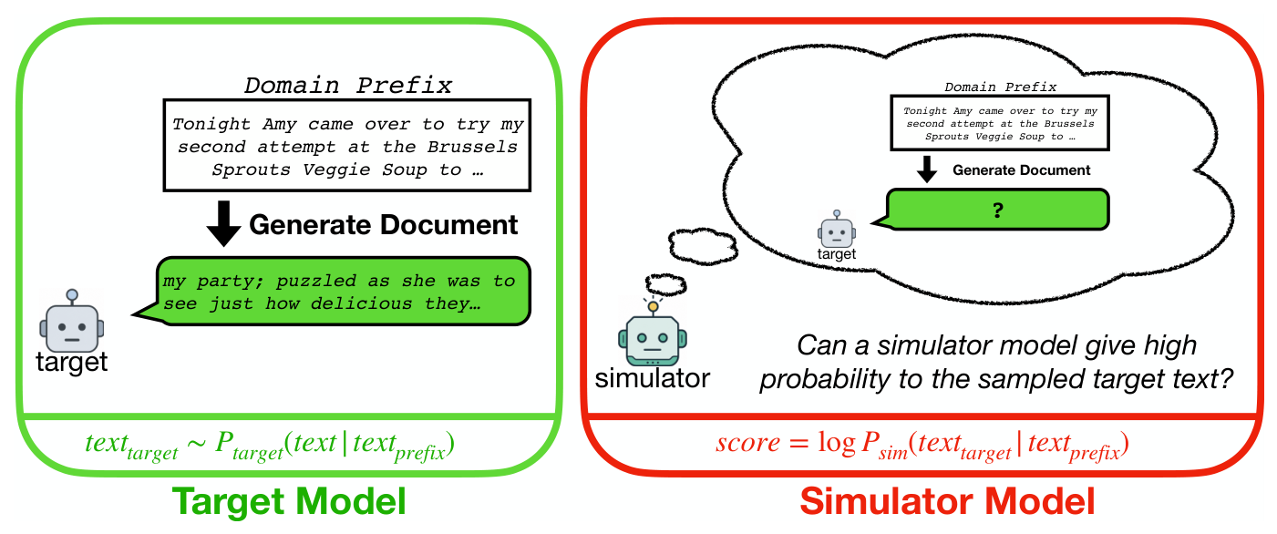
Figure 3.
The best scorers for each generator, plotted by the log size (in 100m parameters) of the scorer vs. generator model. The main results (left) cover generations using prefixes from the broad-domain Pile corpus. This largely supports scale affinity, with the best scorers almost always similar in size to the generator, rather than simply the largest model. Also included (right) are equivalent experiments on specific domains, showing scale affinity to varying degrees. Triangular and circular markers distinguish in-family and out-of-family scorers.
Figure 3.
The best scorers for each generator, plotted by the log size (in 100m parameters) of the scorer vs. generator model. The main results (left) cover generations using prefixes from the broad-domain Pile corpus. This largely supports scale affinity, with the best scorers almost always similar in size to the generator, rather than simply the largest model. Also included (right) are equivalent experiments on specific domains, showing scale affinity to varying degrees. Triangular and circular markers distinguish in-family and out-of-family scorers.
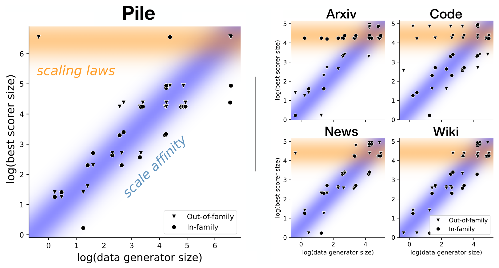

Table 1.
Examples of generated tokens (highlighted) for which a large model was significantly worse at predicting than a similarly-sized one. is the difference in loss between model m and the generator. In the first example, the model shows high agreement with the generator (small difference in loss), even though the given token indicates a mathematical mistake, which the model disagrees with (much higher loss).
Table 1.
Examples of generated tokens (highlighted) for which a large model was significantly worse at predicting than a similarly-sized one. is the difference in loss between model m and the generator. In the first example, the model shows high agreement with the generator (small difference in loss), even though the given token indicates a mathematical mistake, which the model disagrees with (much higher loss).
| text | ||
|---|---|---|
| the greatest common factor of 18 and 6024? 18 | 11.77 | 0.67 |
| When given an omnipotent voice, we can surely are not referring to | 21.73 | 10.84 |
| media often results in soft-faced transparency incott, Balanced | 14.04 | |
| Jim Palmer, the BBSE Cheese Foundation’s executive director, CBMPP00n | 8.34 | |
| details on this group when I have more the Mustang Retread Neos | 14.16 | 5.08 |
Disclaimer/Publisher’s Note: The statements, opinions and data contained in all publications are solely those of the individual author(s) and contributor(s) and not of MDPI and/or the editor(s). MDPI and/or the editor(s) disclaim responsibility for any injury to people or property resulting from any ideas, methods, instructions or products referred to in the content. |
© 2026 by the authors. Licensee MDPI, Basel, Switzerland. This article is an open access article distributed under the terms and conditions of the Creative Commons Attribution (CC BY) license (http://creativecommons.org/licenses/by/4.0/).
Copyright: This open access article is published under a Creative Commons CC BY 4.0 license, which permit the free download, distribution, and reuse, provided that the author and preprint are cited in any reuse.