
Submitted:
23 September 2026
Posted:
24 September 2026
You are already at the latest version
Abstract
Infrared focal-plane arrays are affected by pixel-to-pixel response variation, stripe artifacts, and random noise, which can impair image interpretation and target tracking in rapidly changing scenes. This study presents a symmetry-aware, scene-based non-uniformity correction method for real-time infrared image enhancement. The method forms a local reference with a cross-shaped four-neighborhood operator that weights the horizontal and vertical directions equally and is invariant to 90° rotations. This directional symmetry provides a balanced estimate of the local response, while per-pixel gain and offset coefficients are updated by gradient descent to reduce the difference between the corrected response and the local reference. The method was implemented on a 640 × 512 field-programmable gate array prototype. Hardware tests over 1000 frames yielded a processing latency below 1 ms per frame. On 12 datasets at a high noise level, the proposed method achieved a mean peak signal-to-noise ratio of 26.15 dB and a mean structural similarity index of 0.73, exceeding the strongest baseline by 0.78 dB and 0.05, respectively. Experiments on real non-uniform infrared sequences further showed effective suppression of stripe and random noise while preserving edges and background brightness. These results indicate that local directional symmetry is a useful design prior for efficient infrared non-uniformity correction and supports deployment on vehicle-, ship-, and airborne imaging platforms.
Keywords:
infrared imaging
; non-uniformity correction
; local spatial symmetry
; four-neighborhood filtering
; FPGA
; real-time image enhancement
1. Introduction
The detector and processing circuits of an infrared imaging system jointly determine the quality of the acquired images. In many practical scenes, the temperature difference between a target and its background is small, producing low contrast and a low signal-to-noise ratio. Pixel-to-pixel response variation in the focal-plane array can further introduce fixed-pattern noise and stripe artifacts. These degradations make subsequent feature extraction, recognition, and tracking more difficult; therefore, real-time correction methods must suppress non-uniformity without blurring weak edges or altering the background brightness.
Infrared image non-uniformity correction methods can be broadly divided into calibration-based, scene-based, and learning-based approaches. Calibration-based methods, such as two-point correction, require a reference radiation source and periodic interruption of normal operation [1]. Scene-based methods estimate correction parameters directly from the acquired sequence. Temporal high-pass filtering can reduce fixed-pattern noise [2], but low-frequency scene content may be misclassified as noise, causing ghosting. Bilateral filtering [3] and spatial low-pass/temporal high-pass filtering [4] alleviate this problem, while constant-statistics methods provide another important scene-based framework [5]. Learning-based methods have also been investigated, including shallow neural networks [6,7], bilateral-filter-assisted networks [8], residual architectures [9,10], and deep networks trained with simulated stripe noise [11]. Nevertheless, these approaches may still suffer from residual non-uniformity, over-smoothing, weak scene adaptability, or computational cost that limits hardware deployment.
The dominant source of fixed-pattern noise is the non-identical response of detector elements to the same incident radiance. A first-order model separates this variation into a multiplicative gain term and an additive offset term. Manufacturing tolerances, readout electronics, bias conditions, and temperature drift can change both terms, so a calibration obtained at one operating point may become inaccurate during long-term operation. The resulting artifacts often appear as stationary rows, columns, or pixel-wise patterns superimposed on a moving scene. Their spatial persistence makes them visually salient even when their amplitude is small, and their temporal evolution makes a single factory calibration insufficient for many vehicle-, ship-, and airborne applications.
Calibration-based non-uniformity correction remains attractive because two or more uniform radiance measurements provide a direct estimate of detector response. Its weakness is operational: a shutter or blackbody reference must occupy the optical path, and correction quality degrades as the detector drifts away from the calibration state. Scene-based methods instead exploit spatial or temporal redundancy in ordinary image sequences. Constant-statistics and temporal high-pass methods can operate continuously, but they face a fundamental separation problem because genuine low-frequency scene content and slowly varying detector bias occupy overlapping bands. If the update responds too quickly, scene structures leak into the coefficient maps and produce ghosting; if it responds too slowly, the method cannot follow detector drift.
Deep learning can learn more complex spatial priors than a hand-designed local filter, but network depth, memory traffic, quantization, and the availability of representative training pairs complicate embedded deployment. A model trained on one detector or noise distribution may also generalize poorly when the optics, ambient temperature, or readout chain changes. For the present application, the principal design objective is therefore not maximum capacity but a transparent update rule that can be evaluated per pixel, uses a small deterministic neighborhood, and maps efficiently to a streaming hardware pipeline. This objective favors a lightweight scene-based estimator whose operations and failure modes can be analyzed directly.
Real-time performance must be considered together with correction quality. A 640 × 512 frame contains 327,680 pixels, and every pixel must be acquired, corrected, enhanced, and transmitted within the frame period. Frame buffering and iterative optimization over an entire image would increase latency and external-memory traffic. In contrast, a local operator can be calculated as soon as the necessary neighboring samples are present in line buffers. A recursive gain/offset update can then reuse the coefficient state from the preceding frame. Such a design has constant work per pixel and is compatible with deep pipelining on a field-programmable gate array (FPGA).
Symmetry provides a useful way to describe balanced relationships in structured data. Prior studies have examined symmetry-related regularity in network topology through edge connectivity, ordered and Hamiltonian digraphs, orientations of complete bipartite graphs, and fault-tolerant embeddings [22,23,24,25], as well as in spatiotemporal graph-attention modeling [26]. For infrared correction, the relevant concept is local rather than global symmetry: the scene itself need not be mirror-symmetric, but the estimation operator should treat opposite horizontal and vertical neighbors consistently. A cross-shaped four-neighborhood has equal weights in the four cardinal directions and is unchanged by 90° rotation. In locally smooth regions, this directional balance provides a stable reference; detector-induced row or column deviations disrupt that balance and can therefore be reduced through iterative gain and offset correction.
The term symmetry is used in several different senses in imaging, and this distinction is important. Global bilateral symmetry describes similarity between large mirrored parts of an object; many natural infrared scenes do not satisfy that condition. The present method instead concerns operator symmetry. The four-neighborhood stencil assigns identical coefficients to the upper, lower, left, and right samples. Its response is unchanged when those samples are permuted by a quarter-turn rotation, and opposite directions contribute equally to the local estimate. This weak, local prior does not prescribe the shape of the target. It only prevents the correction rule itself from favoring one cardinal direction before image evidence is considered.
The central hypothesis is that an orientation-balanced reference provides a more neutral error signal than a one-sided or axis-specific estimate when fixed-pattern noise is superimposed on locally correlated scene content. The hypothesis is evaluated at the level of the complete correction system through full-reference PSNR and SSIM measurements, visual comparisons on real non-uniform sequences, and FPGA timing. The available experiments do not isolate every component of the stencil; accordingly, the symmetry interpretation is presented as a mechanistic explanation of the estimator rather than as proof that symmetry alone accounts for all performance gains.
Motivated by this observation, this paper combines scene-based non-uniformity correction with real-time infrared image enhancement. The main contributions are: (1) a symmetry-aware local reference based on an equally weighted four-neighborhood; (2) per-pixel gain and offset adaptation using gradient descent; (3) an FPGA implementation for 640 × 512 infrared video with sub-millisecond latency; and (4) quantitative and visual comparisons with guided filtering, median histogram equalization (MHE), bilateral-filter-based temporal high-pass filtering (BFTH), and fast non-local means (Fast-NLM).
2. Infrared Imaging System and Problem Definition
An infrared imaging device collects the thermal radiation emitted by all objects within a scene via an infrared optical system and projects it onto the focal plane of an infrared detector assembly. The main components of an infrared imaging device typically comprise an infrared optical lens, structural parts, an infrared detector assembly, and an imaging hardware system, as shown in Figure 1 below. In this paper, a non-uniformity correction algorithm is implemented based on a Field Programmable Gate Array (FPGA) prototype infrared photoelectric detection system, enabling rapid functional verification.
2.1. Structural Components
The structural components consist mainly of the system's main frame, lens structure, connectors, and other parts. These are used to assemble and integrate the infrared detector assembly, imaging hardware system, and optical system and to fix them in place with external systems.
Mechanical stability is relevant to correction because small changes in detector position, optical alignment, or thermal contact can alter the apparent spatial pattern. The structure must therefore maintain the registration between the detector array and the streamed coefficient maps. It must also conduct heat predictably and avoid obstructing the electrical interfaces used for detector timing and image output. These constraints do not change the mathematical update rule, but they determine whether a coefficient associated with coordinate (i, j) continues to represent the same physical detector element during operation.
2.2. Infrared Detector Assembly
The function of the infrared detector assembly is to receive thermal radiation energy information from the target scene that the infrared optical system converges and convert it into electrical signals of corresponding intensities. This assembly is the key core unit of the infrared imaging device, which outputs raw infrared images for subsequent processing by the imaging hardware system [12,13,14].
The array converts incident thermal radiation into electrical responses that are sampled by the readout circuit. Even under spatially uniform illumination, two pixels may produce different digital values. Moreover, the relative difference can vary with integration time and temperature. In the linear model adopted in this work, these deviations are represented by per-pixel gain and offset coefficients. Higher-order response nonlinearity is outside the model; consequently, the proposed correction is most appropriate over an operating range in which the detector response can be approximated locally by an affine relation.
2.3. Imaging Hardware System
The imaging hardware system is composed of multiple signal acquisition and conditioning circuits, image processing and control circuits, and peripheral power supplies. The system's primary functions include regulating the output timing of the infrared detector assembly, conditioning, and the collection of multiple analogue voltage outputs from the detector assembly. Additionally, it employs an image processing core processor to facilitate image processing and output, as well as to enable communication and signal exchange with external control units [15,16,17].
The image-processing core is positioned after signal acquisition and before the external image interfaces. This placement gives the correction stage access to the raw spatial arrangement of detector samples and allows the corrected stream to feed both digital and analogue output paths. The FPGA is particularly suitable for the design because neighborhood generation, arithmetic, coefficient memory, and interface control can operate concurrently. The four-neighborhood mean requires only adjacent rows and columns; therefore, it can be implemented with line buffers rather than repeated full-frame reads.
2.4. Problem Formulation and Design Requirements
Let Xₖ be the raw frame at time k and let Yₖ be the corrected frame. The task is to estimate a spatially varying gain map Gₖ and offset map Oₖ such that detector-dependent variation is suppressed while scene-dependent contrast and edges remain visible. No uniform reference source is available during normal operation. The estimate must therefore be driven by relationships within the observed sequence. Because the desired clean radiance is unknown for real scenes, the method uses a local spatial reference as a surrogate target and updates the coefficients gradually across frames.
Four engineering requirements follow from this formulation. First, the correction must be online: frame k should be processed using the current samples and state retained from earlier frames. Second, the per-pixel computation must be bounded and regular so that the architecture can sustain a streaming rate. Third, the update must be stable; scene motion or an isolated high-contrast edge should not cause a large instantaneous change in gain or offset. Fourth, the reference estimator should avoid built-in directional preference. The last requirement motivates the symmetric cross-shaped stencil used in Section 3.3.
Correction and enhancement are related but distinct operations. Non-uniformity correction estimates detector response differences, whereas enhancement remaps the corrected signal for display and interpretation. Applying enhancement before correction can magnify stripes and defective-pixel patterns. The system therefore performs non-uniformity correction first and passes the resulting stream to the enhancement and output stages. Quantitative evaluation focuses on the correction output because PSNR and SSIM require a clearly defined reference, while the displayed examples additionally reveal contrast and edge behavior after the complete processing chain.
3. Materials and Methods
3.1. Processing Pipeline and Design Objectives
The processing pipeline comprises scene-based non-uniformity correction followed by image enhancement and hardware output. The correction stage estimates a local reference, computes the difference between the corrected pixel and that reference, and iteratively updates the gain and offset coefficients. The enhancement stage then improves the visibility of the corrected signal while preserving the dynamic range required by the output interface. The complete pipeline is mapped to the FPGA so that acquisition, correction, enhancement, and transmission can operate continuously, as illustrated in Figure 2.
The pipeline can be understood as a feedback estimator embedded in a feed-forward video path. For each incoming pixel, the forward path produces a corrected response using the current gain and offset. In parallel, the feedback path constructs a local reference and calculates an error. The coefficient state is then updated for use in the next frame. This temporal separation is important: allowing the newly calculated coefficients to affect other pixels in the same frame would introduce scan-order dependence, whereas retaining a complete coefficient state for frame k gives every coordinate a consistent update rule.
The neighborhood stage requires the upper, lower, left, and right samples around the center. In a raster stream, samples from previous rows are available through line buffers, while the right neighbor introduces a short look-ahead or pipeline delay. Once the stencil is available, the division by four in the reference calculation can be realized as a binary shift in fixed-point hardware. Multiplication is required for the gain term and for the gain update; addition and subtraction implement the offset, error, and coefficient accumulation. These operations are local and expose pixel-level parallelism.
The design separates algorithm latency from system frame rate. Latency measures the time between the availability of a required input sample or frame and the corresponding corrected output; throughput measures how frequently outputs can be produced once the pipeline is filled. The reported sub-millisecond value characterizes the implemented processing delay over 1000 frames. Interface overhead, sensor integration time, and display transmission are platform-dependent and should not be conflated with the arithmetic latency of the correction core.
3.2. Scene-Based Non-Uniformity Correction
The scene-based method does not require a blackbody reference or prior temperature information and can therefore update the correction parameters during continuous video acquisition. Its feedback structure contains an input layer, a calibration layer, a local-reference layer, and an output layer, as shown in Figure 3.
The four functional layers operate as follows:
1) The input layer receives the raw infrared pixel and its four cardinal neighbors.
2) The calibration layer applies the current gain and offset coefficients to the raw response.
3) The local-reference layer calculates the equally weighted four-neighborhood mean and feeds the resulting error back to the calibration layer.
4) The output layer applies the updated coefficients to produce the corrected pixel value.
The non-uniform response of each pixel in the infrared focal-plane array is modeled by the following linear relation:
yk(i,j) = gk(i,j) ⋅ xk(i,j) + ok(i,j)
The affine model is intentionally simple. A multiplicative deviation changes response sensitivity and is represented by gₖ(i, j), while an additive deviation shifts the response independently of incident signal and is represented by oₖ(i, j). The coefficients in Equation (1) are correction coefficients rather than factory-measured detector parameters: they are updated so that yₖ(i, j) approaches the local reference. At initialization, a neutral state can be represented conceptually by unit gain and zero offset; subsequent frames refine that state as evidence accumulates.
In Equation (1), (i, j) denotes the pixel coordinates and k is the frame index. The variables gₖ(i, j) and oₖ(i, j) are the estimated gain and offset correction coefficients, respectively; xₖ(i, j) is the raw detector response; and yₖ(i, j) is the corrected response.
The local reference is obtained with the cross-shaped four-neighborhood operator:
The spatial stencil corresponding to Equation (2) is H = (1/4)[[0,1], [0,1], [0,1]], where the center coefficient is zero. Excluding the center prevents the same raw sample from appearing on both sides of the error calculation. The stencil estimates the local response from immediately adjacent pixels, which are likely to observe related radiance in smooth areas but carry independent detector-response deviations. A compact neighborhood also limits buffer size and avoids the large spatial support that can blur small targets.
In Equation (2), fₖ(i, j) is the local reference for pixel (i, j), computed from the raw responses of its upper, right, lower, and left neighbors. Equal weighting prevents either spatial axis from being favored.
The correction error is defined as the difference between the corrected response and the local reference:
ek(i,j) = yk(i,j) − fk(i,j)
The sign convention eₖ = yₖ − fₖ makes the update intuitive. If the corrected center response is larger than its neighborhood reference, eₖ is positive and the negative gradient reduces the relevant coefficient. If it is smaller, the sign reverses. Because both gain and offset are adapted, the model can respond differently to signal-dependent and signal-independent components of non-uniformity. Nevertheless, the two effects may be difficult to identify over a sequence with limited radiance variation; sufficient scene diversity remains beneficial for convergence.
In Equation (3), eₖ(i, j) is the correction error. The gain and offset coefficients are updated by gradient descent to minimize the squared error. The objective function is
Differentiating F with respect to gₖ(i, j) and oₖ(i, j) gives
Using the negative gradient direction, the coefficient increments are
The learning rate μ controls the trade-off between convergence speed and stability: a larger value accelerates adaptation but increases the risk of oscillation, whereas a smaller value improves stability but slows convergence.
The frame-to-frame updates of the gain and offset coefficients are therefore
The update is a stochastic-gradient step evaluated at each pixel and frame. Its computational appeal is that it does not require matrix inversion, batch optimization, or back-propagation through a deep network. The learning rate must be interpreted together with signal scaling. When xₖ is represented by a large integer range, the gain gradient contains the product xₖeₖ and can be much larger than the offset gradient. In fixed-point hardware, coefficient word length, scaling, saturation, and the selected μ therefore jointly determine numerical stability.
Scene motion has two competing roles. It changes the radiance incident on a detector element and thus provides the excitation needed to distinguish persistent detector bias from scene content. Excessively slow or absent motion, however, can make a true scene feature appear stationary and allow it to influence the coefficient state. Conversely, abrupt motion can create a large instantaneous error. The gradual recursive update reduces sensitivity to a single frame, but it does not eliminate this ambiguity. The qualitative tests with real sequences are consequently important complements to the synthetic full-reference measurements.
In Equation (7), μ is the adjustable learning rate. The updated coefficients are retained for the next frame, enabling continuous scene-based adaptation without interrupting image acquisition.
3.3. Symmetry Interpretation and Applicability
Define the four neighbor samples around a center as the ordered vector v = [xᵤ, xᵣ, x_d, x_l]ᵀ. A 90° rotation acts as a cyclic permutation P on v. The reference is f = (1/4)1ᵀv, where 1 is the all-ones vector. Since 1ᵀP = 1ᵀ, f(Pv) = f(v). Reflection across either image axis also only permutes the same four samples, so the reference is invariant to the dihedral transformations of the cross. This invariance is exact for the operator even when the four observed intensities are not equal.
The same property can be expressed through opposing pairs. Let h = (x_l + xᵣ)/2 and v̄ = (xᵤ + x_d)/2. Equation (2) is f = (h + v̄)/2: horizontal and vertical evidence has equal total influence. A purely horizontal estimator would respond differently after a quarter-turn, and a causal one-sided estimator could imprint raster orientation on the correction. Equal pair weighting does not guarantee that f is an unbiased estimate at an edge, but it removes an arbitrary directional preference from the estimator design.
The symmetry used here is a property of the estimator, not an assumption that the imaged scene is globally symmetric. Let R denote a 90° rotation about the center pixel. Because the four-neighborhood reference assigns a weight of 1/4 to each cardinal neighbor, applying R only permutes the four samples and leaves their mean unchanged. The operator is therefore rotationally symmetric over the cardinal directions and also balances the opposing horizontal and vertical pairs. This property reduces directional bias when estimating the local baseline and is particularly relevant to row- or column-structured fixed-pattern noise. At strong edges or fine asymmetric structures, however, a simple mean may mix samples from different regions. The gradual coefficient update limits abrupt changes, but an edge-aware or confidence-weighted symmetric operator is a worthwhile direction for future work.
3.4. Processing Procedure and Computational Characteristics
Algorithm 1 summarizes the frame-recursive procedure. The input consists of the raw frame Xₖ, the coefficient maps Gₖ and Oₖ retained from the previous state, and the learning rate μ. Neighborhood samples are generated in raster order. The local reference and corrected response are calculated independently for every valid coordinate, followed by the error and coefficient updates. The corrected response forms the output frame, while the updated maps become the state for frame k + 1.
| Algorithm 1. Symmetry-aware scene-based non-uniformity correction. | |
| Input | Raw frame Xₖ; coefficient maps Gₖ and Oₖ; learning rateμ |
| 1 | Generate the upper, right, lower, and left samples for pixel (i, j). |
| 2 | Compute the symmetric local reference fₖ(i, j) using Equation (2). |
| 3 | Compute the corrected response yₖ(i, j) using Equation (1). |
| 4 | Calculate eₖ(i, j) = yₖ(i, j) − fₖ(i, j). |
| 5 | Update gain gₖ₊₁(i, j) and offset oₖ₊₁(i, j) using Equation (7). |
| 6 | Write yₖ(i, j) to the corrected stream and retain the updated coefficients. |
| Output | Corrected frame Yₖ and coefficient state {Gₖ₊₁, Oₖ₊₁}. |
For an M × N frame, the algorithm performs a constant number of arithmetic operations at each coordinate and therefore has O(MN) time complexity. The coefficient state requires O(MN) storage for gain and offset maps. In a streaming realization, neighborhood formation requires O(N) line-buffer storage rather than an additional full image. This regular access pattern is more favorable for FPGA implementation than non-local search, multi-scale feature extraction, or iterative frame-level solvers.
The reference average uses four additions and a division by four, while the correction and update paths use multiplications and additions. These counts describe the arithmetic graph, not a fixed resource total: synthesis tools may share, pipeline, or map operations to dedicated DSP blocks depending on clock constraints and word length. Similarly, the sub-millisecond measurement establishes timing feasibility on the prototype but does not by itself report logic utilization or power. Those hardware quantities are addressed as reporting limitations in Section 5.5.
Border coordinates require a deterministic policy because not all four neighbors are available. Common implementations replicate the nearest valid sample, use only available neighbors with renormalized weights, or leave a one-pixel border unchanged. The archived manuscript did not retain which policy produced the reported tables; therefore, no unsupported choice is asserted here. For exact reproduction, the final code release or author-supplied implementation record should identify the border rule, coefficient initialization, fixed-point formats, saturation limits, and the numerical value of μ.
4. Experimental Setup and Results
4.1. Prototype and Evaluation Data
The method was implemented on a 640 × 512 FPGA prototype verification system, as shown in Figure 4. Timing was measured over 1000 test frames to evaluate the suitability of the design for continuous real-time processing.
The prototype contains the FPGA logic platform, an adapter board, a CPU interface board, and a detector/image-output board. The CPU interface supports program loading and debugging and exposes UART, I²C, and GPIO connections. The detector board supplies control and acquisition signals and routes Camera Link and PAL outputs. This modular arrangement permits the correction core to be exercised with the same interfaces used by the infrared imaging chain rather than only in an offline software simulation.
Quantitative experiments comprise 12 indexed datasets at the high noise level used in the original test campaign. Each dataset provides the corrected image and a corresponding reference required for PSNR and SSIM. Because the archived manuscript does not identify public dataset names, the sets are reported consistently as Sets 1–12. A separate collection of real infrared sequences containing genuine non-uniformity noise is used for visual evaluation, where a noise-free reference is unavailable. The distinction prevents full-reference scores from being implied for the practical sequences.
The proposed update is scene-based and does not require supervised parameter training. Accordingly, there is no learned train/test split analogous to a deep neural network. The sequence itself supplies the temporal observations used to adapt detector coefficients. For a fair comparison, all methods are evaluated on the same noisy inputs and references, and the metrics are calculated after mapping outputs to a common image range. Results are reported per dataset rather than only as a global average so that variability and unfavorable cases remain visible.
Hardware timing was evaluated over 1000 frames of size 640 × 512. The measured processing delay remained below 1 ms per frame. The experiment demonstrates repeatability of the latency observation over a sustained sequence; however, the available record does not provide FPGA clock frequency, synthesis constraints, resource utilization, external-memory bandwidth, or power. These omissions do not change the measured delay but limit cross-platform comparison and should be resolved in the reproducibility package accompanying submission.
4.2. Evaluation Protocol
4.2.1. Objective Metrics
Performance was assessed by visual inspection and by two full-reference objective metrics: peak signal-to-noise ratio (PSNR) and the structural similarity index (SSIM).
PSNR is defined as
In Equation (8), n is the image bit depth and MSE is the mean squared error, defined as
In Equation (9), X is the corrected infrared image, Y is the corresponding reference image without non-uniformity noise, and m and n are the image height and width, respectively. A higher PSNR indicates a smaller pixel-wise reconstruction error.
SSIM is defined as
SSIM(X,Y) = l(X,Y)∙c(X,Y)∙s(X,Y)
SSIM compares luminance, contrast, and structure; a value closer to 1 indicates greater structural similarity. The three components are
where μₓ and μᵧ are the mean intensities of X and Y, σₓ and σᵧ are their standard deviations, σₓᵧ is their covariance, and C₁, C₂, and C₃ are stabilizing constants that prevent division by zero.
4.2.2. Baseline Methods
PSNR and SSIM characterize complementary aspects of reconstruction. PSNR is determined by mean squared error and penalizes absolute pixel deviations; it is sensitive to intensity scaling and does not directly describe perceptual structure. SSIM compares local luminance, contrast, and covariance and is more responsive to edge and texture preservation. Reporting both metrics reduces the risk that a method appears favorable only because it optimizes one error notion. Visual evaluation remains necessary for artifacts such as background darkening, residual stripes, halos, and motion-related ghosting.
The proposed method was compared with four baselines: guided filtering, median histogram equalization (MHE), bilateral-filter-based temporal high-pass filtering (BFTH), and fast non-local means (Fast-NLM). Guided filtering and Fast-NLM are designed to suppress noise while retaining local structure; MHE improves contrast through histogram redistribution; and BFTH combines spatial edge preservation with temporal high-pass correction. The comparison therefore covers spatial filtering, histogram-based enhancement, temporal correction, and non-local denoising. Table 1 reports PSNR for 12 datasets at a high noise level.
4.3. Quantitative Comparison
The four baselines represent distinct assumptions. Guided filtering uses a local linear model to smooth noise while preserving edges indicated by a guidance image. MHE redistributes intensity statistics and can improve visibility without modeling temporal detector drift. BFTH uses bilateral filtering to protect spatial discontinuities while a temporal high-pass component estimates fixed-pattern behavior. Fast-NLM averages samples or patches with similar appearance and can preserve repeated texture, but its search and weighting are less regular than the proposed four-neighborhood computation. The proposed method differs by maintaining explicit gain and offset state for every detector coordinate.
The proposed method obtained the highest mean PSNR (26.15 dB). MHE ranked second at 25.37 dB, followed by Fast-NLM (24.63 dB), BFTH (23.41 dB), and guided filtering (22.54 dB). Thus, the proposed method improved the mean PSNR by 0.78 dB over the strongest baseline. It achieved the highest value on 10 of the 12 datasets; MHE was higher on datasets 4 and 5. These results indicate that the correction is effective and comparatively consistent across the tested data.
Across Sets 1–12, the proposed PSNR has a mean of 26.15 dB, a sample standard deviation of 1.30 dB, and a range from 24.04 to 28.41 dB. MHE has a slightly smaller standard deviation of 1.02 dB but a lower mean of 25.37 dB. Fast-NLM, BFTH, and guided filtering have larger dispersions of 1.99, 2.05, and 2.07 dB, respectively. The proposed method is therefore not the least variable method in an absolute sense, but it combines the highest mean with substantially less variation than three of the four baselines.
A dataset-level comparison gives a more nuanced result than the mean alone. The proposed method has the highest PSNR on 10 sets. MHE is higher on Set 4 by 0.95 dB and on Set 5 by 0.10 dB. In contrast, the proposed method exceeds the best competing score by 2.30 dB on Set 1, 1.41 dB on Set 7, and at least 0.45 dB on Sets 2, 3, 6, 9, and 10. The average margin against the strongest baseline selected separately for each set is 0.54 dB. Thus, the improvement is broad but not universal, and Sets 4 and 5 identify conditions that deserve targeted error analysis.
Relative to each fixed baseline across all 12 paired sets, the mean PSNR gains are 3.61 dB over guided filtering, 0.78 dB over MHE, 2.75 dB over BFTH, and 1.52 dB over Fast-NLM. Exploratory 95% paired t-intervals for these mean differences are [2.57, 4.65], [0.23, 1.33], [1.77, 3.72], and [0.66, 2.38] dB, respectively. These intervals summarize between-set variation; they should not be interpreted as population-level guarantees because the independence and sampling frame of the 12 sets are not fully documented.
To examine performance on practical data, the proposed method and the four baselines were also applied to infrared sequences containing real non-uniformity noise. Representative results are shown in Figure 5.
Figure 5a shows the input image with real non-uniformity noise. In Figure 5b, most non-uniformity is removed, but the background is noticeably darkened. Figure 5c–f avoid this global darkening. The enlarged regions show substantial residual non-uniformity in Figure 5c and blurred edges with loss of detail in Figure 5d. Figure 5e and Figure 5f provide better overall correction; compared with Figure 5e, Figure 5f retains sharper edges and stronger target-to-background contrast.
Table 2 reports SSIM for the same 12 high-noise datasets. The proposed method achieved the highest mean SSIM (0.73), followed by Fast-NLM (0.68), BFTH (0.65), guided filtering (0.64), and MHE (0.60). The gain of 0.05 over the strongest baseline is consistent with the visual observation that the proposed correction better preserves structural information.
The SSIM results are more uniform. The proposed method is strictly highest on 11 sets and tied with Fast-NLM at 0.70 on Set 4. Its values range from 0.65 to 0.79, with a mean of 0.733 and a standard deviation of 0.054. The paired mean improvement is 0.100 over guided filtering, 0.133 over MHE, 0.082 over BFTH, and 0.052 over Fast-NLM. The corresponding exploratory 95% paired t-intervals are [0.079, 0.121], [0.090, 0.177], [0.063, 0.101], and [0.029, 0.075]. Even the lower bound against the strongest SSIM baseline remains positive for these 12 sets.
PSNR and SSIM do not rank the baselines identically. MHE is the second-best method in mean PSNR but the weakest in mean SSIM, indicating that favorable pixel-wise error does not necessarily preserve local structure. Fast-NLM ranks second in SSIM and third in PSNR, which is consistent with its use of non-local similarity. The proposed method ranks first in both means. This joint behavior supports the claim that its correction reduces absolute error without sacrificing the structural relationships emphasized by SSIM.
4.4. Summary Statistics and Hardware Timing
At less than 1 ms, the processing delay occupies less than 6% of a 16.67 ms frame period at 60 frames/s and less than 3% of a 33.33 ms period at 30 frames/s. This comparison indicates substantial timing headroom for the correction stage. It does not imply that the complete camera produces 1000 frames/s, because detector integration, interface clocks, buffering, enhancement, and transmission impose additional limits. The appropriate conclusion is that the measured correction core is not the bottleneck at common video frame rates on the tested prototype.

Table 3.
Summary statistics over the 12 high-noise datasets.
| Method | PSNR (dB), mean ± SD | ΔPSNR (dB) | SSIM, mean ± SD | ΔSSIM |
|---|---|---|---|---|
| Proposed | 26.15 ± 1.30 | – | 0.733 ± 0.054 | – |
| Guided filter | 22.54 ± 2.07 | 3.61 | 0.633 ± 0.055 | 0.100 |
| MHE | 25.37 ± 1.02 | 0.78 | 0.599 ± 0.051 | 0.133 |
| BFTH | 23.41 ± 2.05 | 2.75 | 0.651 ± 0.056 | 0.082 |
| Fast-NLM | 24.63 ± 1.99 | 1.52 | 0.681 ± 0.050 | 0.052 |
The arithmetic regularity also benefits timing predictability. Unlike a data-dependent non-local search, the four-neighborhood path has the same local computation for every interior pixel. Once the pipeline is filled, coefficient updates can proceed in scan order with fixed scheduling. Deterministic scheduling is valuable in closed-loop imaging platforms, where worst-case latency and synchronization with detector timing can matter more than average software runtime.
Overall, the quantitative and visual results show that the proposed method suppresses non-uniformity without the pronounced background darkening, loss of detail, or edge blurring observed in several baselines. The average processing latency remained below 1 ms across 1000 test frames, supporting real-time FPGA deployment. Because the experiments cover 12 high-noise datasets and representative real sequences, broader validation across detector types, temperatures, and motion conditions remains necessary.
5. Discussion
5.1. Interpretation of the Correction Mechanism
The results can be interpreted through the interaction of three design choices: local spatial estimation, explicit detector-coordinate state, and slow temporal adaptation. The local mean supplies an immediate reference without a blackbody source. The gain and offset maps retain information tied to physical detector coordinates rather than only filtering the current frame. Temporal recursion prevents every local deviation from being accepted as a new calibration value. Together, these features address both spatially structured artifacts and drift across the sequence.
Directional symmetry contributes by making the reference independent of an arbitrary cardinal orientation. Row and column artifacts are common manifestations of readout-channel variation. A stencil that systematically favors a row or a causal scan direction can interact with those artifacts, whereas the cross operator assigns the same total weight to both axes. This does not remove all scene bias: at a horizontal edge, the vertical pair may straddle two regions, and at a vertical edge the horizontal pair may do so. The benefit is therefore best described as removal of estimator-induced orientation bias, not immunity to edge contamination.
The difference between PSNR and SSIM rankings illustrates this point. MHE attains competitive PSNR on several sets but has the lowest mean SSIM, suggesting that intensity redistribution can reduce numerical error while altering local structure. The proposed method's stronger SSIM indicates better preservation of relationships among neighboring pixels. Because the symmetry prior is defined on those relationships, SSIM is especially relevant; nevertheless, the evidence concerns the complete method, and a controlled stencil ablation is required to assign a separate effect size to symmetry.
5.2. Practical Significance
The method targets applications in which an infrared stream must remain available continuously. Eliminating periodic blackbody interruption is useful for tracking and situational-awareness systems because the scene is not temporarily obscured for recalibration. The sub-millisecond FPGA delay further supports insertion into an existing processing chain without consuming most of the frame budget. The local arithmetic graph is also amenable to fixed-point implementation and does not require an external accelerator or a stored training model.
Transparency is another practical advantage. Every output can be traced to the raw center pixel, four neighbors, stored coefficients, and learning rate. This facilitates hardware verification and safety review compared with a high-capacity learned model whose response may depend on many hidden activations. The same simplicity also constrains performance: a four-neighbor mean cannot represent complex textures, anisotropic edges, or non-linear detector response. The method should therefore be viewed as an efficient correction core rather than a universal restoration model.
5.3. Failure Cases and Robustness
Sets 4 and 5 are important because they prevent an overly broad claim. MHE exceeds the proposed PSNR by 0.95 and 0.10 dB on these sets, although the proposed SSIM is tied for best on Set 4 and clearly higher on Set 5. One plausible interpretation is that the intensity statistics of these sets favor histogram redistribution in mean squared error while the local structure remains better preserved by the proposed correction. Without the underlying scene labels and residual maps, this explanation remains a hypothesis. Future analysis should examine error images, edge-stratified scores, and scene motion for these two sets.
Static high-contrast edges are another potential failure mode. If a detector pixel repeatedly observes the same edge, the local reference may differ systematically from the center for scene-related reasons. Persistent error could then leak into the gain or offset estimate and create a faint ghost after motion. A smaller learning rate limits leakage but slows adaptation to genuine detector drift. Confidence gating based on temporal motion, gradient magnitude, or opposing-pair agreement could reduce updates at unreliable coordinates while preserving the symmetry of accepted neighborhoods.
5.4. Relationship to Broader Symmetry Research
The graph and network studies cited in [22,23,24,25,26] treat structural regularity in domains different from infrared imaging. Their relevance here is conceptual: symmetry constrains relationships under transformations and can reduce arbitrary degrees of freedom in a model. The present cross stencil is a small spatial graph centered on one detector element, with equal edge weights to four cardinal neighbors. Quarter-turn rotations and axis reflections act as node permutations that leave the aggregation unchanged. This graph interpretation makes the connection precise while avoiding the claim that results from network connectivity or financial forecasting directly validate infrared correction.
This perspective suggests extensions that remain faithful to the same principle. An eight-neighborhood operator could assign equal weights within symmetry orbits of the square grid; an edge-aware version could enforce equal treatment of opposing pairs while allowing data-dependent weights between axial and diagonal groups. A learned module could be constrained to be equivariant to rotations or reflections rather than relying on unconstrained convolution. These alternatives would increase modeling capacity, but their value should be established against the current four-neighbor baseline under identical hardware and data conditions.
5.5. Limitations and Reproducibility
Several limitations define the strength of the present conclusions. First, the 12 datasets are identified numerically but their source, scene categories, frame counts, bit depth, and high-noise generation parameters are not preserved in the manuscript. Second, baseline implementation sources and parameter values are unavailable. Third, the prototype result reports latency but not FPGA clock frequency, logic and memory utilization, DSP use, power, or maximum sustained input rate. Fourth, the real-sequence evaluation is visual and lacks a no-reference metric or expert rating protocol. These omissions should be addressed in the data and implementation package wherever records remain available.
The current comparison establishes performance of the complete proposed pipeline but does not include an ablation of neighborhood symmetry, separate gain-only and offset-only updates, or learning-rate sensitivity. Such experiments are particularly important for a symmetry-focused journal. A minimum ablation should compare the cross stencil with horizontal-only, vertical-only, one-sided causal, and eight-neighborhood references, report PSNR/SSIM and ghosting behavior, and measure any change in FPGA resources. Repeating measurements across detector temperatures and motion levels would further distinguish response drift from scene-induced error.
No claim is made that the method is optimal for every infrared detector or every scene. The evidence supports the narrower conclusion that, for the reported 12 high-noise sets and the tested real sequences, the complete symmetry-aware correction provides favorable reconstruction quality and can be implemented with sub-millisecond processing delay on the prototype. Public release of raw sequences, reference images, coefficient settings, and synthesis reports would allow independent verification and strengthen that conclusion.
6. Conclusions
This work presented a symmetry-aware, scene-based non-uniformity correction method for real-time infrared image enhancement. The method models each detector coordinate with adaptive gain and offset coefficients and constructs its reference from an equally weighted cross-shaped four-neighborhood. The reference is invariant to quarter-turn rotation and axis reflection because these transformations only permute neighbors with identical weights. Gradient-descent updates then reduce the difference between the corrected response and this local reference without requiring a blackbody interruption or supervised network training. The resulting computation is O(MN) for an M × N frame and has a regular streaming structure suitable for FPGA realization. On 12 high-noise datasets, the method achieved a mean PSNR of 26.15 ± 1.30 dB and a mean SSIM of 0.733 ± 0.054. It exceeded the strongest fixed baseline mean by 0.78 dB in PSNR and 0.052 in SSIM, produced the highest PSNR on 10 sets, and produced the highest SSIM on 11 sets with one tie. Real-sequence comparisons showed effective suppression of stripe and random noise while retaining sharper edges and background brightness. The 640 × 512 FPGA prototype maintained a processing delay below 1 ms over 1000 frames. These results demonstrate that local directional symmetry is a useful and hardware-efficient estimator constraint. Future work should add symmetry-specific ablations, edge-aware update confidence, complete cross-temperature validation, and public implementation records to establish generalization and reproducibility.
Funding
This research was funded by the National Science and Technology Major Project from Minister of Science and Technology, China, under Grant 2018AAA0103100.
Institutional Review Board Statement
Not applicable.
Informed Consent Statement
Not applicable.
Data Availability Statement
The data supporting the findings of this study are available from the corresponding author upon reasonable request, subject to institutional and project restrictions.
Conflicts of Interest
The authors declare no conflict of interest.
References
- Zhou, H.; Li, Q.; Liu, S.; et al. Nonuniformity and Its Correction Principle of Infrared Focal Plane Arrays. Laser Infrared 2003, 3, 46–48. [Google Scholar]
- Scribner, D.A.; Sarkady, K.A.; Kruer, M.R.; et al. Adaptive Nonuniformity Correction for IR Focal-Plane Arrays Using Neural Networks. Proceedings of SPIE, 1991; pp. 100–109. [Google Scholar] [CrossRef]
- Zuo, C.; Chen, Q.; Gu, G.; et al. New Temporal High-Pass Filter Nonuniformity Correction Based on Bilateral Filter. Opt. Rev. 2011, 18, 197–202. [Google Scholar] [CrossRef]
- Qian, W.; Chen, Q.; Gu, G. Space Low-Pass and Temporal High-Pass Nonuniformity Correction Algorithm. Opt. Rev. 2010, 17, 24–29. [Google Scholar] [CrossRef]
- Harris, J.G.; Chiang, Y.M. Nonuniformity Correction Using the Constant-Statistics Constraint: Analog and Digital Implementations. Proc. SPIE 1997, 3061, 895–905. [Google Scholar] [CrossRef]
- Kuang, X.; Sui, X.; Chen, Q.; et al. Single Infrared Image Stripe Noise Removal Using Deep Convolutional Networks. IEEE Photonics J. 2017, 9, 1–13. [Google Scholar] [CrossRef]
- Zhao, C.; Liu, Z. Improved Infrared Image Neural-Network Non-Uniformity Correction Algorithm. Infrared Laser Eng. 2013, 42, 1079–1083. [Google Scholar]
- Zhang, L.; Dong, F.; Fu, Y. Non-Uniformity Correction for Infrared Images Using Neural Networks. Infrared Technol. 2018, 40, 164–169. [Google Scholar]
- Mou, X.; Lu, J.; Zhou, X.; et al. Single-Frame Infrared Image Adaptive Correction Algorithm Based on a Residual Network. In Frontier Research and Innovation in Optoelectronics Technology and Industry; 2018; pp. 17–23. [Google Scholar] [CrossRef]
- Mou, X.; Lu, J.; Zhou, X. Adaptive Correction Algorithm of Infrared Images Based on an Encoding–Decoding Residual Network. Infrared Technol. 2020, 42, 833–839. [Google Scholar] [CrossRef]
- He, Z.; Cao, Y.; Dong, Y.; et al. Single-Image-Based Nonuniformity Correction of Uncooled Long-Wave Infrared Detectors: A Deep-Learning Approach. Appl. Opt. 2018, 57, D155–D164. [Google Scholar] [CrossRef] [PubMed]
- Lu, H.; Liu, Z.; Pan, X. An Adaptive Detail Equalization for Infrared Image Enhancement Based on Multi-Scale Convolution. IEEE Access 2020, 8, 156763–156773. [Google Scholar] [CrossRef]
- Xu, Y.; Liang, K.; Xiong, Y.; Wang, H. An Analytical Optimization Model for Infrared Image Enhancement via Local Context. Infrared Phys. Technol. 2017, 87, 143–152. [Google Scholar] [CrossRef]
- Xu, K.; et al. HFMNet: Hierarchical Feature Mining Network for Low-Light Image Enhancement. IEEE Trans. Instrum. Meas. 2022, 71, 1–14, Art. 5014014. [Google Scholar] [CrossRef]
- Li, S.; Jin, W.; Li, L.; Li, Y. An Improved Contrast Enhancement Algorithm for Infrared Images Based on Adaptive Double-Plateaus Histogram Equalization. Infrared Phys. Technol. 2018, 90, 164–174. [Google Scholar] [CrossRef]
- Wang, Y.; Cai, J.; Zhang, D.; Chen, X.; Wang, Y. Nonlinear Correction for Fringe Projection Profilometry with Shifted-Phase Histogram Equalization. IEEE Trans. Instrum. Meas. 2022, 71, 1–9, Art. 5005509. [Google Scholar] [CrossRef]
- Thomas, G.; Flores-Tapia, D.; Pistorius, S. Histogram Specification: A Fast and Flexible Method to Process Digital Images. IEEE Trans. Instrum. Meas. 2011, 60, 1565–1578. [Google Scholar] [CrossRef]
- Huang, S.-C.; Cheng, F.-C.; Chiu, Y.-S. Efficient Contrast Enhancement Using Adaptive Gamma Correction with Weighting Distribution. IEEE Trans. Image Process. 2013, 22, 1032–1041. [Google Scholar] [CrossRef] [PubMed]
- Zheng, Z.; Gao, J.; Mo, J.; Zhang, L.; Zhang, Q. A Fast Self-Correction Method for Nonlinear Sinusoidal Fringe Images in 3-D Measurement. IEEE Trans. Instrum. Meas. 2021, 70, 1–9, Art. 1006509. [Google Scholar] [CrossRef]
- Ibrahim, H.; Kong, N.S.P. Brightness Preserving Dynamic Histogram Equalization for Image Contrast Enhancement. IEEE Trans. Consum. Electron. 2007, 53, 1752–1758. [Google Scholar] [CrossRef]
- Fan, Z.; Bi, D.; Xiong, L.; Ma, S.; He, L.; Ding, W. Dim Infrared Image Enhancement Based on a Convolutional Neural Network. Neurocomputing 2018, 272, 396–404. [Google Scholar] [CrossRef]
- Wang, S.; Wang, M. The Edge Connectivity of Expanded k-Ary n-Cubes. Discret. Dyn. Nat. Soc. 2018, 2018, 7867342. [Google Scholar]
- Wang, M.J.S.; Yuan, J.; Lin, S.W.; et al. Ordered and Hamilton Digraphs. Chin. Q. J. Math. 2010, 25, 317–326. [Google Scholar] [CrossRef]
- Zhao, L.; Wang, M.; Zhang, X.; Lin, Y.; Wang, S. An Algorithm for the Orientation of Complete Bipartite Graphs. In Proceedings of the 2017 International Conference on Applied Mathematics, Modelling and Statistics Application (AMMSA 2017), 2017; pp. 361–364. [Google Scholar]
- Wang, S.; Wang, M.; Qi, Z.; Ren, Y. Embedding Paths into the 4-Ary n-Cube with Faulty Nodes. In Proceedings of the 2011 International Conference on Consumer Electronics, Communications and Networks (CECNet), 2011; pp. 4949–4951. [Google Scholar]
- Wei, Z.-L.; An, H.-Y.; Yao, Y.; Su, W.-C.; Li, G.; Saifullah; Sun, B.-F.; Wang, M.-J.-S. FSTGAT: Financial Spatio-Temporal Graph Attention Network for Non-Stationary Financial Systems and Its Application in Stock Price Prediction. Symmetry 2025, 17, 1344. [Google Scholar] [CrossRef]
Figure 1.
Block diagram of the infrared imaging hardware system.
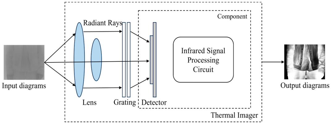
Figure 2.
Architecture of the non-uniformity correction and infrared image enhancement pipeline.
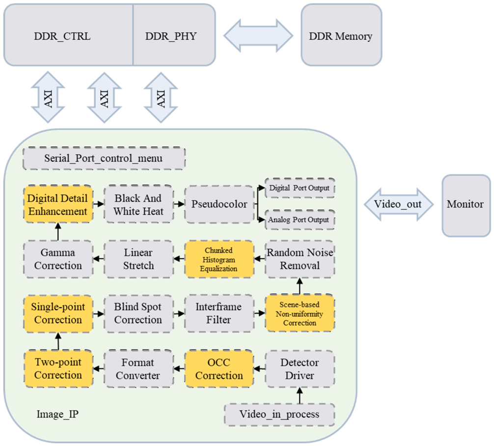
Figure 3.
Feedback structure of the scene-based correction method.
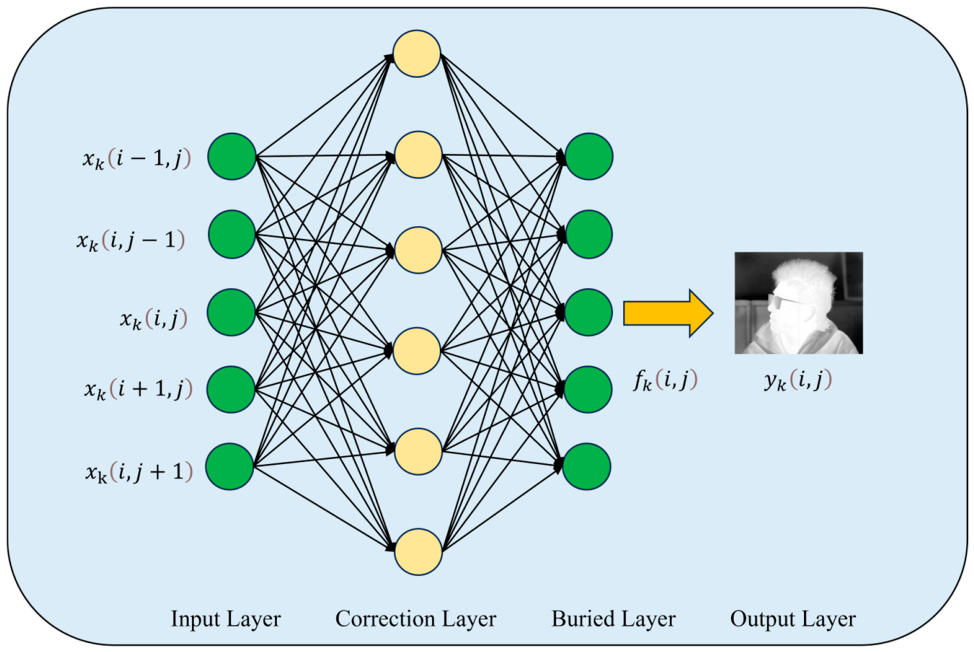
Figure 4.
FPGA prototype verification system: (a) S7-13P Prodigy Logic System (Single-VU13P); (b) P-PM-FMCHPC-V2.0 adapter board connected to the J1 and J2 ports; (c) CPU interface board for program loading, debugging, and peripheral outputs (UART, I²C, and GPIO); and (d) detector and image-output board for detector control, Camera Link output, and PAL output.
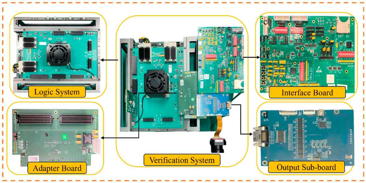
Figure 5.
Correction results produced by the compared methods.
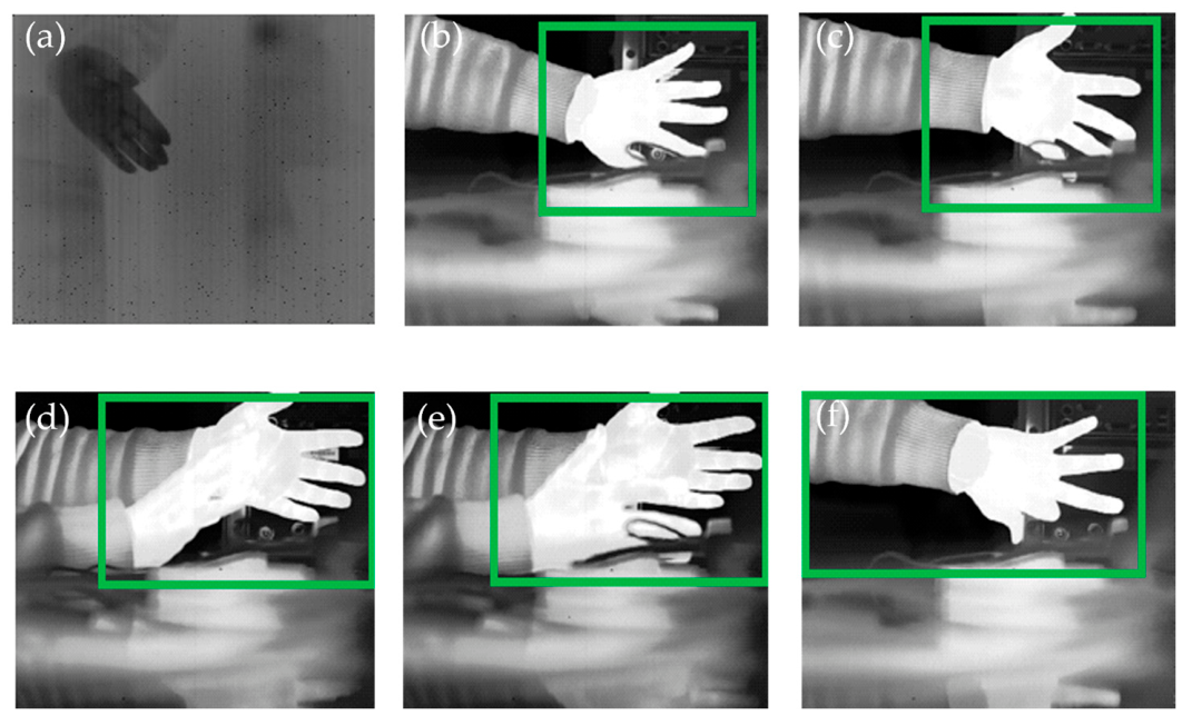
Table 1.
PSNR (dB) for 12 datasets in the random-noise reduction experiment at a high noise level.
| Set | Proposed | Guided filter | MHE | BFTH | Fast-NLM |
|---|---|---|---|---|---|
| 1 | 26.56 | 21.09 | 24.26 | 21.65 | 22.75 |
| 2 | 28.12 | 24.82 | 26.48 | 26.10 | 27.43 |
| 3 | 26.40 | 21.78 | 25.95 | 22.72 | 23.97 |
| 4 | 24.43 | 21.62 | 25.38 | 22.68 | 24.19 |
| 5 | 25.31 | 19.84 | 25.41 | 21.29 | 23.20 |
| 6 | 25.32 | 20.87 | 24.51 | 21.50 | 22.70 |
| 7 | 26.23 | 19.72 | 24.82 | 20.82 | 22.54 |
| 8 | 28.41 | 26.11 | 26.87 | 27.14 | 28.34 |
| 9 | 24.04 | 22.57 | 23.23 | 23.01 | 23.06 |
| 10 | 26.40 | 23.68 | 25.80 | 24.31 | 25.56 |
| 11 | 26.77 | 24.76 | 26.14 | 25.53 | 26.60 |
| 12 | 25.85 | 23.64 | 25.60 | 24.14 | 25.26 |
| Mean | 26.15 | 22.54 | 25.37 | 23.41 | 24.63 |
Table 2.
SSIM for 12 datasets in the random-noise reduction experiment at a high noise level.
| Set | Proposed | Guided filter | MHE | BFTH | Fast-NLM |
|---|---|---|---|---|---|
| 1 | 0.75 | 0.64 | 0.54 | 0.63 | 0.64 |
| 2 | 0.78 | 0.71 | 0.55 | 0.72 | 0.70 |
| 3 | 0.78 | 0.69 | 0.63 | 0.72 | 0.75 |
| 4 | 0.70 | 0.58 | 0.69 | 0.63 | 0.70 |
| 5 | 0.79 | 0.63 | 0.69 | 0.68 | 0.74 |
| 6 | 0.77 | 0.63 | 0.59 | 0.64 | 0.67 |
| 7 | 0.77 | 0.64 | 0.61 | 0.66 | 0.69 |
| 8 | 0.78 | 0.73 | 0.57 | 0.74 | 0.74 |
| 9 | 0.66 | 0.58 | 0.54 | 0.60 | 0.59 |
| 10 | 0.67 | 0.58 | 0.58 | 0.59 | 0.65 |
| 11 | 0.69 | 0.62 | 0.60 | 0.64 | 0.68 |
| 12 | 0.65 | 0.56 | 0.60 | 0.56 | 0.62 |
| Mean | 0.73 | 0.64 | 0.60 | 0.65 | 0.68 |
Disclaimer/Publisher’s Note: The statements, opinions and data contained in all publications are solely those of the individual author(s) and contributor(s) and not of MDPI and/or the editor(s). MDPI and/or the editor(s) disclaim responsibility for any injury to people or property resulting from any ideas, methods, instructions or products referred to in the content. |
© 2026 by the authors. Licensee MDPI, Basel, Switzerland. This article is an open access article distributed under the terms and conditions of the Creative Commons Attribution (CC BY) license (http://creativecommons.org/licenses/by/4.0/).
Copyright: This open access article is published under a Creative Commons CC BY 4.0 license, which permit the free download, distribution, and reuse, provided that the author and preprint are cited in any reuse.