

Submitted:
23 September 2026
Posted:
24 September 2026
You are already at the latest version
Preprints on COVID-19 and SARS-CoV-2
Abstract
This study presents a multi-instrument remote sensing approach to characterize the optical properties and vertical distribution of aerosols within the planetary boundary layer (PBL) over New York City during the COVID-19 pandemic and post-pandemic periods. The analysis focuses on changes in aerosol loading associated with variations in anthropogenic activity and examines the relationship between column-integrated aerosol optical properties, vertically resolved aerosol distributions, and near-surface fine particulate matter (PM2.5). Continuous ceilometer observations are used to characterize profiles of attenuated backscatter and to investigate aerosol vertical structure and variability within the PBL. These measurements are complemented by sun-photometer observations of column-integrated aerosol optical properties, radiosonde profiles of atmospheric thermodynamic structure, and ground-based PM2.5 measurements. The synergistic use of these datasets provides a more comprehensive characterization of aerosol optical and physical properties under varying meteorological and boundary-layer conditions than can be obtained from individual instruments alone. In addition, air-mass back trajectories calculated using the Hybrid Single-Particle Lagrangian Integrated Trajectory (HYSPLIT) model are employed to investigate the potential influence of local, regional, and long-range aerosol transport on observed aerosol variability over New York City. Comparisons between the pandemic and post-pandemic periods reveal substantial differences in aerosol loading and pollution levels, highlighting the combined influence of changes in anthropogenic emissions, PBL dynamics, meteorological conditions, and transported aerosol on the urban aerosol environment. The results demonstrate the value of integrating vertically resolved active remote sensing with columnar and surface observations and atmospheric transport modeling for assessing temporal changes in urban aerosol distributions and their controlling processes.
Keywords:
ceilometer
; extinction
; aerosol
; planetary boundary layer
; LIDAR
; environmental modeling
; aerosol optical depth
; aerosol transportation
1. Introduction
Since the Great London Fog, the influence of meteorological conditions, air quality, and pollutant emissions on public health has received sustained attention. Despite advances in air-quality management, rapid urbanization and industrialization continue to make urban air pollution a significant and persistent challenge (Wu et al., 2021; Via et al., 2021; Eleftheriadis et al., 2021; Mananga et al., 2023). Of particular concern is fine particulate matter with an aerodynamic diameter of ≤2.5 μm (PM2.5). These particles can penetrate deep into the respiratory system and enter the bloodstream, increasing the risk of respiratory and cardiovascular diseases, particularly among vulnerable populations (Mananga et al., 2023). In New York City, PM2.5 exposure from all sources is estimated to contribute annually to approximately 2,000 deaths and 5,150 emergency department visits and hospitalizations related to respiratory and cardiovascular disease (NYC Environmental & Health Data Portal, 2021). Similarly, a study in Rome reported that a 10 μg m−3 increase in PM2.5 concentration was associated with a 4% increase in the risk of nonaccidental mortality (Cesaroni et al., 2013).
This study evaluates aerosol and air-quality conditions over New York City during June–July 2020, representing the acute phase of the COVID-19 pandemic, and the corresponding period in 2023, representing post-pandemic conditions. The intervening years were excluded because partial pandemic restrictions remained in place. The effects of pandemic-related changes in anthropogenic activity on particulate pollution remain debated. Whereas Zangari et al. (2020) reported no significant changes in particulate pollution, Sarfraz et al. (2020) and Shehzad et al. (2021) identified substantial variations. These contrasting findings demonstrate the need for rigorous, localized analyses to quantify the influence of anthropogenic activity on urban air quality.
To characterize aerosol conditions and transport processes, this study employs a suite of complementary observations, including a Lufft CHM15k ceilometer. Lidar remote-sensing techniques provide high-resolution vertical information on aerosol distributions and transport pathways and are widely used for atmospheric particulate-matter monitoring (Vladutescu et al., 2012). Spaceborne lidar observations from CALIPSO, for example, have documented the horizontal and vertical evolution of pollution plumes over major urban areas, including Mexico City (Kar et al., 2015), while ground-based Doppler lidars have resolved fine-scale turbulence and pollutant dispersion in densely populated coastal environments (Arend et al., 2020). Multiwavelength elastic–Raman lidar techniques have further demonstrated the ability to retrieve aerosol and cloud properties simultaneously (Wu et al., 2011). Here, ceilometer-derived aerosol observations within the planetary boundary layer are used to assess the influence of human activity on air quality in New York City.
Lidar retrievals were performed using the Fernald algorithm, a widely applied inversion method for deriving aerosol extinction profiles from elastic-backscatter signals. The method solves the lidar equation by assuming a constant or parameterized lidar ratio and applying a boundary condition at a selected reference range, thereby estimating the vertical distribution of aerosols (Fernald et al., 1984). Building on the earlier work of Klett (1981), the Fernald approach provides a practical framework for aerosol retrieval under varying atmospheric conditions.
Interpretation of lidar-derived aerosol profiles requires consideration of planetary boundary layer (PBL) dynamics and chemistry. The planetary boundary layer height (PBLH) regulates the vertical distribution, mixing, and dispersion of air pollutants in urban environments. Relative to rural areas, urban PBL evolution is influenced by the urban heat-island effect, enhanced surface roughness, and anthropogenic heat emissions (Kim et al., 2021). These factors can promote a deeper and more turbulent daytime boundary layer, enhancing vertical mixing and temporarily diluting near-surface pollutant concentrations. In contrast, nighttime stabilization often produces a shallow PBL that confines pollutants near the surface and increases exposure risk (Jacobson, 2002). The PBLH exhibits pronounced diurnal variability and responds to wind speed, solar radiation, and cloud cover. Consequently, characterization of PBL dynamics is essential for interpreting aerosol lidar profiles and assessing urban air quality. Recent work has further demonstrated that the vertical distribution of wildfire smoke is strongly coupled to PBL behavior, including nocturnal boundary-layer collapse and daytime convective mixing (Huang et al., 2024).
Local emissions from road traffic, shipping, and aviation, as well as aerosols transported over long distances, can influence urban aerosol loading. Under stagnant conditions, locally emitted pollutants may dominate near-surface concentrations, whereas regional transport can introduce dust, wildfire smoke, and other aerosol types from distant source regions (Vladutescu et al., 2013). Atmospheric stratification can maintain elevated aerosol layers above the PBL; subsequent boundary-layer growth and entrainment may affect surface-level pollutant concentrations. Fine particles, including PM2.5 and black carbon, may therefore contribute to air-quality degradation through both local emissions and long-range transport processes (Hastie et al., 1993; Schumann, 1996).
The COVID-19 pandemic created an unprecedented opportunity to examine aerosol optical properties and atmospheric pollution under substantially reduced anthropogenic activity. Previous studies have reported that quarantine measures reduced emissions and improved urban air quality (Eleftheriadis et al., 2021). Consistent with these observations, the present study identifies aerosol-related differences of approximately a factor of two to three between the pandemic and post-pandemic periods. Although New York City’s initial stay-at-home order began on 20 March 2020, sparse data availability during March–May motivated the selection of June–July 2020 for the pandemic analysis and the corresponding months of 2023 for the post-pandemic comparison. New York City entered the first phase of reopening on 8 June 2020, following fulfillment of the State’s reopening criteria; occupancy restrictions and other safety protocols remained in effect during the study period.
The remainder of this paper is organized as follows. Section 2 describes the instrumentation and data sets. Section 3 presents the methodology and theoretical background. Section 4 provides the results and discussion, and Section 5 summarizes the main conclusions. The data used in this study are available from the City College of New York Data Server, NASA AERONET, the New York State Department of Environmental Conservation air-monitoring network, and the University of Wyoming atmospheric-sounding archive.
2. Instruments
The analysis integrates observations from a Lufft CHM15k ceilometer lidar, a CIMEL sun photometer, radiosondes, a 1405-DF TEOM ambient PM2.5 monitoring system, and HYSPLIT backward-trajectory simulations. These complementary data sets were used to characterize aerosol optical properties, vertical aerosol structure, local particulate-matter concentrations, and potential aerosol transport pathways.
2.1. Lufft CHM15k Ceilometer
The Lufft CHM15k is an autonomous, single-wavelength elastic-backscatter ceilometer lidar operating at 1064 nm (Wiegner et al., 2012, 2019). It measures range-resolved atmospheric backscatter signals to heights of up to 15 km, with a vertical resolution of 5–15 m, depending on the selected measurement range. The temporal resolution is configurable from 15 to 60 s. In addition to raw backscatter profiles, the instrument provides cloud-base height for up to nine cloud layers, penetration depth, maximum detection range, vertical visibility, sky-condition classification, and cloud amount.
The ceilometer comprises a laser transmitter, receiver, optical system, environmental sensors, and data-acquisition unit. The transmitter emits laser pulses with durations of 1–5 ns at a pulse repetition rate of 5–7 Hz and pulse energies of 7–9 μJ. The emitted beam is directed into the atmosphere through the optical system, and the receiver records the intensity of the radiation backscattered by atmospheric constituents as a function of time, from which altitude-resolved backscatter profiles are derived. Internal and external temperature sensors monitor instrument operating conditions. In this study, CHM15k backscatter observations were used to investigate cloud and aerosol vertical distributions, identify elevated plumes, and estimate the evolution of the planetary boundary layer.
2.2. CIMEL CE318-T Sun Photometer
The CIMEL CE318-T sun photometer measures direct solar irradiance at multiple wavelengths using spectral filters and silicon and InGaAs detectors. These measurements are used to derive aerosol optical depth (AOD), the Ångström exponent, and precipitable water vapor (PWV). The instrument deployed at the City College of New York (CCNY) campus is part of the NASA Aerosol Robotic Network (AERONET) (Holben et al., 1998) and is shown in Figure 1b.
The CE318-T consists of a control unit, optical sensors, a collimator, a robotic sun-tracking system, and a tripod. The collimator and robotic tracker maintain accurate alignment with the Sun to enable direct-sun irradiance measurements. The tracker operates over azimuth and zenith ranges of 0–360° and 0–180°, respectively, with an angular resolution of 0.003°. The instrument is equipped with nine spectral channels centered at 340, 380, 440, 500, 675, 870, 937, 1020, and 1640 nm, spanning the ultraviolet, visible, and near-infrared spectral regions. Solar irradiance measured sequentially through these filters is transmitted to the data-acquisition and processing unit, from which column-integrated aerosol and water-vapor properties are retrieved.
2.3. Radiosondes
Radiosonde observations were used to characterize the vertical profiles of atmospheric temperature, relative humidity, pressure, wind speed, and wind direction. Radiosondes are carried aloft by weather balloons, also known as sounding balloons, from the surface to the upper atmosphere. A typical radiosonde includes temperature, humidity, and pressure sensors, a Global Positioning System (GPS) receiver, and a transmitter. Operational upper-air soundings are commonly launched twice daily, at 00:00 and 12:00 UTC, providing globally consistent measurements of atmospheric structure. In this study, radiosonde data were obtained from the University of Wyoming Upper Air Soundings archive. The platform provides historical and near-real-time sounding data for stations worldwide and enables the selection of data by geographic region, station, date, and launch time. A representative radiosonde system is shown in Figure 1d.
2.4. TEOM 1405-DF Ambient Particulate-Matter Monitor
Ambient particulate-matter concentrations were measured using a Thermo Scientific Tapered Element Oscillating Microbalance (TEOM) 1405-DF system (Figure 1c). The TEOM 1405-DF provides continuous, near-real-time measurements of particulate-matter mass concentration. Depending on the sampling configuration, its dual-filter design can measure PM2.5 and either coarse particulate matter (PM10–2.5) or other particle-size fractions.
The instrument draws ambient air through a filter mounted on a tapered oscillating element. Particle accumulation on the filter increases the element mass and produces a measurable decrease in oscillation frequency. The measured frequency shift is converted to particulate-matter mass concentration, enabling high-temporal-resolution monitoring. Temperature and humidity control systems reduce measurement artifacts associated with water vapor and volatile particulate components. The TEOM 1405-DF is widely used for regulatory air-quality monitoring, long-term pollution-trend assessment, and exposure-related studies.
3. Methodology
The ceilometer measures the backscatter intensity of light in the time domain to determine cloud base height and aerosol backscatter profile. In this retrieval, we assumed a suitable LIDAR ratio and used the radiosonde data. Based on these, we find the extinction and backscatter coefficient by using Fernald’s method summarized below (Fernald, F. G., 1984). Further, we use the extinction coefficient to calculate the aerosol optical depth. Finally, we compare the difference in AOD between our results and the AERONET data. Hence, we apply the above procedures for two summer months to compare the differences between 2020 and 2023. Furthermore, we use the HYSPLIT MODEL for trajectory analysis, and CIMEL sunphotometer derived AOD to cross-validate and better understand the ceilometer’s measurements. This multi-instrument approach helps us verify and improve our understanding of atmospheric composition.
3.1. LIDAR Ratio, Backscatter, and Extinction
The LIDAR ratio is a crucial parameter in remote sensing and atmosphere studies. The LIDAR ratio is defined as the ratio of the particle extinction coefficient (α) and the particle backscattering coefficient (β) (Weitkamp, 2005). In our research, we assumed a LIDAR ratio of 40 sr at 1064-nm , a commonly used value for anthropogenic aerosols (Li, D. 2022; Omar et al., 2009).
The extinction coefficient is the sum of loss from absorption and light scattering. It refers to the reduction of the intensity of light as it propagates through the atmosphere due to scattering and absorption by particulates and gases. It quantifies how aerosols and gases affect the transmission of light, leading to phenomena such as haziness, reduced visibility, and color changes in the sky. High extinction values can indicate the presence of dense aerosols, clouds or pollutants. This presence effectively attenuates the LIDAR signal by absorption or scattering. In Eq. (1), the extinction coefficient is the sum of the scattering by molecules, scattering by particles, absorption by molecules, and absorption by particles.
Backscatter refers to the light that is reflected directly back to the LIDAR sensor after it interacts with atmospheric particles or molecules. It provides information about the properties and concentrations of aerosols and clouds. The strength and characteristics of the backscattered light help in determining particulate distribution and concentration, as well as in evaluating atmospheric conditions such as visibility and pollution levels. High backscatter values suggest the presence of larger or denser concentrations of particles, whereas lower backscatter values may indicate cleaner air or the presence of smaller particles. In Eq. (2), the backscatter coefficient is the sum of the backscatter by molecules and particles.
The Fernald method is a commonly used technique in LIDAR remote sensing to derive profiles of atmospheric backscatter and extinction coefficients from measured LIDAR signals. It assumes a known relationship between the backscatter and extinction (usually the LIDAR ratio) and requires a reference point in the atmosphere where the backscatter coefficient is known. Fernald explained the LIDAR equation, P(Z) is the return signal that is proportional to the received power from a scattering volume at a slant range Z as shown in Eq. (3)
Where E is the output energy pulse that is proportional to the transmitted energy; C is the calibration constant of the instrument, which includes losses in the transmitting and receiving optics and the effective receiver aperture; βpar(Z) and βmol(Z) are the backscattering cross sections of the aerosols and molecules at slant range Z, respectively. In this equation, , is the aerosol transmittance, and , is the molecular atmosphere transmittance. Additionally, (Z) and (Z) are the extinction coefficients of the aerosols and molecules at range Z, respectively. (Fernald et al. 1984)
According to the Fernald inversion method (Fernald, 1984), the aerosol backscatter coefficient is retrieved recursively from a selected reference altitude by solving the lidar equation in discrete form. Let denote the range-corrected signal and △Z the range resolution. A reference altitude Z(I) is selected in a relatively clean atmospheric region, where the aerosol backscatter coefficient is specified using an assumed scattering ratio as the boundary condition (here I represents the current iteration layer). Eq. (4) incorporates the effects of aerosol extinction between adjacent data points, range ΔZ apart. In this case is shown for the upper range, with the lower range being calculated similarly to determine ). Starting from the reference point , the total backscatter coefficient at the adjacent lower range gate is calculated using Eq. (5), while the value at the adjacent upper range gate is calculated using Eq. (6). In these equations, and represent the aerosol and molecular backscatter coefficients, respectively, and the exponential terms account for the molecular transmission correction between adjacent range gates.
After the aerosol backscatter coefficient is obtained, the corresponding aerosol extinction coefficient is derived using the assumed aerosol lidar ratio. The extinction-form recursive equations are given in Eq. (7) and (8), where and are the aerosol and molecular lidar ratios, taken as 40 sr and 8*3.14/3 sr, respectively. Eq. (7) gives the extinction-related solution for the lower range gate , while Eq. (8) gives the corresponding solution for the upper range gate . This backward and forward recursive procedure is applied to each individual time profile to retrieve the time-height distribution of aerosol backscatter and extinction coefficients.
To satisfy the inputs of Fernald method, the molecular backscatter is necessary (Geisinger et al. 2016). The backscatter coefficient by molecules is equal to the molecule number density (Eq. (9)) multiplied by the differential backscatter cross-section as in Eq. (10).
The molecule number density is equal to the pressure in Pascal divided by the product of Boltzmann constant k (k = 1.380649 × 10⁻²³ m2 kg s−2 K−1) and temperature in Kelvin (see Eq. (9)). The pressure and the temperature were retrieved from the BNL (90 km east of New York City) radiosonde readings available on the Atmospheric Soundings website at weather.uwyo.edu (University of Wyoming Atmospheric Soundings website).
This molecular number density was used in Eq. (10) to solve for the molecular backscatter coefficient . Because only two radiosondes measurements per day were available (00 and 12 UTC), the atmospheric profiles were interpolated to provide continuous input for the retrieval calculations.
Where is the scattering cross section of molecules at the given wavelength which according to Bucholtz’ look-up table (Bucholtz et al., 1995) is 2.734* 10−28 cm2 at wavelength 1100 nm (closest to the ceilometer wavelength of 1064 nm).
The Ceilometer calibration constant was implemented following the method proposed by O’Connor et al. (2004). In this procedure, an optically thick liquid cloud was selected as the calibration target. The liquid cloud lidar ratio (extinction/backscatter), , and the multiple-scattering correction factor, with values between 0.5 (thick optical clouds) and 1, in our case this factor is . Under the optically thick cloud assumption, the theoretical integrated attenuated backscatter,, can be expressed as Eq. (11) and represents the expected integrated backscatter for an opaque liquid cloud.
The measured integrated backscatter, β, was obtained by vertically integrating the measured range-corrected backscatter signal between the detected cloud base and cloud top and is given in Eq. (12). The calibration coefficient was then calculated as the ratio between the measured integrated backscatter and the theoretical integrated backscatter, as indicated in Eq. (13).
3.2. Aerosol Optical Depth
Aerosol optical depth is a measure of the extinction of solar radiation by aerosol particles in the atmosphere. It is defined as the vertical integration of the extinction coefficient.
An integrated AOD over CCNY is available through the NASA AERONET website for the CIMEL (Vladutescu et al. 2013), and retrieved from extinction profiles measured by the LIDAR.
3.3. NOAA HYSPLIT Trajectory Model
The Hybrid Single-Particle LaGrangeian Integrated (Trajectory HYSPLIT) model tracks movement of air masses either forward or backward. We used longitude and latitude for our location, 40.82131° N and 73.94904° W. Then, we used HYSPLIT to track the aerosol origins. Some important factors are altitude, rainfall, mixing layer height, etc. Therefore, with the help of this model we can track the aerosol movement into and out of the zone of interest.
The results and analysis of the measurements with the above instruments are given in the section 4, below.
4. Results and Analysis
In this section, we present some of the LIDAR vertical profile used in the analysis of the summer months of June and July of 2020 and 2023. We also validated the AOD retrievals using the CIMEL sunphotometer, and compared the backscatter signal to the PM2.5 measurements, and looked into the possible sources.
4. a. LIDAR Retrievals
The vertical profiles of calibrated range-corrected return signals for the months of June-July 2020 are illustrated in Figure 2. These profiles indicate that the signal between 15–24 UTC hours are strongly contaminated by solar background above the PBL in clear-air regions, requiring careful daily analysis and selection of a reference level with low to no aerosol load for accurate retrievals. The colorbar values indicate the attenuated backscatter coefficient (/km/sr) or calibrated range-corrected return signals.
The recorded lidar signals were further processed to retrieve vertical profiles of attenuated backscatter and derived aerosol extinction coefficients, as shown in Figure 3 and Figure 4. These figures illustrate aerosol-loading conditions observed during the 2020 and 2023 measurement periods. For each year, representative cases spanning relatively high aerosol loading to comparatively clean atmospheric conditions were selected: 10 June, 22 June, and 27 July 2020, and 1 June, 6 July, and 22 July 2023. Instrument power calibrations were corrected for the respective measurement periods. These cases demonstrate typical temporal variations in aerosol and cloud conditions.
As described in Section 3, the retrieval is based on the Fernald iterative inversion method, which requires selection of an appropriate molecular reference altitude. An unsuitable reference altitude can introduce artifacts and noise into the retrieved extinction and backscatter profiles. Therefore, reference regions were selected daily under relatively stable atmospheric conditions. Cloud-contaminated profiles were excluded before the extinction retrieval because clouds strongly attenuate and scatter the lidar signal, rendering aerosol retrievals within and below cloud layers unreliable. Cloud detections are identified by purple markers in the backscatter-profile figures. Figure 3 presents cases of enhanced aerosol backscatter (Figure 3a), moderate aerosol loading (Figure 3b), and relatively low aerosol loading (Figure 3c). A common color scale is used in all panels to enable direct comparison.
Sample selected days after the pandemic are illustrated in Figure 4 for June 1st, 2023 (Thursday), July 6th, 2023 (Thursday), and July 22nd, 2023 (Saturday).
The comparison of LIDAR retrieved AOD for 2023, indicates increased particulate pollution. We extended the comparison to cover two months (June and July). The LIDAR based aerosol optical depth was calculated for the entire duration of June and July of the two years and plotted for comparison in Figure 5. The retrieval approach is based on the methodology detailed in section three of the paper.
In this analysis, we applied a running average filter to remove noise, smoothen the strong transition between day and night, and to make it easier to observe trends in the data. The AOD relative difference was calculated based on the following formula:
Aerosol optical depth (AOD) values during summer 2023 were observed to be significantly higher than those observed during the corresponding period in 2020. Several elevated AOD episodes in June and July 2023 were associated with enhanced aerosol loading, including smoke transported from Canadian wildfire events. Some days identified as statistical outliers (see Section V) were also affected by intense precipitation, including 22 June 2023. Backscatter profiles for representative cases are presented in Figure 6. The profile for 7 June 2023 (Figure 6a) shows enhanced aerosol backscatter throughout much of the planetary boundary layer (PBL), consistent with the presence of transported wildfire smoke. In contrast, on 22 June, the ceilometer detected extensive cloud cover and rainfall; magenta markers indicate cloud-base altitude as determined by the proprietary Lufft software. The corresponding AOD time series shows elevated values before the precipitation event and missing retrievals during rainfall. This behavior is expected because precipitation and cloud cover strongly attenuate lidar signals and prevent reliable direct-sun AOD retrievals by the sun photometer used for cross-validation.
4. b. CIMEL Sunphotometer
Aerosol optical depth (AOD) measured by the CIMEL sun photometer at 1020 nm, the spectral channel closest to the 1064 nm operating wavelength of the ceilometer, is presented in Figure 7 for the two study periods. As noted previously, the CIMEL sun photometer and ceilometer are collocated on the roof of the Grove School of Engineering at The City College of New York (CCNY). The ceilometer-derived and CIMEL-derived AOD values exhibit similar temporal variability; however, the ceilometer-derived AOD is generally lower. This difference is expected because the ceilometer AOD is obtained by integrating aerosol extinction within the planetary boundary layer (PBL), whereas the sun photometer provides a column-integrated AOD measurement from the instrument location to the top of the atmosphere.
Differences between the two retrievals may also arise from their distinct measurement geometries. The sun photometer measures direct solar irradiance along a slant path toward the Sun, while the ceilometer samples the atmosphere along a near-vertical path. Consequently, the instruments may observe different, although spatially proximate, air masses, particularly at greater distances from the measurement site. Nevertheless, their overall temporal patterns are consistent. The lines connecting data points in Figure 7 are included solely as visual guides and do not represent continuous observations. Both instruments indicate higher AOD during June–July 2023 than during June–July 2020. In 2023, AOD frequently exceeded 1.0, whereas values in 2020 only rarely exceeded 0.4. Additional comparisons are provided in the Discussion section.
To investigate the origin and sources of the dense aerosols (such as June 7th and others), we performed backward trajectory analysis using the HYSPLIT model. The resulting trajectories are shown below. The backward trajectories corresponding to the two spikes observed in the LIDAR-retrieved AOD on June 7 and June 22 (Figure 6) are plotted in Figure 8a and Figure 8b, respectively. From Figure 8a, it is evident that the aerosols within the PBL predominantly originated from Canada, coinciding with particularly severe wildfire conditions during this period (Natural Resources Canada). Figure 8b illustrates clouds formed from aerosol plumes entering the PBL above New York City, within the altitude range of 0.5 km to 1.5 km, originating from outside the local PBL, specifically from northeastern regions of Canada. These aerosols in combination with the marine aerosols present at approximately 1.5 km altitude above the ocean, formed clouds which were transported over the city and precipitated towards the end of the day.
The trajectories clearly indicate that air parcels transported from Canadian regions underwent hygroscopic interactions and heterogeneous mixing with marine aerosols, resulting in cloud formation before being transported back inland as confirmed by the LIDAR vertical profiles illustrated in Figure 8b.
4. c. PM2.5 Measured by TEOM
As mentioned in section 2 of this paper, the PM2.5 data is available in near real-time on the Air Monitoring Website of the New York State Department of Environmental Conservation (NYSDEC). The averaged hour concentrations for the months of June and July of 2020 and 2023 are illustrated in Figure 9. The PM2.5 concentration units are in µg/m3 LC (Local Conditions depending on actual temperature and pressure at the sampling time). Note that the TEOM is located on top of the CCNY Administration building at an altitude of 10 m AGL.
It is already evident in the above figures that the anthropogenic aerosols concentrations are consistently higher in 2023 as compared to 2020. However, more analysis are conducted in the Discussion section.
5. Discussions
Figure 10 compares near-surface PM2.5 mass concentrations with aerosol backscatter measured by the ceilometer at 300 m above ground level (AGL) at CCNY. PM2.5 was measured at approximately 10 m AGL. Yellow-shaded intervals denote weekends, which generally exhibited lower aerosol loading, likely reflecting reduced anthropogenic activity. The two time series show similar temporal patterns, although several enhanced backscatter events were associated with Canadian wildfire smoke. These elevated aerosol layers were detected aloft before their influence was observed in near-surface PM2.5 concentrations. A dual-y-axis format was used to facilitate visual comparison of the two variables. Periods affected by clouds, precipitation, or transported wildfire smoke were excluded from the comparison. The remaining observations indicate a close correspondence between surface PM2.5 and lower-tropospheric aerosol backscatter, supporting the ceilometer retrievals and indicating higher aerosol loading during 2023.
The correlation between PM2.5 data and the Ceilometer backscatter data at 300 m AGL is illustrated in Figure 11. Data corresponding to special events, including transported wildfire smoke, cloud contamination, and rainfall episodes, were removed from the analysis.
The spread of PM2.5 concentration versus backscatter is broader at lower concentration levels and therefore the correlation of the 2020 parameters is much weaker compared to 2023. As the concentration increases, we can observe a stronger correlation between the two. As per Vladutescu et al. (2012), the mass density of anthropogenic aerosols is lower than that of natural aerosols. As per Table I of the mentioned paper, the aerosols produced through traffic and industrial activities, such as sulfate, ammonia, and nitrate have mass densities of 1.8 gm/cm3 being easily lofted to higher altitudes via convection processes and easily detectable at higher altitudes. On the other hand, the natural aerosols such as sea salt and soil based PM2.5 have mass densities as high as 2.2 g/cm3 accumulating lower to the ground and not being captured by LIDAR at higher altitudes (300 m in this case). Therefore, the correlation between the two parameters is expected to be different in less polluted atmospheres. As the traffic and industrial activities increased in 2023, an increase in PM2.5 is easily observable, and the correlation between the two parameters in also increasing, as indicated by the red trend line in Figure 10. This is in agreement with the AOD observations during the two periods.
The amount of aerosol loading from AOD measurements post pandemic relative to pandemic period is shown in Figure 13, where the AOD level during the pandemic (2023) are significantly (p-value<<0.05) higher than during the lockdown (2020).
The AOD relative change retrieved (see Eq. (15)) by the sunphotometer, CHM15k Ceilometer, and TEOM are in close agreement with each other or follow the trend with the exception of couple of data points which are due to the various reasons discussed earlier in the paper, such as overcast directly over the LIDAR, or sunphotometer not collecting data during night time.
The statistical analysis of the LIDAR retrieved AOD distribution for the two years given in Figure 13 and Table 1, confirm the general conclusion that the anthropogenic contribution to the urban daily particulate pollution is significantly higher and is at least twice to three times as much, on most days post pandemic, as compared to the COVID pandemic period. The outlier values indicated in the 2023 Ceilometer retrieved AOD correspond to the days of dense aerosols due to the transported smoke from Canadian fires and therefore are not part of the usual range of the box chart.
Table 1 summarizes the statistical parameters associated with the boxplot distributions of CIMEL-derived AOD, CHM15k-derived AOD, and PM2.5 concentrations for the summers of 2020 and 2023 (Figure 12). For all variables, the p-values were substantially below 0.05, indicating statistically significant differences between the two study periods. The broader AOD distributions observed in 2023 likely reflect the greater variability in aerosol sources and atmospheric conditions during the post-pandemic period, including contributions from anthropogenic sources in addition to natural aerosols (IPCC, 2023). This interpretation is consistent with the PM2.5 results.
The relative differences in mean June–July values between 2020 and 2023 were 71% for CIMEL AOD, 38% for ceilometer-derived AOD, and 45% for PM2.5 concentration. During the 2020 study period, business occupancy was restricted to less than 50% of normal capacity, and nighttime curfews remained in effect. Differences among the three data sets are expected because each instrument samples a different portion of the atmosphere. The CIMEL sun photometer retrieves column-integrated AOD along a slant path from the instrument to the top of the atmosphere. In contrast, the CHM15k AOD is derived from vertically resolved extinction measurements within the lower atmosphere, resulting in lower mean AOD values than those obtained by the sun photometer. The TEOM measures PM2.5 mass concentration near the surface and does not provide a vertically integrated aerosol quantity; thus, it may not capture elevated aerosol layers within the planetary boundary layer. These differing sampling geometries and measurement principles account for the observed differences in magnitude while supporting a consistent increase in aerosol loading during summer 2023.
5. Conclusion
This study compared aerosol conditions over New York City during June–July 2020, representing the COVID-19 pandemic period, and the corresponding post-pandemic period in 2023. A multi-instrument approach combined CHM15k ceilometer observations, CIMEL sun-photometer AOD measurements, radiosonde data, surface PM2.5 observations, and HYSPLIT trajectory analysis. Ceilometer-derived aerosol extinction and AOD were obtained using the Fernald inversion method and compared with collocated CIMEL observations. Although the two instruments sample different atmospheric paths and vertical domains, they exhibited consistent temporal variability, supporting the interpretation of the ceilometer retrievals.
The analysis showed substantially greater aerosol loading during summer 2023 than during summer 2020. Mean relative differences between the two periods were 71% for CIMEL AOD, 38% for ceilometer-derived AOD, and 45% for surface PM2.5. In addition, comparisons between ceilometer backscatter at 300 m above ground level and near-surface PM2.5 showed similar temporal behavior after excluding periods affected by clouds, precipitation, and transported wildfire smoke. Elevated aerosol layers associated with Canadian wildfire smoke were also identified during June 2023, demonstrating the value of vertically resolved ceilometer observations for distinguishing transported aerosol events from near-surface conditions.
Overall, the results indicate that aerosol concentrations during June–July 2023 were approximately two to three times greater than those during the COVID-19 restrictions in 2020. While long-range transport and meteorological conditions contributed to selected episodes, the observed differences are consistent with increased anthropogenic activity following the relaxation of pandemic-related restrictions. These findings demonstrate the utility of collocated active and passive remote-sensing measurements, together with surface observations and trajectory modeling, for monitoring urban aerosol variability and assessing air-quality changes.
Data Availability Statement
All data created or used during this study are openly available from: NASA Goddard Space Flight Center - Aerosol Robotic Network (AERONET) NOAA Air Resources Laboratory - HYSPLIT Trajectory Model University of Wyoming - Atmospheric Soundings NOAA CESSRST-II - Data Repository.
Acknowledgments
This research project was supported by NSF Grant AGS-2150432 (REU). The statements contained within the poster are not the opinions of the funding agency or the U.S. government but reflect the author’s opinions.
References
- Arend, M.; et al. Observations and Models of Turbulence During Heat Events in Complex Urban Coastal Regions Using Multiple Doppler Wind LIDARs. EPJ Web Conf. 2020, 237. [Google Scholar] [CrossRef]
- Bucholtz, A. Rayleigh-scattering calculations for the terrestrial atmosphere. Appl. Opt. 1995, 34(15), 2765–2773. [Google Scholar] [CrossRef]
- Cesaroni, G.; et al. Long-term exposure to urban air pollution and mortality in a cohort of more than a million adults in Rome. Environ. Health Perspect. 2013, 121, 324–331. [Google Scholar] [CrossRef]
- Eleftheriadis, K.; Gini, M.I.; Diapouli, E.; et al. Aerosol microphysics and chemistry reveal the COVID19 lockdown impact on urban air quality. Sci. Rep. 2021, 11, 14477. [Google Scholar] [CrossRef]
- Fernald, F. G. Analysis of atmospheric LIDAR observations: some comments. Appl. Opt. 1984, 23(5), 652. [Google Scholar] [CrossRef]
- Geisinger, A.; et al. A backscatter LIDAR forward operator for particle-representing atmospheric chemistry models. Atmospheric Chemistry and Physics Discussions. 2016. Available online: https://acp.copernicus.org/preprints/acp-2016-609/.
- Hastie, D.R.; Shepson, P.B.; Sharma, S.; Schiff, H.I. The influence of the nocturnal boundary layer on secondary trace species in the atmosphere at Dorset, Ontario. Atmos. Environ. 1993, 27, 533–541. [Google Scholar] [CrossRef]
- Holben, B. N.; Eck, T. F.; Slutsker, I.; et al. AERONET—A Federated Instrument Network and Data Archive for Aerosol Characterization. Remote Sens. Environ. 1998, 66(1), 1–16. [Google Scholar] [CrossRef]
- Huang, J.; Loría-Salazar, S. M.; Deng, M.; Lee, J.; Holmes, H. A. Assessment of smoke plume height products derived from multisource satellite observations using LIDAR-derived height metrics for wildfires in the western US. Atmos. Chem. Phys. 2024, 24, 3673–3698. [Google Scholar] [CrossRef]
- Lee, H.; Romero, J. (Eds.) IPCC, 2023: Climate Change 2023: Synthesis Report. Contribution of Working Groups I, II and III to the Sixth Assessment Report of the Intergovernmental Panel on Climate Change, Core Writing Team; IPCC; pp. 35–115. [CrossRef]
- Jacobson, M.Z. Boundary-layer characteristics, Fundamentals of Atmospheric Modeling; Cambridge University Press, 2005; pp. 23–24. [Google Scholar]
- Kar, J.; et al. Detection of pollution outflow from Mexico City using CALIPSO LIDAR measurements. Remote Sens. Environ. 2015, 169, 205–221. [Google Scholar] [CrossRef]
- Kim, G.; Cha, D.H.; C.K. Song, H. Kim, 2021: Impacts of Anthropogenic Heat and Building Height on Urban Precipitation Over the Seoul Metropolitan area in Regional Climate Modeling. J. Geophys. Res. Atmos. 126. [CrossRef]
- Klett, J. D. Stable analytical inversion solution for processing LIDAR returns. Appl. Opt. 1981, 20, 211–220. [Google Scholar] [CrossRef]
- Li, D.; Wu, Y.; Gross, B.; Moshari, F. Dynamics of Mixing Layer Height and Homogeneity from Ceilometer-Measured Aerosol Profiles and Correlation to Ground Level PM2.5 in New York City. Remote Sens. 2022, 14(24), 6370. [Google Scholar] [CrossRef]
- Mananga, E.; Lopez, E.; Diop, A.; P. Dongomale, F. Diane, 2023: The impact of the air pollution on health in New York City. J. Public Health Res. 12. [CrossRef]
- NASA AERONET. Aerosol Optical Depth (V3)-Solar, Level 1.5. 2024. Available online: https://aeronet.gsfc.nasa.gov/cgi-bin/data_display_aod_v3?site=CCNY&nachal=0&year=2023&month=6&aero_water=0&level=2&if_day=0&if_err=0&place_code=10&year_or_month=0 (accessed on 10 Jan 2025).
- Natural Resources Canada, Canadian Wildland Fire Information System, 2023: Fire Behavior Map. CWFIS. Available online: https://cwfis.cfs.nrcan.gc.ca/maps/fb?type=hfi&year=2023&month=6&day=6 (accessed on 17 July 2025).
- New York State Department of Environmental Conservation. Air Monitoring Website. NYSDEC. 2025. Available online: https://www.nyaqinow.net/ (accessed on 10 Jan 2025).
- NOAA Air Resources Laboratory. 2025: HYSPLIT Trajectory Model. Compute Archive Trajectories. Available online: https://www.ready.noaa.gov/HYSPLIT.php (accessed on 10 Jan 2025).
- NOAA CREST DATA REPOSITORY, 2025: NOAA CREST DATA SERVER. Available online: https://datadb.noaacrest.org/public/ORSL/ (accessed on 10 Jan 2025).
- NOAA/National Centers for Environmental Information (NCEI). Monthly Climate Report: Fire—July 2023. 2023. Available online: https://www.ncei.noaa.gov/access/monitoring/monthly-report/fire/202307 (accessed on 17 Jul 2025).
- NYC Environmental; Health Data Portal. The public health impacts of PM2.5 from traffic air pollution. 2021. Available online: https://a816-dohbesp.nyc.gov/IndicatorPublic/data-stories/traffic-and-air-pollution/.
- O’Connor, E. J.; Illingworth, A. J.; Hogan, R. J. A technique for autocalibration of cloud lidar. J. Atmos. Ocean. Technol. 2004, 21, 777–786. [Google Scholar] [CrossRef]
- Omar, A. H. and Coauthors, 2009: The CALIPSO Automated Aerosol Classification and Lidar Ratio Selection Algorithm. J. Atmos. Ocean. Technol. 26, 1994–2014. [CrossRef]
- Schumann, U. On conditions for contrail formation from aircraft exhausts. Meteorol. Z. 1996, 5, 4–23. [Google Scholar] [CrossRef]
- Shehzad, K.; Bilgili, F.; Koçak, E.; Liu, X.; Ahmad, M. COVID-19 outbreak, lockdown, and air quality: Fresh insights from New York City. Environ. Sci. Pollut. Res. 2021, 28, 41149–41161. [Google Scholar] [CrossRef]
- University of Wyoming. Atmospheric Soundings—Upper-Air Data (Legacy Interface). 2025. Available online: https://weather.uwyo.edu/upperair/sounding_legacy.html (accessed on 10 Jan 2025).
- US Department of Commerce; N. National Weather Service. 2025. Available online: https://www.weather.gov/ (accessed on 10 Jan 2025).
- Via, M.; Minguillón, M. C.; Reche, C.; Querol, X.; Alastuey, A. Increase in secondary organic aerosol in an urban environment. Atmos. Chem. Phys. 2021, 21, 8323–8339. [Google Scholar] [CrossRef]
- Vladutescu, D. V.; et al. Aerosol Transport and Source Attribution Using Sun photometers, Models and In-Situ Chemical Composition Measurements. IEEE Xplorem 2013, 51, 3803–3811. Available online: https://ieeexplore.ieee.org/Xplore/home.jsp. [CrossRef]
- Vladutescu, D.V.; Madhavan, B. M.; Gross, B.; Zhang, Q.; Zhou, S. Aerosol Transport and Source Attribution Using Sunphotometers, Models and In-Situ Chemical Composition Measurements. IEEE Trans. Geosci. Remote Sens. 2013, 51, 3803–3811. [Google Scholar] [CrossRef]
- Vladutescu, D. V.; et al. Remote Sensing Instruments Used for Measurement and Model Validation of Optical Parameters of Atmospheric Aerosols. IEEE Trans. Instrum. Meas. 2012, 61, 1733–1746. [Google Scholar] [CrossRef]
- Weitkamp, C.; et al. (Eds.) Lidar: Range-Resolved Optical Remote Sensing of the Atmosphere Urban aerosol size distributions: a global perspective. In Springer Series in Optical Sciences, Vol. 102, Springer;Atmos. Chem. Phys.; 2005; Volume 21, pp. 8883–8914. [Google Scholar] [CrossRef]
- Wiegner, M.; Geiß, A. Aerosol profiling with the Jenoptik ceilometer CHM15kx. Atmos. Meas. Tech. 2012, 5, 1953–1964. [Google Scholar] [CrossRef]
- Wiegner, M.; et al. Aerosol backscatter profiles from ceilometers: Validation of water vapor correction in the framework of CeiLinEx2015. Atmos. Meas. Tech. 2019, 12, 471–490. [Google Scholar] [CrossRef]
- Zangari, S.; Hill, D. T.; Charette, A. T.; Mirowsky, J. E. Air quality changes in New York City during the COVID-19 pandemic. Sci. Total Environ. 2020, 742, 140496. [Google Scholar] [CrossRef]
Figure 1.
Instruments collocated at CCNY. a) Lufft Ceilometer CHM 15k. b) CIMEL Sun Photometer CE318-T. c) 1405-DF Tapered Element Oscillating Microbalance, and d) Atmospheric Sounding Weather Balloon at Brookhaven National Laboratory.
Figure 1.
Instruments collocated at CCNY. a) Lufft Ceilometer CHM 15k. b) CIMEL Sun Photometer CE318-T. c) 1405-DF Tapered Element Oscillating Microbalance, and d) Atmospheric Sounding Weather Balloon at Brookhaven National Laboratory.
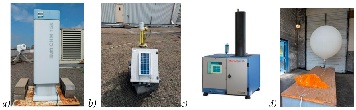
Figure 2.
Ceilometer vertical profiles of attenuated backscatter coefficients in July 2020.
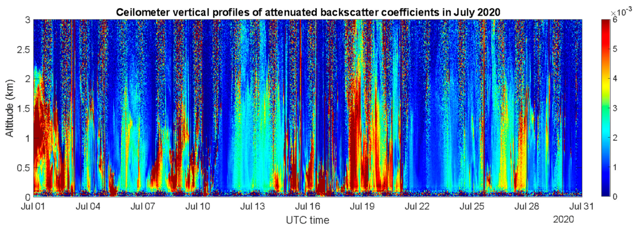
Figure 3.
Ceilometer attenuated Backscatter coefficients and aerosol Extinction Coefficient Vertical Profiles on a) June 10th, 2020; b) June 22nd, 2020, c) July 27th, 2020.
Figure 3.
Ceilometer attenuated Backscatter coefficients and aerosol Extinction Coefficient Vertical Profiles on a) June 10th, 2020; b) June 22nd, 2020, c) July 27th, 2020.
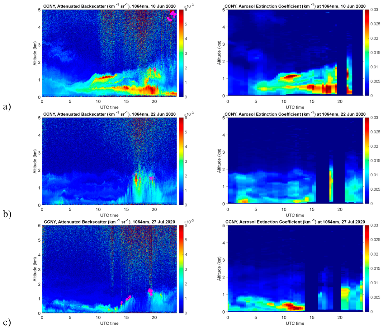
Figure 4.
Ceilometer attenuated Backscatter coefficient and aerosol Extinction Coefficient Vertical Profiles on a) June 1st, 2023; b) July 06th, 2023; c) July 22nd, 2023.
Figure 4.
Ceilometer attenuated Backscatter coefficient and aerosol Extinction Coefficient Vertical Profiles on a) June 1st, 2023; b) July 06th, 2023; c) July 22nd, 2023.
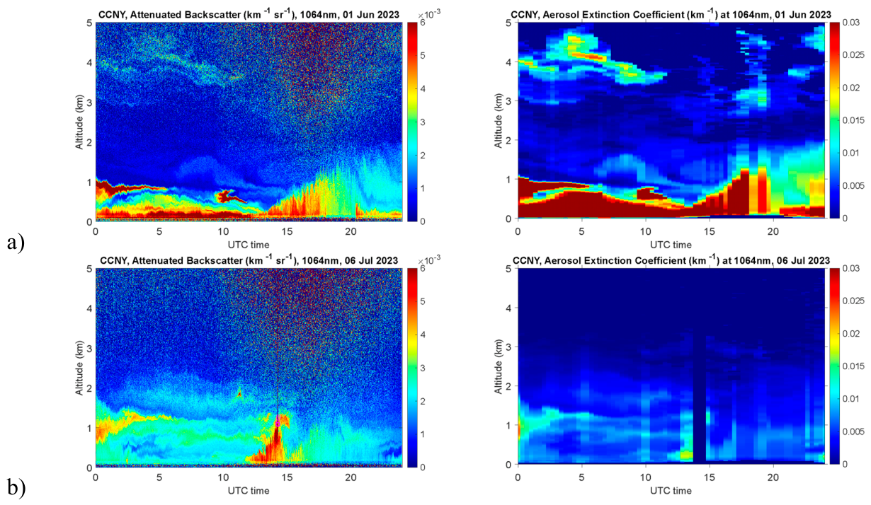
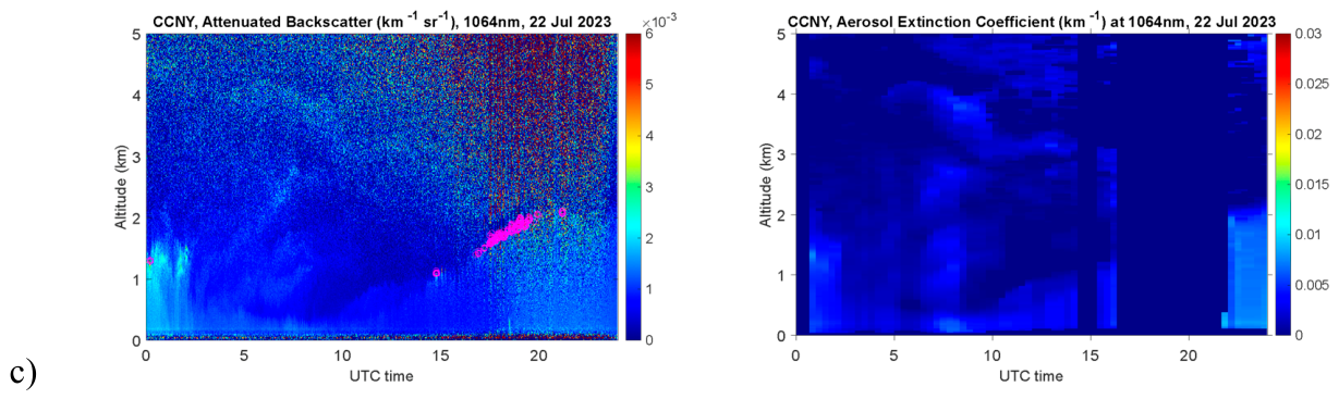
Figure 5.
LIDAR Retrieved AOD within the PBL only, 1064nm, CCNY.
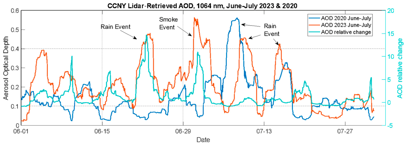
Figure 6.
Attenuated Backscatter (km−1 sr−1), 1064 nm, CCNY. a) 07 Jun 2023. b) 22 Jun 2023.
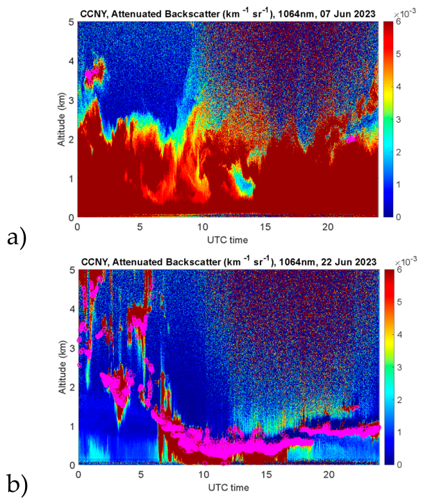
Figure 7.
AOD at 1020 nm retrieved by the CIMEL sunphotometer at CCNY for the periods. June-July 2020 and June-July 2023.
Figure 7.
AOD at 1020 nm retrieved by the CIMEL sunphotometer at CCNY for the periods. June-July 2020 and June-July 2023.
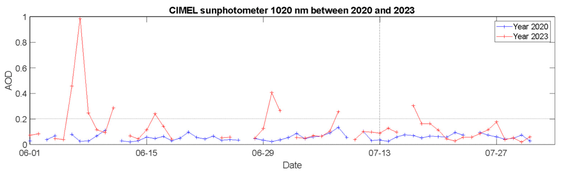
Figure 8.
HYSPLIT Trajectory, backward trajectories for 3 days. a) 07 Jun 2023. b) 22 Jun 2023.
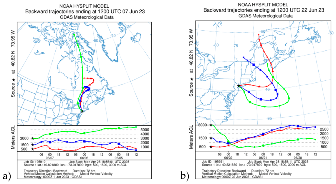
Figure 9.
Comparison of PM2.5 Concentration.
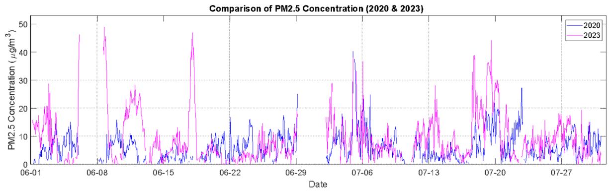
Figure 10.
Comparison of PM2.5 Concentration to Attenuated Backscatter with highlighted weekends. a) June-July 2020 and b) June-July 2023.
Figure 10.
Comparison of PM2.5 Concentration to Attenuated Backscatter with highlighted weekends. a) June-July 2020 and b) June-July 2023.
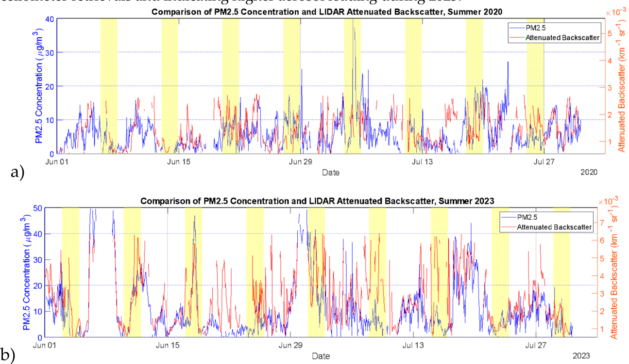
Figure 11.
Correlation between LIDAR Attenuated Backscatter and PM2.5.
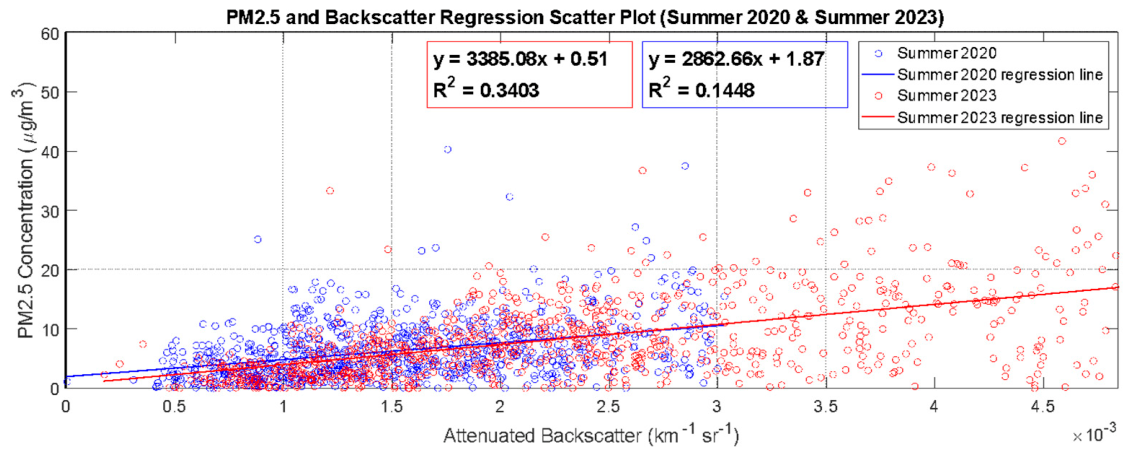
Figure 12.
AOD and PM 2.5 Relative change based on daily means between 2020 and 2023.
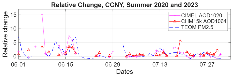
Figure 13.
Statistical analysis of the AOD and PM 2.5 distribution for the summers during pandemic (2020) and post pandemic (2023) period.
Figure 13.
Statistical analysis of the AOD and PM 2.5 distribution for the summers during pandemic (2020) and post pandemic (2023) period.
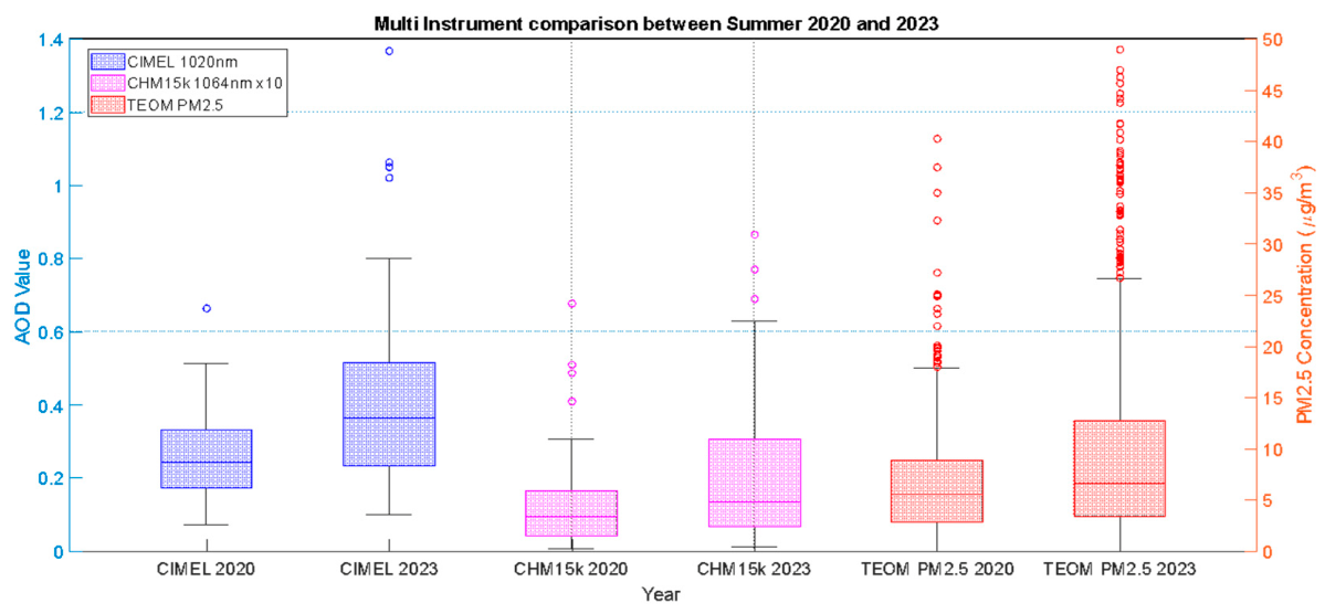

Table 1.
Statistical analysis of the AOD retrievals with CIMEL sunphotometer and Ceilometer LIDAR CHM15k. (smoke days were removed from the analysis).
Table 1.
Statistical analysis of the AOD retrievals with CIMEL sunphotometer and Ceilometer LIDAR CHM15k. (smoke days were removed from the analysis).
| Statistics | CIMEL 2020 | CIMEL 2023 | CHM15k 2020 | CHM15k 2023 | TEOM 2020 | TEOM 2023 |
| N | 50.000 | 44.000 | 53.000 | 54.000 | 1136.000 | 1147.000 |
| Mean | 0.257 | 0.441 | 0.132 | 0.212 | 6.392 | 9.240 |
| Median | 0.244 | 0.365 | 0.094 | 0.135 | 5.500 | 6.600 |
| Q1 | 0.172 | 0.232 | 0.041 | 0.068 | 2.800 | 3.400 |
| Q3 | 0.331 | 0.515 | 0.165 | 0.306 | 8.850 | 12.700 |
| IQR | 0.158 | 0.283 | 0.124 | 0.238 | 6.050 | 9.300 |
| WhiskerLow | 0.072 | 0.101 | 0.007 | 0.012 | 0.000 | 0.000 |
| WhiskerHigh | 0.512 | 0.801 | 0.305 | 0.628 | 17.900 | 26.600 |
| Min | 0.072 | 0.101 | 0.007 | 0.012 | 0.000 | 0.000 |
| Max | 0.664 | 1.368 | 0.678 | 0.866 | 40.300 | 49.000 |
| Std | 0.115 | 0.279 | 0.134 | 0.203 | 4.846 | 8.475 |
| OutlierCount | 1.000 | 4.000 | 4.000 | 3.000 | 25.000 | 56.000 |
Disclaimer/Publisher’s Note: The statements, opinions and data contained in all publications are solely those of the individual author(s) and contributor(s) and not of MDPI and/or the editor(s). MDPI and/or the editor(s) disclaim responsibility for any injury to people or property resulting from any ideas, methods, instructions or products referred to in the content. |
© 2026 by the authors. Licensee MDPI, Basel, Switzerland. This article is an open access article distributed under the terms and conditions of the Creative Commons Attribution (CC BY) license.
Copyright: This open access article is published under a Creative Commons CC BY 4.0 license, which permit the free download, distribution, and reuse, provided that the author and preprint are cited in any reuse.