

Submitted:
23 September 2026
Posted:
23 September 2026
You are already at the latest version
Abstract
An automatic discrimination of in-situ vitrinite on polished plugs by means of Raman spectroscopy is here proposed on a set of Mesozoic-Cenozoic samples from a well drilled in the Norwegian Sea, offshore mainland Norway. Publish Rock-Eval Pyrolysis predominantly indicates a Type III kerogen, with hydrogen enrichment in specific intervals probably due to organic mud additives used during drilling. In the same publish dataset, organic petrographic analyses show the coexistence of indigenous alongside reworked vitrinite and inertinite macerals. Thermal maturity derived from the reflectance of the indigenous vitrinite show a regular downward increase ranging approximately from 0.35% to 1.4%. Raman spectroscopic analyses have been performed on: 1) specific macerals optically recognized and 2) by high-resolution Raman mapping of small surface where different (i.e. vitrinite and inertinite) macerals have been previously identified. Thermal maturity Raman parameters show downward increase similar to the reflectance ones, when considering indigenous vitrinite fragments. On the other hand, high standard deviation, due to both the presence of different macerals or contaminants, hampers a correct evaluation when a Raman-mapped area is considered. Such a limitation is overcome by applying Mixed Gaussian Model automatic clustering that allows the discrimination of different organic material and the identification of the in-situ vitrinite by looking at the cluster distribution along the section. This work demonstrates how machine learning techniques applied to samples from drill cuttings can effectively reduce uncertainties in thermal maturity assessments.
Keywords:
dispersed organic matter
; Raman spectroscopy
; machine learning
; vitrinite reflectance
; Gaussian Mixture Model
1. Introduction
Automation can help energy producers to better compete in global markets and has advanced in many sectors of the oil and gas industry. Many exploration steps have already benefited from the application of data mining and machine learning techniques (Brackenridge et al., 2022). Despite this, other processes are still linked to classical analytical techniques that generally require time-consuming analyses, sample preparation and expert user interpretation. One such step is the assessment of thermal maturity by analysing the organic matter (OM) dispersed in sediments. OM derives mostly from the diagenetic alteration of the remains of organisms incorporated in sedimentary rocks during progressive burial. The residue left after the generation and expulsion of hydrocarbons becomes more enriched in carbon and rearranges into more condensed compounds, via the so-called aromatisation process, as temperature increases.
Vitrinite reflectance is generally considered a highly reliable and reproducible tool for dispersed OM thermal maturity assessment (e.g., [1,2,3]; among others), although it is semiquantitative, time-consuming and strongly dependent on the operator’s skill [4,5,6,7]. In this context, Raman spectroscopy has recently received attention as a tool to evaluate the thermal maturity of organic matter in source rocks to complement and enhance the traditional approaches (see [8,9] as the most recent reviews).
However, the limitations of Raman spectroscopy are still linked to the correct identification of organic facies [10]. In order to overcome this issue, recent studies have demonstrated that the combination of Principal Component Analysis (PCA) and supervised or unsupervised machine learning of OM Raman spectra can identify different organofacies with high precision [11,12] reducing the reliance on the aforementioned traditional organic petrographic and its limitations.
In this work, we aim to extend the use of machine learning techniques to map portion of petrographic plugs and to verify whether the indigenous organic matter can be automatically identified for thermal maturity assessment. To do this, geochemical and petrographic analyses were used to assess the thermal maturity of a well drilled in the Norwegian Sea, offshore mainland Norway (Figure 1a), and these were then compared with Raman spectroscopy outcomes.
2. Materials and Methods
2.1. Geological Setting and Well Stratigraphy
The study is located in the mid-Norwegian continental margin that extends between the North Sea to the SW and the Barents Sea to the NE (Figure 1). The S1 well was drilled in the Norwegian Sea in the so-called Sklinna High, located in the Halten/Dønna terraces between the Trøndelag Platform and the Møre Basin Mid(Figure 1). The map of Figure 1 shows the present--day structural configuration of the area that is still an inheritance of the Mesozoic extensional tectonics.
The study area was located at a tectonic boundary during the Caledonian orogeny, and, since Devonian times, has been subjected to recurring phases of extension. The main extensional phases can be observed in the S1 well stratigraphy (Figure 2), which reaches up to a TVD (Treu Vertical Distance) of 4492 m with the oldest recovered rocks dating to the Triassic.
The transition from the Grey to the Red beds is a typical Norian shift from coastal plain deposits under humid conditions to continental fluvial to coastal plain sedimentation [14]. Late Triassic Red Beds are cut by an unconformity upon which the Lower Cretaceous shales of the Lange Fm. directly lie (Figure 2). The Jurassic record is probably low due to the well’s location on a structural high at that time. In addition, the ridge area experienced erosion due to ridge-flank uplift as a consequence of the Jurassic rifting [15]. Subsidence continued throughout the entire Cretaceous and into the Paleocene and is recorded by the fine-grained marine sediments of the Crome Knoll and Shetland groups (Figure 2). The shaly Tang and Tare fms. of the Rogaland Group record the Paleocene-Eocene rifting phases following continental breakup and are overlain by the Eocene to early Miocene post-rift sandy and silty shales of the Brygge Fm. [13]. The top of the S1 well comprises about 500m of lower Miocene to upper Pleistocene marine sediments of the Kai Fm. (Figure 2).
2.2. Sample Preparation and Published Data Collection
Analysed samples in the study area derived from cuttings recovered during drilling. The samples were washed using a Soxlet apparatus to reduce the amount of organic contaminants from drilling mud. After that, polished plugs were prepared according to standardised procedures described in [16]. Samples were ground in a mortar and were embedded in an epoxy resin block (Serifix resin and hardener with a 1:20 ratio)
Samples were polished using an automated polishing system (Struers Labopol 5) with 250, 500 and 1000 grit carborundum paper and isopropanol lubricant. After washing the samples to remove debris, three polishing laps were used with alumina powders of decreasing grain size (1.00 and 0.30 µm), with the samples polished for a few minutes on each (Figure 4b). The use of 0.10 µm alumina was avoided, as it has been observed to slightly affect the Raman signal [17].
Publish geochemical data, including Rock-Eval Pyrolysis and vitrinite reflectance were collected from the website of the Norwegian Offshore Directorate at https://factpages.sodir.no/pbl/geochemical_pdfs/4762_1.pdf.
2.3. Raman Spectroscopy
Raman spectroscopy analyses were carried at the Raman Laboratory of the School of Geosciences at the University of Aberdeen. A Renishaw inVia Reflex Raman spectrometer was used, with a backscattering geometry in the range of 700– 2300 cm−1 (first-order Raman spectrum), a 2400 l/mm spectrometer grating and a CCD detector under a maximum of ×100 objective magnification (numerical aperture of the lens (NA) of 0.90). The Slit opening was set to 65um with a CCD area of approximately 10 pixels (80% of the total signal height hitting the CCD chip). The confocal hole was set to 200 μm. A 514.5 nm diode laser was used for excitation with an output of 50mW. Optical filters (1%) were used to adjust the laser power at the sample to less than 0.5 mW. The Raman backscattering was recorded using an integration time of 20 s and three repetitions per measurement. The Raman system was calibrated against the 520.7 cm−1 band of silica.
Raman deconvolution used a two-Lorentzian-band fitting performed using a modified version of the PeakFit program designed by [18,19]. This simplified method allows for the evaluation of basic Raman parameters avoiding errors derived from complex multiple fitting. A quadratic baseline was subtracted to correct highly fluorescing spectra with control points between 750 and 850 cm−1 and between 1880 and 1920 cm−1.
2.4. Unsupervised Clustering
Spike removal and normalisation relative to the mean intensities of the Raman spectra were performed as pre-processing steps before Principal Component Analysis (PCA) for dimensionality reduction and clustering analysis.
PCA was performed using the intensities of each spectrum (y-axis of the matrix) since the Raman shift (cm−1) values (x-axis) are the same in all spectra. PCA is a conventional dimensionality reduction technique that projects a multivariate (or high-dimensional) dataset into a lower-dimensional coordinate system that captures the maximum amount of variation in the dataset, ensuring minimal information loss [20]. Once the whole dataset has been reduced, a representative number of components (two in this work) was selected to proceed with the clustering analysis.
Clustering, also known as cluster analysis, aims to identify natural groupings or clusters within multidimensional data based on a chosen measure of “similarity” (e.g., Euclidean distance, probability distribution, etc.), so that data items within a cluster are very similar to each other but dissimilar to data items in other groups.
Gaussian Mixture Modeling (GMM) is a probabilistic model-based clustering method based on finite mixtures that provides an example of a “soft” clustering approach. In a mixture, clusters are represented by a set of probability distributions (e.g., Gaussian distributions [21]). A GMM can be represented as the weighted sum of a number of Gaussian component densities (i.e., the number of clusters). Each Gaussian in the mixture (i.e., a cluster) is characterised by its mean, covariance, and weight. The goal of GMM is to iteratively find the best combination of these parameters to define a number of clusters. GMM is particularly useful since it allows for the clustering of complicated geometrical shapes by combining the number of clusters (K) and the covariance matrix (Σj), which defines the cluster's geometry (shape and orientation). Both the optimal (K) and Σj are calculated by applying the Bayesian Information Criterion (BIC, [22]). The covariance matrix can be: 1) A full covariance matrix that can be independently oriented in any direction; 2) a diagonal matrix type where the clusters are forced to be oriented along the coordinate axes. Both types of covariance matrices can have an unshared structure where each Gaussian distribution can independently differ in size and orientation, or a shared structure where all distributions are of the same size and orientation [23] . For a detailed explanation of GMM and BIC see [12] and references therein.
The workflow used in this work that include PCA dimensionality reduction, GMM clustering and an automatic fitting to derive Raman spectra is shown in Figure 3.
3. Results
3.1. Description of Published Geochemical and Optical Data
As part of the well completion report when the S1 well was drilled, TOC and Rock-Eval Pyrolysis were measured between 3500 and 4500 m of depth. From now onrwards, TOC will be express as the percentage of organic carbon in the total weight of the rock and HI as mgHC/g TOC. Data indicate that TOC remains relatively constant within a range of 0.5% to about 3%, with most of the samples between 1% and 2%. Some outliers with TOC content higher than 4% exist and the maximum value is of 20% at about 3800 m of depth. Tmax shows valuesmainly rangescomprised between 430 and 440ºC with no evident trend with depth, while HI data decrease from about 500 to 200 between 3500-3800 m of depth and then increase again toward the bottom of the well showing maximum values of more than 600 in samples deeper than 4200 m (Figure 4).
The inverse HI trend and the very high values at the bottom of the well can hardly be justified by geological evidence or by OM composition (as will be shown by optical analyses in the following paragraphs) and have thus been interpreted as resulting from the presence of Gilsonite-rich contamination from the organic mud additives.
Due to the abnormally high HI values, especially at the bottom of the well, Tmax data are not reliable, and this can lead to thermal maturity underestimation as well as incorrect interpretation of the hydrocarbon potential of the source rocks. This is evidenced in the pseudo-Van Krevelen diagram of Figure 5 where the deepest samples fall in the thermally immature range of a Type I kerogen.
Pertaining to the same database, optical analyses under transmitted light performed indicate a predominance of continentally derived OM and subordinately phytoplankton and some AOM in only 4 samples (Table 1). Yellow fluorescence from OM was observed in the top 3500 m of depth, and dull fluoresce between 3500 and 4000, while below this depth no fluorescence has been observed.
Yellow and dull fluorescence in the shallowest samples correspond to Thermal Alteration Index (TAI) values between 1.2 and 2, while its disappearance corresponds to a TAI shift to 2.5-2.7 up to more than 3 in sample 4415 (Table 1).
Reflected light analyses show an abundance of continentally derived OM with many reworked vitrinite fragments (Table 1 and Figure 6a), which are sometimes more abundant than the indigenous vitrinite population. Some fusinite and semi-fusinite macerals have also been observed, with respective reflectance values that can be either higher or lower than those of the indigenous vitrinite (Figure 6b). The number of measured fragments for indigenous vitrinite are generally high enough for thermal maturity estimation (Table 1).
3.3. Raman Spectroscopy
3.3.1. Raman Analyses on Polished Plugs
Analyses on polished plugs conducted using the optical system mounted on the Raman microscope outline the limits in recognising macerals when observed under air immersion. Figure 7a shows an example of a polished plug and how macerals appear under oil (for Ro% measurements) and air immersion (for Raman measurements). During optical observation with the Raman instrument, vitrinite can hardly be recognised in the very immature samples since the colour contrast against the surrounding matrix is very low (depth 2480 in Figure 7b). However, some little fragments can be recognised, or some OM can be found around framboidal pyrite (depth 4500m in Figure 7b).
At higher maturity levels, vitrinite fragments are more easily recognisable due to their brighter surfaces. Inertinite fragments, on the other hand, can be recognised due to their shape or the presence of evident cellular structure as in the case of fusinite (Figure 7b), while detrital OM often shows typical spectra of graphitic carbon and can thus be easily discarded.
Figure 8 shows the trends of two Raman parameters (i.e. D-G distance and FWHM-G) measured on vitrinite fragments at different depths and compared with the Ro%-defined thermal maturity trend across the well. The two parameters show a continuous trend up to the bottom of the well. The highest standard deviations were found for the shallowest samples probably due to the difficulties in vitrinite recognition at the lowest maturity levels.
3.3.2. Surface Mapping and GMM Clustering on Polished Plugs
Given the low spatial resolution of Raman mapping, mapping the entire surface of a plug is too computationally intensive and time-consuming. For this reason, small areas were mapped and then all data from these areas were processed together, assuming they are representative of a portion of the sample as large as possible. Figure 8 is an example of an area mapped by Raman. The mapping is a function of the intensity of the G band with respect to the baseline and was generated with the Renishaw software. Colors in the map serve only to illustrate the variability of the Raman spectra across the mapped area.
In the upper-left photograph part of Figure 9, some macerals can be recognised by their shapes and brighter colours relative to the background. These have been interpreted as in-situ vitrinite in the centre and inertinite on both sides. The Raman map shown lower left part of Figure 9 associates the less mature spectra with the brightest colours and the more mature spectra with the darkest. The map thus confirms the optical interpretation showing a black colour to the left and to the right of the mapped window and dark brown in the centre. Moreover, traces of carbon have been found throughout theentire matrix (see Discussion below).
Combining the maps for each sample results in a very high number of spectra.
Table 2 shows the total number of spectra acquired for each sample and the spectra used for thermal maturity assessment after GMM clustering (see Discussion below). The average Raman parameters for all these spectra collected for each sample is shown in Figure 10.
Figure 10 outlines a weak trends and very high standard deviations. Both observations suggest that while in-situ OM may be a prominent component of the surfaces mapped by Raman, but a significant component of reworked OM or other organofacies (e.g. AOM, palynomorphs or even contaminants) is present, increasing the uncertainty of each measured value.
To reduce this uncertainty, the GMM clustering serves as a valid tool, as suggested in the previous sections. Figure 11 shows an example of PCA dimensionality reduction and GMM clustering for the sample at 3790 m of depth (GMM outputs for all samples can be found in the Supplementary Materials). After spectra normalisation (Figure 11 a), the robustness of the PCA dimensionality reduction was validated by the percentage of explained variance (Figure 11 b). For our dataset, more than 90% of the variance is explained by the first two or three first PCs. After plotting the first and second PCs on a score plot (Figure 11 c) the GMM clustering was applied (Figure 11 d). The first cluster is generally characterised by a narrow oval extended along the y-axis (i.e. PC2) while the second and third clusters show more variance along PC1.
4. Discussion
4.1. Source Rock Quality and Organofacies Content
The source rock quality in the well is generally poor considering TOC values between 1 and 2%. Tmax and HI, on the other hand, show anomalous trends that slightly increase moving toward the highest maturities (i.e. after 4200 m of depth, Figure 4). This increase is not justified by the organofacies content in Table 1 that outline AOM and Marine phytoplankton (MPH) values together generally account for around 30%. Usually, such low content of marine-derived organic matter is usually associated with HI values typical of a type III kerogen, thus below 200-300 mg/gTOC.
Considering thermal maturity higher than 1% and the absence of fluorescence (Table 1) at the bottom of the well, the classification of a type II kerogen at the onset of the oil window as shown by the pseudo Van-Krevelen diagram in Figure 3 is highly suspicious, as are the Tmax maturities depicted for samples deeper than 3500m.
The anomalous HI and Tmax data may be explained by the presence of gilsonite, which is a low-maturity solid bitumen found in drilling muds, which likely also influences the observed TOC values. Gilsonite could have also, potentially, affected reflectance measurements. However, the increase in indigenous vitrinite reflectance with depth (Figure 6) is consistent with the depth increase and suggests that contamination has been avoided.
Organic petrography under reflected light also indicates the diffuse presence of a second family of reworked vitrinite together with fusinite and semifusinite. This latter showing lower reflectance values than in-situ vitrinite at greater depths.
4.2. Raman Spectroscopy Under Air Immersion Microscopy
Petrographic observation has proven to be useful on coals [24,25] or in source rocks with a high TOC [11], however in the low-TOC samples here may present a limitation. This is true in particular at the lowest maturities where the reflectance of vitrinite under air immersion can be similar to that of the surrounding matrix. Despite this, some vitrinite-like fragments have been recognised even at the lowest maturities (Figure 6b) and the calculated parameters for the supposedly indigenous vitrinite show a trend with depth for the D-G distance and the width of the G band (Figure 8) suggesting we are dealing with indigenous organic matter. The D-G values show an increase from about 215 cm-1 at the top to about 240 cm-1 st the bottom of the well (Figure 8) even if with some outlier or samples with very high standard deviation. The width of the G band shows a better inverse trend from about 60 cm-1 to barely 45 cm-1 moving toward the bottom. These values can be compared with the general trends depicted by [8] in one of the most complete reviews on Raman spectroscopy applied to kerogen. The general trend presented by [8] suggests values of both parameters correspond to the early level of maturation, roughly between 0.3/0.4% and 1% vitrinite reflectance, thus confirming the thermal maturity derived from vitrinite reflectance.
It is worth noting that spectra with very high fluorescence that overwhelms most of the signal have been encountered at every depth and have been interpreted to belong to the mud additive gilsonite.
4.3. Unsupervised Clustering
The validity of unsupervised clustering for characterisation of different organofacies by means of their Raman spectra has been demonstrated by [12]. In this work, we take a step forward by applying it to the surface mapping on polished plugs. The maceral content of our samples is mainly characterised by a high content of terrestrially derived OM (i.e. vitrinite and inertinite) with a minor amount of hydrogen-rich OM such as AOM and marine phytoplankton (Table 1). The cluster shapes described in Figure 11 d resemble those found in [11,12] with the one of the first cluster being typical of highly fluorescing spectra. In the case of mapping is possible that most of the matrix, including the inorganic components, was recorded in this cluster. The extension of the second and third cluster along PC1, on the other hand, indicate a higher variation of the spectra in these two groups, which is consistent with the nature of the vitrinite and inertinite groups.
4.4. Automatic Maceral Discrimination
Understanding how to identify indigenous organic matter for thermal maturity assessment has been one of the main goals of coal geology [26]. For industrial applications, a spectroscopic mapping assisted by a machine learning approach for macerals or organofacies determination could avoid time-consuming/user-dependent analyses during the phases of exploration, reducing the uncertainties related to the maturity assessment. Here we are proposing a robust user-guided mapping approach that can be the first step toward a fully automated approach in the future.
Figure 12 shows the differences in Raman spectra over each analysed area that can be mapped by a simple analysis of the G band with respect to the baseline of the spectra (GMM results for all the samples can be found in the supplementary materials). With GMM we forced the method to summarize all of these differences into three main clusters. This has been chosen because previous works [11,12] have suggested that for macerals and organofacies descriptions by means of their Raman spectra the division into three main groups (i.e. AOM/liptinite, translucent phytoclasts/vitrinite and opaque phytoclasts/inertinite) is the best option. This is also confirmed by petrographic analyses shown in Table 1 and Figure 6.
Cluster analysis has found three main groups that can be divided and described easily by looking at the spectra fluorescence and D and G band properties (Figure 11):
- 1)
- Very high-fluorescing spectra almost without bands apart from a slight protuberance corresponding to the G band region (ca 1600 cm-1);
- 2)
- High-fluorescing spectra at shallow depth evolving into low-fluorescing spectra with well-defined D and G bands;
- 3)
- Low-fluorescing spectra with well-defined D and G bands.
GMM clustering used to determine three clusters points out that in most cases the in-situ materials can be located among the centred clusters of the score plot (Figure 12). In the clusters toward the higher PC1 values, usually reworked material of inertinites is found, sometimes with a high content of graphitic carbon, as shown for the deepest sample in Figure 12. The most surprising outcome of the clustering analyses is that the matrix is always characterised by a very slightly presence of (apparently) very immature carbon material as indicated by the clusters with the lowest PC1 values in Figure 12. These low maturity spectra have been supposed to represent the gilsonite mud additive.
After visual inspection, the group 1 and 3 spectra (respectively the one with lowest and highest PC1 values) show almost no differences with depth while the spectra of the central group, that is usually the second cluster (from left to right in Figure 12), evolves with depth. This is a first clue of a possible correlation with indigenous vitrinite.
If the spectra from mapping (Table 2) are deconvoluted all together, the resulting Raman parameters will show extremely high standard deviations (Figure 11). Even if is a slightly trend of the average values can be observed, the error is too high for any attempts to derive thermal maturity from these data. As noted in [11,12] one of the main aims of the clustering analyses for organic matter is to reduce the standard deviation when dealing with indigenous OM. This can be observed also in our dataset in Figure 13 where Raman parameters from the second clusters interpreted as indigenous vitrinite have been plotted against the range of error of the same parameters measured on the whole mapping dataset as in Figure 12 (dotted lines) and derived by means of petrographic analyses (grey shaded area). In the same figure, the trend and standard deviation range of Raman parameters measured on visually identified vitrinite are also plotted in translucent white colours.
Figure 13 thus suggests that the spectra identified by unsupervised clustering after Raman mapping significantly reduce the standard deviation and, in many cases, better approximate the means values to those calculated by optical observations, demonstrating the power of this method to improve thermal maturity assessment in complex samples.
4.5. Limitations and Future Work
The main limitations that future studied should address to explore the possibility of developing a fully automated method for indigenous organic matter discrimination and thermal maturity assessment can be outlined as:
- 1)
- Our mapping has thus far been done on very small areas whose size is still in the range of a few mm. To map a larger area or the entire surface of a plug, a dedicated instrument with an appropriate laser and the capacity to reduce the acquisition time would be needed;
- 2)
- Autofocusing will remain a challenge since macerals are still hardly recognizable under an optical microscope;
- 3)
- The standard deviation is still high for low maturity samples;
- 4)
- The cluster of in-situ vitrinite has been chosen by the operator while in the future this could also be part of an automatic routine.
5. Conclusions
Raman mapping to identify organic matter on polished petrographic plugs can be an alternative to classic organic petrography. However, the discrimination of in-situ vitrinite and the problem posed by the use of organic mud additives during drilling are still a challenge.
In this work we applied an automatic clustering to identify indigenous vitrinite from Raman mapping on small areas selected on the surface of petrographic plugs. Raman analyses on optically selected vitrinite shows an increase of thermal maturity Raman parameters with depth. On the other hand, all the spectra from Raman mapping show too high standard deviation to be used for thermal maturity assessment.
A GMM clustering of the Raman spectra of the mapped area indicate the organic material can be divided into three main clusters on a score plot. The central cluster seems to show a trend with depth, and this suggest a correspondence with in-situ vitrinite.
Our results show that this method can be successfully used to determine the indigenous thermal maturity trend of, even though some technical challenges still need to be addressed in future work.
Supplementary Materials
The following supporting information can be downloaded at the website of this paper posted on Preprints.org.
Author Contributions
Conceptualization, A.S., S.C., R.G., E.C. and F.T.; methodology, A.S., S.C., N.V.S.; software, A.S., N.V.S.; validation, A.S., E.G.R., D.M. and G.A.G.P.; formal analysis, A.S.; investigation, A.S:, S.C., E.G.R.,; resources, A.S., S.C., D.M., E.C., R.G. and F.T.; data curation, A.S., E.G.R., S.C., E.C.; writing—original draft preparation, A.S., S.C., E.C., R.G., F.T.; writing—review and editing, A.S., E.G.R., G.A.G.P., N.V.S. D.M., E.C., R.G., F.T.; visualization, A.S., G.A.G.P., E.C., R.G..; supervision, A.S., D.M., S.C.; project administration, A.S., D.M., S.C.; funding acquisition, A.S., S.C., R.G., F.T. All authors have read and agreed to the published version of the manuscript.
Funding
The research of the first author AS is funded by the Ramón y Cajal Program (RYC- 2022) nº RYC2022-036094-I MCIN/AEI/10.13039501100011033, funded by the Spanish Ministry of Science and Innovation and cofounded by the European Union (FSE+).The research was supported by GeoTech division of GEOLOG S.r.l. and Vår Energi ASA.
Data Availability Statement
Result of GMM clustering are provided in the supplementary materials.
Acknowledgments
GeoTech division of GEOLOG S.r.l. and Vår Energi ASA are acknowledged to support this research.
Conflicts of Interest
The authors declare no conflicts of interest.
References
- McCartney, J.T.; Teichmüller, M. Classification of Coals According to Degree of Coalification by Reflectance of the Vitrinite Component. Fuel 1972, 51, 64–68.
- Senftle, J.T.; Landis, C.R. Vitrinite Reflectance as a Tool to Assess Thermal Maturity. 1991.
- Tissot, B.P.; Pelet, R.; Ungerer, P.H. Thermal History of Sedimentary Basins, Maturation Indices, and Kinetics of Oil and Gas Generation. Am. Assoc. Pet. Geol. Bull. 1987, 71, 1445–1466.
- Schito, A.; Corrado, S.; Aldega, L.; Grigo, D. Overcoming Pitfalls of Vitrinite Reflectance Measurements in the Assessment of Thermal Maturity: The Case History of the Lower Congo Basin. Mar. Pet. Geol. 2016, 74, 59–70.
- Corrado, S.; Schito, A.; Romano, C.; Grigo, D.; Poe, B.T.; Aldega, L.; Caricchi, C.; Di Paolo, L.; Zattin, M. An Integrated Platform for Thermal Maturity Assessment of Polyphase, Long-Lasting Sedimentary Basins, from Classical to Brand-New Thermal Parameters and Models: An Example from the on-Shore Baltic Basin (Poland). Mar. Pet. Geol. 2020, 122, 104547.
- Nirrengarten, M.; Mohn, G.; Schito, A.; Corrado, S.; Gutiérrez-García, L.; Bowden, S.A.; Despinois, F. The Thermal Imprint of Continental Breakup during the Formation of the South China Sea. Earth Planet. Sci. Lett. 2020, 531, 115972.
- Sorci, A.; Cirilli, S.; Clayton, G.; Corrado, S.; Hints, O.; Goodhue, R.; Schito, A.; Spina, A. Palynomorph Optical Analyses for Thermal Maturity Assessment of Upper Ordovician (Katian-Hirnantian) Rocks from Southern Estonia. Mar. Pet. Geol. 2020, 120, 104574.
- Henry, D.G.; Jarvis, I.; Gillmore, G.; Stephenson, M. Raman Spectroscopy as a Tool to Determine the Thermal Maturity of Organic Matter: Application to Sedimentary, Metamorphic and Structural Geology. Earth. Sci. Rev. 2019, 198, 102936.
- Schito, A.; Muirhead, D.K.; Parnell, J. Towards a Kerogen-to-Graphite Kinetic Model by Means of Raman Spectroscopy. Earth. Sci. Rev. 2023, 237, 104292.
- Schito, A.; Spina, A.; Corrado, S.; Cirilli, S.; Romano, C. Comparing Optical and Raman Spectroscopic Investigations of Phytoclasts and Sporomorphs for Thermal Maturity Assessment: The Case Study of Hettangian Continental Facies in the Holy Cross Mts.(Central Poland). Mar. Pet. Geol. 2019, 104, 331–345.
- Schito, A.; Guedes, A.; Valentim, B.; Vergara Sassarini, N.A.; Corrado, S. A Predictive Model for Maceral Discrimination by Means of Raman Spectra on Dispersed Organic Matter: A Case Study from the Carpathian Fold-and-Thrust Belt (Ukraine). Geosciences (Basel). 2021, 11, 213.
- Sassarini, N.A.V.; Schito, A.; Gasparrini, M.; Michel, P.; Corrado, S. Automatic Organofacies Identification by Means of Machine Learning on Raman Spectra. Int. J. Coal Geol. 2023, 271, 104237.
- Færseth, R.B. The Deep Møre and Vøring Basins of the Norwegian Sea as Basement Highs Prior to Late Jurassic Rifting. 2021.
- Müller, R.; Ngstuen, J.P.; Eide, F.; Lie, H. Late Permian to Triassic Basin Infill History and Palaeogeography of the Mid-Norwegian Shelf—East Greenland Region. In Norwegian Petroleum Society Special Publications; Elsevier, 2005; Vol. 12, pp. 165–189 ISBN 0928-8937.
- Yielding, G.; Badley, M.E.; Roberts, A.M. The Structural Evolution of the Brent Province. Geological Society, London, Special Publications 1992, 61, 27–43.
- Bustin, R.M.; Barnes, M.A.; Barnes, W.C.; McIleareath, I.A.; Morrow, D.W. Determining Levels of Organic Diagenesis in Sediments and Fossil Fuels. Diagenesis, Geoscience Canada Reprint, 4th series 1990, 205–226.
- Lünsdorf, N.K. Geothermometry by Raman Spectroscopy of Dispersed Organic Matter. 2016.
- O’Haver, T. A Pragmatic Introduction to Signal Processing. University of Maryland at College Park 1997, 106.
- Schito, A.; Pensa, A.; Romano, C.; Corrado, S.; Vona, A.; Trolese, M.; Morgavi, D.; Giordano, G. Calibrating Carbonization Temperatures of Wood Fragments Embedded within Pyroclastic Density Currents through Raman Spectroscopy. Minerals 2022, 12, 203.
- Jolliffe, I.T. Principal Component Analysis; Springer, 2002;
- Everitt, B.S.; Hand, D.J. Mixtures of Normal Distributions. In Finite Mixture Distributions; Springer, 1981; pp. 25–57.
- Schwarz, G. Estimating the Dimension of a Model. The annals of statistics 1978, 461–464.
- Murphy, K.P. Machine Learning: A Probabilistic Perspective; MIT press, 2012; ISBN 0262304325.
- Guedes, A.; Valentim, B.; Prieto, A.C.; Rodrigues, S.; Noronha, F. Micro-Raman Spectroscopy of Collotelinite, Fusinite and Macrinite. Int. J. Coal Geol. 2010, 83, 415–422.
- Wilkins, R.W.T.; Boudou, R.; Sherwood, N.; Xiao, X. Thermal Maturity Evaluation from Inertinites by Raman Spectroscopy: The ‘RaMM’Technique. Int. J. Coal Geol. 2014, 128, 143–152.
- Suárez-Ruiz, I.; Flores, D.; Mendonça Filho, J.G.; Hackley, P.C. Review and Update of the Applications of Organic Petrology: Part 1, Geological Applications. Int. J. Coal Geol. 2012, 99, 54–112.
Figure 1.
Location of the study area (inset) and structural map of the Norwegian Sea. Modified after [13].
Figure 1.
Location of the study area (inset) and structural map of the Norwegian Sea. Modified after [13].
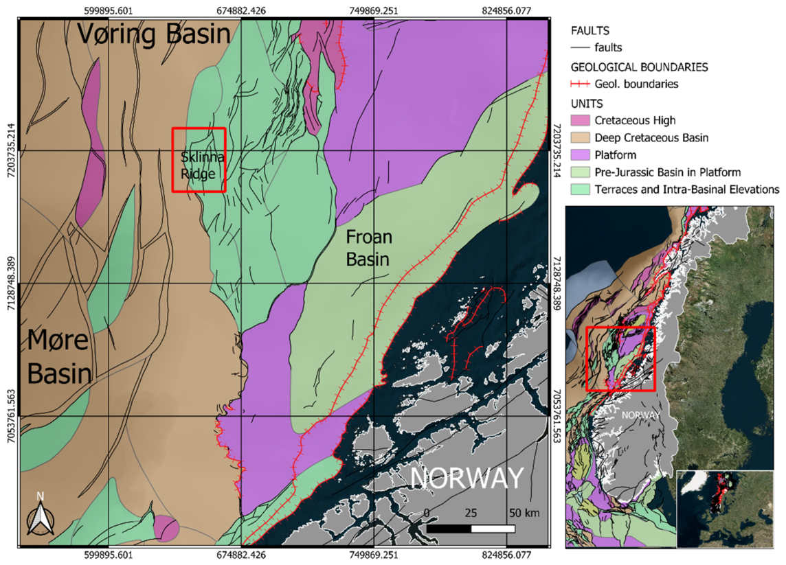
Figure 2.
S1 well stratigraphy showing ages, stratigraphic groups, depth (m) and lithology of the main drilled formations.
Figure 2.
S1 well stratigraphy showing ages, stratigraphic groups, depth (m) and lithology of the main drilled formations.
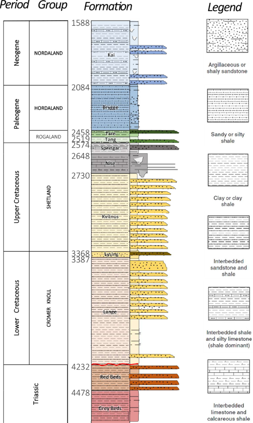
Figure 3.
Workflow of the unsupervised learning routine from raw Raman spectra for evaluation up to deconvolution to obtain thermal maturity Raman parameters.
Figure 3.
Workflow of the unsupervised learning routine from raw Raman spectra for evaluation up to deconvolution to obtain thermal maturity Raman parameters.
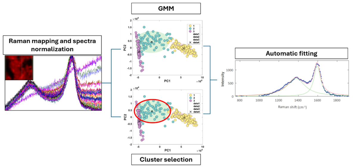
Figure 4.
TOC, Tmax and HI between 3500 and 4500 m of depth for the S1 well.
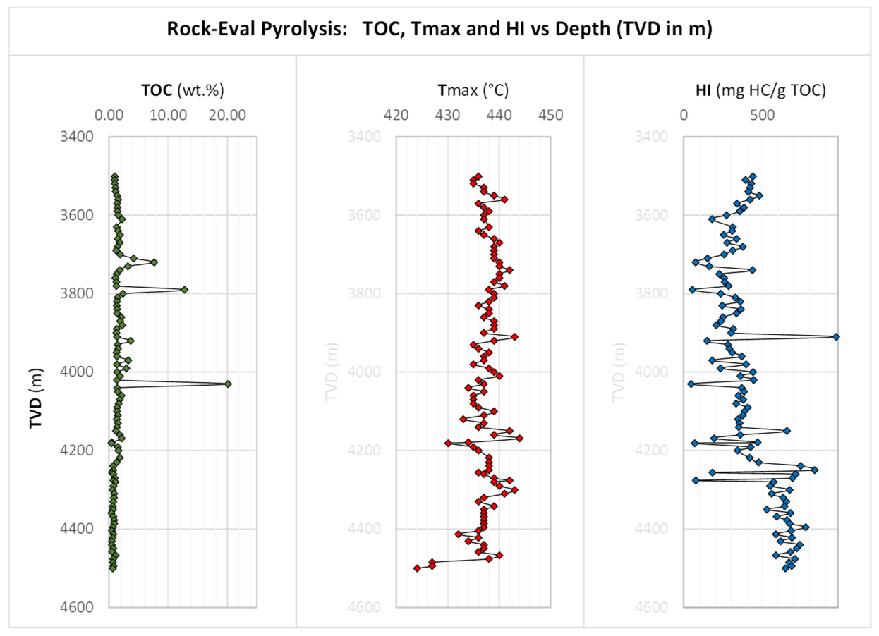
Figure 5.
Pseudo- Van Krevelen diagram for the S1 well.
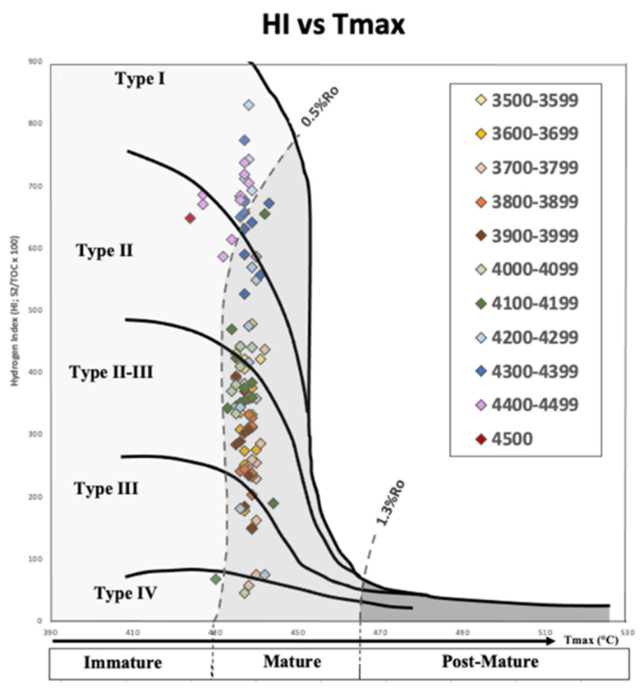
Figure 6.
a) Ro% maturity trend across the S1 well for both in-situ and reworked vitrinite and b,c,d) reflectance histograms showing average values for different macerals families at increasing depths. Data from https://factpages.sodir.no/pbl/geochemical_pdfs/4762_1.pdf.
Figure 6.
a) Ro% maturity trend across the S1 well for both in-situ and reworked vitrinite and b,c,d) reflectance histograms showing average values for different macerals families at increasing depths. Data from https://factpages.sodir.no/pbl/geochemical_pdfs/4762_1.pdf.
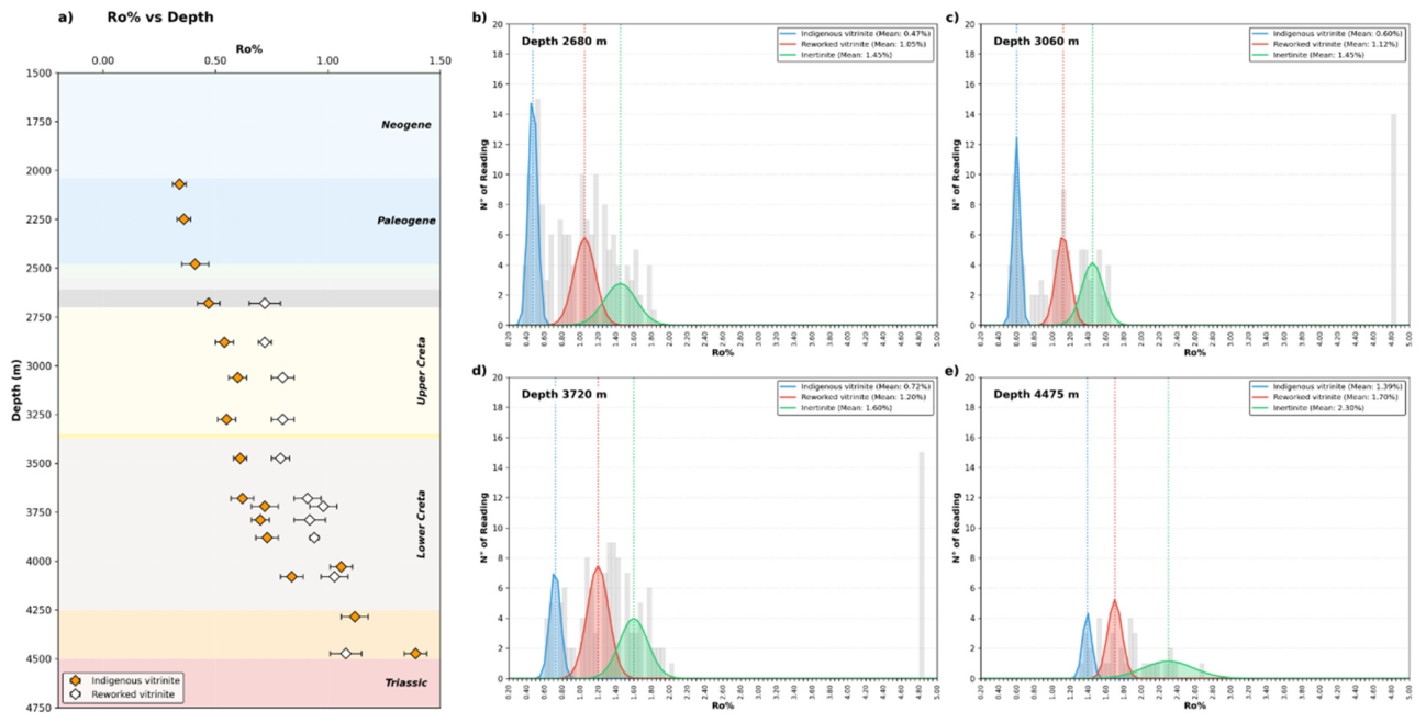
Figure 7.
a) above a polished plug and below how vitrinite appears under oil immersion in an organic petrography microscope or under air immersion during Raman analyses; b) examples of measured particles under Raman microscope and relative spectra.
Figure 7.
a) above a polished plug and below how vitrinite appears under oil immersion in an organic petrography microscope or under air immersion during Raman analyses; b) examples of measured particles under Raman microscope and relative spectra.
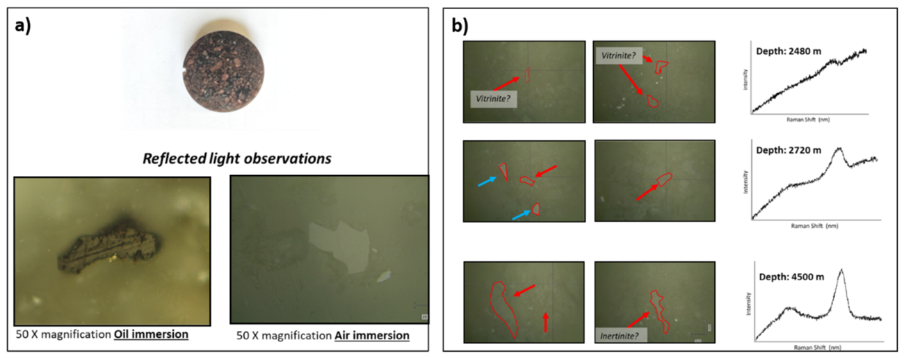
Figure 8.
a) Indigenous vitrinite reflectance across the well; b) D-G distance and c) width of the G band, measured on vitrinite evolution across the well.
Figure 8.
a) Indigenous vitrinite reflectance across the well; b) D-G distance and c) width of the G band, measured on vitrinite evolution across the well.
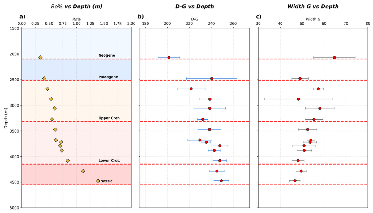
Figure 9.
An example of the Raman mapping and the meaning (in terms of spectra) of the colour bar in the legend.
Figure 9.
An example of the Raman mapping and the meaning (in terms of spectra) of the colour bar in the legend.
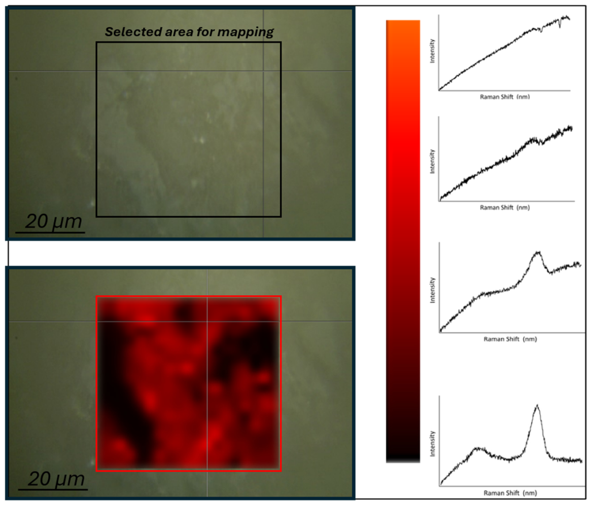
Figure 10.
D-G distance and G width parameters at different depths.
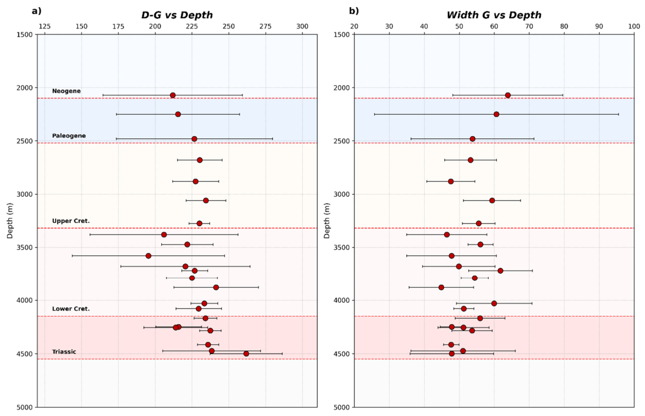
Figure 11.
Example of PCA and GMM results for spectra at 3790 m of depth. a) normalised spectra; b) percentage of explained value of the first 10 PCs; c) score plot after PCA; d) GMM clustering.
Figure 11.
Example of PCA and GMM results for spectra at 3790 m of depth. a) normalised spectra; b) percentage of explained value of the first 10 PCs; c) score plot after PCA; d) GMM clustering.
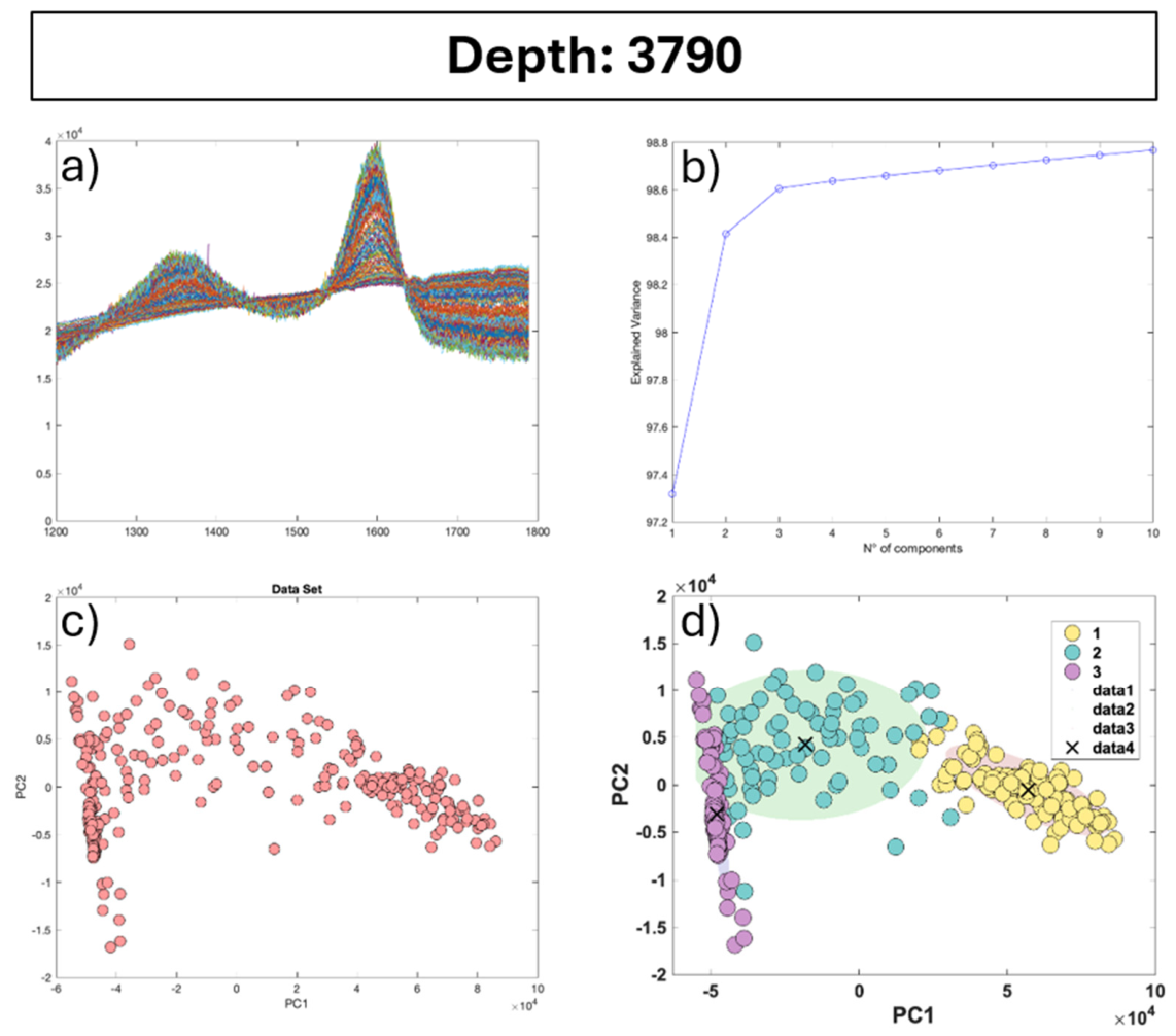
Figure 12.
Three examples of score plots and resulting average spectra at different depths across the well.
Figure 12.
Three examples of score plots and resulting average spectra at different depths across the well.
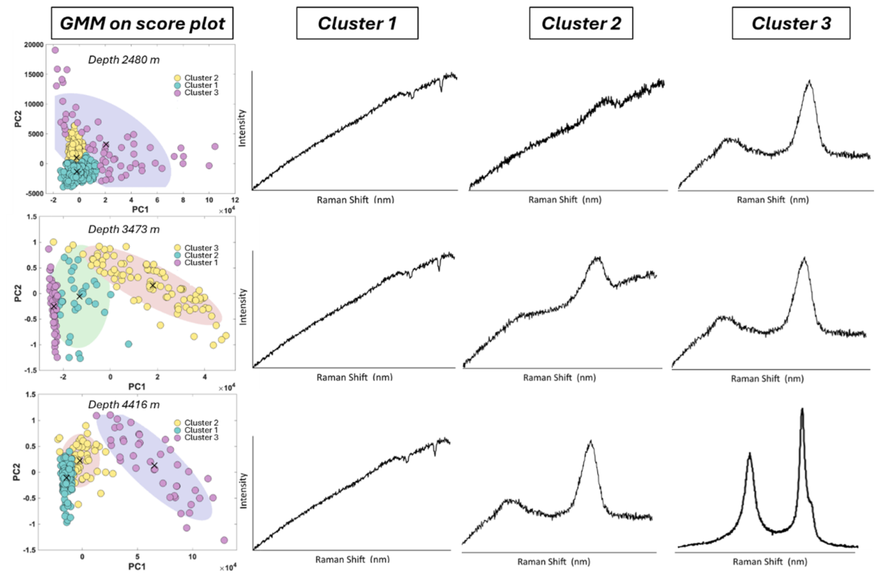
Figure 13.
D-G distance parameter after GMM (to the left) and compared with mean values (empty dots) and standard deviation (dotted line) before GMM. Grey shaded area is the standard deviation measured on in-situ vitrinite.
Figure 13.
D-G distance parameter after GMM (to the left) and compared with mean values (empty dots) and standard deviation (dotted line) before GMM. Grey shaded area is the standard deviation measured on in-situ vitrinite.
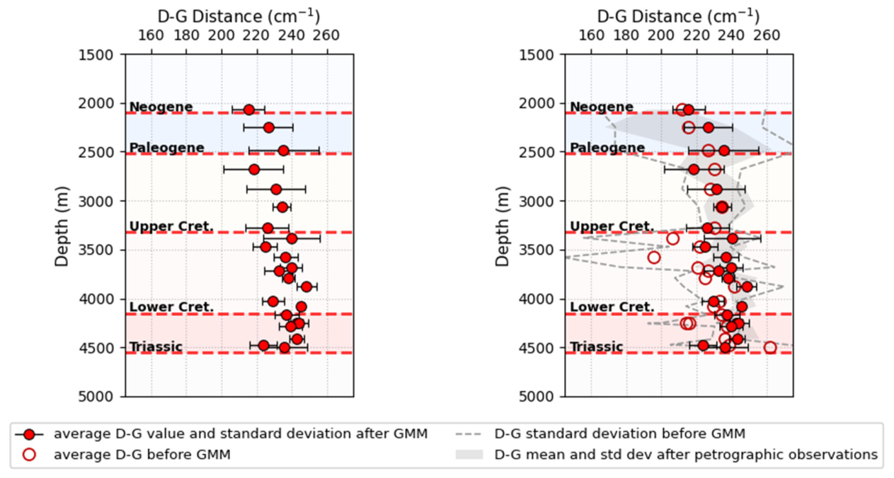

Table 1.
Organic facies and vitrinite reflectance assessment for the studied samples.
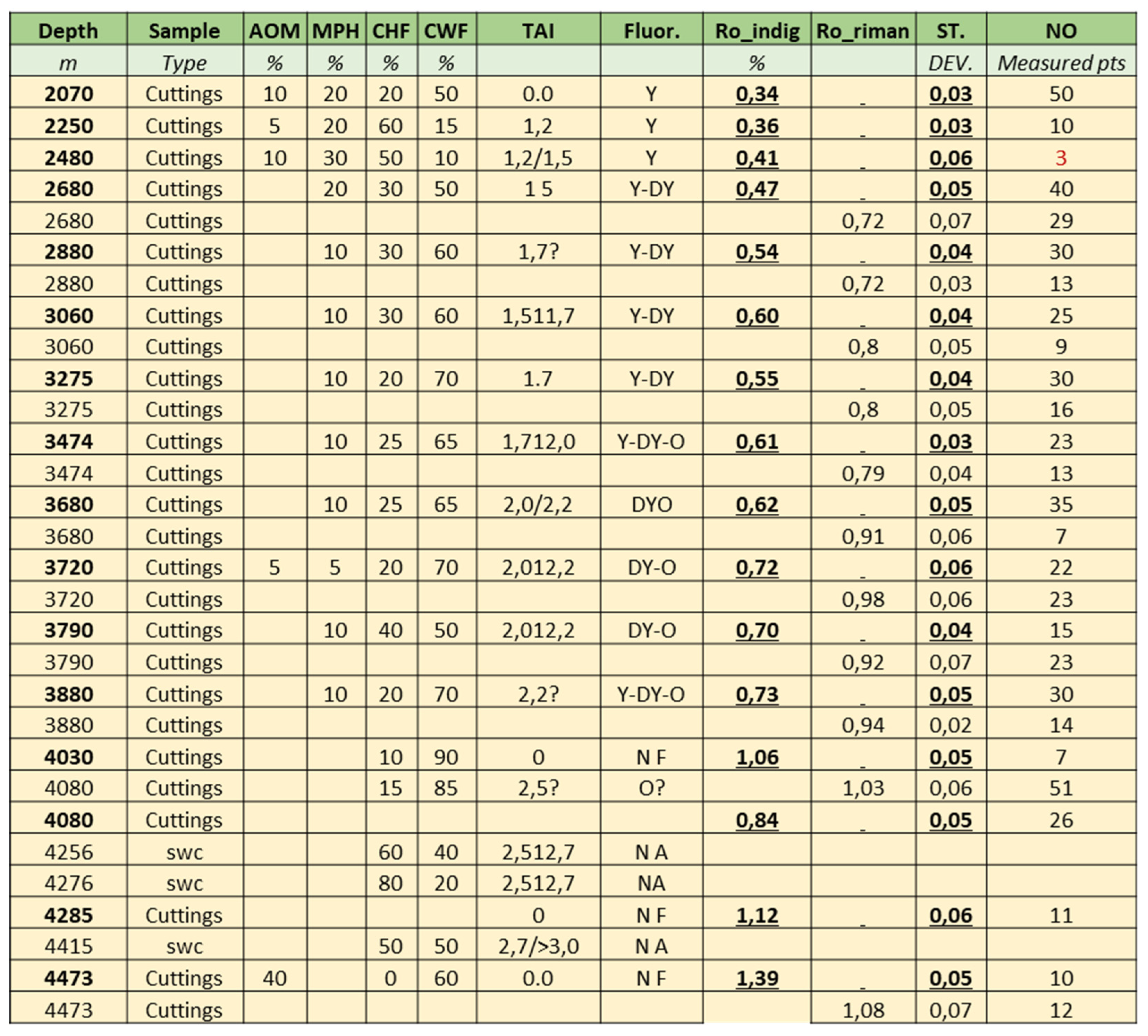 |
Table 2.
number of spectra obtained by summing mapping on each sample and number of spectra used for thermal maturity assessment after GMM.
Table 2.
number of spectra obtained by summing mapping on each sample and number of spectra used for thermal maturity assessment after GMM.
| Depth (m) | N° spectra | N°spectra after GMM |
| 2070 | 168 | 81 |
| 2250 | 808 | 354 |
| 2480 | 780 | 35 |
| 2680 | 193 | 71 |
| 2880 | 81 | 48 |
| 3060 | 244 | 36 |
| 3275 | 182 | 18 |
| 3380 | 572 | 18 |
| 3473 | 169 | 35 |
| 3580 | 450 | 25 |
| 3680 | 240 | 28 |
| 3720 | 280 | 168 |
| 3790 | 273 | 71 |
| 3880 | 156 | 29 |
| 4030 | 80 | 21 |
| 4080 | 304 | 69 |
| 4169 | 342 | 55 |
| 4250 | 180 | 21 |
| 4256 | 378 | 50 |
| 4285 | 381 | 103 |
| 4416 | 286 | 37 |
| 4473 | 341 | 58 |
| 4500 | 788 | 39 |
Disclaimer/Publisher’s Note: The statements, opinions and data contained in all publications are solely those of the individual author(s) and contributor(s) and not of MDPI and/or the editor(s). MDPI and/or the editor(s) disclaim responsibility for any injury to people or property resulting from any ideas, methods, instructions or products referred to in the content. |
© 2026 by the authors. Licensee MDPI, Basel, Switzerland. This article is an open access article distributed under the terms and conditions of the Creative Commons Attribution (CC BY) license (http://creativecommons.org/licenses/by/4.0/).
Copyright: This open access article is published under a Creative Commons CC BY 4.0 license, which permit the free download, distribution, and reuse, provided that the author and preprint are cited in any reuse.