

Submitted:
10 September 2026
Posted:
23 September 2026
You are already at the latest version
Abstract
Reliable shoreline monitoring is essential for understanding how river deltas respond to changing sediment supply, marine processes, and human activities, and for supporting coastal management. However, accurately locating complex land–water boundaries and maintaining consistency across satellite sensors remain challenges that conventional segmentation metrics alone cannot adequately assess. This study developed MFGR-DeepLabV3+, a lightweight deep-learning model combining progressive feature fusion with boundary refinement to improve shoreline delineation in the Yellow River Delta. Landsat and Sentinel-2 imagery were used to reconstruct instantaneous waterlines for eight epochs between 1990 and 2025, followed by positional validation, cross-sensor comparison, and change analysis using the Digital Shoreline Analysis System (DSAS). Compared with the baseline, the model increased boundary intersection over union by 4.08–4.44 percentage points and reduced average symmetric surface distance by 18.9–43.2%, with benefits concentrated in complex shoreline settings. Validation against manually interpreted shorelines yielded root mean square errors of 18.98–38.13 m, while near-synchronous cross-sensor comparisons showed small mean biases but persistent local discrepancies. Across the study area, 60.09% of transects exhibited net retreat, with a median displacement of −503.51 m despite a positive regional mean. Strong local progradation at the active river mouth contrasted with persistent erosion along Laizhou Bay and the abandoned Diaokou River sector, while engineered shorelines showed mixed responses. By linking boundary-focused learning, positional reliability assessment, and long-term geospatial analysis, this framework strengthens AI-supported shoreline monitoring and provides evidence for identifying priority erosion-monitoring sectors.
Keywords:
multi-source optical remote sensing
; shoreline change
; deep learning
; Google Earth Engine
; DSAS
; Yellow River Delta
1. Introduction
Approximately 40% of the global population lives within 100 km of the coastline, and coastal populations have continued to increase in recent years [1]. Understanding environmental change in coastal regions is therefore of broad socioeconomic importance. Since the beginning of the 21st century, land reclamation, port construction, and coastal development have continuously reshaped natural land–sea boundaries and exerted long-term impacts on coastal ecosystems, including wetlands [2,3,4]. At the same time, sea-level rise, extreme marine events, and human activities jointly influence coastal erosion, sedimentation, and wetland evolution, resulting in pronounced spatial variability and temporal fluctuations in shoreline change [5,6]. A key requirement for long-term shoreline monitoring is therefore the development of continuous and temporally comparable shoreline records. Accurate quantification of shoreline migration and rates of change [6,7] provides an essential basis for understanding coastal geomorphological evolution, identifying risks of erosion and progradation, and supporting effective coastal-zone management.
River deltas are particularly sensitive to changes in sediment supply, relative sea-level rise, and human intervention, and many are increasingly affected by land subsidence, shoreline erosion, and pressures on sustainable development [8,9,10]. The Yellow River Delta is one of the most dynamic coastal regions in China in terms of shoreline change [11]. The combined effects of Yellow River water and sediment discharge, shifts in the estuary position, and coastal development have resulted in contrasting evolutionary trajectories and rates of change among adjacent shoreline sectors [12,13,14]. The active river mouth, abandoned delta lobes, natural tidal flats, and artificial shorelines coexist within a relatively confined spatial extent [11,12]. The region therefore not only exhibits pronounced shoreline migration, but also provides a suitable setting for evaluating the robustness of shoreline extraction methods across different boundary types.
Satellite remote sensing provides continuous and repeatable observations for long-term shoreline monitoring, with the long-term consistency of the Landsat archive offering an important basis for analysing surface change across multiple decades [15]. Conventional approaches based on spectral indices, threshold segmentation, and edge detection [16,17,18,19] have advanced shoreline extraction from manual interpretation of individual images towards automated delineation and sub-pixel positioning. The development of cloud-computing platforms and batch-processing techniques has further enabled shoreline change to be quantified over large spatial extents and long time series [20]. The incorporation of tidal constraints, synchronous UAV surveys, and automated error analysis has also improved the interpretability of satellite-derived shorelines [21,22,23]. Despite these advances, which have established a strong basis for long-term shoreline monitoring, the accurate and robust delineation of fine-scale land–water boundaries remains challenging in turbid waters, gently sloping tidal flats, and complex artificial shoreline environments.
Deep learning has shifted shoreline extraction from manually designed features towards end-to-end semantic segmentation. DeepLabV3+ combines multi-scale contextual feature extraction with an encoder–decoder architecture to balance regional semantic recognition and the recovery of boundary detail, and has become a representative model for semantic segmentation of remote sensing imagery [24]. In coastline-related applications, HED-UNet jointly models land–water segmentation and edge detection, enabling the network to learn shoreline boundary features while simultaneously distinguishing water and non-water classes [25]. A globally distributed labelled Sentinel-2 dataset has further demonstrated the feasibility of automated coastline extraction using deep learning [26]. As remote sensing scenes become increasingly complex, recent research has progressively shifted towards the joint modelling of local detail and global contextual information. For example, UNetFormer integrates local feature extraction with global context modelling to enhance semantic representation in complex remote sensing scenes [27]. However, existing studies have predominantly evaluated model performance using region-based segmentation metrics, leaving two important questions unresolved: whether local boundary errors introduced during multi-scale feature recovery can be effectively controlled, and whether improvements in segmentation metrics translate into greater positional accuracy of long-term shoreline products.
For multispectral long-term shoreline monitoring, these limitations may form a continuous chain of error propagation from feature recovery and boundary localisation to subsequent time-series analysis. First, conventional decoders often make insufficient use of intermediate-scale features. During upsampling and single-stage feature fusion, information loss or spatial misalignment may occur between deep semantic features and shallow spatial details, causing narrow and highly sinuous shoreline features to be smoothed, fragmented, or incorrectly connected [25,26,28]. Second, boundary pixels account for only a small proportion of an image, meaning that region-based metrics such as mean Intersection over Union (mIoU) may remain high even when substantial positional errors occur locally along the boundary [29,30]. Such errors can propagate from segmentation masks to shoreline positions during vectorisation, subsequently affecting estimates of shoreline migration distance and rates of change. Finally, long-term time series commonly integrate observations from sensors with different spatial resolutions and spectral responses. Without explicit assessment of shoreline positional accuracy and cross-sensor consistency, high segmentation accuracy does not necessarily imply that the resulting shoreline products are reliably comparable across observation epochs [31,32].
To mitigate this error propagation, we developed a Multi-stage Frequency-aware Feature Fusion and Boundary Geometry Refinement DeepLabV3+ (MFGR-DeepLabV3+) model for shoreline environments characterised by low spectral contrast and poorly defined boundaries. Built upon a lightweight DeepLabV3+ architecture, the model adapts FreqFusion [28] into a three-stage progressive fusion pathway that incrementally incorporates intermediate-scale features to recover spatial details associated with tidal channels, distributary branches, and fragmented shoreline segments. The model subsequently introduces a distance-aware logit refinement strategy [33], in which gradient information and a signed distance field are jointly used to constrain boundary localisation within the shoreline neighbourhood. These two modifications are designed to address, respectively, the loss of fine spatial detail during multi-scale feature recovery and inaccurate boundary localisation despite otherwise correct region-level classification. Accordingly, the evaluation framework is extended beyond pixel-level classification to include boundary overlap, shoreline positional error, and cross-sensor consistency under near-synchronous observations. On this basis, Landsat-series and Sentinel-2 imagery were used to reconstruct instantaneous waterlines for eight epochs between 1990 and 2025 across the Yellow River Delta, and the Digital Shoreline Analysis System (DSAS) was subsequently applied to quantify patterns of erosion and progradation among different shoreline sectors [34]. The principal contribution of this study is therefore the establishment of an integrated framework encompassing shoreline-detail recovery, geometric localisation, and product-reliability assessment, rather than treating a single pixel-level accuracy metric as sufficient evidence of shoreline-product usability.
2. Study Area and Data
2.1. Overview of the Study Area
This study focuses on the Yellow River Delta in eastern China. Located in northeastern Shandong Province, the Yellow River Delta is a typical river-dominated delta formed where the Yellow River enters the southwestern Bohai Sea, bordered by Laizhou Bay to the south and Bohai Bay to the north. The study area extends approximately from 118°32′ to 119°20′ E and from 37°34′ to 38°12′ N, covering an area of approximately 1530 km². The region is characterised by low relief and low elevation and comprises an alluvial plain shaped jointly by Yellow River sediment deposition and marine processes, with the delta apex located approximately 100 km inland from the present-day shoreline [11,12].
Long-term remote sensing observations indicate that the shoreline of the Yellow River Delta has not undergone continuous seaward progradation. In response to changes in riverine water and sediment discharge and shifts in the river channel, shoreline evolution has exhibited pronounced temporal variability and spatial heterogeneity [11,12,13,14]. Nearshore waves, tidal currents, and human engineering activities have further modified the balance between erosion and accretion across different delta lobes and shoreline sectors. The coexistence of multiple dynamic boundary types, including the active river mouth, abandoned delta lobes, natural tidal flats, and artificial shorelines [35,36,37,38], makes the region well suited for evaluating shoreline extraction under complex coastal conditions and analysing long-term shoreline evolution (Figure 1).
2.2. Dataset Construction
To balance the temporal continuity required for long-term monitoring with the spatial detail needed for shoreline delineation, multi-temporal and multi-source optical remote sensing imagery acquired between 1990 and 2025 was selected for this study. The dataset comprised surface reflectance products from Landsat-5 TM, Landsat-7 ETM+, Landsat-8 OLI [15], and Sentinel-2 MSI [39]. All imagery was retrieved, screened, and pre-processed using the Google Earth Engine platform [40]. Landsat imagery was obtained from the Collection 2 Tier 1 Level-2 products, whereas Sentinel-2 imagery was obtained from the Level-2A products. To ensure a consistent spatial resolution among the Sentinel-2 input bands, the SWIR1 and SWIR2 bands were resampled to 10 m. On this basis, eight representative images with low cloud cover and complete coverage of the study area were selected at approximately five-year intervals for multi-temporal shoreline extraction and subsequent DSAS analysis (Table 1).
The labels used for deep learning model training were generated in ArcGIS 10.8. First, initial binary land–water masks were generated by combining the Modified Normalised Difference Water Index (MNDWI) [17] with the Otsu thresholding method [41]. The initial masks were subsequently corrected manually with reference to multi-band composite imagery from the corresponding sensors, with particular attention to error-prone areas such as turbid waters, wet tidal flats, and artificial shorelines, to produce the final pixel-level land–water segmentation labels. Model inputs consistently comprised six spectral bands—Red, Green, Blue, NIR, SWIR1, and SWIR2—to ensure that corresponding input channels represented comparable spectral regions across sensors. To avoid spatial information leakage between data subsets, the complete images were first partitioned into training, validation, and test sets, after which each subset was independently cropped into 256 × 256-pixel image patches. To increase the number and diversity of training samples, geometric data augmentation was applied using horizontal and vertical flipping together with random rotations of 90°, 180°, and 270°.
3. Methodology
3.1. Overall Technical Roadmap
The overall methodological framework of this study (Figure 2) comprises three stages: remote sensing data preparation and sample construction, shoreline segmentation and reliability assessment, and long-term shoreline change analysis.
In the first stage, multi-temporal Landsat and Sentinel-2 imagery was acquired using the Google Earth Engine platform [40], and initial land–water segmentation labels were generated by combining MNDWI [17] with the Otsu thresholding method [41]. The initial labels were subsequently reviewed and manually corrected to produce the final labelled data used for model training. Given the differences in spatial resolution and image characteristics between the two sensor types, separate sample sets were constructed and the corresponding models were trained independently.
In the second stage, separate MFGR-DeepLabV3+ models were trained for Landsat and Sentinel-2 imagery to generate land–water segmentation masks, followed by boundary extraction and shoreline vectorisation. The evaluation framework incorporated region-based segmentation metrics, shoreline positional error, and cross-sensor consistency, thereby extending model assessment from pixel-level classification performance to the reliability of the final shoreline products.
In the third stage, multi-temporal shorelines that passed the reliability assessment were used as inputs to DSAS, in which a baseline and shore-normal transects were generated and metrics describing shoreline migration distance and rates of change were calculated [34] to characterise the spatial extent, direction, and long-term rate of shoreline movement. These results were then interpreted in conjunction with the environmental setting of the study area to provide an integrated assessment of long-term shoreline evolution.
3.2. MFGR-DeepLabV3+ Model Architecture
Long-term shoreline extraction requires not only accurate discrimination between land and water, but also robust localisation of narrow and highly sinuous land–water boundaries. DeepLabV3+ effectively combines large-scale contextual information with shallow spatial detail; however, its decoder primarily relies on a single fusion of deep and shallow features and does not explicitly exploit structural information at intermediate scales. For tidal channels, distributary branches, and fragmented shoreline segments, this feature-recovery strategy may smooth local details during upsampling or introduce spatial misalignment between features at different scales. Following mask vectorisation, these errors may manifest as discontinuities and positional offsets in the extracted shoreline. Because boundary pixels constitute only a small proportion of the entire image, such errors may not produce a substantial decrease in mean Intersection over Union (mIoU). Model design should therefore extend beyond region-level classification performance to explicitly strengthen multi-scale detail recovery and constrain boundary localisation.
To address these limitations, we developed the MFGR-DeepLabV3+ model. The model comprises a lightweight base pathway followed by two sequential enhancement modules. MobileNetV2 [42] is adopted as the backbone while retaining the encoder–decoder framework of DeepLabV3+, forming the base pathway for land–water segmentation (Figure 3). The multi-stage FreqFusion module [28] progressively fuses features across adjacent scales to recover spatial details associated with tidal channels, distributary branches, and fragmented shoreline segments, while residual connections inject the recovered detail information into the base decoder features. The subsequent boundary geometry refinement module uses gradient information and a signed distance field to constrain boundary localisation within the land–water transition zone [33]. These two modules respectively address the loss of spatial detail during multi-scale feature recovery and boundary misalignment in the segmentation output, thereby establishing a continuous processing framework from region recognition and detail recovery to boundary localisation.
3.2.1. Lightweight Multi-Scale Feature Representation
MobileNetV2 is employed as the encoder to reduce the number of model parameters and computational cost. The encoder retains four levels of feature maps at spatial scales of H/4, H/8, H/16, and H/32. Shallow features retain high spatial resolution and preserve local detail, whereas deeper features provide larger receptive fields and stronger semantic representations. Atrous Spatial Pyramid Pooling (ASPP) is applied to the deepest feature map, after which its output is divided into two pathways: one enters the base DeepLabV3+ decoding pathway and is concatenated with the shallow H/4-scale feature, while the other is passed to the multi-stage FreqFusion module.
3.2.2. Multi-Stage Frequency-Aware Feature Fusion
Conventional DeepLabV3+ primarily performs a single fusion of deep and shallow features during decoding, making it difficult to fully recover intermediate-scale information, such as tidal-channel morphology and local shoreline structures, after successive downsampling. FreqFusion [28] decomposes the fusion of adjacent-scale features into two complementary information-recovery processes operating on low- and high-frequency components. The low-frequency component preserves intra-region consistency within land and water areas, whereas the high-frequency component restores edge and texture details, while content-aware resampling reduces spatial misalignment introduced by scale transformations. This mechanism is introduced to progressively bridge the scale discrepancy between deep semantic information and shallow spatial structures, rather than simply increasing the number of parallel feature representations.
Based on the four-level features extracted by MobileNetV2, a three-stage progressive fusion pathway is constructed. Starting from the deepest feature representation, the fusion pathway sequentially incorporates features at H/16, H/8, and H/4 scales to progressively recover spatial resolution. The output of the three-stage fusion pathway is mapped through a zero-initialised adapter to obtain a residual increment ΔF, which is then added to the base decoder features.
3.2.3. Boundary Geometry Refinement
Although multi-stage feature fusion facilitates the recovery of fine-scale structures, it does not directly guarantee accurate localisation of the land–water boundary. In the Yellow River Delta, the high moisture content of tidal flats and high suspended-sediment concentrations in nearshore waters often reduce local spectral contrast between land and water, making predictions susceptible to shoreline discontinuities, spurious boundary artefacts, and positional offsets. To mitigate these problems, a boundary geometry refinement module is introduced. The module first uses gradient information to enhance land–water transition responses in the decoder features, after which a signed distance field (SDF) prediction head and a segmentation head are used to predict the SDF and the original segmentation logits, respectively. The predicted distance field is then bounded and normalised using the hyperbolic tangent function:
The normalised distance field is subsequently coupled with the original segmentation logits to obtain the refined segmentation logits:
Here, Sraw and Sref denote the segmentation logits before and after refinement, respectively, while represents the predicted distance field, with β = 0.3, γ = 0.5. Water is defined as the positive class, with the SDF assigned positive values on the water side and negative values on the land side; additive coupling is therefore adopted to ensure that the distance field modifies the classification logits in a consistent direction. The module first enhances weak boundary responses using gradient features and subsequently corrects uncertain classifications in the vicinity of the shoreline through SDF-weighted logit coupling.
3.3. Loss Functions and Evaluation Metrics
To jointly optimise land–water segmentation and shoreline localisation, a composite loss function combining region-based segmentation loss and distance-field loss was constructed. The region-based segmentation loss consists of Focal Loss [43] and Dice Loss [44]. Focal Loss increases the contribution of difficult-to-classify pixels, particularly those within mixed land–water regions, whereas Dice Loss constrains the overall overlap between predictions and reference labels while reducing the influence of class imbalance. The boundary geometry refinement branch uses L1 loss to supervise SDF prediction [33]. The absolute value of the SDF represents the relative distance of a pixel from the shoreline, while its sign indicates whether the pixel lies on the water or land side of the boundary. The predicted SDF is coupled with the segmentation logits through distance-aware weighting to refine classification within the shoreline neighbourhood. The total loss is defined as:
The weight assigned to the distance-field loss is progressively increased to 0.05 over the first two training epochs to reduce interference from unstable boundary predictions during the initial stage of region-feature learning. The ground-truth distance field is truncated at a distance of 32 pixels and subsequently normalised, with positive values assigned to the water side and negative values to the land side.
Model performance was evaluated using both region-based segmentation metrics and boundary-based positional metrics. Mean Intersection over Union (mIoU) and F1 score were used to evaluate the overall classification performance of the land and water regions. Because high region-based segmentation accuracy does not necessarily correspond to accurate shoreline localisation, Boundary Intersection over Union (BIoU) [29] was additionally used to quantify the overlap between predicted and reference boundaries, while the Average Symmetric Surface Distance (ASSD) and 95th-percentile Hausdorff Distance (HD95) [30] were used to characterise the mean positional deviation and larger local deviations of the shoreline, respectively. Both ASSD and HD95 are reported in pixels and were calculated only for samples containing valid shoreline boundaries in both the predictions and reference labels.
3.4. DSAS-Based Shoreline Change Analysis
Following reconstruction of the multi-temporal shorelines, DSAS v5.1 [34] was used to quantify shoreline migration and rates of change across the Yellow River Delta. DSAS generates shore-normal transects from a reference baseline and records the intersections between each transect and the shorelines from different epochs, from which shoreline migration distances, spatial ranges of change, and long-term trends are calculated. Detailed procedures are provided in Supplementary Section S4.
The best-performing models for Landsat and Sentinel-2 imagery were applied separately to the corresponding multi-temporal images, and the resulting land–water segmentation masks were converted into vector shorelines. The model-derived land–water boundary associated with water bodies directly connected to the open sea was consistently defined as the instantaneous waterline [7], with complex areas such as river mouths, tidal channels, and salt ponds manually reviewed against the original multispectral imagery. To improve comparability among shoreline observations from different epochs, all images were selected from May to June using consistent image-screening criteria, shoreline definitions, and extraction procedures. Because spatially complete and synchronous water-level and wave data were unavailable, no uniform tidal or wave-induced positional correction was applied to shorelines across the entire study area [21,32,45]. Following the parameterisation adopted by Risha et al. [46] for historical shoreline analysis in the Yellow River Delta, a uniform positional uncertainty of 10 m was assigned to the shoreline of each epoch.
Shoreline change was characterised using the Shoreline Change Envelope (SCE), Net Shoreline Movement (NSM), Linear Regression Rate (LRR), and End Point Rate (EPR) [34]. Seaward movement was defined as positive; consequently, negative NSM, LRR, and EPR values indicate shoreline erosion, whereas positive values indicate shoreline accretion. Let Di denote the signed distance from the baseline to the shoreline at epoch i along a given transect, and ti denote the corresponding acquisition time; the shoreline change metrics are then calculated as follows:
4. Results
4.1. Evaluation of Shoreline Extraction Performance
MFGR-DeepLabV3+ was trained and tested separately on the Landsat and Sentinel-2 datasets, with the experimental settings provided in Table S1. Model performance was evaluated from three perspectives: first, the positional errors of the extracted shorelines were assessed; second, ablation experiments were conducted to quantify the contributions of the multi-stage FreqFusion and boundary geometry refinement modules; and finally, the results were visually compared with those of other deep learning semantic segmentation models.
4.1.1. Shoreline Positional Accuracy
To evaluate the positional accuracy of shoreline extraction, imagery from four epochs acquired by different sensors was selected (Table S2a), and the model-derived shorelines were compared with manually interpreted reference shorelines (Table S3a). As shown in Figure 4, shorelines extracted from Landsat-5 imagery exhibited the lowest positional errors, with a mean absolute error (MAE) of 11.48 m and a root mean square error (RMSE) of 18.98 m, together with relatively limited variability among shoreline sectors. Shorelines derived from Landsat-7 imagery exhibited the largest errors, with MAE and RMSE values of 28.65 m and 38.13 m, respectively. Overall positional errors were comparable between Landsat-8 and Sentinel-2 imagery, although some variability remained among different shoreline sectors. Errors in all groups were generally distributed around zero, with no persistent global systematic offset in either the seaward or landward direction. In comparison, Landsat-7 imagery showed larger seaward offsets and greater local dispersion in some estuarine and artificial shoreline sectors. The higher spatial resolution of Sentinel-2 did not consistently translate into lower shoreline positional errors across all shoreline sectors, indicating that spatial resolution alone is insufficient to explain the observed differences among sensors. Residual co-registration errors, differences in tidal stage, and mixed land–water pixels may also contribute to uncertainty in shoreline position [21,32,47,48].
Because the long-term shoreline series incorporates both Landsat and Sentinel-2 imagery, three pairs of temporally close Landsat-8 and Sentinel-2 acquisitions were selected (Table S2b) to evaluate cross-sensor consistency in shoreline position, with detailed error statistics provided in Table S3b. As shown in Figure 5, the coefficients of determination (R2) for all three shoreline pairs were approximately 0.99, with mean biases of only a few metres and no persistent unidirectional systematic offset. RMSE values ranged from 27.11 to 44.46 m across the three pairs, indicating that non-negligible local positional discrepancies remained in complex shoreline environments. Overall, shorelines derived from the two sensors showed good comparability in both spatial position and patterns of change, supporting their combined use in subsequent large-scale shoreline change analysis. Previous multi-sensor shoreline studies have similarly demonstrated that Landsat and Sentinel-2 imagery can be integrated for continuous shoreline change monitoring when differences in spatial resolution are adequately considered and positional accuracy is explicitly evaluated [31,32,47,48].
4.1.2. Module Contributions and Comparative Analysis
Using the lightweight DeepLabV3+ as the baseline, ablation experiments were conducted separately on the Sentinel-2 and Landsat datasets to evaluate the individual contributions and combined effects of the multi-stage FreqFusion and boundary geometry refinement modules (Table 2 and Table 3).
The multi-stage FreqFusion module produced a more pronounced improvement in overall segmentation performance, increasing mIoU by an average of 1.21 percentage points across the two test sets while also reducing both ASSD and HD95. The concurrent improvements in region- and boundary-based metrics indicate that progressive feature fusion not only improves the integrity of land–water segmentation but also reduces boundary errors introduced during multi-scale feature recovery. In contrast, the boundary geometry refinement module yielded a relatively modest improvement in mIoU but produced more substantial gains in the boundary-based metrics. On the Landsat test set, ASSD and HD95 decreased by 40.2% and 33.5%, respectively, relative to the baseline, demonstrating that the principal benefit of this module lies in improved boundary localisation.
Incorporating both modules further improved model performance. Relative to the baseline, the complete model increased BIoU by 4.44 and 4.08 percentage points on the Sentinel-2 and Landsat test sets, respectively, while further reducing both ASSD and HD95. Overall, the multi-stage FreqFusion module primarily improves multi-scale feature representation of land and water regions, whereas the boundary geometry refinement module strengthens positional constraints on the boundary within the shoreline neighbourhood. Their distinct improvements in region segmentation and boundary localisation indicate that the two modules provide complementary benefits.
To compare model performance in complex shoreline environments, representative samples including natural tidal flats, estuarine distributary channels, artificial port areas, and muddy coasts were selected for visual comparison with several semantic segmentation models [24,49,50,51]. Comparative results for the Landsat and Sentinel-2 datasets are presented in Figure 6 and Figure 7, respectively.
In the Landsat imagery, differences among models were most apparent in narrow channels, estuarine distributaries, and fragmented shoreline segments. Some models incorrectly connected adjacent features or failed to preserve narrow water channels. In comparison, MFGR-DeepLabV3+ more effectively preserved tidal-channel branches, sandbar outlines, and the spatial relationships among small water bodies, while producing fewer discontinuities in the predicted shoreline. In artificial shoreline areas, SegFormer and U-Net also produced relatively complete segmentation results, and MFGR-DeepLabV3+ did not exhibit a consistent advantage. Along muddy tidal-flat shorelines with relatively simple and linear boundaries, MFGR-DeepLabV3+ still exhibited a small number of local misclassifications, indicating that enhanced detail preservation does not necessarily translate into superior visual performance in structurally simple shoreline settings.
Sentinel-2 imagery contains finer spatial detail, and differences among the models within the main land and water regions were further reduced. In areas where reclaimed water bodies intersect with tidal channels, as well as on gently sloping tidal flats and within dense tidal-channel networks, MFGR-DeepLabV3+ preserved small-scale structures more completely and produced fewer discontinuities in the predicted boundaries. In artificial shoreline sectors, the segmentation results of the different models were broadly similar, with SegFormer and U-Net producing more continuous and smoother boundaries in some areas. Taken together, the visual results from both datasets indicate that the improvements of MFGR-DeepLabV3+ are primarily associated with the recovery of complex shoreline configurations and fine-scale structures, rather than representing a uniform advantage across all shoreline types.
4.2. Shoreline Change Analysis
4.2.1. Overall Pattern of Shoreline Change
The DSAS results (Table 4) show that the mean SCE across the study area was 3568.84 m. Among the four shoreline sectors, the Yellow River mouth exhibited the highest mean SCE, reaching 6033.27 m, indicating the greatest magnitude of shoreline positional change. The mean NSM for the entire study area was 290.05 m, whereas the median was −503.51 m, with 60.09% of transects exhibiting net shoreline retreat. The opposite signs of the mean and median indicate that a small number of strongly prograding transects with large positive displacements elevated the overall mean, and therefore the mean alone does not adequately represent the dominant shoreline trend. The median LRR across the study area was −15.07 m/yr, with 60.70% of transects showing erosional trends. Sector-based analysis showed that erosion was widespread along Laizhou Bay; the Diaokou River sector exhibited the most spatially continuous erosion, with negative LRR values at all transects; in contrast, the Yellow River mouth was characterised by the coexistence of erosion and progradation and displayed the largest magnitude of shoreline change. The median NSM in the Gudong Oilfield sector was close to zero, although large displacements along a small number of engineered shoreline sections increased the regional mean NSM. Overall, shoreline change across the Yellow River Delta exhibited a spatially heterogeneous pattern characterised by widespread erosion coexisting with localised zones of strong progradation.
4.2.2. Spatial Variability in Shoreline Change
Summary statistics for the entire study area cannot fully capture the alongshore continuity of shoreline change; therefore, the distributions of SCE, NSM, EPR, and LRR along individual transects were further examined for each shoreline sector.
The Yellow River mouth exhibited the greatest magnitude of shoreline change, with a mean SCE of 6033.27 m and a maximum of 14,126.04 m. Mean NSM and LRR values were +1568.01 m and +43.66 m/yr, respectively, indicating an overall tendency towards shoreline progradation. However, 44.37% and 46.48% of transects exhibited erosional NSM and LRR values, respectively, indicating that the positive mean values were primarily driven by localised zones of strong progradation rather than uniform seaward advance across the entire sector. Between 1990 and 2005, 69.72% of transects exhibited seaward advance, whereas 61.27% showed retreat during 2005–2025 (Figure 8), demonstrating a temporal shift in the dominant direction of shoreline change.
Laizhou Bay exhibited widespread and spatially continuous shoreline erosion (Figure 9). The mean NSM for this sector was −1071.72 m, with 96.39% of transects exhibiting net retreat and 89.16% showing negative LRR values. The maximum retreat reached 2244.31 m, whereas the maximum seaward advance was only 414.52 m, indicating that progradation was substantially more limited than erosion in both spatial extent and magnitude.
The Dongying Port–Gudong Oilfield sector showed a near-stable overall median trend, although substantial local shoreline changes were evident. The mean SCE for this sector was 3333.98 m, with a median of 1106.16 m and a maximum of 14,293.68 m. Mean NSM was +1323.48 m, whereas the median was close to zero. Erosional, prograding, and stable transects accounted for 37.50%, 39.29%, and 23.21% of the total, respectively, indicating no consistent dominant direction of shoreline change. The pronounced differences among the mean, median, and extreme values indicate that the sector-wide averages were strongly influenced by a small number of transects undergoing exceptionally large changes.
The Diaokou River sector exhibited the most spatially continuous pattern of long-term erosion. The mean NSM was −2111.31 m, with 97.32% of transects exhibiting net retreat and all transects showing negative LRR values, resulting in a mean rate of change of −69.09 m/yr (Figure 10). Although episodic seaward advance occurred during 1990–2000 and 2010–2015, nearly the entire sector retreated during 2005–2010 and 2015–2020, and 66.44% of transects continued to retreat during 2020–2025. These episodic phases of progradation therefore did not alter the long-term erosional trajectory of this shoreline sector.
5. Discussion
5.1. Effects of Frequency-Aware Fusion and Geometric Constraints on Shoreline Localisation
The results show that MFGR-DeepLabV3+ produced only modest gains in mIoU but more pronounced improvements in BIoU and ASSD, indicating that its principal benefits are concentrated along boundary regions rather than within the interiors of land and water classes. Conventional encoder–decoder architectures typically perform a single fusion of deep and shallow features during upsampling, such that intermediate-scale shoreline structures may be smoothed during successive scale transformations and affected by resampling-induced spatial misalignment. FreqFusion preserves intra-region consistency through low-frequency components, restores edge detail through high-frequency components, and progressively aligns features between adjacent scales [28]. In this study, this mechanism was organised into a progressive fusion pathway across adjacent scales, allowing deep land–water semantic information to remain aligned with shallow shoreline structures as spatial resolution was progressively recovered. This interpretation is consistent with the concurrent improvements in region- and boundary-based metrics observed in the ablation experiments.
More refined feature fusion alone, however, is insufficient to fully resolve the problem of shoreline localisation. Pixel-wise classification determines whether individual pixels belong to water or land, whereas shoreline analysis is more concerned with the precise spatial position of the boundary separating the two classes. The boundary geometry refinement module introduces gradient guidance, SDF prediction, and logit coupling at the end of the decoder, enabling the model to jointly learn the direction of the land–water transition, the side of the boundary on which each pixel lies, and its relative distance from the shoreline [33]. In the single-module ablation experiments, mIoU improved only slightly, whereas ASSD and HD95 decreased markedly, indicating that the primary benefit of this module lies in local boundary localisation.
Taken together, the multi-stage FreqFusion module primarily improves the integrity of land–water regions, the recovery of fine-scale structures, and boundary continuity, while the boundary geometry refinement module further constrains shoreline position. Together, the two modules form a continuous processing pathway from multi-scale detail recovery to boundary localisation. The significance of this process extends beyond improving segmentation-mask quality, as it may also reduce the propagation of positional errors into vector shorelines and subsequent DSAS estimates of shoreline migration distance and rates of change [21,22,32,34]. It should be noted, however, that the visual comparisons showed that the advantages of the model were concentrated mainly in complex shoreline settings and areas containing fine-scale structures, with no consistent improvement observed along relatively straight tidal-flat shorelines or some artificial shoreline sectors. The magnitude of improvement is therefore dependent, to some extent, on shoreline complexity and scene characteristics.
5.2. Spatial Variability and Influencing Factors of Long-Term Shoreline Change
Against the common background of declining fluvial sediment supply, the four shoreline sectors exhibited markedly different, and in some cases opposing, responses: rapid local progradation occurred at the active river mouth, persistent retreat characterised the Diaokou River and Laizhou Bay sectors, and the Dongying Port–Gudong Oilfield sector remained relatively stable overall despite substantial local changes. Previous studies have shown that, with decreasing Yellow River water and sediment discharge to the sea, the modern Yellow River Delta has shifted from a phase of rapid expansion to one of readjustment between fluvial deposition and marine erosion [12,13,14,38]. The spatial statistics obtained in this study further indicate that this adjustment has not occurred synchronously across the entire delta. The long-term trajectory of individual shoreline sectors may therefore depend on the availability of direct fluvial sediment supply and on whether this sediment input is sufficient to offset sediment redistribution driven by waves and tidal currents.
The active Yellow River mouth and the Diaokou River sector provide the clearest contrast [12,13,14,36,37]. The active river mouth exhibited overall progradation, but the strongest accretion was concentrated at the mouth front, while the adjacent shoreline sectors on either side continued to retreat markedly. This spatial contrast may reflect preferential deposition of fluvial sediment in the immediate vicinity of the river mouth. Shoreline sectors farther from the principal sediment-delivery pathway receive less direct sediment supply and are therefore more susceptible to reworking by marine processes. Since losing direct fluvial sediment supply in 1976, the abandoned Diaokou River delta lobe has progressively shifted from a zone of sediment accumulation to a net sediment-exporting system. Previous studies have demonstrated pronounced spatial variability in the sedimentary and hydrodynamic response of Yellow River Delta tidal flats during storm events. Sediment resuspension near the active river mouth is primarily controlled by wave action, whereas sediment transport along the Diaokou River and Laizhou Bay coasts is more strongly regulated by wind-driven currents and storm surges. Under prevailing northeasterly or northerly winds, shoreward sediment transport and episodic accretion may occur along the Diaokou River coast, whereas offshore transport tends to dominate in Laizhou Bay [52]. Such episodic progradation, however, appears insufficient to compensate for the long-term sediment deficit. The contrasting behaviour of the active and abandoned river-mouth sectors suggests that the degree of connectivity to the present river channel is an important control on the long-term direction of shoreline evolution.
The Laizhou Bay and Dongying Port–Gudong Oilfield sectors further illustrate the contrasting effects of sediment-transport pathways and engineering constraints. Laizhou Bay is located far from the active river mouth, and Yellow River sediment must undergo alongshore transport and repeated resuspension before reaching the bay [35], making its sediment supply particularly sensitive to changes in river-mouth position and nearshore circulation. The persistent retreat observed in this sector suggests that the present indirect sediment supply is insufficient to compensate for sediment losses from the tidal flats. In contrast, the Dongying Port–Gudong Oilfield sector is strongly influenced by engineering structures such as harbour basins, breakwaters, and seawalls, which stabilise parts of the shoreline and consequently reduce the magnitude of regional mean change. These structures may nevertheless modify local wave–current conditions and patterns of sediment deposition, redistributing erosion or accretion towards the ends of engineering structures and adjacent natural shoreline sectors [2,3,11,13]. The apparent stability of artificial shorelines therefore primarily reflects engineering control of shoreline position rather than equilibrium within the regional sedimentary system.
From a coastal-management perspective, monitoring at the active river mouth should address both progradation at the mouth front and retreat along the flanking shorelines, while the Diaokou River and Laizhou Bay sectors require particular attention to areas of persistent erosion, and engineered sectors require enhanced monitoring of structure termini and adjacent natural shorelines.
5.3. Limitations and Future Work
This study employed MFGR-DeepLabV3+ for shoreline extraction and DSAS for long-term shoreline change analysis; however, several limitations remain.
First, although the eight selected image epochs capture multi-year shoreline trends from 1990 to 2025, their temporal resolution is insufficient to resolve shoreline responses to short-term events such as water–sediment regulation, floods, storms, and engineering construction. Consequently, episodic changes or reversals in shoreline movement between successive observations may be obscured by the longer-term trend. Future studies could increase annual or seasonal observations around major water–sediment regulation events, storm episodes, and periods before and after engineering construction, and combine long-term time-series analysis with event-based observation windows to identify the timing and duration of shoreline responses.
Second, the instantaneous waterline [7] was adopted as a consistent shoreline proxy, and differences in observation conditions were minimised where possible by selecting imagery from similar seasons, applying a consistent processing workflow, and conducting positional-accuracy validation and cross-sensor comparisons. Nevertheless, tidal stage, wave conditions, and beach or tidal-flat slope can alter the position of the instantaneous waterline, with gently sloping tidal flats being particularly sensitive to variations in water level [21,32,45]. Uncertainty in local shoreline sectors and over short time scales may therefore be greater than that implied by the long-term regional patterns. In addition, Landsat and Sentinel-2 imagery differ in spatial resolution, spectral response, and geometric positioning accuracy [22,23,31]. Although the near-synchronous image comparisons revealed no persistent unidirectional systematic offset, this validation cannot substitute for image-specific water-level correction. Future work should integrate precise geometric co-registration, spectral-band harmonisation, tidal and wave observations, and beach or tidal-flat slope data to normalise shoreline positions across acquisition dates and sensors.
Third, the model was evaluated only on an independent test set containing turbid waters, estuarine distributary channels, artificial shorelines, and other environments within the Yellow River Delta, which is insufficient to demonstrate equivalent generalisation across other climatic regions and shoreline types [26,32]. Existing cross-regional datasets demonstrate substantial differences among coastal environments in land-cover composition, boundary clarity, and imaging conditions. Future studies could introduce external samples from sandy coasts, rocky shorelines, and high-energy tidal flats to conduct cross-regional tests without model retraining. Multi-region joint training could also be compared with few-shot fine-tuning to quantitatively assess model transferability and define the limits of its applicability.
Fourth, although DSAS can quantify horizontal shoreline displacement and long-term rates of change, it cannot independently resolve volumetric sediment changes or establish causal driving mechanisms [34]. Accordingly, the interpretations of water and sediment conditions, wave forcing, and engineering impacts presented here are based primarily on consistency between the observed shoreline-change patterns and previous process-based studies, and should not be regarded as a complete causal attribution of the underlying drivers. Future research could integrate tidal-flat elevation, suspended sediment concentration, bathymetry, InSAR-derived land subsidence, and nearshore hydrodynamic data, together with before-and-after event comparisons, period-specific regression, and lagged analyses, to estimate the relative contributions of individual drivers and further resolve the mechanisms governing shoreline change.
6. Conclusions
This study developed an integrated monitoring framework for the turbid-water and poorly defined shoreline environments of the Yellow River Delta, linking multi-source remote sensing image segmentation, shoreline positional validation, and DSAS-based change analysis. Built upon a lightweight DeepLabV3+ architecture, MFGR-DeepLabV3+ replaces the conventional single-stage concatenation of multi-scale features with progressive feature fusion to improve the preservation of fine-scale structures, including tidal channels, estuarine distributaries, and fragmented boundaries, during upsampling. The subsequent boundary geometry refinement module uses pixel-wise positional and distance information relative to the shoreline to refine the predicted boundary, enabling the model to maintain shoreline continuity and positional accuracy while distinguishing land and water classes.
The complete model achieved mIoU values of 0.9107 and 0.9224 on the Sentinel-2 and Landsat test sets, respectively. Relative to the baseline, BIoU increased by 4.44 and 4.08 percentage points, while ASSD decreased by 18.9% and 43.2% on the Sentinel-2 and Landsat test sets, respectively, indicating that the principal gains were associated with complex-boundary recovery and shoreline localisation rather than solely with improved classification within homogeneous land and water regions. Across the four validation epochs, RMSE between the model-derived and manually interpreted shorelines ranged from 18.98 to 38.13 m. For the three near-synchronous Landsat-8 and Sentinel-2 image pairs, coefficients of determination were consistently approximately 0.99 and mean biases were only a few metres, supporting good overall comparability in shoreline position and patterns of change between the two sensors, although local positional discrepancies remained in complex shoreline environments. DSAS analysis of the eight shoreline epochs from 1990 to 2025 yielded a median NSM of −503.51 m across the study area, with 60.09% of transects exhibiting net retreat. Pronounced spatial variability was evident among shoreline sectors: strong local progradation occurred at the active Yellow River mouth, persistent erosion characterised Laizhou Bay and the Diaokou River sector, and the Dongying Port–Gudong Oilfield sector remained relatively stable overall despite substantial local changes. A small number of strongly prograding shoreline sectors substantially increased the regional mean, demonstrating that a single mean value is insufficient to represent the overall pattern of shoreline evolution across the Yellow River Delta.
The principal contribution of this study is the integration of fine-detail recovery for poorly defined shorelines, boundary localisation, cross-sensor consistency assessment, and long-term change analysis within a unified framework, thereby extending model evaluation beyond pixel-level segmentation accuracy to the positional reliability of shoreline products and their applicability to geomorphological analysis. This closed workflow linking shoreline extraction, reliability validation, and change analysis helps limit the propagation of boundary errors into estimates of shoreline migration distance and rates of change, while reducing the limitations associated with assessing shoreline-product usability solely from pixel-level accuracy. The proposed framework can provide data support for identifying erosion hotspots, monitoring priority shoreline sectors, and informing coastal-zone management in the Yellow River Delta, while also offering a methodological reference for multi-source remote sensing reconstruction of shorelines in other turbid estuaries and complex muddy coastal environments.
Supplementary Materials
The supplementary information can be downloaded at the website of this paper posted on Preprints.org
Author Contributions
Wenjie Wang: Methodology, Writing – original draft. Jinxuan Li: Methodology, Writing – original draft, Validation. Zihao Weng: Software. Bing Li: Conceptualization, Supervision, Writing – review & editing. Shaowei Ning: Writing – review & editing, Validation. Kaixuan Zhang: Visualization, Software. Yuliang Zhou: Resources, Funding acquisition. Le Chen: Data curation, Formal analysis.
Funding
National Natural Science Foundation of China (Grant nos. 52379006).
Data Availability Statement
Data will be made available on request.
Acknowledgments
The authors appreciated the editor and anonymous reviewers for their constructive comments and suggestions on the revision of this paper.
Declaration of Competing Interest: The authors declare that they have no known competing financial interests or personal relationships that could have appeared to influence the work reported in this paper.
Abbreviations
The following abbreviations are used in this manuscript:
| ASSD | Average Symmetric Surface Distance |
| ASPP | Atrous Spatial Pyramid Pooling |
| BIoU | Boundary Intersection over Union |
| DSAS | Digital Shoreline Analysis System |
| EPR | End Point Rate |
| ETM+ | Enhanced Thematic Mapper Plus |
| HD95 | 95th-percentile Hausdorff Distance |
| InSAR | Interferometric Synthetic Aperture Radar |
| L2SP | Level-2 Science Product |
| LRR | Linear Regression Rate |
| MAE | Mean Absolute Error |
| mIoU | Mean Intersection over Union |
| MNDWI | Modified Normalised Difference Water Index |
| MSI | Multispectral Instrument |
| NIR | Near-Infrared |
| NSM | Net Shoreline Movement |
| OLI | Operational Land Imager |
| RMSE | Root Mean Square Error |
| SCE | Shoreline Change Envelope |
| SDF | Signed Distance Field |
| TM | Thematic Mapper |
| UAV | Unmanned Aerial Vehicle |
References
- Lansu, E.M.; Reijers, V.C.; Höfer, S.; Luijendijk, A.; Rietkerk, M.; Wassen, M.J.; Lammerts, E.J.; van der Heide, T. A global analysis of how human infrastructure squeezes sandy coasts. Nat. Commun. 2024, 15, 432. [Google Scholar] [CrossRef] [PubMed]
- Sengupta, D.; Choi, Y.R.; Tian, B.; Brown, S.; Meadows, M.; Hackney, C.R.; Banerjee, A.; Li, Y.; Chen, R.; Zhou, Y. Mapping 21st century global coastal land reclamation. Earth's Future 2023, 11, e2022EF002927. [Google Scholar] [CrossRef]
- Wu, W.; Yang, Z.; Tian, B.; Huang, Y.; Zhou, Y.; Zhang, T. Impacts of coastal reclamation on wetlands: Loss, resilience, and sustainable management. Estuar. Coast. Shelf Sci. 2018, 210, 153–161. [Google Scholar] [CrossRef]
- Murray, N.J.; Worthington, T.A.; Bunting, P.; Duce, S.; Hagger, V.; Lovelock, C.E.; Lucas, R.; Saunders, M.I.; Sheaves, M.; Spalding, M.; et al. High-resolution mapping of losses and gains of Earth's tidal wetlands. Science 2022, 376, 744–749. [Google Scholar] [CrossRef] [PubMed]
- IPCC. Climate Change 2022: Impacts, Adaptation, and Vulnerability: Contribution of Working Group II to the Sixth Assessment Report of the Intergovernmental Panel on Climate Change; Pörtner, H.-O., Roberts, D.C., Tignor, M., Poloczanska, E.S., Mintenbeck, K., Alegría, A., Craig, M., Langsdorf, S., Löschke, S., Möller, V., Okem, A., Rama, B., Eds.; Cambridge University Press: Cambridge, UK and New York, NY, USA, 2022; p. 3056 pp. [Google Scholar] [CrossRef]
- Mentaschi, L.; Vousdoukas, M.I.; Pekel, J.-F.; Voukouvalas, E.; Feyen, L. Global long-term observations of coastal erosion and accretion. Sci. Rep. 2018, 8, 12876. [Google Scholar] [CrossRef] [PubMed]
- Boak, E.H.; Turner, I.L. Shoreline definition and detection: A review. J. Coast. Res. 2005, 21, 688–703. [Google Scholar] [CrossRef]
- Tessler, Z.D.; Vörösmarty, C.J.; Grossberg, M.; Gladkova, I.; Aizenman, H.; Syvitski, J.P.M.; Foufoula-Georgiou, E. Profiling risk and sustainability in coastal deltas of the world. Science 2015, 349, 638–643. [Google Scholar] [CrossRef] [PubMed]
- Syvitski, J.P.M.; Kettner, A.J.; Overeem, I.; Hutton, E.W.H.; Hannon, M.T.; Brakenridge, G.R.; Day, J.; Vörösmarty, C.; Saito, Y.; Giosan, L.; et al. Sinking deltas due to human activities. Nat. Geosci. 2009, 2, 681–686. [Google Scholar] [CrossRef]
- Syvitski, J.P.M.; Saito, Y. Morphodynamics of deltas under the influence of humans. Glob. Planet. Chang. 2007, 57, 261–282. [Google Scholar] [CrossRef]
- Li, C.; Zhu, L.; Dai, Z.; Wu, Z. Study on spatiotemporal evolution of the Yellow River Delta coastline from 1976 to 2020. Remote Sens. 2021, 13, 4789. [Google Scholar] [CrossRef]
- Fan, Y.; Chen, S.; Zhao, B.; Pan, S.; Jiang, C.; Ji, H. Shoreline dynamics of the active Yellow River delta since the implementation of Water-Sediment Regulation Scheme: A remote-sensing and statistics-based approach. Estuar. Coast. Shelf Sci. 2018, 200, 406–419. [Google Scholar] [CrossRef]
- Bi, N.; Wang, H.; Yang, Z. Recent changes in the erosion–accretion patterns of the active Huanghe (Yellow River) delta lobe caused by human activities. Cont. Shelf Res. 2014, 90, 70–78. [Google Scholar] [CrossRef]
- Wang, H.; Wu, X.; Bi, N.; Li, S.; Yuan, P.; Wang, A.; Syvitski, J.P.M.; Saito, Y.; Yang, Z.; Liu, S.; et al. Impacts of the dam-orientated water-sediment regulation scheme on the lower reaches and delta of the Yellow River (Huanghe): A review. Glob. Planet. Chang. 2017, 157, 93–113. [Google Scholar] [CrossRef]
- Wulder, M.A.; Loveland, T.R.; Roy, D.P.; Crawford, C.J.; Masek, J.G.; Woodcock, C.E.; Allen, R.G.; Anderson, M.C.; Belward, A.S.; Cohen, W.B.; et al. Current status of Landsat program, science, and applications. Remote Sens. Environ. 2019, 225, 127–147. [Google Scholar] [CrossRef]
- Pardo-Pascual, J.E.; Almonacid-Caballer, J.; Ruiz, L.A.; Palomar-Vázquez, J. Automatic extraction of shorelines from Landsat TM and ETM+ multi-temporal images with subpixel precision. Remote Sens. Environ. 2012, 123, 1–11. [Google Scholar] [CrossRef]
- Xu, H. Modification of normalised difference water index (NDWI) to enhance open water features in remotely sensed imagery. Int. J. Remote Sens. 2006, 27, 3025–3033. [Google Scholar] [CrossRef]
- Apostolopoulos, D.N.; Nikolakopoulos, K.G. A review and meta-analysis of remote sensing data, GIS methods, materials and indices used for monitoring the coastline evolution over the last twenty years. Eur. J. Remote Sens. 2021, 54, 240–265. [Google Scholar] [CrossRef]
- Feyisa, G.L.; Meilby, H.; Fensholt, R.; Proud, S.R. Automated Water Extraction Index: A new technique for surface water mapping using Landsat imagery. Remote Sens. Environ. 2014, 140, 23–35. [Google Scholar] [CrossRef]
- Mao, Y.; Harris, D.L.; Xie, Z.; Phinn, S. Efficient measurement of large-scale decadal shoreline change with increased accuracy in tide-dominated coastal environments with Google Earth Engine. ISPRS J. Photogramm. Remote Sens. 2021, 181, 385–399. [Google Scholar] [CrossRef]
- Pucino, N.; Kennedy, D.M.; Young, M.; Ierodiaconou, D. Assessing the accuracy of Sentinel-2 instantaneous subpixel shorelines using synchronous UAV ground truth surveys. Remote Sens. Environ. 2022, 282, 113293. [Google Scholar] [CrossRef]
- Hagenaars, G.; de Vries, S.; Luijendijk, A.P.; de Boer, W.P.; Reniers, A.J.H.M. On the accuracy of automated shoreline detection derived from satellite imagery: A case study of the Sand Motor mega-scale nourishment. Coast. Eng. 2018, 133, 113–125. [Google Scholar] [CrossRef]
- Bishop-Taylor, R.; Nanson, R.; Sagar, S.; Lymburner, L. Mapping Australia's dynamic coastline at mean sea level using three decades of Landsat imagery. Remote Sens. Environ. 2021, 267, 112734. [Google Scholar] [CrossRef]
- Chen, L.-C.; Zhu, Y.; Papandreou, G.; Schroff, F.; Adam, H. Encoder-decoder with atrous separable convolution for semantic image segmentation. In Proceedings of the European Conference on Computer Vision (ECCV), Munich, Germany, 8–14 September 2018; pp. 801–818. [Google Scholar] [CrossRef]
- Heidler, K.; Mou, L.; Baumhoer, C.; Dietz, A.; Zhu, X.X. HED-UNet: Combined segmentation and edge detection for monitoring the Antarctic coastline. IEEE Trans. Geosci. Remote Sens. 2022, 60(4300514), 1–14. [Google Scholar] [CrossRef]
- Seale, C.; Redfern, T.; Chatfield, P.; Luo, C.; Dempsey, K. Coastline detection in satellite imagery: A deep learning approach on new benchmark data. Remote Sens. Environ. 2022, 278, 113044. [Google Scholar] [CrossRef]
- Wang, L.; Li, R.; Zhang, C.; Fang, S.; Duan, C.; Meng, X.; Atkinson, P.M. UNetFormer: A UNet-like transformer for efficient semantic segmentation of remote sensing urban scene imagery. ISPRS J. Photogramm. Remote Sens. 2022, 190, 196–214. [Google Scholar] [CrossRef]
- Chen, L.; Fu, Y.; Gu, L.; Yan, C.; Harada, T.; Huang, G. Frequency-aware feature fusion for dense image prediction. IEEE Trans. Pattern Anal. Mach. Intell. 2024, 46, 10763–10780. [Google Scholar] [CrossRef] [PubMed]
- Cheng, B.; Girshick, R.; Dollár, P.; Berg, A.C.; Kirillov, A. Boundary IoU: Improving object-centric image segmentation evaluation. In Proceedings of the 2021 IEEE/CVF Conference on Computer Vision and Pattern Recognition (CVPR), Virtual Conference, 19–25 June 2021; pp. 15334–15342. [Google Scholar] [CrossRef]
- Taha, A.A.; Hanbury, A. Metrics for evaluating 3D medical image segmentation: Analysis, selection, and tool. BMC Med. Imaging 2015, 15, 29. [Google Scholar] [CrossRef] [PubMed]
- Claverie, M.; Ju, J.; Masek, J.G.; Dungan, J.L.; Vermote, E.F.; Roger, J.-C.; Skakun, S.V.; Justice, C. The Harmonized Landsat and Sentinel-2 surface reflectance data set. Remote Sens. Environ. 2018, 219, 145–161. [Google Scholar] [CrossRef]
- Vos, K.; Splinter, K.D.; Palomar-Vázquez, J.; Pardo-Pascual, J.E.; Almonacid-Caballer, J.; Cabezas-Rabadán, C.; Kras, E.C.; Luijendijk, A.P.; Calkoen, F.; Almeida, L.P.; et al. Benchmarking satellite-derived shoreline mapping algorithms. Commun. Earth Environ. 2023, 4, 345. [Google Scholar] [CrossRef]
- Lova, P.; Muppalaneni, N.B. Distance-aware logit refinement for shoreline extraction from satellite imagery. IEEE Geosci. Remote Sens. Lett. 2026, 23, 1503605. [Google Scholar] [CrossRef]
- Himmelstoss, E.A.; Henderson, R.E.; Kratzmann, M.G.; Farris, A.S. Digital Shoreline Analysis System (DSAS) version 5.1 user guide. U.S. Geological Survey Open-File Report 2021–1091. 2021. [Google Scholar] [CrossRef]
- Zhan, C.; Wang, Q.; Cui, B.; Zeng, L.; Dong, C.; Li, X.; Yu, X.; Wang, X.; Liu, X. The morphodynamic difference in the western and southern coasts of Laizhou Bay: Responses to the Yellow River Estuary evolution in the recent 60 years. Glob. Planet. Chang. 2020, 187, 103138. [Google Scholar] [CrossRef]
- Zhang, S.; Zhang, Y.; Xu, J.; Guo, L.; Li, G.; Jia, Y.; Qiao, L.; Wu, J.; Wen, M.; Zhu, C. In situ observations of hydro-sediment dynamics on the abandoned Diaokou lobe of the Yellow River Delta: Erosion mechanism and rate. Estuar. Coast. Shelf Sci. 2022, 277, 108065. [Google Scholar] [CrossRef]
- Wang, H.; Yang, Z.; Li, G.; Jiang, W. Wave climate modeling on the abandoned Huanghe (Yellow River) Delta lobe and related deltaic erosion. J. Coast. Res. 2006, 22, 906–918. [Google Scholar] [CrossRef]
- Zhu, Q.; Xing, F.; Wang, Y.P.; Syvitski, J.P.M.; Overeem, I.; Guo, J.; Li, Y.; Tang, J.; Yu, Q.; Gao, J.; et al. Hidden delta degradation due to fluvial sediment decline and intensified marine storms. Sci. Adv. 2024, 10, eadk1698. [Google Scholar] [CrossRef] [PubMed]
- Drusch, M.; Del Bello, U.; Carlier, S.; Colin, O.; Fernandez, V.; Gascon, F.; Hoersch, B.; Isola, C.; Laberinti, P.; Martimort, P.; et al. Sentinel-2: ESA's optical high-resolution mission for GMES operational services. Remote Sens. Environ. 2012, 120, 25–36. [Google Scholar] [CrossRef]
- Gorelick, N.; Hancher, M.; Dixon, M.; Ilyushchenko, S.; Thau, D.; Moore, R. Google Earth Engine: Planetary-scale geospatial analysis for everyone. Remote Sens. Environ. 2017, 202, 18–27. [Google Scholar] [CrossRef]
- Otsu, N. A threshold selection method from gray-level histograms. IEEE Trans. Syst. Man. Cybern. 1979, 9, 62–66. [Google Scholar] [CrossRef]
- Sandler, M.; Howard, A.; Zhu, M.; Zhmoginov, A.; Chen, L.-C. MobileNetV2: Inverted residuals and linear bottlenecks. In Proceedings of the 2018 IEEE/CVF Conference on Computer Vision and Pattern Recognition (CVPR), Salt Lake City, UT, USA, 18–22 June 2018; pp. 4510–4520. [Google Scholar] [CrossRef]
- Lin, T.-Y.; Goyal, P.; Girshick, R.; He, K.; Dollár, P. Focal loss for dense object detection. In Proceedings of the 2017 IEEE International Conference on Computer Vision (ICCV), Venice, Italy, 22–29 October 2017; pp. 2980–2988. [Google Scholar] [CrossRef]
- Milletari, F.; Navab, N.; Ahmadi, S.-A. V-Net: Fully convolutional neural networks for volumetric medical image segmentation. In Proceedings of the 2016 Fourth International Conference on 3D Vision (3DV), Stanford, CA, USA, 25–28 October 2016; pp. 565–571. [Google Scholar] [CrossRef]
- Vos, K.; Splinter, K.D.; Harley, M.D.; Simmons, J.A.; Turner, I.L. CoastSat: A Google Earth Engine-enabled Python toolkit to extract shorelines from publicly available satellite imagery. Environ. Model. Softw. 2019, 122, 104528. [Google Scholar] [CrossRef]
- Risha, M.; Liu, P. Event-driven shoreline dynamics of the Nile, Indus, and Yellow River deltas: A 50-year analysis of trends and responses. Earth 2025, 6, 120. [Google Scholar] [CrossRef]
- Sunny, D.S.; Islam, K.M.A.; Mullick, M.R.A.; Ellis, J.T. Performance study of imageries from MODIS, Landsat 8 and Sentinel-2 on measuring shoreline change at a regional scale. Remote Sens. Appl. Soc. Environ. 2022, 28, 100816. [Google Scholar] [CrossRef]
- Valderrama-Landeros, L.; Flores-de-Santiago, F.; Álvarez-Sánchez, L.F.; Flores-Verdugo, F.; Rodríguez-Sobreyra, R. The influence of spatial resolution on coastline detection by means of multisource remote sensing data. Remote Sens. Appl. Soc. Environ. 2024, 35, 101258. [Google Scholar] [CrossRef]
- Yu, C.; Gao, C.; Wang, J.; Yu, G.; Shen, C.; Sang, N. BiSeNet V2: Bilateral network with guided aggregation for real-time semantic segmentation. Int. J. Comput. Vis. 2021, 129, 3051–3068. [Google Scholar] [CrossRef]
- Xie, E.; Wang, W.; Yu, Z.; Anandkumar, A.; Alvarez, J.M.; Luo, P. SegFormer: Simple and efficient design for semantic segmentation with transformers. In Advances in Neural Information Processing Systems; Curran Associates: Red Hook, NY, USA, 2021; Volume 34, pp. 12077–12090. Available online: https://proceedings.neurips.cc/paper_files/paper/2021/hash/64f1f27bf1b4ec22924fd0acb550c235-Abstract.html (accessed on 9 September 2026).
- Ronneberger, O.; Fischer, P.; Brox, T. U-Net: Convolutional networks for biomedical image segmentation. In Proceedings of the Medical Image Computing and Computer-Assisted Intervention—MICCAI 5–9 October 2015; Munich, Germany, Navab, N., Hornegger, J., Wells, W.M., Frangi, A.F., Eds.; Springer: Cham, Switzerland, 2015; Volume 9351, pp. 234–241. [Google Scholar] [CrossRef]
- Qi, F.; Zhang, Z.; Ba, Q.; Gong, K.; Wang, H.; Bi, N.; Wu, X. Sediment dynamic response of tidal flats in the Yellow River Estuary under storm events: insights and prospects. East China Geol. 2025, 46, 457–466. [Google Scholar] [CrossRef]
Figure 1.
Spatial distribution and schematic illustration of different shoreline types within the Yellow River Delta study area, China.
Figure 1.
Spatial distribution and schematic illustration of different shoreline types within the Yellow River Delta study area, China.
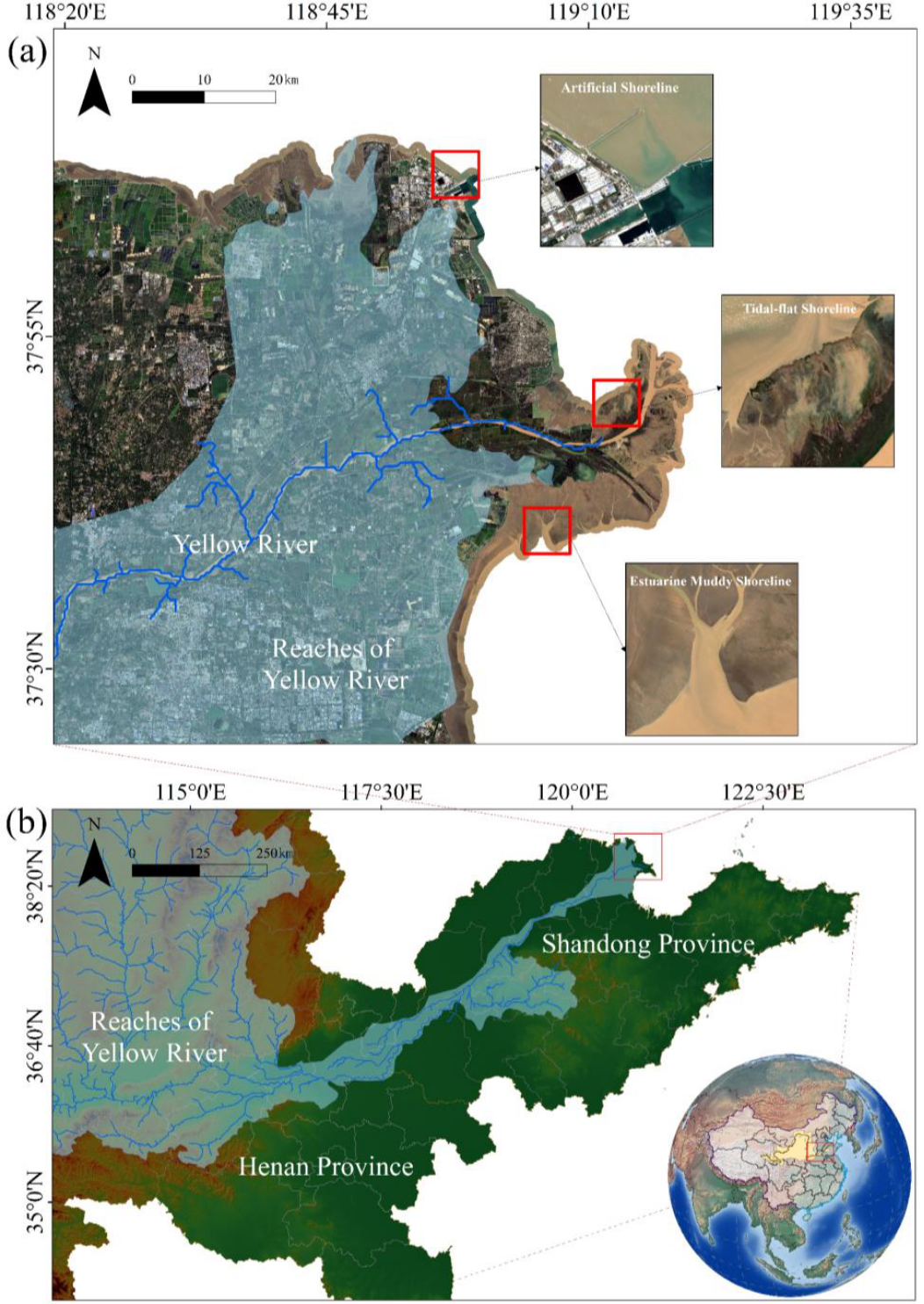
Figure 2.
Overall methodological framework of the study.
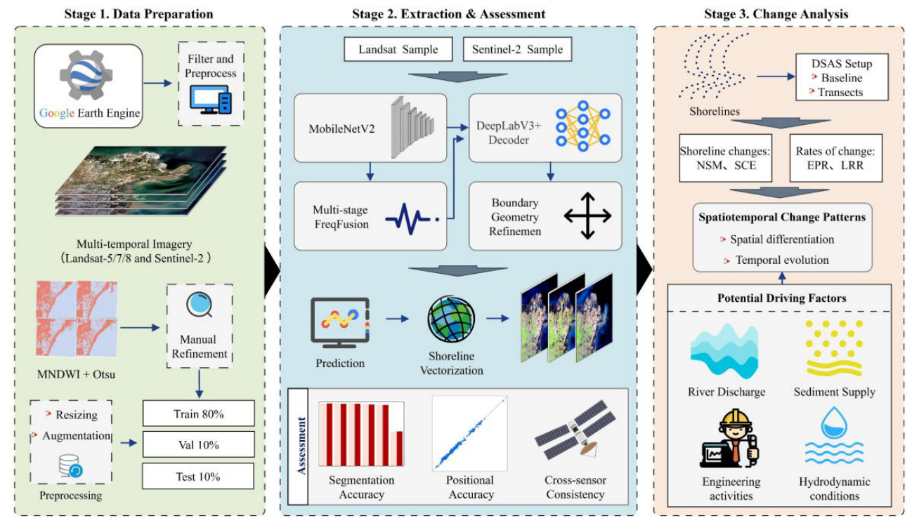
Figure 3.
Architecture of the MFGR-DeepLabV3+ model.
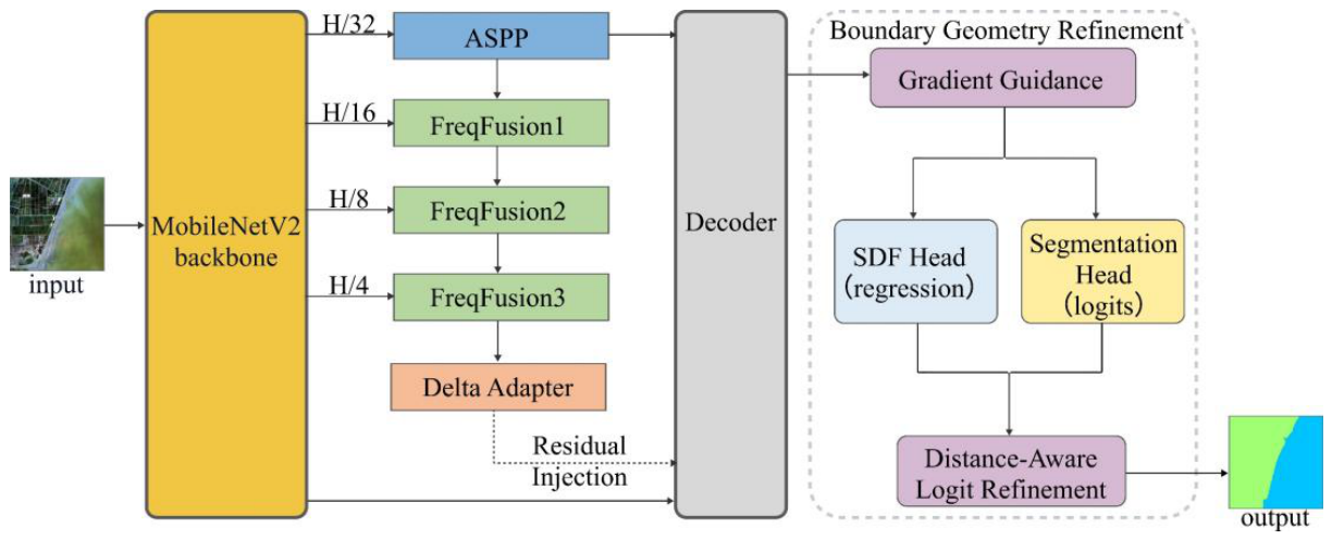
Figure 4.
Positional accuracy of model-derived shorelines evaluated using imagery from different sensors: (a) Distributions of signed horizontal errors for different sensors across shoreline sectors. (b) Pointwise shoreline offsets along transects for Landsat-5. (c) Pointwise shoreline offsets along transects for Landsat-7. (d) Pointwise shoreline offsets along transects for Landsat-8. (e) Pointwise shoreline offsets along transects for Sentinel-2. Positive and negative values indicate seaward and landward offsets relative to the manually interpreted reference shoreline, respectively.
Figure 4.
Positional accuracy of model-derived shorelines evaluated using imagery from different sensors: (a) Distributions of signed horizontal errors for different sensors across shoreline sectors. (b) Pointwise shoreline offsets along transects for Landsat-5. (c) Pointwise shoreline offsets along transects for Landsat-7. (d) Pointwise shoreline offsets along transects for Landsat-8. (e) Pointwise shoreline offsets along transects for Sentinel-2. Positive and negative values indicate seaward and landward offsets relative to the manually interpreted reference shoreline, respectively.
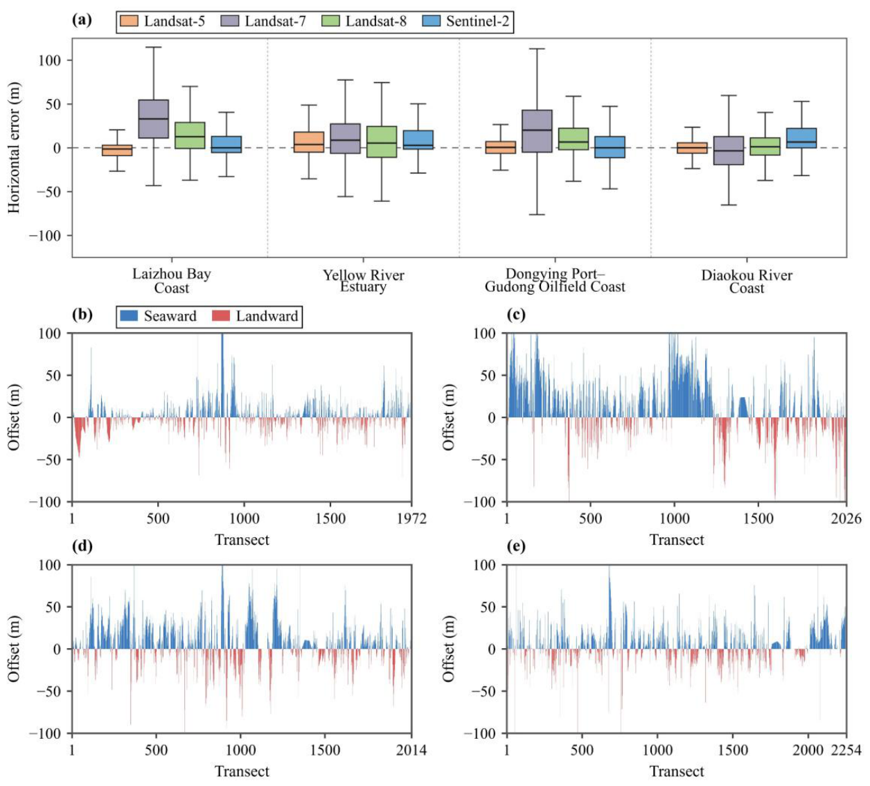
Figure 5.
Cross-sensor consistency between shoreline positions derived from Landsat-8 and Sentinel-2: (a–c) regression analyses of shoreline positions with the 1:1 reference line. (d–f) corresponding Bland–Altman difference analyses.
Figure 5.
Cross-sensor consistency between shoreline positions derived from Landsat-8 and Sentinel-2: (a–c) regression analyses of shoreline positions with the 1:1 reference line. (d–f) corresponding Bland–Altman difference analyses.
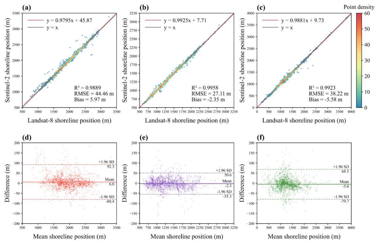
Figure 6.
Segmentation results produced by different models on the Landsat test set, with yellow denoting water, purple denoting segmented land, and red boxes highlighting regions of interest for comparison; the first and second columns show the remote sensing imagery and reference labels, respectively, the subsequent columns show predictions generated by the different models, and each row represents a different study location.
Figure 6.
Segmentation results produced by different models on the Landsat test set, with yellow denoting water, purple denoting segmented land, and red boxes highlighting regions of interest for comparison; the first and second columns show the remote sensing imagery and reference labels, respectively, the subsequent columns show predictions generated by the different models, and each row represents a different study location.
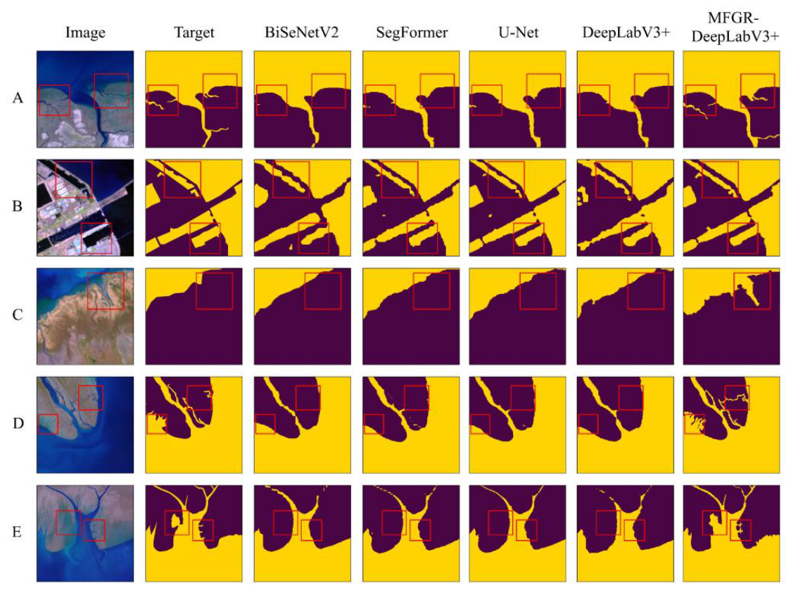
Figure 7.
Segmentation results produced by different models on the Sentinel-2 test set, with yellow denoting water, purple denoting segmented land, and red boxes highlighting regions of interest for comparison; the first and second columns show the remote sensing imagery and reference labels, respectively, the subsequent columns show predictions generated by the different models, and each row represents a different study location.
Figure 7.
Segmentation results produced by different models on the Sentinel-2 test set, with yellow denoting water, purple denoting segmented land, and red boxes highlighting regions of interest for comparison; the first and second columns show the remote sensing imagery and reference labels, respectively, the subsequent columns show predictions generated by the different models, and each row represents a different study location.
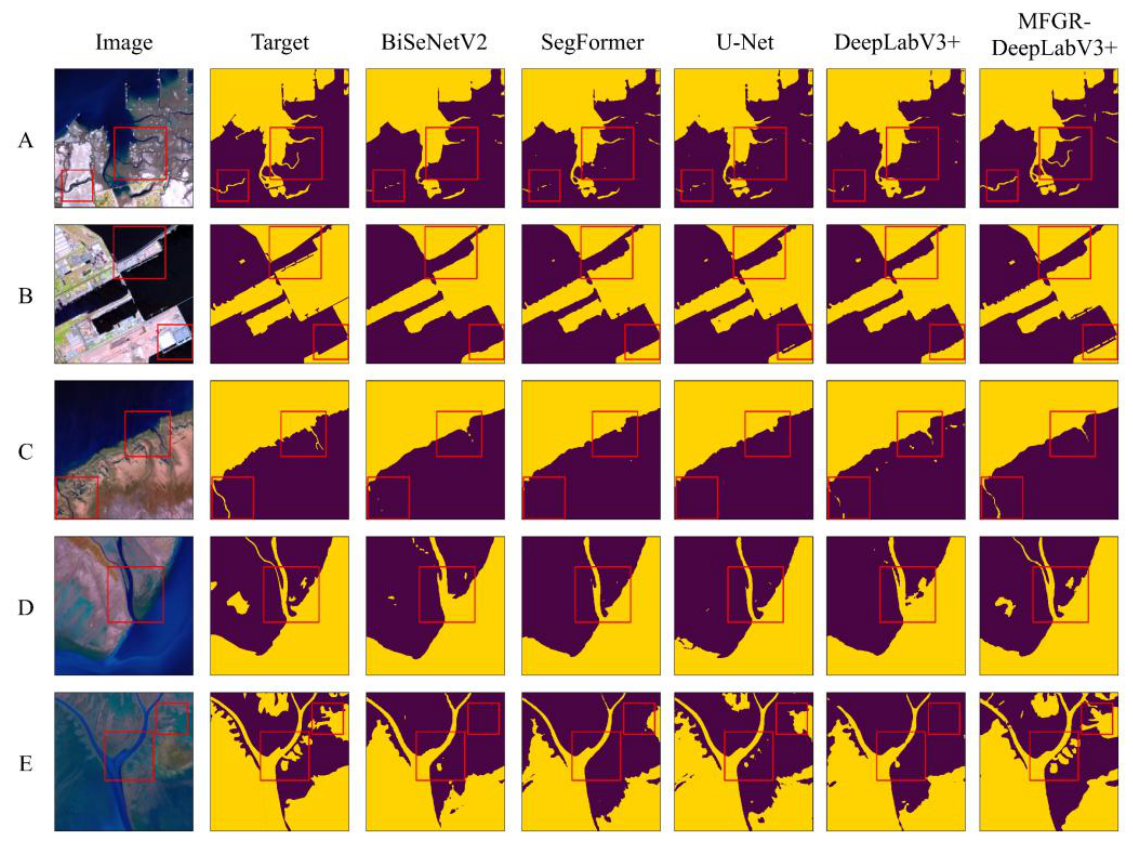
Figure 8.
Shoreline change at the Yellow River mouth: (a) Time-series heatmap showing relative changes in shoreline position since 1990. (b-d) Shoreline trend metrics (LRR and EPR) for 1990–2025, 1990–2005 and 2005–2025.
Figure 8.
Shoreline change at the Yellow River mouth: (a) Time-series heatmap showing relative changes in shoreline position since 1990. (b-d) Shoreline trend metrics (LRR and EPR) for 1990–2025, 1990–2005 and 2005–2025.
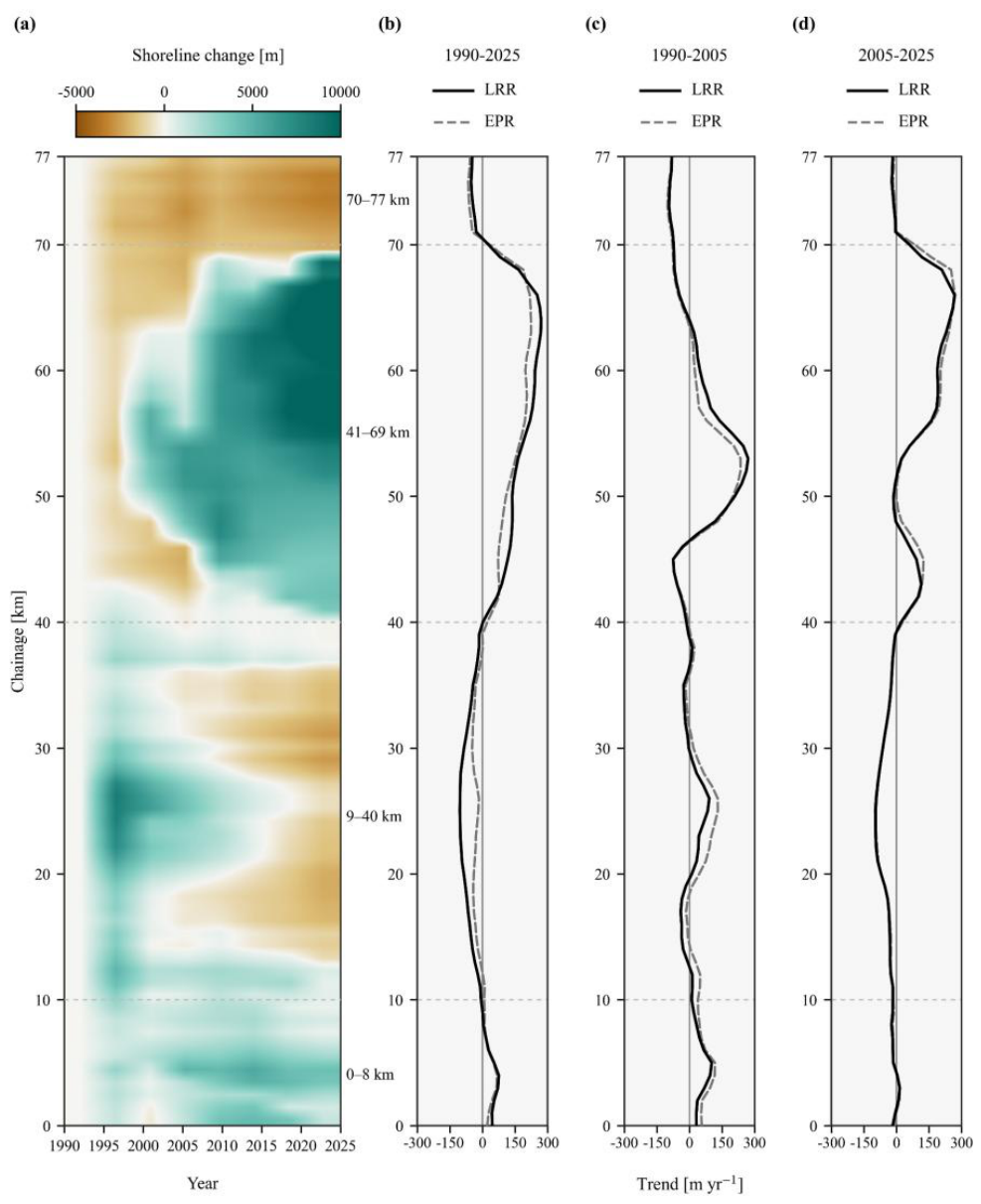
Figure 9.
Spatial patterns of shoreline change along the Laizhou Bay sector: (a) Distribution of Net Shoreline Movement (NSM). (b) Distribution of Shoreline Change Envelope (SCE). (c) Distribution of Linear Regression Rate (LRR). (d) Alongshore variations in SCE and NSM (upper panel) and LRR (lower panel).
Figure 9.
Spatial patterns of shoreline change along the Laizhou Bay sector: (a) Distribution of Net Shoreline Movement (NSM). (b) Distribution of Shoreline Change Envelope (SCE). (c) Distribution of Linear Regression Rate (LRR). (d) Alongshore variations in SCE and NSM (upper panel) and LRR (lower panel).
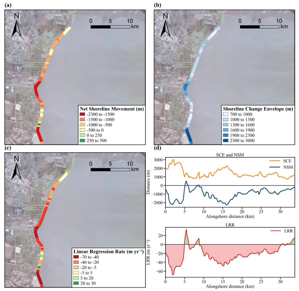
Figure 10.
Spatial patterns of shoreline change along the Diaokou River mouth sector: (a) Distribution of Net Shoreline Movement (NSM). (b) Distribution of Shoreline Change Envelope (SCE). (c) Distribution of Linear Regression Rate (LRR). (d) Alongshore variations in SCE and NSM (upper panel) and LRR (lower panel), with the vertical dashed line indicating the boundary between the two alongshore transect sequences.
Figure 10.
Spatial patterns of shoreline change along the Diaokou River mouth sector: (a) Distribution of Net Shoreline Movement (NSM). (b) Distribution of Shoreline Change Envelope (SCE). (c) Distribution of Linear Regression Rate (LRR). (d) Alongshore variations in SCE and NSM (upper panel) and LRR (lower panel), with the vertical dashed line indicating the boundary between the two alongshore transect sequences.
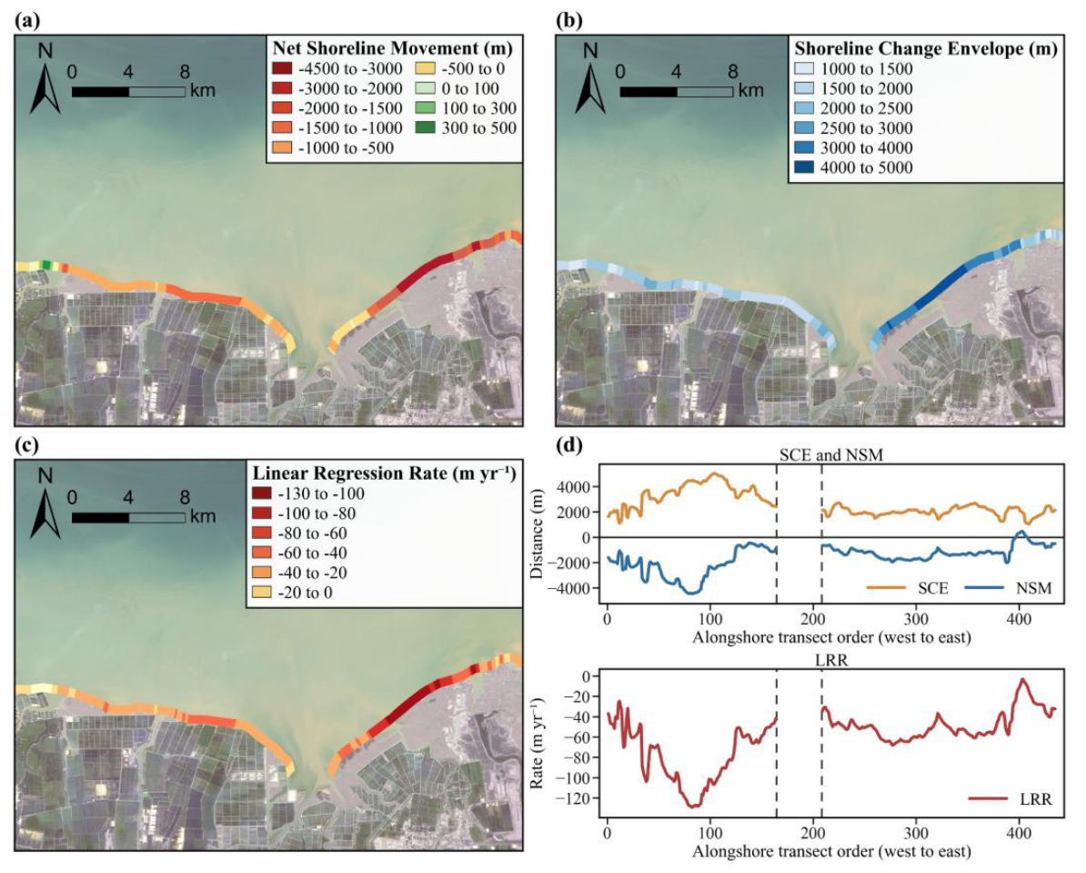

Table 1.
Acquisition details of satellite imagery for selected years used in shoreline analysis.
| Date | Satellite | Level | Sensor | Pixel Spacing (m) |
|---|---|---|---|---|
| 1990-06-16 | Landsat-5 | L2SP | TM | 30 |
| 1995-05-29 | Landsat-5 | L2SP | TM | 30 |
| 2000-05-02 | Landsat-7 | L2SP | ETM+ | 30 |
| 2005-05-08 | Landsat-5 | L2SP | TM | 30 |
| 2010-06-07 | Landsat-5 | L2SP | TM | 30 |
| 2015-05-04 | Landsat-8 | L2SP | OLI | 30 |
| 2020-05-01 | Sentinel-2 | Level-2A | MSI | 10 |
| 2025-06-04 | Sentinel-2 | Level-2A | MSI | 10 |
Table 2.
Ablation results on the Sentinel-2 test set.
| Model | Multi-stage FreqFusion | Boundary Geometry Refinement | mIoU | F1 Score | BIoU | ASSD | HD95 |
|---|---|---|---|---|---|---|---|
| Baseline | - | - | 0.8901 | 0.9419 | 0.4066 | 13.4754 | 50.9311 |
| Baseline + Multi-stage FreqFusion |
√ | - | 0.9066 | 0.9455 | 0.4305 | 12.6498 | 46.5788 |
| Baseline + Boundary Geometry Refinement |
- | √ | 0.8986 | 0.9440 | 0.4435 | 12.3076 | 45.8987 |
| MFGR-DeepLabV3+ (ours) | √ | √ | 0.9107 | 0.9482 | 0.4510 | 10.9239 | 43.7556 |
Table 3.
Ablation results on the Landsat test set.
| Model | Multi-stage FreqFusion | Boundary Geometry Refinement | mIoU | F1 Score | BIoU | ASSD | HD95 |
|---|---|---|---|---|---|---|---|
| Baseline | - | - | 0.9091 | 0.9519 | 0.5146 | 8.5327 | 14.8573 |
| Baseline + Multi-stage FreqFusion |
√ | - | 0.9167 | 0.9575 | 0.5202 | 7.6157 | 11.3643 |
| Baseline + Boundary Geometry Refinement |
- | √ | 0.9126 | 0.9560 | 0.5335 | 5.1038 | 9.8768 |
| MFGR-DeepLabV3+ (ours) | √ | √ | 0.9224 | 0.9592 | 0.5554 | 4.8462 | 6.6754 |
Table 4.
Summary statistics of DSAS metrics for different shoreline sectors of the Yellow River Delta.
Table 4.
Summary statistics of DSAS metrics for different shoreline sectors of the Yellow River Delta.
| Metric | Statistic | Laizhou Bay Coast | Yellow River Estuary | Dongying Port–Gudong Oilfield Coast | Diaokou River Coast | Total |
|---|---|---|---|---|---|---|
| SCE | Average distance (m) | 1513.09 | 6033.27 | 3333.98 | 2806.68 | 3568.84 |
| Minimum distance (m) | 811.63 | 104.29 | 9.4 | 807.77 | 9.4 | |
| Maximum distance (m) | 3005.86 | 14126.04 | 14293.68 | 6674.29 | 14293.68 | |
| NSM | Average distance (m) | -1071.72 | 1568.01 | 1323.48 | -2111.31 | 290.05 |
| Erosional transects (%) | 96.39 | 44.37 | 37.50 | 97.32 | 60.09 | |
| Maximum negative distance (m) | -2244.31 | -5444.55 | -2983.11 | -6248.99 | -6248.99 | |
| Accretional transects (%) | 3.61 | 55.63 | 39.29 | 2.68 | 29.97 | |
| Maximum positive distance (m) | 414.52 | 12521.73 | 13229.60 | 413.84 | 13229.60 | |
| EPR | Average rate (m/yr) | -30.65 | 44.84 | 37.85 | -60.38 | 8.30 |
| Maximum erosion rate (m/yr) | -64.18 | -155.70 | -85.31 | -178.71 | -178.71 | |
| Maximum accretion rate (m/yr) | 11.85 | 358.10 | 378.34 | 11.84 | 378.34 | |
| LRR | Average rate (m/yr) | -24.31 | 43.66 | 34.85 | -69.09 | 5.57 |
| Erosional transects (%) | 89.16 | 46.48 | 38.57 | 100.00 | 60.70 | |
| Maximum erosion rate (m/yr) | -67.78 | -199.91 | -201.11 | -182.19 | -201.11 | |
| Accretional transects (%) | 10.84 | 53.52 | 33.57 | 0.00 | 27.37 | |
| Maximum accretion rate (m/yr) | 26.41 | 413.27 | 420.92 | - | 420.92 |
Disclaimer/Publisher’s Note: The statements, opinions and data contained in all publications are solely those of the individual author(s) and contributor(s) and not of MDPI and/or the editor(s). MDPI and/or the editor(s) disclaim responsibility for any injury to people or property resulting from any ideas, methods, instructions or products referred to in the content. |
© 2026 by the authors. Licensee MDPI, Basel, Switzerland. This article is an open access article distributed under the terms and conditions of the Creative Commons Attribution (CC BY) license (http://creativecommons.org/licenses/by/4.0/).
Copyright: This open access article is published under a Creative Commons CC BY 4.0 license, which permit the free download, distribution, and reuse, provided that the author and preprint are cited in any reuse.