
Submitted:
22 September 2026
Posted:
23 September 2026
You are already at the latest version
Abstract
Remote sensing captions often combine domain terms, object relations, and scene context, while the corresponding images contain targets that occupy markedly different spatial scales. A single global text vector and fixed-scale visual aggregation can therefore discard information needed for image-text alignment. We develop a CLIP-style dual encoder with three additions: a text encoder that fuses word-level, phrase-level, and sentence-level representations; a visual encoder that associates four feature levels and uses SAM-guided local views during training and validation; and a semantic membership-aware contrastive loss with detached, bounded weights for semantically close negatives. On cleaned RSICD, the model obtains 87.5% mAP and 78.3% Top-1 accuracy for in-domain prompt-based scene recognition. Under scene-constrained retrieval with transductive dual-softmax reranking, it reaches 34.37% mean recall, compared with 30.58% for RemoteCLIP and 30.39% for fully fine-tuned CLIP. Removing the text encoder, scale-aware visual branch, or membership-aware loss lowers mAP by 6.8, 6.3, and 7.8 percentage points, respectively. The deployable dual encoder has approximately 59.7 million trainable parameters. These results apply to daytime optical imagery, a cleaned closed-category benchmark, in-domain prompts, and a fixed-gallery retrieval protocol.
Keywords:
remote sensing
; CLIP adaptation
; image-text retrieval
; multi-scale representation
; scene recognition
1. Introduction
Text-based access to Earth observation archives depends on connecting image content with captions, geographic annotations, and domain knowledge[1]. This connection supports semantic search and scene-level interpretation across heterogeneous remote sensing products[2], but it is difficult to learn when sensors, spatial resolutions, and description styles vary.
Vision-language models provide a shared representation for image retrieval, scene interpretation, and geospatial knowledge discovery. CLIP[3] is an attractive starting point because its contrastive objective supports transfer through natural-language supervision. Its pre-training data and architecture, however, were developed for natural images and generic captions rather than nadir-view Earth observation scenes[4].
Three transfer failures are especially relevant here. First, remote sensing captions place object names, attributes, spatial relations, and scene context in the same sentence, so an end-of-text embedding can obscure local terminology. Second, a scene may contain both a large land-cover structure and small but diagnostic objects, which are easily diluted by global visual pooling. Third, unmatched pairs are not equally unrelated: airports and industrial areas, for example, can share paved surfaces and geometric patterns. The study addresses these semantic-granularity, visual-scale, and negative-pair ambiguities.
Work on scale-adaptive patching and boundary-preserving segmentation shows why local spatial evidence matters in high-resolution remote sensing[5,6]. We use this observation without turning retrieval into a segmentation task. SAM supplies candidate crops for local-view augmentation, whereas the downstream model remains a dual encoder. The complete framework combines multi-granularity text encoding, hierarchical scale-aware visual features, SAM-guided training views, and a membership-aware contrastive objective. Experiments are limited to daytime optical imagery from RSICD and a restricted scene adaptation dataset; no large-scale remote sensing re-pretraining is used.
The study makes four technical contributions:
(1) We introduce a multi-granularity text encoder retains word-level, phrase-level, and sentence-level information and combines the three branches by cross-granularity attention.
(2) We introduce a scale-aware visual encoder links four receptive-field configurations to hierarchical feature maps, refines each level independently, and combines level descriptors through self-attention and gated concatenation.
(3) SAM-guided local-view augmentation adds object-focused evidence during training and validation without detector labels; inference uses only the dual encoder.
(4) A semantic membership-aware objective modifies InfoNCE[7] with detached weights and a bounded discount, reducing the penalty for semantically close negatives while keeping every negative contribution positive.
2. Related Work
2.1. Vision-Language Pre-Training and CLIP-Based Multimodal Learning
Vision-language pre-training differs mainly in where cross-modal interaction occurs. ViLBERT[8] maintains separate visual and linguistic streams linked by co-attention, whereas UNITER[9] uses joint multimodal encoding with region-level visual inputs. Both established explicit region-token interaction, but their detector-dependent pipelines are less direct than a retrieval-oriented dual encoder.
Later models reduced the cost of visual processing or changed the order of alignment and fusion. ViLT[10] projects image patches directly into a Transformer; ALBEF[11] aligns unimodal features before multimodal fusion; BLIP[12] combines understanding and generation objectives; and FLIP[13] masks image patches during pre-training. These designs improve general vision-language learning, yet they do not explicitly model the semantic hierarchy and scale distribution of remote sensing scenes.
CLIP learns separate image and text embeddings and compares them in a shared space. This structure is efficient for retrieval, but its text output is a single sentence vector and its visual encoder is tuned to natural-image statistics. Direct transfer can therefore miss local domain terms and small scene elements that determine remote sensing categories.
Remote sensing adaptations address this domain gap through parameter-efficient transfer[14], visual priors[15], or domain-specific pre-training[16]. RemoteCLIP[17] and GeoRSCLIP[18] show the value of large remote sensing image-text corpora. The present study asks a narrower question: whether explicit semantic granularity, visual scale, and graded negative-pair weighting can improve a CLIP-style model when large-scale domain re-pretraining is unavailable.
2.2. Fine-Grained Semantic Modeling for Multimodal Alignment
A remote sensing caption may specify a target, its attributes, its relation to nearby objects, and the wider geographic setting. Compressing these elements directly into one global embedding can weaken the distinctions between scenes that share most of their content. Fine-grained alignment therefore requires local lexical and relational features to remain available when the sentence representation is formed.
Hierarchical text encoding and multi-level alignment provide relevant precedents. Text-focused alignment has been studied in vision-language models[19], while multi-level methods align local and global representations at different stages[20,21]. These studies motivate structured text features, but they do not determine how remote sensing terminology should be combined with phrase and sentence context.
Our design uses WordPiece tokenization to retain subword cues in abbreviations and compound identifiers, then processes the resulting sequence through word-level, phrase-level, and sentence-level branches. It does not add a character encoder. Cross-granularity attention combines the branches before projection to the shared embedding space.
2.3. Multi-Scale Visual Representation and Semantic-Aware Contrastive Learning
Spatial scale changes the evidence available to a retrieval model. Vehicles and individual buildings occupy small regions, whereas airports, ports, and urban blocks require broader context. Feature pyramids address related variation in object detection, but image-text retrieval must convert the resulting local and global evidence into one embedding rather than predict boxes or masks.
Feature-fusion architectures[22,23] and domain-adaptation methods[24,25] provide mechanisms for combining levels or transferring visual representations. Remote sensing vision-language models also use prior knowledge, calibration, and specialized pre-training. What remains unresolved for the present setting is how to preserve level-specific information while producing a compact dual-encoder representation.
The contrastive objective introduces a second problem. InfoNCE[7] treats all unmatched pairs as negatives, although their gradients already vary with similarity. In remote sensing, semantically related categories can share spectral responses, textures, or layouts. Uniformly enforcing category separation can therefore conflict with partial scene overlap.
Soft objectives and adaptive weighting have been investigated as alternatives[26,27]. The method proposed here uses a more restricted intervention: a similarity-derived membership weight can only reduce a negative term within a fixed bound, and the weight is detached so it cannot directly attract an unmatched pair.
Table 1 summarizes the resulting distinction. The framework changes both encoders rather than adding an adapter, uses SAM only to generate unlabeled local training views, preserves four visual levels through self-attention and gated concatenation, and applies bounded membership weights to negative terms. Because evaluation uses two modest optical datasets and no large-scale domain re-pretraining, the model is an application-specific adaptation rather than a remote sensing foundation model.
3. Methods
3.1. Task Formulation and Framework Overview
Global text aggregation, limited explicit scale modeling, and the absence of se-mantic weighting among negatives can constrain CLIP-style alignment on remote sensing imagery. We address these three gaps with three interacting modules to map a remote sensing image and its caption to a 512-dimensional shared space for bidirectional retrieval and prompt-based scene recognition. Figure 1 shows the three interacting module: a multi-granularity text encoder, a scale-aware visual encoder, and a semantic membership-aware contrastive objective. SAM-guided crops enter the visual branch during training and validation but are not required at inference.
The text encoder keeps lexical, phrase, and sentence information separate until attention fusion. The visual encoder associates four spatial resolutions with hierarchical ResNet features and combines the resulting level descriptors. The loss then uses semantic membership to distinguish semantically close negatives from unrelated negatives while retaining the bidirectional contrastive formulation.
Given paired samples , the image and text encoders produce representations and . Both are projected to 512 dimensions, matching the CLIP embedding width. Training increases the similarity of matched pairs and preserves separation from unmatched pairs, with the negative penalty adjusted as described in Section 3.5.
The complete feature extraction and alignment process can be formulated as:
Here, and denote the scale-aware visual encoder and multi-granularity text encoder; and are their outputs.
3.2. Multi-granularity Semantic Modeling
CLIP forms its text embedding from the end-of-text token after Transformer encoding. Although token interactions are contextualized, the output does not expose separate lexical, phrasal, and sentence representations. We retain these three granularities explicitly. WordPiece tokenization supplies subword cues for abbreviations and compound identifiers, so no character-level branch is introduced.
Figure 2 groups the text pathway into semantic hierarchy decomposition, parallel branch encoding, and cross-granularity attention fusion.
3.2.1. Semantic Hierarchy Decomposition
Remote sensing captions often encode several semantic roles at once. In “a long bridge crossing a river near dense residential buildings,” the nouns identify objects, the modifiers describe geometry and density, and the prepositions specify spatial relations. The encoder therefore retains local units before combining them with sentence context.
From the perspective of semantic hierarchy decomposition, remote sensing text can be represented as a hierarchical structure:
where , , and denote word-level, phrase-level, and sentence-level semantic components, respectively.
WordPiece subwords enter all three branches. The word branch emphasizes object and attribute tokens; the phrase branch captures short-range combinations and spatial relations; and the sentence branch models the full caption. These roles define the semantic hierarchy used below.
Before projection to the shared space, the model maintains local detail and global context in a structured representation:
The conditional form indicates that local components are interpreted in the context of the complete sentence rather than used as independent descriptors.
3.2.2. Multi-Branch Encoder Architecture
The three branches process the same tokenized caption but use different receptive fields. This parallel design exposes information that would otherwise be available only implicitly inside a single sentence-level Transformer output.
The sentence branch uses a Transformer with positional and token-type embeddings. Sequences are limited to 77 tokens, and the hidden state is linearly projected to 512 dimensions to obtain .
The word branch applies a convolution with kernel size and the stated channel configuration, followed by a Transformer layer with hidden dimension 256. Its output is .
The phrase branch uses a convolution with kernel size and 128 channels, followed by Transformer refinement, to produce .
[WORD], [PHRASE], and [SENTENCE] token-type embeddings identify the branch roles. Each output is normalized and projected to 512 dimensions before fusion.
3.2.3. Cross-Granularity Attention Fusion
The branches should not contribute equally to every caption. Concatenation would retain all components but would not condition their importance on sentence content. We instead use the sentence representation as a global query over the word and phrase features.
The sentence-level representation provides the query, and the word-level and phrase-level representations provide local semantic evidence. Their first attention operation is:
Here, denotes multi-head attention. The attention weights select local components in the context of the complete description.
A residual connection and feature normalization yield the final fused representation:
Here, is the feature projection and is layer normalization. The fused text vector remains 512-dimensional.
This fusion retains lexical and relational cues while keeping them conditioned on sentence meaning.
3.3. Scale-Aware Visual Encoding
Remote sensing scenes distribute evidence across markedly different spatial extents. A port requires broad layout information, whereas ships, vehicles, and individual buildings may occupy only a few local regions. The visual branch therefore uses hierarchical features rather than a single pooled map.
Global aggregation can suppress small but diagnostic targets, while fine features alone cannot represent the organization of large geographic structures. The proposed branch assigns fine and coarse receptive-field configurations to corresponding ResNet feature levels.
The branch produces one image embedding for alignment; it does not predict classes, boxes, or masks. It combines SAM-guided local-view augmentation with four-level feature extraction and hierarchical association.
Figure 3 shows the two inputs and the subsequent scale-aware feature pathway.
3.3.1. SAM-Guided Local-View Augmentation
A whole-scene CLIP representation may overlook a target that occupies a small image fraction. Local-view augmentation supplies an additional crop when SAM identifies a usable region. SAM is run offline before image encoding. It generates candidate regions without target labels or detector supervision. The crop is an auxiliary visual input, not a segmentation output. Region selection uses the implementation's visual-similarity and spatial-consistency criteria.
For image , a selected SAM proposal is cropped to form . If no proposal passes the reliability criterion, the original image is reused, which keeps the input pathway defined for every sample.
The global image and local view are encoded independently:
Here, is the CLIP visual encoder, and and are the global and local representations.
The coefficient controls their relative contributions. This operation adds local evidence without introducing a detector at inference. The deployment-time network remains the dual encoder.
3.3.2. Scale-Aware Feature Representation
The scale-aware prior configuration allocates receptive fields to visual patterns of different extent. Although expressed with scale and aspect-ratio priors, it is used to organize representation learning rather than to produce detections.
The original three scales , , and are extended to four levels: , , , and . The added fine scale targets small structures, and the coarse scales retain wider scene context.
The scale set is:
Here, is the receptive-field scale set. The fine scales and correspond to the 56 × 56 and 28 × 28 feature maps (P2 and P3), which retain local boundaries and small objects. The coarse scales and correspond to the 14 × 14 and 7 × 7 maps (P4 and P5), which encode larger structures and scene context.
The aspect-ratio set is expanded to cover compact and elongated structures:
Here, lists the candidate shapes used by the encoder.
Together, the four scales and expanded aspect ratios provide complementary local and contextual features.
3.3.3. Hierarchical Feature Association
Feature depth is matched to spatial scale. Shallow, high-resolution maps retain edges and textures, whereas deeper maps contain stronger semantic abstraction. Fine-scale configurations are associated with shallow feature levels, and coarse configurations with deeper levels. This pairing avoids forcing all spatial evidence through a single resolution.
For a ResNet-based extractor[28,29,30], the intermediate maps are:
where , , , and denote the four network stages.
Their aggregation is formulated as:
where denotes hierarchical fusion of the level-specific features.
Channel attention then recalibrates the aggregated responses:
where and are learnable transformations, is the nonlinear activation, is the sigmoid function, and denotes element-wise multiplication.
The visual vector is finally projected to the 512-dimensional text space:
where is the projection layer.
The aggregation differs from a standard FPN in three implementation choices. Each pyramid level has an independent residual head with two 3 × 3 convolutions, normalization, and nonlinear activation. The four globally pooled descriptors are then treated as a sequence and processed by multi-head self-attention. Finally, softmax-normalized gates modulate the concatenated descriptors rather than summing them, preserving level-specific information in the final image embedding.
3.4. Cross-modal Feature Alignment
3.4.1. Feature Normalization in the Shared Space
Image and text features are linearly projected and normalized before comparison. This removes feature-magnitude differences between modalities and makes cosine similarity depend on embedding direction.
The projected visual feature and text feature are normalized as follows:
where and are the normalized image and text embeddings.
Both embeddings have 512 dimensions, so they can be compared directly.
3.4.2. Cross-Modal Similarity
Cosine similarity measures the correspondence between an image and a caption:
where is the similarity between image and text .
Pairwise similarities for a batch form the matrix used by the contrastive objective.
A temperature coefficient scales the logits:
Smaller produces a sharper distribution; larger values smooth it.
3.4.3. Cross-Modal Feature Interaction
Before contrastive optimization, the model combines the multi-granularity text vector and scale-aware image vector to emphasize dimensions supported by both modalities.
This interaction is learned jointly with the encoders and does not require an additional hand-crafted correction at inference.
The fused representation is:
where and are balancing coefficients and denotes element-wise multiplication. The interaction term increases the contribution of dimensions with aligned image and text responses.
3.5. Semantic Membership-Aware Contrastive Learning
Unmatched remote sensing pairs can still share scene content. Airports and industrial areas contain similar paved regions, and bridges and ships can have elongated shapes. The objective therefore discounts, but does not remove, the penalty assigned to high-membership negatives.
3.5.1. Semantic Membership Estimation
For image and text , the membership weight lies in [0, 1]; larger values indicate greater semantic proximity.
A row-adaptive sigmoid converts similarity to membership:
Here, is the logistic function, k is a learnable slope initialized to 5.0, and is the row mean. Because maps to (0, 1), the weights remain bounded. Diagonal values are set to , so matched pairs are not discounted.
A second threshold δ gates low-confidence associations before the weights enter the loss:
Here, is the indicator function. The row mean μ_i centers similarity within each row but remains dependent on batch composition. The scalar δ instead gates the raw cosine similarity: pairs below δ keep the full negative penalty, even if they exceed a weak row mean. Diagonal entries are excluded from discounting.
3.5.2. Membership-aware Contrastive Objective
The membership weight changes only the negative terms in the partition function. Standard InfoNCE already produces similarity-dependent gradients; the additional factor reduces the contribution of negatives estimated to be semantically close.
The image-to-text partition is:
The text-to-image loss is defined analogously:
With λ ∈ [0, 0.95], the factor (1 − λ·) remains in [0.05, 1]. Thus, the discount cannot invert or eliminate a negative penalty. Log-sum-exp is used for numerical stability.
The final loss averages the two retrieval directions:
Matched pairs retain the full alignment term. High-membership negatives receive a smaller penalty, whereas low-membership negatives retain the standard contribution.
Because membership is computed from the similarity matrix being optimized, gradients through the weights could create a feedback path. We therefore calculate with stop-gradient. The weight changes penalty magnitude but cannot directly encourage an unmatched pair to become more similar. Together with the positive lower bound and δ gate, an erroneous membership estimate can only attenuate a penalty.
This formulation performs bounded gradient reweighting rather than redefining unmatched pairs as positives.
4. Experiments and Results
4.1. Datasets and Evaluation Metrics
RSICD[31] is the primary benchmark and originally contains 10,921 images with 54,605 captions. We retain the official image-level split. Before training, captions duplicated across different images are removed; within-image near duplicates are removed at a Jaccard threshold of 0.9; captions without a geographic or spatial entity are filtered; and lightweight keyword annotations are appended online only to training captions.
After cleaning, RSICD contains 6,922 images and 12,964 captions. The train/validation/test splits contain 5,177/740/1,005 images and 8,692/1,539/2,733 captions, with 1.68/2.08/2.72 captions per image. Merging the three residential subclasses leaves 28 categories. This preprocessing changes the task relative to raw RSICD: it removes one source of ambiguous positives, but the score effect has not been isolated by a direct comparison. RSICD[31] is used for both prompt-based scene recognition and scene-constrained bidirectional retrieval.
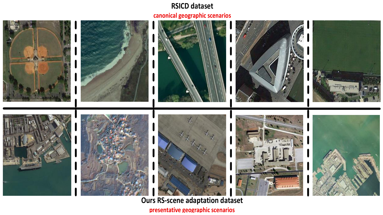
The second dataset contains 4,622 optical images of man-made target scenes and one bilingual caption per image. Its four functional groups are port and shipyard facilities, surface and industrial vessels, ground vehicles, and ground installation sites.
Captions follow a common template covering viewpoint, target category and count, surface or berthing context, and surrounding land cover. Splits are assigned by physical target or site so that near-duplicate views do not cross partitions. Usage restrictions prevent public release, which limits independent reproduction despite the documented annotation and grouping rules.
Figure 4.
Examples from RSICD and the remote sensing scene adaptation dataset.
4.1.1. Image-Text Retrieval Evaluation
Retrieval uses a scene-constrained RSICD protocol: queries and galleries belong to the 28 known scene categories. This closed taxonomy represents search within a predefined scene ontology, not open-world retrieval. Every baseline in Table 5 uses the same cleaned split, gallery, and ranking procedure.
Recall at K (R@K) records whether the matched item occurs among the top K results.
We report R@1, R@5, and R@10 for image-to-text (I2T) and text-to-image (T2I) retrieval. Mean recall (mR) is the average of all six values:
Throughout the paper, mR refers only to this bidirectional retrieval average. The mAP reported for scene recognition is a separate metric.
At test time, dual-softmax reranking recalibrates the cosine-similarity matrix using its row and column distributions:
where is the original similarity matrix and τ is the temperature.
The two directions are combined as:
where controls their relative contribution.
4.1.2. Prompt-Based Scene Recognition Evaluation
For prompt-based scene recognition, mean Average Precision (mAP) is adopted to evaluate whether the learned image-text representation can correctly identify semantic scene categories.
The average precision of each category is calculated according to the precision ranking of predicted semantic scores[34,35], and mAP averages over categories:
where is the number of scene categories.
This is an in-domain prompt evaluation because category labels affect prompt construction and training-time sampling. It is not cross-dataset zero-shot recognition. Table 2 shows that the five-template ensemble with normalized class names gives the highest validation setting, 87.5% mAP, and is used for the remaining recognition experiments.
4.2. Implementation and Comparison Protocol
Models are implemented in PyTorch (The version of PyTorch used was 1.8.0). The visual branch uses CLIP ResNet-50 because the scale-aware module requires the C2-C5 hierarchy, which a flat ViT-B/32 feature map does not provide. Training uses a batch size of 64 for 100 epochs. SAM crops are generated offline and excluded from training time; approximately 59.7 million trainable parameters belong to the deployable dual encoder. Dual-softmax reranking is applied only at test time and is not part of model training.
Recognition baselines are CLIP with ViT-B/32[3], ViLT[10], ALBEF[11], and BLIP[12]. Retrieval additionally compares SkyCLIP[36], CLIP-Adapter[37], RemoteCLIP[17], and fully fine-tuned CLIP[3]. Public pre-trained weights initialize all baselines, which are fine-tuned on the same data partitions and evaluated with the same task-specific protocols.
Optimization settings are kept fixed across the two datasets. This controls one source of variation but does not separate architecture, initialization, and data-composition effects.
4.3. Comparative Evaluation
The comparisons test prompt-based scene recognition on both datasets and scene-constrained bidirectional retrieval on RSICD. Results are interpreted within the shared training and evaluation settings defined above.
4.3.1. Comparison with State-of-the-Art Models
Table 3 reports prompt-based scene recognition on RSICD. The proposed model reaches 87.5% mAP and 78.3% Top-1 accuracy, compared with 74.8% and 65.2% for CLIP. It also exceeds ViLT, ALBEF, and BLIP under the same in-domain prompt protocol.
Relative to CLIP, the gains are 12.7 percentage points in mAP and 13.1 points in Top-1, with approximately 59.7 million rather than 151 million trainable parameters. Training takes 1.88 h versus 1.50 h, so parameter count does not translate directly into training time. The ablations in Section 4.4 separate the contributions of the three proposed components.
4.3.2. Results on the Scene Adaptation Dataset
To further evaluate the remote sensing semantic adaptation capability of the proposed framework, experiments are conducted on the remote sensing scene adaptation dataset. Table 4 reports in-domain prompt recognition on the restricted scene adaptation dataset. The proposed model obtains 88.2% mAP and 78.5% Top-1 accuracy, compared with 73.8% and 66.4% for CLIP. The mAP gain is larger than on RSICD, whereas the Top-1 gain is smaller; differences in category composition and supervision prevent attributing this contrast to one module.
The result is consistent with the intended use of domain-specific captions, which encode target relations, spatial arrangement, and functional attributes. Improvement on two separate in-domain evaluations shows that the architecture can use the available domain supervision. It does not establish cross-dataset generalization.
Category counts in the scene adaptation dataset range from 287 to 2,143 across four functional groups. Because aggregate retrieval recall would be dominated by this imbalance without category-wise analysis, retrieval is reported only on the more balanced RSICD scene-constrained protocol.
4.3.3. Scene-Constrained Image-Text Retrieval on RSICD
Table 5 reports I2T and T2I recall on the cleaned RSICD test set; mR averages the six recall values.

Table 5.
Scene-constrained image–text retrieval performance on RSICD.
| RSICD Dataset | |||||||
| Method | I2T | T2I | mR | ||||
| R@1 | R@5 | R@10 | R@1 | R@5 | R@10 | ||
| CLIP[3,38] | 6.77 | 15.37 | 23.15 | 5.01 | 15.75 | 24.21 | 15.04 |
| ALBEF[11,39] | 7.82 | 19.34 | 30.41 | 6.18 | 20.35 | 33.45 | 19.59 |
| BLIP[12,39] | 9.15 | 22.96 | 32.02 | 10.67 | 27.75 | 40.00 | 23.76 |
| SkyCLIP[36,40] | 6.59 | 16.10 | 26.53 | 7.14 | 22.34 | 34.29 | 18.83 |
| CLIP-Adapter[37,40] | 7.11 | 19.48 | 31.01 | 7.67 | 24.87 | 39.73 | 21.65 |
| RemoteCLIP[17,39] | 13.36 | 32.94 | 44.83 | 10.76 | 32.83 | 48.75 | 30.58 |
| Full-FT CLIP[3,40] | 13.54 | 30.83 | 43.46 | 11.55 | 33.14 | 49.83 | 30.39 |
| Ours | 17.36 | 35.84 | 50.85 | 15.64 | 34.51 | 51.99 | 34.37 |
The proposed model reaches 34.37% mR, 3.79 percentage points above RemoteCLIP and 3.98 points above fully fine-tuned CLIP. Its trainable parameter count is approximately 59.7 million, but efficiency relative to RemoteCLIP cannot be resolved without the exact evaluated backbone and trainable parameter count for that baseline.
The largest differences from CLIP occur at R@1: 17.36% versus 6.77% for I2T and 15.64% versus 5.01% for T2I. The comparison shows better first-rank retrieval in this setting, but it does not separate encoder effects from the proposed loss or establish superiority over adapter tuning beyond this protocol.
4.4. Ablation Studies
To investigate the contribution of each proposed component and understand the underlying mechanism of performance improvement, ablation experiments are conducted on the RSICD test set. Three key modules are individually removed or replaced, including the multi-granularity semantic modeling module, the scale-aware visual representation module, and the semantic membership-aware contrastive learning objective. Table 6 removes one component at a time on the RSICD prompt-recognition task.
Scheme A replaces the multi-granularity text encoder with the original single-level CLIP text representation. Scheme B removes the scale-aware priors and hierarchical feature association. Scheme C replaces the membership-aware objective with standard InfoNCE. Scheme D is the complete model.
Every single-component removal reduces both mAP and Top-1 accuracy. Without multi-granularity text encoding (Scheme A), mAP falls from 87.5% to 80.7% and Top-1 from 78.3% to 73.1%. The 6.8-point mAP loss is consistent with a contribution from explicit lexical and phrase features. The original CLIP text encoder mainly relies on global sentence-level embeddings, which may weaken fine-grained semantic concepts when descriptions contain multiple types of information. After removing this module, the model no longer has dedicated branches for lexical and phrase-level features; the lower recognition scores are consistent with a benefit from this explicit decomposition.
Removing the scale-aware visual branch (Scheme B) lowers mAP to 81.2% and Top-1 to 74.5%, decreases of 6.3 and 3.8 percentage points. This result supports using hierarchical visual evidence when local targets and global scene structure coexist. This result verifies that scale adaptation is an important factor for remote sensing visual representation learning. Remote sensing scenes usually contain objects with large variations in spatial coverage, and dominant background structures may suppress small but semantically meaningful objects during feature aggregation.
Replacing the proposed loss with InfoNCE (Scheme C) lowers mAP to 79.7% and Top-1 to 73.7%, decreases of 7.8 and 4.6 points. Among the three removals, this produces the largest mAP decrease in the tested configuration. This demonstrates that semantic-aware negative sample optimization is particularly beneficial for fine-grained discrimination in prompt-based scene recognition. In remote sensing scenarios, many categories exhibit similar spectral responses and spatial configurations, generating large numbers of hard negative samples. Conventional InfoNCE does not explicitly discount these samples according to semantic membership, which may introduce excessive optimization constraints. The proposed membership-aware objective modifies the contribution of negative samples according to semantic proximity, reducing unnecessary separation between semantically related categories while maintaining discrimination against irrelevant samples.
Table 7 tests how membership weights are computed. The detached default reaches 87.5% mAP and 78.3% Top-1; allowing gradients through the weights gives 72.9% and 69.8%, while fixed scene-label weights give 85.7% and 77.6%. This comparison supports detaching the weights in the tested configuration. The lower scores without detachment are consistent with the feedback concern discussed in Section 3.5.
5. Discussion
SAM generated a valid local proposal for 98.5% of training images and 97.4% of validation images, but coverage fell to 86.6% for meadow, 87.5% for forest, and 90.6% for desert. Texture-dominated scenes provide fewer discrete boundaries, so these samples more often use the global-view fallback. Removing SAM while retaining the other scale-aware operations lowers mAP from 87.5% to 83.3% and Top-1 from 78.3% to 77.4% (Table 8). Removing the entire scale-aware branch produces 81.2% mAP and 74.5% Top-1. SAM therefore contributes to the branch, especially to ranked category performance, but the current results do not identify which confusions it resolves. Because SAM is used during training and validation but not inference, the model also contains a train-test view mismatch; distilling local-view information into the global encoder is a direct way to test whether that gap can be reduced.
The retrieval and recognition protocols expose a second limitation. Dual-softmax reranking uses the full test-gallery score distribution, so Table 5 is not directly comparable with open-set retrieval or direct cosine ranking. Internal comparisons remain fair because every baseline uses the same gallery and reranking. Prompt formulation has an equally large effect: mAP ranges from 56.9% for attribute-enhanced prompts with raw class names to 87.5% for the five-template ensemble with normalized names. Bare class names also outperform the generic template “a photo of [class].” A plausible explanation is that the randomly initialized text encoder is trained on domain-specific captions, but the experiment does not isolate this mechanism. Prompt selection should therefore be performed on validation data for the intended domain.
The evidence is further bounded by model and data choices. The text encoder is trained from random initialization, and the visual backbone is a CLIP-initialized ResNet-50. Comparisons with language-pretrained text encoders, larger backbones, or hierarchical transformers remain open. All images are daytime RGB observations; photometric augmentation does not establish transfer to SAR, hyperspectral, or real night-time imagery.
Our future work should target the unresolved boundaries rather than add modules without diagnosis. Cross-dataset and cross-sensor tests with held-out categories would measure out-of-distribution behavior. A lightweight trainable proposal head could test whether local views can be learned end to end with lower preprocessing cost, and a high-resolution pathway could quantify the accuracy-cost trade-off at the finest feature level.
6. Conclusions
This study adapted a CLIP-style dual encoder to remote sensing by combining multi-granularity text encoding, hierarchical scale-aware visual features with SAM-guided training views, and a detached semantic membership-aware contrastive loss. On cleaned RSICD, the model achieves 87.5% mAP for in-domain prompt-based scene recognition and 34.37% mR for scene-constrained retrieval with transductive dual-softmax reranking, using approximately 59.7 million trainable parameters. These values apply to the reported daytime optical datasets, prompt construction, cleaned category taxonomy, and fixed-gallery protocol. The present experiments do not establish open-set, cross-dataset, or cross-sensor generalization, and SAM is unavailable at inference. Future evaluation should address these boundaries and test whether local-view knowledge can be transferred to the deployment-time encoder.
Author Contributions
Conceptualization, L.X. and Q.Z.; methodology, L.X. and Q.Z.; validation, L.X. and T.L.; formal analysis, Q.Z. and L.W.; investigation, Q.Z. and Y.L.; resources, Y.L. and T.L.; data curation, Y.L.; writing—original draft preparation, L.X. and L.W.; writing—review and editing, Q.Z. and T.L.; supervision, Q.Z. All authors have read and agreed to the published version of the manuscript.
Funding
This research received no external funding.
Data Availability Statement
The RSICD dataset is publicly available. The scene adaptation dataset constructed in this study is subject to usage restrictions and cannot be publicly released; its annotation procedure and partitioning principles are described in Section 4.1. Further inquiries can be directed to the authors.
Conflicts of Interest
The authors declare no conflicts of interest.
References
- Li, J.; Hong, D.; Gao, L.; Yao, J.; Zheng, K.; Zhang, B.; Chanussot, J. Deep Learning in Multimodal Remote Sensing Data Fusion: A Comprehensive Review. Int. J. Appl. Earth Obs. Geoinf. 2022, 112, 102926. [Google Scholar] [CrossRef]
- Li, S.; Tang, H. Multimodal Alignment and Fusion: A Survey 2025. arXiv 2025, arXiv:2411.170402018. [Google Scholar]
- Radford, A.; Kim, J.W.; Hallacy, C.; Ramesh, A.; Goh, G.; Agarwal, S.; Sastry, G.; Askell, A.; Mishkin, P.; Clark, J.; et al. Learning Transferable Visual Models From Natural Language Supervision. arXiv 2021, arXiv:2103.00020. [Google Scholar] [CrossRef]
- Jia, C.; Yang, Y.; Xia, Y.; Chen, Y.-T.; Parekh, Z.; Pham, H.; Le, Q.V.; Sung, Y.; Li, Z.; Duerig, T. Scaling Up Visual and Vision-Language Representation Learning With Noisy Text Supervision. arXiv 2102.05918. 2021. [Google Scholar] [CrossRef]
- Liu, Y.; Shi, S.; Wang, J.; Zhong, Y. Seeing Beyond the Patch: Scale-Adaptive Semantic Segmentation of High-Resolution Remote Sensing Imagery Based on Reinforcement Learning. In Proceedings of the 2023 IEEE/CVF International Conference on Computer Vision (ICCV), Paris, France, October 1 2023; IEEE; pp. 16822–16832. [Google Scholar]
- Sun, H.; Zhang, Y.; Xu, L.; Jin, S.; Chen, Y. Ultra-High Resolution Segmentation via Boundary-Enhanced Patch-Merging Transformer. arXiv 2412.10181. 2024. [Google Scholar] [CrossRef]
- Rusak, E.; Reizinger, P.; Juhos, A.; Bringmann, O.; Zimmermann, R.; Brendel, W. InfoNCE: Identifying the Gap Between Theory and Practice. [CrossRef]
- Lu, J.; Batra, D.; Parikh, D.; Lee, S. ViLBERT: Pretraining Task-Agnostic Visiolinguistic Representations for Vision-and-Language Tasks. arXiv 1908.02265. 2019. [Google Scholar] [CrossRef]
- Chen, Y.-C.; Li, L.; Yu, L.; Kholy, A.E.; Ahmed, F.; Gan, Z.; Cheng, Y.; Liu, J. UNITER: UNiversal Image-TExt Representation Learning. arXiv 1909.11740. 2019. [Google Scholar] [CrossRef]
- Kim, W.; Son, B.; Kim, I. ViLT: Vision-and-Language Transformer Without Convolution or Region Supervision 2021. arXiv 2102.03334. 2021. [Google Scholar] [CrossRef]
- Li, J.; Selvaraju, R.R.; Gotmare, A.D.; Joty, S.; Xiong, C.; Hoi, S.C.H. Align before Fuse: Vision and Language Representation Learning with Momentum Distillation. arXiv 2021, arXiv:2107.07651. [Google Scholar] [CrossRef]
- Li, J.; Li, D.; Xiong, C.; Hoi, S. BLIP: Bootstrapping Language-Image Pre-Training for Unified Vision-Language Understanding and Generation. arXiv 2201.12086. 2022. [Google Scholar] [CrossRef]
- Li, Y.; Fan, H.; Hu, R.; Feichtenhofer, C.; He, K. Scaling Language-Image Pre-Training via Masking. 2023 IEEE/CVF Conference on Computer Vision and Pattern Recognition (CVPR), Vancouver, BC, Canada, 2023; pp. 23390–23400. [Google Scholar] [CrossRef]
- Sharshar, A.; Khan, L.U.; Ullah, W.; Guizani, M. Vision-Language Models for Edge Networks: A Comprehensive Survey. IEEE Internet Things J. 2025, 12, 32701–32724. [Google Scholar] [CrossRef]
- Yuan, Y.; Zhan, Y.; Xiong, Z. Parameter-Efficient Transfer Learning for Remote Sensing Image–Text Retrieval. IEEE Trans. Geosci. Remote Sens. 2023, 61, 1–14. [Google Scholar] [CrossRef]
- Pan, J.; Ma, M.; Ma, Q.; Bai, C.; Chen, S. PriorCLIP: Visual Prior Guided Vision-Language Model for Remote Sensing Image-Text Retrieval. arXiv 2405.10160. 2025. [Google Scholar] [CrossRef]
- Liu, F.; Chen, D.; Guan, Z.; Zhou, X.; Zhu, J.; Ye, Q.; Fu, L.; Zhou, J. RemoteCLIP: A Vision Language Foundation Model for Remote Sensing. IEEE Trans. Geosci. Remote Sens. 2024, 62, 1–16. [Google Scholar] [CrossRef]
- Zhang, Z.; Zhao, T.; Guo, Y.; Yin, J. RS5M and GeoRSCLIP: A Large Scale Vision-Language Dataset and A Large Vision-Language Model for Remote Sensing. IEEE Trans. Geosci. Remote Sens. 2024, 62, 1–23. [Google Scholar] [CrossRef]
- Zhang, Z.; Zheng, X.; Wu, X.; Peng, C.; Cao, X. Tokenfocus-VQA: Enhancing Text-to-Image Alignment with Position-Aware Focus and Multi-Perspective Aggregations on LVLMs. In Proceedings of the 2025 IEEE/CVF Conference on Computer Vision and Pattern Recognition Workshops (CVPRW), Nashville, TN, USA, June 11 2025; IEEE; pp. 1270–1279. [Google Scholar]
- Li, Z.; Fan, Z.; Tou, H.; Chen, J.; Wei, Z.; Huang, X. MVPTR: Multi-Level Semantic Alignment for Vision-Language Pre-Training via Multi-Stage Learning. In Proceedings of the Proceedings of the 30th ACM International Conference on Multimedia, Lisboa Portugal, October 10 2022; ACM; pp. 4395–4405. [Google Scholar]
- Wang, H.; Liu, F.; Jiao, L.; Wang, J.; Li, S.; Li, L.; Chen, P.; Liu, X.; Ma, W. Multi-Level Vision Language Interaction Learning for Cross-Modal Retrieval. Inf. Fusion 2026, 126, 103481. [Google Scholar] [CrossRef]
- Li, Y.; Han, Q.; He, X.; Liu, Z.; Xiang, J. FusionBridge: An Efficient Fusion Via Feature Disentanglement for Multi-Modal Object Re-Identification. [PubMed]
- Chen, L.; Fu, Y.; Gu, L.; Yan, C.; Harada, T.; Huang, G. Frequency-Aware Feature Fusion for Dense Image Prediction. IEEE Trans. Pattern Anal. Mach. Intell. 2024, 46, 10763–10780. [Google Scholar] [CrossRef] [PubMed]
- Oza, P.; Sindagi, V.A.; Vs, V.; Patel, V.M. Unsupervised Domain Adaptation of Object Detectors: A Survey. IEEE Trans. Pattern Anal. Mach. Intell. 2024, 46, 4018–4040. [Google Scholar] [CrossRef] [PubMed]
- Kang, G.; Jiang, L.; Yang, Y.; Hauptmann, A.G. Contrastive Adaptation Network for Unsupervised Domain Adaptation. In Proceedings of the 2019 IEEE/CVF Conference on Computer Vision and Pattern Recognition (CVPR); IEEE: Long Beach, CA, USA, June 2019; pp. 4888–4897. [Google Scholar]
- Yang, S.; Du, J.; Lu, S.; Zhang, W.; Wang, N.; Li, H. CLIPin: A Non-Contrastive Plug-in to CLIP for Multimodal Semantic Alignment. arXiv 2025, arXiv:2508.06434. [Google Scholar] [CrossRef]
- Wang, F.; Liu, H. Understanding the Behaviour of Contrastive Loss. In Proceedings of the 2021 IEEE/CVF Conference on Computer Vision and Pattern Recognition (CVPR), Nashville, TN, USA, June 2021; IEEE; pp. 2495–2504. [Google Scholar]
- He, K.; Zhang, X.; Ren, S.; Sun, J. Deep Residual Learning for Image Recognition. In Proceedings of the 2016 IEEE Conference on Computer Vision and Pattern Recognition (CVPR); IEEE: Las Vegas, NV, USA, June 2016; pp. 770–778. [Google Scholar]
- Lin, T.-Y.; Dollar, P.; Girshick, R.; He, K.; Hariharan, B.; Belongie, S. Feature Pyramid Networks for Object Detection. In Proceedings of the 2017 IEEE Conference on Computer Vision and Pattern Recognition (CVPR), Honolulu, HI, July 2017; IEEE; pp. 936–944. [Google Scholar]
- Ren, S.; He, K.; Girshick, R.; Sun, J. Faster R-CNN: Towards Real-Time Object Detection with Region Proposal Networks. IEEE Trans. Pattern Anal. Mach. Intell. 2017, 39, 1137–1149. [Google Scholar] [CrossRef] [PubMed]
- Lu, X.; Wang, B.; Zheng, X.; Li, X. Exploring Models and Data for Remote Sensing Image Caption Generation. IEEE Trans. Geosci. Remote Sens. 2018, 56, 2183–2195. [Google Scholar] [CrossRef]
- Bucher, M.; Herbin, S.; Jurie, F. Hard Negative Mining for Metric Learning Based Zero-Shot Classification. arXiv 2016, arXiv:1608.07441. [Google Scholar] [CrossRef]
- Shrivastava, A.; Gupta, A.; Girshick, R. Training Region-Based Object Detectors with Online Hard Example Mining. In Proceedings of the 2016 IEEE Conference on Computer Vision and Pattern Recognition (CVPR); IEEE: Las Vegas, NV, USA, June 2016; pp. 761–769. [Google Scholar]
- Cui, Y.; Jia, M.; Lin, T.-Y.; Song, Y.; Belongie, S. Class-Balanced Loss Based on Effective Number of Samples. In Proceedings of the 2019 IEEE/CVF Conference on Computer Vision and Pattern Recognition (CVPR); IEEE: Long Beach, CA, USA, June 2019; pp. 9260–9269. [Google Scholar]
- Ren, J.; Yu, C.; Sheng, S.; Ma, X.; Zhao, H.; Yi, S.; Li, H. Balanced Meta-Softmax for Long-Tailed Visual Recognition 2020. [CrossRef]
- Wang, Z.; Prabha, R.; Huang, T.; Wu, J.; Rajagopal, R. SkyScript: A Large and Semantically Diverse Vision-Language Dataset for Remote Sensing. arXiv 2312.12856. 2023. [Google Scholar] [CrossRef]
- Gao, P.; Geng, S.; Zhang, R.; Ma, T.; Fang, R.; Zhang, Y.; Li, H.; Qiao, Y. CLIP-Adapter: Better Vision-Language Models with Feature Adapters. Int. J. Comput Vis. 2024, 132, 581–595. [Google Scholar] [CrossRef]
- Yang, J.; Li, S.; Zhao, M. Parameter-Efficient Reparameterization Tuning for Remote Sensing Image–Text Retrieval. IEEE Trans. Geosci. Remote Sens. 2025, 63, 1–15. [Google Scholar] [CrossRef]
- Zhao, Z.; Miao, X.; Liu, L.; Xu, X.; Liu, Y.; Hu, J.; Min, B.; Gao, Y.; Pharksuwan, K. Sparse-Guided Partial Dense for Cross-Modal Remote Sensing Image–Text Retrieval. IEEE Trans. Geosci. Remote Sens. 2025, 63, 1–13. [Google Scholar] [CrossRef]
- Li, Y.; Wang, S.; Huang, J. Multi-Perspective Subimage CLIP with Keyword Guidance for Remote Sensing Image-Text Retrieval. arXiv 2601.18190. 2026. [Google Scholar] [CrossRef]
Figure 1.
Multi-granularity and scale-aware dual encoder for remote sensing image-text alignment.
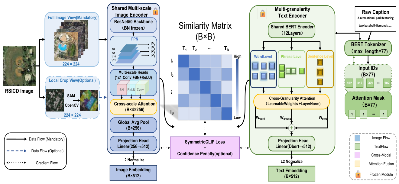
Figure 2.
Multi-granularity text encoder with word-level, phrase-level, and sentence-level branches.
Figure 2.
Multi-granularity text encoder with word-level, phrase-level, and sentence-level branches.
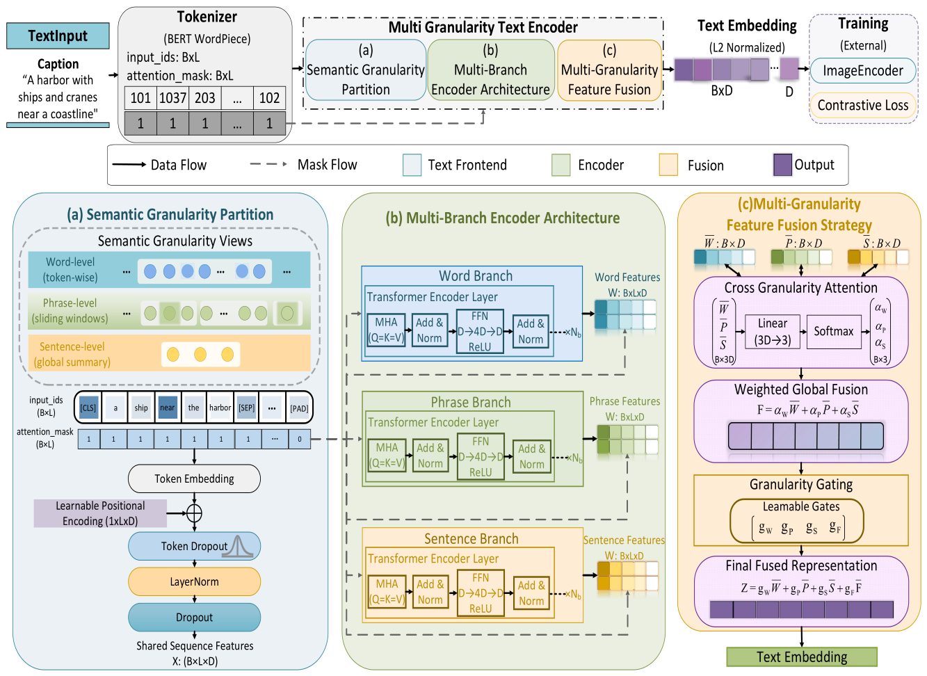
Figure 3.
Scale-aware visual encoder and SAM-guided local-view augmentation.
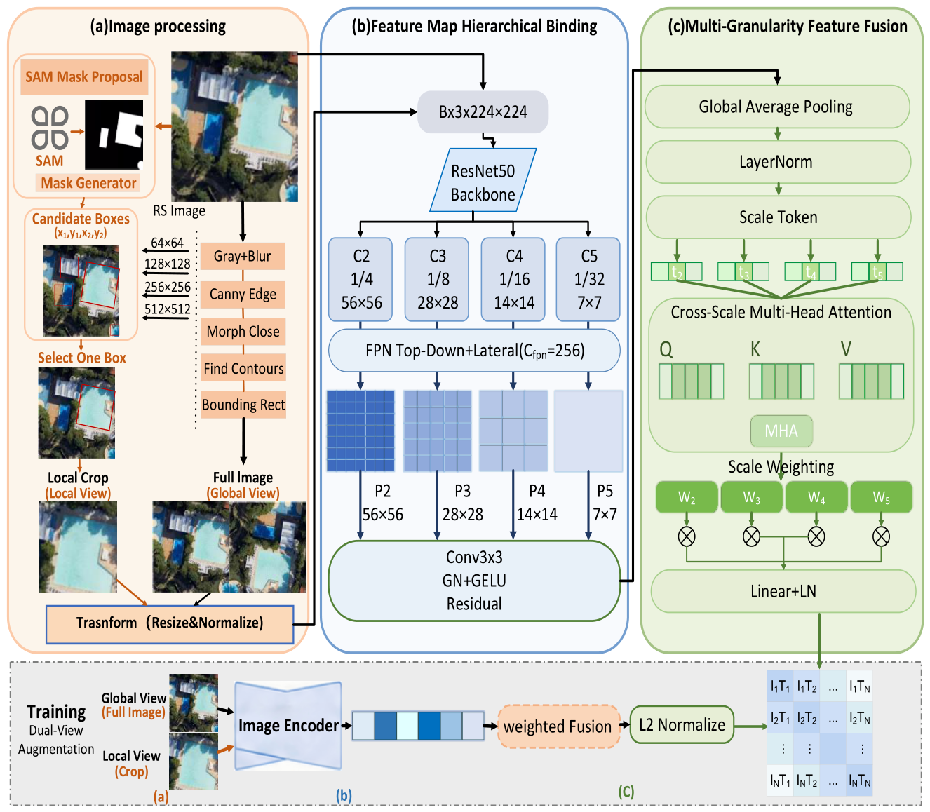
Table 1.
Positioning of the proposed method relative to representative prior work.
| Prior work type | Representative methods | Difference in this work |
| CLIP adaptation | CLIP-Adapter, PE-RSITR | structural encoder adaptation, not adapter/prompt tuning |
| Multi-scale VLM | FPN-style fusion | level descriptors interact via self-attention and gated concatenation |
| Region-level alignment | ViLBERT, UNITER | no detector, no region annotation; SAM provides unsupervised local views |
| Domain-pretrained RS VLM | RemoteCLIP, GeoRSCLIP | no large-scale domain re-pretraining |
| Hard-negative contrastive learning | OHEM, soft contrastive | detached membership weights, bounded discount |
Table 2.
Prompt Sensitivity Analysis.
| Prompt Setting | Templates | Example | mAP (raw class names) | mAP (normalized class names) |
| Bare class name | 1 | storagetanks | 76.4 | 78.3 |
| Generic template | 1 | a photo of storagetanks | 66.5 | 70.3 |
| Remote-sensing template | 1 | a satellite image of storagetanks | 70.8 | 72.1 |
| Five-template ensemble | 5 | …… | 83.6 | 87.5 |
| Attribute-enhanced long prompt | 3 | a high resolution satellite ... | 56.9 | 58.8 |
Table 3.
Scene recognition performance comparison on the RSICD dataset. ( Params refer to trainable parameters of the dual-encoder framework only; SAM is frozen and used only during training/validation as an offline local-view generator.).
Table 3.
Scene recognition performance comparison on the RSICD dataset. ( Params refer to trainable parameters of the dual-encoder framework only; SAM is frozen and used only during training/validation as an offline local-view generator.).
| Method | mAP | Top-1 | Top-2 | Top-3 | Params | Time |
| CLIP[3] | 74.8 | 65.2 | 83.6 | 89.1 | ~151M | 1.5h |
| ViLT[10] | 77.2 | 68.4 | 85.3 | 90.5 | ~111M | 1.17h |
| ALBEF[11] | 79.5 | 71.6 | 87.2 | 91.8 | ~210M | 1.83h |
| BLIP[12] | 81.3 | 73.8 | 88.5 | 92.6 | ~225M | 2.08h |
| Ours | 87.5 | 78.3 | 91.4 | 93.5 | ~59.7M | 1.88h |
Table 4.
Scene recognition performance comparison on the remote sensing scene adaptation dataset. ( Params refer to trainable parameters of the dual-encoder framework only; SAM is frozen and used only during training/validation as an offline local-view generator.).
Table 4.
Scene recognition performance comparison on the remote sensing scene adaptation dataset. ( Params refer to trainable parameters of the dual-encoder framework only; SAM is frozen and used only during training/validation as an offline local-view generator.).
| Method | mAP | Top-1 | Top-2 | Params | Time |
| CLIP[3] | 73.8 | 66.4 | 82.7 | ~151M | 2.18h |
| ViLT[10] | 76.5 | 67.8 | 84.2 | ~111M | 1.7h |
| ALBEF[11] | 78.9 | 70.3 | 85.7 | ~210M | 2.68h |
| BLIP[12] | 82.4 | 73.5 | 87.9 | ~225M | 3.05h |
| Ours | 88.2 | 78.5 | 92.1 | ~59.7M | 2.75h |
Table 6.
Ablation study results of different components.
| Method |
Multi-granularity Semantic |
Scale-aware Visual |
Membership-aware Contrastive |
mAP | Top-1 |
| A | ✗ | ✓ | ✓ | 80.7 | 73.1 |
| B | ✓ | ✗ | ✓ | 81.2 | 74.5 |
| C | ✓ | ✓ | ✗ | 79.7 | 73.7 |
| D(Full) | ✓ | ✓ | ✓ | 87.5 | 78.3 |
Table 7.
Supplementary Ablation on Membership Variants.
| Setting | Top-1 | mAP |
| Detached (Ours default) | 78.3 | 87.5 |
| Standard InfoNCE (w/o membership) | 73.7 | 79.7 |
| Dynamic (gradient flows) | 69.8 | 72.9 |
| Fixed (scene labels) | 77.6 | 85.7 |
Table 8.
Ablation on SAM-guided local-view augmentation on RSICD.
| Setting | Top-1 | mAP |
| w/ SAM (Ours default) | 78.3 | 87.5 |
| w/o SAM | 77.4 | 83.3 |
Disclaimer/Publisher’s Note: The statements, opinions and data contained in all publications are solely those of the individual author(s) and contributor(s) and not of MDPI and/or the editor(s). MDPI and/or the editor(s) disclaim responsibility for any injury to people or property resulting from any ideas, methods, instructions or products referred to in the content. |
© 2026 by the authors. Licensee MDPI, Basel, Switzerland. This article is an open access article distributed under the terms and conditions of the Creative Commons Attribution (CC BY) license (http://creativecommons.org/licenses/by/4.0/).
Copyright: This open access article is published under a Creative Commons CC BY 4.0 license, which permit the free download, distribution, and reuse, provided that the author and preprint are cited in any reuse.