
Submitted:
22 September 2026
Posted:
23 September 2026
You are already at the latest version
Abstract
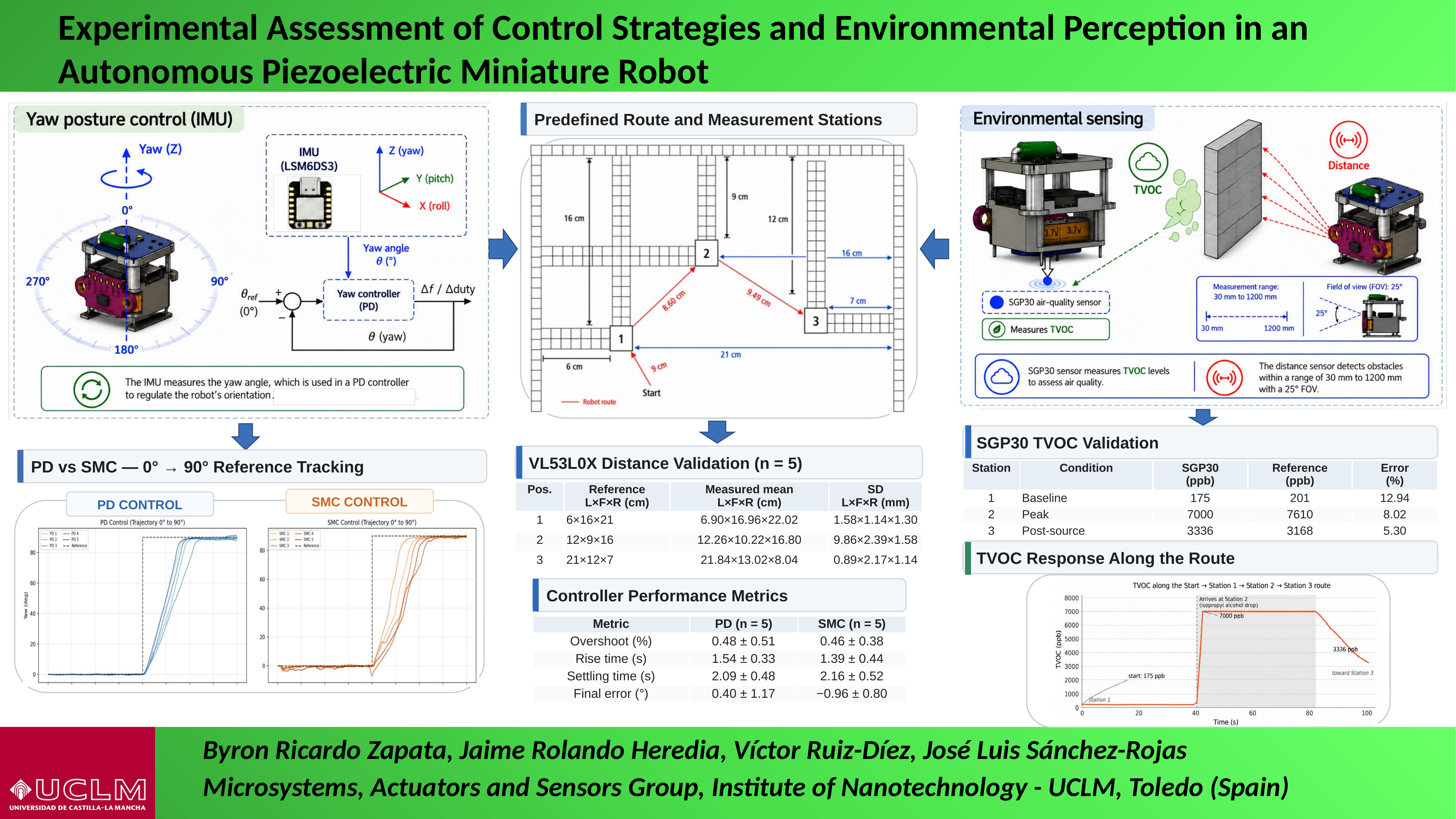
This work presents the functional enhancement of a previously developed miniature robot actuated by 3D-printed piezoelectric resonators through the integration of environmental and spatial sensors and the experimental comparison of proportional–derivative (PD) and sliding mode control (SMC) control strategies. The platform integrates an inertial measurement unit, a time-of-flight distance sensor, and a total volatile organic compound (TVOC) sensor, enabling the robot to execute a predefined route while acquiring environmental and spatial information. Two control strategies, PD and SMC, were experimentally compared using yaw-angle feedback and differential adjustment of the excitation frequencies. For a 0° reference, the PD and SMC controllers achieved mean absolute errors of 0.515° and 0.652°, respectively. During a transition from 0° to 90°, both controllers exhibited similar transient responses; however, during the return transition from 90° to 0°, only the PD controller successfully completed the rotation. In addition, the PD controller achieved a 12.27% higher linear velocity and a 5.44% higher counterclockwise angular velocity. The VL53L0X sensor exhibited a mean absolute error of 0.90 cm and a mean percentage error of 8.22%, while the SGP30 successfully detected the increase in TVOC caused by isopropyl alcohol, with relative differences ranging from 5.30% to 12.94% compared with a low-cost commercial air-quality monitor.
Keywords:
piezoelectric microrobot
; standing-wave locomotion
; piezoelectric actuation
; embedded control
; trajectory control
; autonomous navigation
; environmental sensing
; TVOC detection
; additive manufacturing
1. Introduction
Robotics has progressively evolved from large-scale industrial systems toward increasingly compact, autonomous, and bioinspired platforms. Within this trend, insect-scale miniature robots have attracted growing interest because of their potential ability to operate in confined or difficult-to-access environments. These characteristics make them promising alternatives for applications such as inspection, micromanipulation, minimally invasive medicine, and infrastructure assessment [1,2,3,4,5].
One of the main challenges in the development of these systems lies in the selection of actuators capable of generating efficient, precise, and controllable motion at small scales. In this context, piezoelectric actuators represent a particularly attractive alternative due to their low power consumption, fast dynamic response, high resolution, ease of miniaturization, and robustness against electromagnetic interference [6]. Furthermore, the integration of piezoelectric patches with structures fabricated by 3D printing facilitates mechanical and electronic integration, supporting the development of compact robotic systems.
Several studies have demonstrated the potential of piezoelectric vibrations for generating locomotion in miniaturized robotic systems [7]. The main approaches reported include vibration-driven propulsion in insect-scale robots [8], millimeter-scale omnidirectional platforms [9], dual-beam robots actuated through the simultaneous excitation of vibration modes [10], and three-degree-of-freedom spatial mechanisms based on the stick-slip principle [11]. Comparative studies of locomotion based on traveling and standing waves in bipedal piezoelectric robots have also been reported [12], along with bidirectional ultrasonic motors based on standing waves [13] and bioinspired robots capable of locomotion through traveling waves [14].
More recently, research has shifted toward platforms with higher levels of autonomy and functional integration. In this area, planar piezoelectric resonators have been developed for autonomous miniature robots [15], along with piezoelectrically actuated microminiature crawling robots [16] and lightweight autonomous walking platforms driven by piezoelectric actuators [17]. In parallel, recent reviews have highlighted the increasing use of piezoelectric materials in microrobotic systems and their potential for the development of compact platforms integrating actuation, sensing, and control capabilities [7].
Despite these advances in locomotion mechanisms, many microrobots continue to exhibit limitations related to energy autonomy, environmental perception, and precise trajectory control. However, the progressive miniaturization of circuits for sensing, control, power conditioning, and telemetry, together with the increasing processing capabilities of microcontrollers, has enabled the incorporation of more sophisticated control strategies and expanded the functional capabilities of these platforms. In this context, the development of compact, low-power microcontrollers [18,19], as well as miniaturized digital sensors that are easy to integrate, has facilitated the implementation of embedded electronic systems in millimeter-scale robots.
The incorporation of these technologies has improved both the autonomy and the navigation and control capabilities of microrobots. Insect-scale locomotion systems with energy and control autonomy have been reported [15,20], as well as fully untethered soft [21] and rigid [22] robots capable of autonomous locomotion. In parallel, control strategies have been proposed to improve trajectory-tracking accuracy in 3D-printed piezoelectric microrobots [23], together with electrostatic adhesion mechanisms that enhance maneuverability and trajectory control in insect-scale soft robots [24]. Collectively, these advances demonstrate that the integration of sensing, processing, communication, and control is a fundamental factor in increasing the functional autonomy of microrobots and remains an active and rapidly evolving research area [25].
Consequently, the integration of sensors and embedded electronic systems has become a key factor in improving autonomous navigation, closed-loop control, and environmental information acquisition in small-scale robotic platforms. In this context, the present work extends the functional capabilities of a previously developed miniature robot [23] through the integration of sensors for spatial and environmental data acquisition and the implementation of an additional control strategy. Compared with our previous work [23], which focused on embedded trajectory control using a PD controller and IMU feedback, the main contributions of the present study are: (i) the integration of a VL53L0X time-of-flight sensor and an SGP30 air-quality sensor for onboard spatial and environmental sensing; (ii) the implementation and experimental comparison of sliding mode control (SMC) with the previously implemented PD controller under constant and changing angular references; and (iii) the experimental evaluation of the combined control and sensing capabilities of the robot along a predefined route comprising three measurement stations. These extensions enable the evaluation of the robot’s trajectory-tracking performance under reference changes, as well as its capability to acquire environmental and spatial information while following a predefined route.
2. Materials and Methods
The methodology for the development of this work is divided into six main parts, which are illustrated in Figure 1.
- 3D-piezo actuators: These elements are responsible for generating the robot’s motion. They are fabricated using 3D printing with Formlabs Rigid 10K resin and incorporate strategically placed PZT patches to generate standing waves (SW).
- Electronic components: The robot integrates onboard electronics consisting of batteries, a microcontroller, inertial sensors (IMU), an air quality sensor, a distance sensor, and a power board.
- System integration: The system is integrated by mounting the electronic components and piezoelectric actuators within a structural housing. The housing provides mechanical support and ensures the proper arrangement of the electronic components while also enabling the secure attachment of the piezoelectric actuators that generate the robot’s motion.
- Trajectory control: To ensure proper robot displacement, a control stage is implemented to maintain the robot along a predefined trajectory.
- Environmental signals: The integrated sensors acquire signals related to air quality and distance, which are transmitted and visualized on a computer through a telemetry stage.
- Environmental exploration and signal detection: During a programmed and controlled route, the robot explores its surroundings and collects data using IMU, distance, and air-quality sensors, enabling it to detect obstacles and monitor environmental conditions along its trajectory.
2.1. 3D-piezo Actuator
Piezoelectric actuators are used to generate linear and rotational motion through vibrations induced by standing waves (SW). The piezoelectric elements used in this study are lead zirconate titanate (PZT) patches, specifically the PIC 255 model manufactured by PI Ceramic [11]. These patches are mounted on legged plates designed using CAD software and fabricated from rigid resin using a Formlabs Form 3 stereolithography 3D printer. Both the design and the operating principle of these actuators were previously investigated and validated in [23,26]. Figure 2 shows the piezoelectric actuators A and B used in this work.
The design and manufacturing dimensions of Plates A and B are detailed in Table 1.
For robot motion control and environmental data acquisition, three primary movements are considered: forward motion, clockwise rotation, and counterclockwise rotation. Direct backward motion is not implemented, as the required changes in direction are achieved through differential control of the speed of each piezoelectric actuator. These movements are generated by exciting the (50) mode. Figure 3 shows the deformation of the plates and their legs associated with this vibration mode, obtained from a finite element modal analysis performed using COMSOL Multiphysics.
In this design, the legs associated with plates A and B are strategically positioned between a node and an antinode, within the lobes corresponding to the blue region of the SW wave. Due to the vibrational deformation generated at these points, the free end of each leg undergoes an oscillatory motion along a predominantly diagonal trajectory. When the leg comes into contact with the surface during the downward phase, the horizontal component of this motion generates a frictional and propulsive force, producing rightward displacement. The repetition of this cycle at the excitation frequency allows the vibration of the piezoelectric plates to be transformed into continuous forward motion. The described motions are illustrated in Figure 4.
2.2. Electronic Components
The onboard electronics of the miniature robot consist of the following subsystems: power supply and regulation, control, sensing, and a power stage for the piezoelectric actuators, as shown in Figure 5.
Power supply and regulation: To power the robot and ensure autonomous operation, two 3.7 V Li-Po batteries (401010) are connected in series to provide a total voltage of 7.4 V. This voltage is used to supply the power circuit and, through an AMS1117-3.3 voltage regulator, to power the microcontroller and sensors.
Control stage: Central processing, sensor signal acquisition, and actuator control signal generation are performed by a Seeed Studio XIAO nRF52840 Sense microcontroller. This device integrates a 6-axis IMU comprising a three-axis accelerometer and a three-axis gyroscope, and provides UART, , SPI, SWD, NFC, and Bluetooth 5.0 communication interfaces. The microcontroller measures 21 × 17.5 mm and weighs approximately 3.5 g [27].
Sensing: The robot integrates a VL53L0X time-of-flight (ToF) distance sensor and an SGP30 air-quality sensor for environmental perception. Both devices communicate with the microcontroller through an bus. In addition, the Seeed Studio XIAO board incorporates an IMU used for angular-motion sensing and yaw estimation.
PZT power stage: The piezoelectric actuators are excited by means of an LC resonant circuit, in which each inductor (L1, L2) forms a resonant tank with the intrinsic capacitance of its corresponding piezoelectric plate (PZT_Plate_A, PZT_Plate_B), thereby generating the high-amplitude alternating voltage required to drive the actuators. Switching in each branch is performed by a transistor (Q1A, Q1B), whose base is driven by control signals A and B from the microcontroller through current-limiting resistors (R1, R2). Diodes D1 and D2 protect the transistors against reverse overvoltages generated during switching transients. All circuit references are connected to a common ground (GNDREF).
2.2.1. PZT Power Stage
For the power stage of the PZT actuators, an LC resonant circuit was implemented to increase the excitation voltage applied to the piezoelectric plates. The circuit is driven by a square-wave signal with an amplitude ranging from 0 to 3.3 V and an operating frequency between 58 and 65 kHz, corresponding to the frequency range used to excite (50) mode.
The excitation frequencies were experimentally determined by analyzing the conductance of the piezoelectric plates installed in actuators A and B as a function of frequency, while accounting for the influence of the mechanical and electronic components integrated into the robot’s final configuration. These measurements were performed using a Digilent Analog Discovery 2. Figure 6 shows the resulting conductance curves, from which the resonance frequencies subsequently used to drive the piezoelectric actuators were identified.
The inductors and of the LC resonant circuit, previously shown in Figure 5, are determined using the analysis described in [23]. To obtain an appropriate inductor value () that provides the maximum excitation amplitude at a frequency of 65 kHz, Equation 1 is used, enabling proper impedance matching and efficient resonance.
Where n represents the ratio between the electrical resonance frequency of the LC circuit and the modal resonance frequency of the piezoelectric actuator; is the modal resonance frequency of the selected operating mode; and represents the capacitance of the piezoelectric plates. In this study, was set to , corresponding to the average value obtained from capacitance measurements performed using a Digilent Analog Discovery 2.
Given that bidirectional locomotion requires two distinct excitation frequencies within the (50) mode ( and ), a common nominal inductance value was selected for both resonant branches. Using the relationship , two scenarios arise:
- If the is selected for , then for that frequency and for .
- If the is selected for , then for that frequency and for .
Given that both resulting values remain close to , this integer multiple was selected because it allows for the proper excitation of both frequencies with a single shared inductor, keeping the design close to the maximum power transfer condition previously identified for this drive circuit [23].
Using the defined values and applying Equation 1, an value of is obtained. However, due to commercial availability, a standard value of was selected. The circuit response obtained with this inductance value is shown in Figure 7. The measurements were performed using a 3.3 V input signal while varying the excitation frequency from 58 to 65 kHz and maintaining a fixed 50% duty cycle. This duty cycle was used as an illustrative condition to obtain the voltage response curves. The waveforms were acquired using a Siglent SDS1104X-E digital oscilloscope.
The and values are presented in Table 2. It can be observed that reaches its minimum value of at frequencies between 61 and and then increases again from , reaching at . Meanwhile, the current exhibits only small variations over the range, remaining between and .
2.3. System Integration
The sensors, microcontroller, batteries, and power circuit are integrated into a custom-designed structure developed to minimize the overall dimensions and mass of the robot while providing adequate support for the electronic components. The mass, dimensions, and quantity of the integrated components are detailed in Table 3. These parameters were taken into account during the structural design process to achieve a compact configuration and ensure an appropriate distribution of the components within the available space.
The structure was fabricated using 3D printing with a Formlabs Form 3 printer and Clear Resin, selected for its mechanical properties and its ability to provide sufficiently rigid support for the onboard electronics. Prior to fabrication, the design was evaluated in [23] to verify its ability to withstand the loads associated with the integrated electronic components. Figure 8 shows the structure and its corresponding dimensions.
Figure 9 shows the final implementation of the miniature robot with all electronic, sensing, and actuation components integrated into the 3D-printed structure. The assembled robot has overall dimensions of 26 mm in height, measured from the ground-contact surface to the uppermost point of the inductor, 27 mm in width, and 26 mm in length, with a total mass of 12 g, including the structure and plates A and B.
The pillars connecting plates A and B to the robot structure are strategically positioned at two nodes of the standing wave, located 1.3 mm from the left and right edges, respectively. Each pillar has a diameter of 0.6 mm and a height of 2.8 mm. This placement prevents the pillars from undergoing coupled resonance with the plates, ensuring that the supporting structure does not interfere with the vibration mode of the piezoelectric actuator. The influence of the pillars on the modal response of the plates was evaluated through finite element simulations, and the corresponding results are presented in Figure 10.
The incorporation of the supports resulted in a slight shift in the frequency associated with (50) mode. For plate A, the frequency increased from 53.264 to 53.933 kHz, corresponding to a variation of 1.26%, whereas for plate B, it increased from 57.548 to 58.046 kHz, equivalent to a variation of 0.87%, compared with the results presented in Figure 3. Despite these frequency shifts, the characteristic mode shape remained essentially unchanged, with no significant alterations observed.
2.4. Trajectory control
The trajectory control system is designed to generate controlled movements that enable the robot to explore its environment and collect air-quality data using the onboard sensors. To accomplish this, a predefined path is established for the robot to follow autonomously while minimizing the trajectory-tracking error during motion.
For trajectory tracking, two control strategies are implemented and compared: a proportional-derivative (PD) controller and sliding mode control (SMC). This comparison is used to determine which strategy provides better performance based on tracking metrics and the limitations imposed by the robot’s scale and dynamic characteristics. Figure 11 shows the common block diagram used to implement the control strategies evaluated in this study.
The block diagram in Figure 11 describes the closed-loop control system used to maintain the robot’s trajectory, organized into four stages: (1) reference generation and error calculation, (2) control and excitation signal generation, (3) robot and actuator dynamics, and (4) measurement and feedback signal filtering.
- References and error stage: A reference angle value is defined, which the robot must maintain during its motion. This value is compared with the estimated current angle , obtained in the measurement stage, to calculate the error signal .
- Control and signal generation stage: The error signal is sent to the controller, which calculates the correction signal required to reduce the error. Since does not have a defined limit, this signal is constrained by a frequency saturator, which generates the limited signal , keeping the excitation frequency within the range of (50) mode. This signal is converted into a PWM signal that drives the LC resonant power circuit, generating the excitation voltage applied to the piezoelectric actuators.
- Robot and actuators stage: The voltage excites the piezoelectric actuators, producing the robot’s motion dynamics.
- Measurement and signal filtering stage: The IMU sensor integrated into the robot acquires the angular velocity along the Z-axis, , corresponding to the robot’s rotation about its vertical axis. The reference coordinate system is defined with respect to the board: the X-axis points toward the USB connector, the Y-axis points to the left (with the USB connector on the right), and the Z-axis is perpendicular to the board, pointing outward; the components , , correspond to the linear acceleration along each axis, and , , to the angular velocity, with the positive sign defined according to the right-hand rule. This signal exhibits unwanted peaks produced by the robot’s inherent vibration during motion, which are filtered using a Kalman filter designed to reduce the sensor measurement error and estimate the current angle , which is fed back to the References and error stage to close the control loop [23].
2.4.1. Proportional-Derivative (PD) Control
The controller design is based on [23,28]. The fundamental principle of the controller is to reduce the error between the reference and the robot position by generating a control signal , according to the discretized control law shown in Equation 2:
Where:
- : proportional gain, which enables the system to approach the reference and reduce the error .
- : derivative gain, which helps reduce system oscillations.
- : sampling period, which represents the data acquisition interval.
Since the robot has two actuators, A and B, the following function is defined to generate motion, where represents the excitation frequency generated at a duty cycle, experimentally determined to produce straight-line motion when applied simultaneously to both plates A and B. The controller output is first limited to a maximum deviation of from this baseline, as expressed in Equation 3:
Next, the saturated correction is applied with opposite signs to each actuator, producing a symmetric differential excitation around the 61 kHz baseline, as shown in Equation 4:
This configuration keeps both actuator frequencies within the 58–64 kHz range, corresponding to a symmetric deviation of up to 3 kHz on either side of the resonance peak identified in Figure 6, where (50) mode reaches its maximum electromechanical response for plates A and B. Since shifting away from this peak in either direction produces an equivalent reduction in excitation amplitude, this symmetric formulation makes it possible to selectively weaken either actuator relative to the other, thereby generating the differential thrust required for clockwise and counterclockwise rotation.
The gains and of the PD controller were empirically tuned through a heuristic and iterative process, with the objective of achieving a balance between fast tracking response and closed-loop system stability. To determine , its value was progressively increased until was reached, at which point the controller exhibited a sufficiently fast response for reference tracking. Subsequently, the derivative gain was adjusted until was obtained, with the purpose of damping the resulting oscillations and limiting overshoot during the transient response. The sampling period was set to , corresponding to the execution interval of the sensing-control-actuation cycle. This value represents the discrete interval at which the controller updates the control signal based on the information provided by the measurement system. Therefore, by substituting the tuned values , , and into Equation 2, the following expression is obtained:
2.4.2. Sliding Mode Control
Unlike the PD controller, sliding mode control (SMC) is characterized by its robustness against model uncertainties, external disturbances, and system nonlinearities. Its operating principle consists of forcing the system state to converge toward a sliding surface defined as a function of the angular error and, subsequently, maintaining the system dynamics on this surface [28,29,30].
The SMC control law consists of two terms: a continuous component that acts as a function of the tracking error and a discontinuous component that drives the system toward the sliding surface , keeping it in its vicinity during trajectory tracking. The control law is expressed as:
The saturation function is defined as:
The values used are , , and . The parameter defines the thickness of the boundary layer around the sliding surface. These values were obtained heuristically after conducting different tests of the controller applied to the robot. The use of the saturation function, instead of an ideal sign function, smooths the discontinuous control action and reduces the chattering phenomenon characteristic of sliding mode controllers.
The sliding surface is defined as:
Where is a positive parameter, tuned using the same experimental procedure employed for the previous gains, that determines the convergence dynamics of the error toward the sliding surface, while represents the time derivative of the angular error.
As in the PD controller, the orientation error is defined as . Because the reference is implemented as a sequence of values that remain constant over specific intervals, its derivative is zero while the system operates at the same setpoint, i.e., . Differentiating and substituting into the error function yields:
The derivative of the yaw angle corresponds to the angular velocity about the Z-axis, which is obtained directly from the IMU gyroscope. Therefore:
This formulation allows the angular velocity measurement provided by the IMU to be used directly, avoiding the need to numerically compute the derivative of the orientation angle. In this way, the amplification of noise associated with numerical differentiation is reduced, and a more suitable estimate of the time variation of the error is obtained for implementation of the SMC controller.
The SMC control signal is applied to the piezoelectric actuators through a saturator that limits its maximum deviation with respect to the 61000 Hz baseline, as expressed in Equation 11:
3. Environmental Signals
For the acquisition of environmental variables, two independent sensors were integrated, both communicating with the Seeed Studio XIAO nRF52840 Sense microcontroller through the same bus: a VL53L0X time-of-flight (ToF) distance sensor with address 0x29, and an SGP30 air-quality sensor with address 0x58. These devices were strategically positioned at the front and bottom of the robot, respectively, to enhance its ability to interact with and perceive the surrounding environment. Because both sensors share the same bus, they communicate independently through their respective addresses, allowing sequential data acquisition without interference between devices.
The VL53L0X sensor is used to detect, in real time, obstacles that may interfere with the robot’s motion, providing distance information useful for navigation and collision avoidance. The SGP30 sensor, in turn, is used to monitor air quality by measuring total volatile organic compounds (TVOCs), enabling the detection of potentially abnormal concentrations associated with the presence of volatile substances as the robot travels along a predefined trajectory. Figure 12 shows the physical location of both sensors within the robot structure, together with their main measurement characteristics [31,32].
For the estimation of volatile organic compounds, the SGP30 sensor employs a sensing element based on metal-oxide (MOX) technology, whose electrical conductivity varies as a result of the interaction between gas molecules and the material surface. In general, the behavior of this type of sensor can be represented by a power-law relationship between the resistance of the sensing element and the gas concentration, as expressed in Equation 12:
Where represents the resistance of the sensing element, C corresponds to the gas concentration, A is a proportionality constant, and represents a coefficient associated with the sensitivity of the material. This expression provides a general representation of the behavior of metal-oxide-based sensors and does not directly correspond to the internal algorithm implemented by the manufacturer.
Based on the variations produced in the sensing element, the SGP30 internally performs signal conditioning and processing to provide a digital estimate of the total volatile organic compound (TVOC) concentration, expressed in parts per billion (ppb). Conceptually, this estimate can be represented as a function of the ratio between the instantaneous sensor resistance and a reference value associated with its baseline , according to Equation 13:
The use of a baseline makes it possible to account for temporal variations in the sensing element and improve the stability of the estimate during sensor operation. In the developed system, the measurements provided by the SGP30 are used to identify variations in TVOC levels as the robot moves along a predefined trajectory. To evaluate this capability, the presence of volatile substances, such as isopropyl alcohol, is considered, since their evaporation produces detectable changes in the sensor response.
Because the response of metal-oxide-based sensors can be influenced by environmental conditions, particularly humidity, the SGP30 allows absolute humidity information to be incorporated to compensate for its response. When this information is available, the influence of humidity on the signal can be represented, in general terms, by a correction relationship such as that given in Equation 14:
Where represents the corrected resistance, corresponds to the absolute humidity of the environment, is a reference humidity value, and represents a compensation coefficient. This correction reduces the influence of environmental variations on the response of the sensing element and improves the consistency of the TVOC estimates obtained during robot operation.
The VL53L0X sensor, in turn, employs ToF technology to determine the distance between the robot and obstacles along its trajectory. The device integrates a vertical-cavity surface-emitting infrared laser source, which emits radiation toward the target, and a single-photon avalanche diode array responsible for detecting the photons reflected from its surface. Based on the time interval elapsed between the emission of the optical signal and the detection of its return, the distance d to the object can be generally represented by Equation 15:
Where c corresponds to the speed of light in vacuum (), and is the time of flight of the optical signal. The factor accounts for the fact that the radiation travels the measured distance twice, first from the sensor to the object and then from the object back to the receiver. The processing required to estimate this distance is performed internally by the VL53L0X, which directly provides the microcontroller with the digital measurement value through the interface.
4. Results
For the experimental evaluation of the miniature robot, the following tests were conducted:
- 1.
- Trajectory control tests, performed to verify the robot’s performance in following a predefined trajectory using closed-loop control.
- 2.
- Reference-change control tests, aimed at comparing the performance of the PD and SMC controllers in response to a change in angular reference.
- 3.
- Distance measurement verification, conducted to validate the accuracy of the VL53L0X sensor.
- 4.
- TVOC measurements, performed to evaluate the ability of the SGP30 sensor to detect variations in air quality during the robot’s motion.
These tests provide the basis for evaluating the robot’s performance under the SMC and PD trajectory control strategies, its tracking capability in response to changes in the reference trajectory, and the acquisition of environmental variables, specifically distance and TVOC concentration. The results obtained for each control strategy and experimental test are presented and analyzed in the following subsections.
4.1. Closed-Loop Trajectory Control with a 0° Reference
This test evaluates the closed-loop response of the PD and SMC controllers under a constant angular reference of 0°, corresponding to the robot’s straight-line motion. Five repetitions were performed for each control strategy, with a duration of 7 s per trial. During each test, the robot’s angular position about the Z-axis (yaw) was recorded and transmitted in real time via Bluetooth. The interface was used exclusively for signal acquisition and recording and therefore did not interfere with motion generation or the control action. Figure 13 presents the responses obtained for both control strategies.
Table 4 presents the mean absolute error, standard deviation, and maximum peak metrics obtained from the five tests performed with each controller. Both controllers exhibit very similar mean absolute error values, indicating comparable performance in tracking the angular reference. However, the SMC controller shows a higher standard deviation and a larger maximum peak, with values of and , respectively, compared with and obtained with the PD controller. This behavior is mainly associated with the initial transient corresponding to the reaching phase characteristic of sliding mode control, as observed in Figure 13.
4.2. Closed-Loop Trajectory Control with a Reference Change from 0° to 90°
This test evaluates the tracking capability of the PD and SMC control strategies in response to an angular reference change from 0° to 90°. During the first 10 s, the reference was maintained at 0°, corresponding to the robot’s straight-line motion. Subsequently, between 10 and 20 s, the reference was changed to 90°, producing a counterclockwise rotation until the new reference was reached. Five repetitions were performed for each control strategy under the same experimental conditions.
Figure 14 presents the robot’s angular response obtained with both control strategies, together with the corresponding control signals represented by the excitation frequencies applied to actuators A and B. These results allow the transient behavior, tracking speed, reference error, and evolution of the control signals during the change in orientation to be compared.
Table 5 presents the overshoot, rise time, settling time, and final error values obtained with both controllers in response to a reference change. These results show that the overshoot, rise time, and settling time metrics are similar for both controllers. However, the magnitude of the final error is greater for the SMC controller () than for the PD controller (), indicating that the SMC tends to slightly exceed the reference, whereas the PD tends to remain slightly below it.
4.3. Closed-Loop Trajectory Control with a Reference Change from 0° to 90° and Return to 0°
This test evaluates the robot’s ability to maintain a straight-line trajectory and execute changes in orientation using the PD and SMC control strategies, applied independently. During the first 7 s, the angular reference was maintained at 0°, corresponding to the robot’s straight-line motion. Subsequently, between 7 and 14 s, the reference was changed to 90°, producing a counterclockwise rotation until the new desired orientation was reached. Finally, from 14 s onward, the reference returned to 0°, producing a clockwise rotation until the initial orientation was recovered.
This sequence makes it possible to evaluate the performance of both control strategies under successive reference changes, considering both the response during rotation and the robot’s ability to return to its initial orientation. Figure 15 presents the response obtained with the PD controller during this test.
The results presented in Table 6 show that, during the reference change from to , the controller exhibits a considerably longer fall time and settling time, as well as greater dispersion in the final error, with a value of , compared with obtained during the change from to . This behavior is consistent with the previously reported asymmetry between the robot’s clockwise and counterclockwise rotational motions [23], which is associated with mechanical differences and the resulting dynamic response depending on the direction of rotation.
Figure 16 presents the response of the SMC controller. During the transition from 0° to 90°, the system adequately tracks the reference; however, during the transition from 90° to 0°, it fails to reach the desired value. The control signals exhibit saturation at the established frequency limits, between 58 and 64 kHz, indicating a reduction in control authority during clockwise rotation and limiting the controller’s ability to fully compensate for the tracking error.
Based on the tests presented, it was determined that, during straight-line motion, the robot’s linear velocity with the PD controller was 12.27% higher than that obtained with the SMC controller. During counterclockwise rotation, the PD controller also exhibited better performance, achieving an angular velocity 5.44% higher than that recorded with the SMC controller. In contrast, during clockwise rotation, only the PD controller was able to complete the maneuver, reaching an angular velocity of 7.02°/s, whereas the SMC controller was unable to reverse the direction of rotation in any of the trials performed. The results of the velocity analysis under the different motion conditions are presented in Figure 17.
4.4. Speed and Orientation Control Test with Additional Weight
This test evaluates the performance of the PD and SMC controllers during straight-line motion with an angular reference of 0°, after adding an additional weight of 9.35 g to the robot. This weight consisted of a 1.61 g mounting base and a 7.74 g 50-cent coin. The test was conducted to observe the behavior of both controllers under the increased mass and to determine their ability to maintain the robot’s orientation during motion. Five trials were performed for each control strategy under the same conditions. Figure 18 presents the yaw-angle response obtained with the PD and SMC controllers.
Figure 18 shows that the PD controller maintained the yaw angle close to the 0° reference, with only small variations during motion. The mean absolute error was 0.247°, with a standard deviation of 0.215° and a maximum yaw value of 0.840°. In contrast, the SMC controller exhibited larger oscillations around the reference, with a mean absolute error of 0.922°, a standard deviation of 0.824°, and a maximum value of 1.520°. As shown in Table 7, under these conditions, the PD controller produced smaller variations in the yaw angle and better performance in maintaining a straight trajectory under the increased mass.
4.5. Detection of Environmental and Spatial Signals
Following the analysis of the trajectory control strategies, an experimental route consisting of three measurement stations was defined. At each station, the robot stops to detect volatile compounds and measure the distance to the boundary walls located in front of, to the left of, and to the right of the robot. These tests were carried out within a circuit specifically designed to evaluate the robot’s ability to acquire environmental and spatial information during motion. Figure 19 shows the planned route, the locations of the three measurement stations, and the main dimensions of the circuit.
Table 8 presents the measurements obtained with the VL53L0X sensor at the three defined stations, compared with the reference coordinates determined experimentally. The data recorded by the robot were transmitted in real time to a computer via a Bluetooth communication interface used exclusively for data acquisition and storage. Five measurements were performed at each station. Considering the complete set of measurements, a mean absolute error of 0.90 cm was obtained, corresponding to a mean percentage error of approximately 8.22% relative to the reference values. These results show good agreement between the distances estimated by the robot and the actual dimensions of the experimental environment.
For the acquisition of the TVOC and CO2eq signals on the robot, the following strategies were implemented:
- 1.
- Baseline stabilization: The robot was kept isolated inside a closed enclosure for one hour while continuous measurements were recorded under stationary conditions. During this period, the robot was powered through a USB cable, with the batteries disconnected, in order to avoid voltage fluctuations.
- 2.
- Data storage: The parameters obtained during baseline stabilization were stored in the Flash memory of the Seeed Studio XIAO nRF52840 microcontroller.
- 3.
- Initial warm-up: The micro-hotplate membrane was activated for 15 s before the first movement, from the Start position toward Station 1, in order to allow the sensor to reach its operating thermal regime.
- 4.
- Dosing: At Station 2, a droplet of isopropyl alcohol was placed 2 cm from the sensor.
- 5.
- Purge and stabilization time: A 30 s pause was established at each station to allow partial dissipation of the analyte and stabilization of the sensor reading before the robot continued along the route.
At Station 1, the robot recorded a stable value corresponding to its minimum reference level of , while TVOC showed clean-air baseline values ranging from 121 to , confirming the initial environmental conditions. Upon reaching Station 2, where of isopropyl alcohol () had been deposited at a distance of from the sensor, both signals exhibited a sharp increase. reached a peak of , whereas TVOC reached its maximum reporting limit of , a response consistent with exposure to a high concentration of volatile organic compounds.
The TVOC signal remained saturated for a considerably longer period, approximately , compared with , which remained at its maximum value for approximately . This behavior is attributed to the greater dependence of the TVOC calculation on the ethanol-related signal, whose dissipation is slower than that of the combined signals used for estimation.
As the robot moved toward Station 3, both readings progressively decreased. TVOC dropped to approximately , while decreased to approximately . However, neither signal returned to its baseline within the recording window because of residual alcohol vapor retained by the sensor and dispersed in the immediate surroundings, as shown in Figure 20.
To validate the accuracy of the TVOC measurements obtained with the SGP30 sensor, the test results were compared with readings from a low-cost portable air-quality monitor (Air Quality Monitor Indoor, 10-in-1), used as a commercial reference device. The comparison was performed under the three characteristic conditions of the route: the baseline condition before exposure to the source (Station 1), the point of maximum exposure to isopropyl alcohol (Station 2), and the subsequent dissipation phase (Station 3). The results are summarized in Table 9.
As observed, the relative error remained below 13% under all three evaluated conditions. The closest agreement was obtained at the point of maximum exposure, with an error of 8.02%, and during the dissipation phase, with an error of 5.30%, conditions under which both sensors recorded concentrations substantially above their lower detection limits.
4.6. Energy Consumption and Autonomy
Energy consumption was determined experimentally using a Fluke 177 True RMS digital multimeter to measure the battery voltage and the total current drawn by the electronic system, including the microcontroller, IMU, distance sensor, gas sensor, and actuator drivers. The measurements were performed with fully charged batteries and all sensors active. The instantaneous power consumption was calculated as the product of the measured voltage and current, according to Equation 16:
Where is the battery voltage at full charge, and is the maximum current drawn by the robot during straight-line trajectory tests.
Battery autonomy was determined using a stopwatch by measuring the elapsed time from full charge until the battery voltage dropped below 6.5 V, the threshold below which the robot no longer operated properly. The total operating time was approximately 20 minutes.
5. Discussion
The results obtained show that the functional expansion of the previously developed platform enabled the integration of embedded control and the acquisition of spatial and environmental information while maintaining the operation of the piezoelectric locomotion system. During the experimental tests, the robot achieved, with the PD controller, speeds of up to 16.84 mm/s during straight-line motion and angular velocities of 27.89°/s and 7.02°/s during counterclockwise and clockwise rotations, respectively. The difference observed between the two directions of rotation indicates an asymmetric response of the locomotion system, a behavior that is also reflected in the control tests.
In the comparison of the PD and SMC control strategies, both controllers were able to maintain a 0° angular reference, with mean absolute errors of 0.515° and 0.652°, respectively. During the reference change from 0° to 90°, both exhibited similar behavior; however, during the return from 90° to 0°, only the PD controller was able to complete the rotation, although with greater dispersion in the final error (SD = 5.31°), indicating lower consistency in this direction. The SMC control signals reached the established frequency limits without being able to reverse the direction of rotation. These results suggest that both the mechanical asymmetry of the system and the available excitation-frequency range constrain the actuation capability during clockwise rotation; therefore, this response cannot be attributed solely to the control strategy.
Compared with the previous work developed using the same platform [23], in which trajectory control was implemented using a PD controller with IMU feedback, the present work extends the robot’s functional capabilities through the integration of a VL53L0X distance sensor, an SGP30 TVOC sensor, and the additional implementation of an SMC controller. Thus, in addition to moving and maintaining an orientation reference, the robot is able to acquire spatial and environmental information while following a predefined route.
Table 10 compares these characteristics with those of other miniature robots reported in the literature.
Some studies achieve considerably higher velocities, such as robots based on bimorph actuators with 3D-printed legs [8], BHMbot [22], and HARM-F [20]. However, these platforms are primarily focused on locomotion performance. BHMbot, for example, does not integrate an IMU or environmental sensors, and its operation relies on wireless directional commands rather than closed-loop angular feedback. Similarly, the robot reported by Robles-Cuenca et al. [15], based on piezoelectric resonators, features a compact architecture and energy autonomy but does not incorporate distance or gas sensors. In contrast, more recent platforms exhibit a higher degree of functional integration. The tripod piezoelectric microrobot reported in [36] incorporates control, an IMU, and perception sensors, reflecting a growing trend toward miniature robots with enhanced autonomy and sensing capabilities. The present work follows this same direction within a smaller and lighter platform. Although its velocity does not exceed that of several of the robots included in the comparison, the implemented control system enables the angular tracking error to be quantitatively characterized through repeated experimental trials, a metric that is not reported for the tripod robot considered in the comparison.
Regarding the sensing system, the VL53L0X enabled spatial information acquisition with a mean absolute error of 0.90 cm, corresponding to a mean percentage error of 8.22% relative to the reference distances. The SGP30 successfully detected the increase in TVOC produced by an isopropyl alcohol source, with relative differences ranging from 5.30% to 12.94% compared with the commercial monitor. These results demonstrate that the integration of both sensors is suitable for the intended tasks while preserving the robot’s locomotion and control capabilities.
6. Conclusions
The results obtained indicate that the integration and placement of the VL53L0X and SGP30 sensors on the robot were suitable for the intended functions. These locations enabled the acquisition of spatial and environmental data during the robot’s motion without hindering its displacement or affecting the operation of the control system. In this regard, the results validate the feasibility of incorporating perception sensors into miniature robots driven by piezoelectric actuators while maintaining a compact and functional configuration for supporting the feasibility of the proposed platform for future exploration and inspection applications.
The experimental tests showed that both controllers were capable of maintaining an angular reference of 0°, with mean absolute errors of 0.515° for the PD controller and 0.652° for the SMC controller. However, when reference changes were evaluated, the PD controller exhibited behavior that was better suited to the dynamic characteristics of the robot. In particular, during the return from 90° to 0°, only the PD controller was able to complete the clockwise rotation, whereas the SMC controller reached the established frequency limits and was unable to reverse the direction of motion.
The comparison of the measured velocities showed that the PD controller achieved a 12.27% higher linear velocity than the SMC controller during straight-line motion and a 5.44% higher angular velocity during counterclockwise rotation. For clockwise rotation, the PD controller reached an angular velocity of 7.02°/s, whereas the SMC controller was unable to complete this maneuver in the tests performed. These results highlight the influence of mechanical asymmetry and excitation-frequency limits on the robot’s control capability.
The integration of the VL53L0X and SGP30 sensors enabled the robot to acquire spatial and environmental information while traveling along a route consisting of three stations. For the distance measurements, a mean absolute error of 0.90 cm was obtained, corresponding to a mean percentage error of 8.22% relative to the reference distances. In addition, the SGP30 successfully detected the increase in TVOC caused by the presence of isopropyl alcohol, with relative differences ranging from 5.30% to 12.94% compared with a low-cost commercial monitor. Overall, these results demonstrate the feasibility of integrating trajectory control and environmental data acquisition into a miniature robotic platform driven by piezoelectric actuators.
Supplementary Materials
The following supporting information can be downloaded at the website of this paper posted on Preprints.org:
- Video S1—Experimental evaluation of the PD and SMC controllers. Experimental test of the PD and SMC control strategies for maintaining a 0° angular reference. The video shows the behavior of the miniature robot under both control strategies and their ability to maintain its orientation during straight-line motion. Direct link: https://drive.google.com/file/d/10ZrD_0JXgGkWREgBAPF3G5d2IzjYgjeT/view?usp=drive_link
- Video S2—Response of the PD and SMC controllers to an angular reference change. An experimental test of the PD and SMC control strategies is presented, in which the robot initially maintains a 0° angular reference and subsequently changes to a 90° reference. The video shows the behavior of the robot and the response of both control strategies during the change in orientation. Direct link: https://drive.google.com/file/d/1oyCKfM5BUfqRvWjBbkSBzKZ-YHxj5Muf/view?usp=drive_link
- Video S3 — Response of the PD and SMC controllers with additional weight. An experimental test of the PD and SMC control strategies is presented for maintaining a 0° angular reference after adding an additional weight of 9.35 g to the robot. The video shows the behavior of the robot under both control strategies and their ability to maintain its orientation during straight-line motion with the increased mass. Direct link: https://drive.google.com/file/d/1yFjI0X_3QgPHdKLt3XW2f4c7_srUyh9f/view?usp=drive_link
- Video S4 — Distance and TVOC data acquisition. An experimental test of the robot’s ability to acquire spatial and environmental information during motion is presented. The video shows distance measurements obtained with the VL53L0X sensor and TVOC data acquired with the SGP30 sensor along the trajectory. Direct link: https://drive.google.com/file/d/1Qkjgfg3s7hcffsK27Pn395Y3UJvEAM9D/view?usp=drive_link
Author Contributions
Conceptualization, V.R.-D., and J.L.S.-R.; software B.Z.C. and J.H.V.; investigation, B.Z.C. and J.H.V.; data curation, B.Z.C. and J.H.V.; writing-original draft preparation, B.Z.C. and J.H.V.; writing-review and editing, V.R.-D., and J.L.S.-R.; project administration, V.R.-D., and J.L.S.-R.; funding acquisition, V.R.-D., and J.L.S.-R. All authors have read and agreed to the published version of the manuscript.
Funding
This work was supported by the Universidad de Castilla-La Mancha, Spain, through MCIN/AEI and FEDER "ERDF A way of making Europe" under Grant PID2023-146163OB-I00 and Universidad Politécnica Salesiana, Quito-Ecuador.
Institutional Review Board Statement
Not applicable.
Informed Consent Statement
Not applicable.
Data Availability Statement
The datasets presented in this article are not readily available because the data are part of an ongoing study and due to technical/ time limitations. Requests to access the datasets should be directed to bzapata@ups.edu.ec.
Conflicts of Interest
The authors declare no conflicts of interest. The funders had no role in the design of the study; in the collection, analyses, or interpretation of data; in the writing of the manuscript, or in the decision to publish the results.
References
- Siciliano, B.; Khatib, O. Springer Handbook of Robotics, 2nd ed.; Springer: Cham, Switzerland, 2016.
- Pfeifer, R.; Lungarella, M.; Iida, F. The Challenges Ahead for Bio-Inspired `Soft’ Robotics. Communications of the ACM 2012, 55, 76–87.
- Hammond, M.; Cichella, V.; Lamuta, C. Bioinspired Soft Robotics: State of the Art, Challenges, and Opportunities. Current Robotics Reports 2023, 4, 65–80.
- Zhang, Y.; Li, C.; Chen, X.; Wang, H. Bioinspired Sensors and Applications in Intelligent Robots: A Review. Robotics and Artificial Intelligence 2023, 10, 88–104.
- Bandari, V.K.; Eom, S.H.; Park, H.; Lee, S.W.; Jeong, U. System-Engineered Miniaturized Robots: From Structure to Intelligence. Advanced Intelligent Systems 2021, 3, 2000284.
- Mittal, V.; Singh, R. A Review of Bio-Inspired Actuators and Their Potential for Autonomous Systems. Actuators 2025, 14, 303.
- Fath, A.; Xia, T.; Li, W. Recent Advances in the Application of Piezoelectric Materials in Microrobotic Systems. Micromachines 2022, 13, 1422. [CrossRef]
- Ramírez-Palma, M.R.; Robles-Cuenca, D.; Ruiz-Díez, V.; Hernando-García, J.; Sánchez-Rojas, J.L. Vibration Propulsion in Untethered Insect-Scale Robots. Robotics 2024, 13, 135.
- Kim, H.J.; Kim, S.M.; Kim, H.T.; Yi, B.J. An Omnidirectional Mobile Millimeters Size Micro-Robot. International Journal of Advanced Robotic Systems 2008, 5, 41–46.
- Zhu, B.; Li, C.; Wu, Z.; Li, Y. A Double-Beam Piezoelectric Robot Based on the Principle of Two-Mode Excitation. Sensors and Actuators A: Physical 2024, 369, 115154.
- Wang, Y.; Zhang, L.; Zhao, H.; Li, Y.; Zhao, X. A Spatial 3-DOF Piezoelectric Robot and Its Speed-Up Trajectory Based on Improved Stick-Slip Principle. Mechanical Systems and Signal Processing 2021, 150, 107247.
- Ruiz-Díez, V.; Hernando-García, J.; Toledo, J.; Ababneh, A.; Seidel, H.; Sánchez-Rojas, J.L. Comparative Study of Traveling and Standing Wave-Based Locomotion of Legged Bidirectional Miniature Piezoelectric Robots. Actuators 2021, 10, 136.
- He, S.; Chen, W.; Tao, X.; Chen, Z. Standing Wave Bi-Directional Linearly Moving Ultrasonic Motor. IEEE Transactions on Ultrasonics, Ferroelectrics, and Frequency Control 1998, 45, 1133–1139.
- Wang, Y.; Li, J.; Zhang, S.; Deng, J.; Chen, W.; Liu, Y. A Snail-Inspired Traveling-Wave-Driven Miniature Piezoelectric Robot. Cell Reports Physical Science 2024, 5, 102201.
- Robles-Cuenca, D.; Ramírez-Palma, M.R.; Ruiz-Díez, V.; Hernando-García, J.; Sánchez-Rojas, J.L. Miniature Autonomous Robot Based on Legged In-Plane Piezoelectric Resonators with Onboard Power and Control. Micromachines 2022, 13, 1815.
- Zheng, Z.; Zhao, Y.; Wang, G. Research on Piezoelectric Driving Microminiature Three-Legged Crawling Robot. Journal of Bionic Engineering 2023, 20, 1481–1492. [CrossRef]
- Baisch, A.T.; Heimlich, C.; Karpelson, M.; Wood, R.J. HAMR3: An Autonomous 1.7g Ambulatory Robot. In Proceedings of the 2011 IEEE/RSJ International Conference on Intelligent Robots and Systems (IROS), San Francisco, CA, USA, 2011. [CrossRef]
- Seeed Studio. Seeed Studio XIAO nRF52840 Sense Product Specification v1.5. Technical report, Seeed Studio, Shenzhen, China, 2024. Available online: https://files.seeedstudio.com/wiki/XIAO-BLE/nRF52840_PS_v1.5.pdf (accessed 10 October 2025).
- Rovai, M.J. XIAO: Big Power, Small Board, 2023. GitHub eBook. Available online: https://mjrovai.github.io/XIAO_Big_Power_Small_Board-ebook/ (accessed 10 October 2025).
- Goldberg, B.; Zufferey, R.; Doshi, N.; Helbling, E.F.; Whittredge, G.; Kovac, M.; Wood, R.J. Power and Control Autonomy for High-Speed Locomotion with an Insect-Scale Legged Robot. IEEE Robotics and Automation Letters 2018, 3, 987–993.
- Wu, X.; Cao, L.; Lu, G.; Wang, P.; Ran, L.; Peng, B. Untethered Soft Microrobot Driven by a Single Actuator for Agile Navigations. Nature Communications 2025, 16, 61810.
- Liu, Z.; Zhan, W.; Liu, X.; Zhu, Z.; Qi, M.; Leng, J.; Han, S.; Wu, X.; Yan, X. A Wireless Untethered Robotic Insect with Ultrafast Running Speeds. Nature Communications 2024, 15, 3815.
- Zapata Chancusig, B.R.; Heredia Velastegui, J.R.; Ruiz-Díez, V.; Sánchez-Rojas, J.L. Autonomous Locomotion and Embedded Trajectory Control in Miniature Robots Using Piezoelectric-Actuated 3D-Printed Resonators. Actuators 2026, 15, 23. [CrossRef]
- Liang, W.; Wu, J.; Yim, J.K.; Chen, H.; Miao, Z.; Liu, H.; Liu, Y.; Wang, Y.; Qiu, W. Electrostatic Footpads Enable Agile Insect-Scale Soft Robots with Trajectory Control. Science Robotics 2021, 6, eabe7906. [CrossRef]
- Jiang, J.; Yang, Z.; Ferreira, A.; Zhang, L. Control and Autonomy of Microrobots: Recent Progress and Perspective. Advanced Intelligent Systems 2022, 4, 2100279. [CrossRef]
- Ruiz-Díez, V.; García-Caraballo, J.L.; Hernando-García, J.; Sánchez-Rojas, J.L. 3D-Printed Miniature Robots with Piezoelectric Actuation for Locomotion and Steering Maneuverability Applications. Actuators 2021, 10, 335. [CrossRef]
- Studio, S. XIAO BLE Sense Wiki. https://wiki.seeedstudio.com/XIAO_BLE/, 2025. Accessed: 19 September 2025.
- Ming, M.; Liang, W.; Feng, Z.; Ling, J.; Al Mamun, A.; Xiao, X. PID-Type Sliding Mode-Based Adaptive Motion Control of a 2-DOF Piezoelectric Ultrasonic Motor Driven Stage. Mechatronics 2021, 76, 102543. [CrossRef]
- Zapata, B.; Heredia, J.; Proaño, J. Design and Evaluation of the PID, SMC and MPC Controllers by State Estimation by Kalman Filter in the TRMS System. In Proceedings of the Innovation and Research - A Driving Force for Socio-Econo-Technological Development; Botto-Tobar, M.; Vizuete, M.Z.; Cadena, A.D., Eds., Cham, Switzerland, 2021; Vol. 1277, Advances in Intelligent Systems and Computing, pp. 531–544. [CrossRef]
- Liang, J.; Jing, K.; Dong, Y.; Lin, X.; Wang, Y. Nominal-Model-Based Sliding-Mode Control for Traveling-Wave Ultrasonic Motor. Micromachines 2022, 13, 1846. [CrossRef]
- STMicroelectronics. VL53L0X: World’s Smallest Time-of-Flight Ranging and Gesture Detection Sensor. Technical report, STMicroelectronics, 2021. Datasheet. Available online: https://www.st.com/resource/en/datasheet/vl53l0x.pdf (accessed 19 August 2026).
- Sensirion AG. SGP30: Indoor Air Quality Sensor for TVOC and CO2eq Measurements. Technical report, Sensirion AG, 2020. Datasheet, Version 1.0. Available online: https://sensirion.com/media/documents/984E0DD5/61644B8B/Sensirion_Gas_Sensors_Datasheet_SGP30.pdf (accessed 19 August 2026).
- Ji, X.; Liu, X.; Cacucciolo, V.; Imboden, M.; Civet, Y.; El Haitami, A.; Cantin, S.; Perriard, Y.; Shea, H. An Autonomous Untethered Fast Soft Robotic Insect Driven by Low-Voltage Dielectric Elastomer Actuators. Science Robotics 2019, 4, eaaz6451. [CrossRef]
- Liu, Y.; Chen, Y.; Feng, B.; Wang, D.; Liu, T.; Zhou, H.; Li, H.; Qu, S.; Yang, W. S2worm: A Fast-Moving Untethered Insect-Scale Robot with 2-DoF Transmission Mechanism. IEEE Robotics and Automation Letters 2022, 7, 6758–6765. [CrossRef]
- Johnson, K.; Englhardt, Z.; Arroyos, V.; Yin, D.; Patel, S.; Iyer, V. MilliMobile: An Autonomous Battery-free Wireless Microrobot. In Proceedings of the Proceedings of the 29th Annual International Conference on Mobile Computing and Networking (MobiCom ’23). ACM, 2023, pp. 1–16. [CrossRef]
- Gao, Y.; Li, J.; Zhang, S.; Yan, J.; Zhang, Y.; Liu, B.; Guan, J.; Wang, D.; Deng, J.; Liu, Y. Omnidirectional Motion of an Untethered Tripodal Microrobot Using Radial Piezoelectric Actuators. Nature Communications 2026, 17, 5946. [CrossRef]
Figure 1.
Methodology for the Trajectory Control of a Miniature Robot.
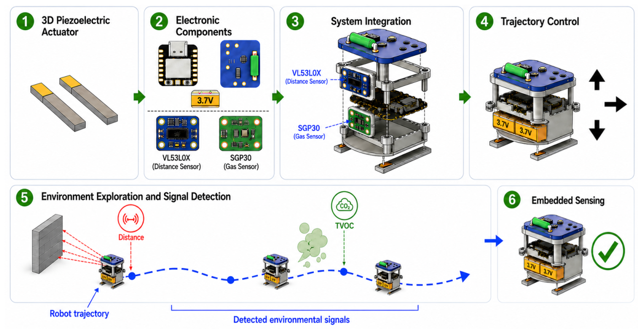
Figure 2.
(a) Plates A and B with PZT patches. (b) Legs (blue parts) on plates A and B for the generation of linear movements.
Figure 2.
(a) Plates A and B with PZT patches. (b) Legs (blue parts) on plates A and B for the generation of linear movements.
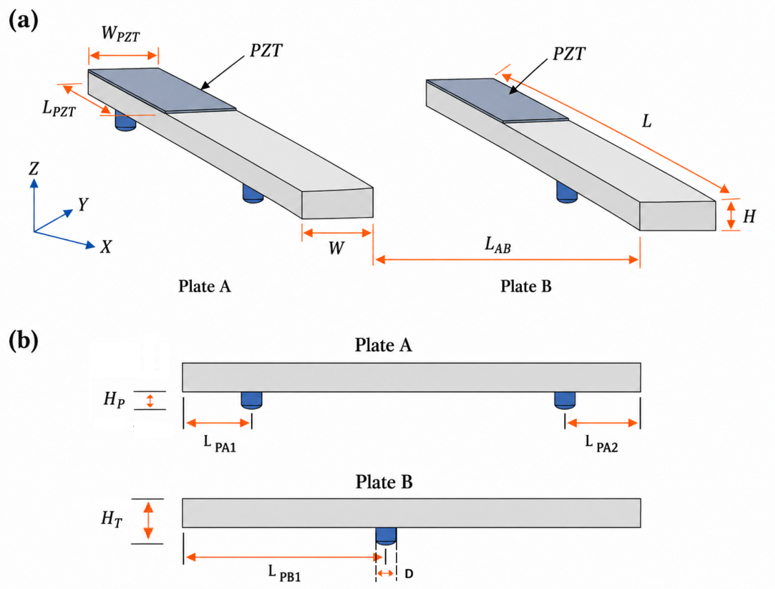
Figure 3.
Vibrational response of Plates A and B under the (50) mode. (a) Deformation and displacement magnitude of Plate A at a frequency of 53.26 kHz; (b) deformation and displacement magnitude of Plate B at its eigenfrequency of 57.54 kHz; and (c) and (d) displacement profiles along the arc length for the Z-component.
Figure 3.
Vibrational response of Plates A and B under the (50) mode. (a) Deformation and displacement magnitude of Plate A at a frequency of 53.26 kHz; (b) deformation and displacement magnitude of Plate B at its eigenfrequency of 57.54 kHz; and (c) and (d) displacement profiles along the arc length for the Z-component.
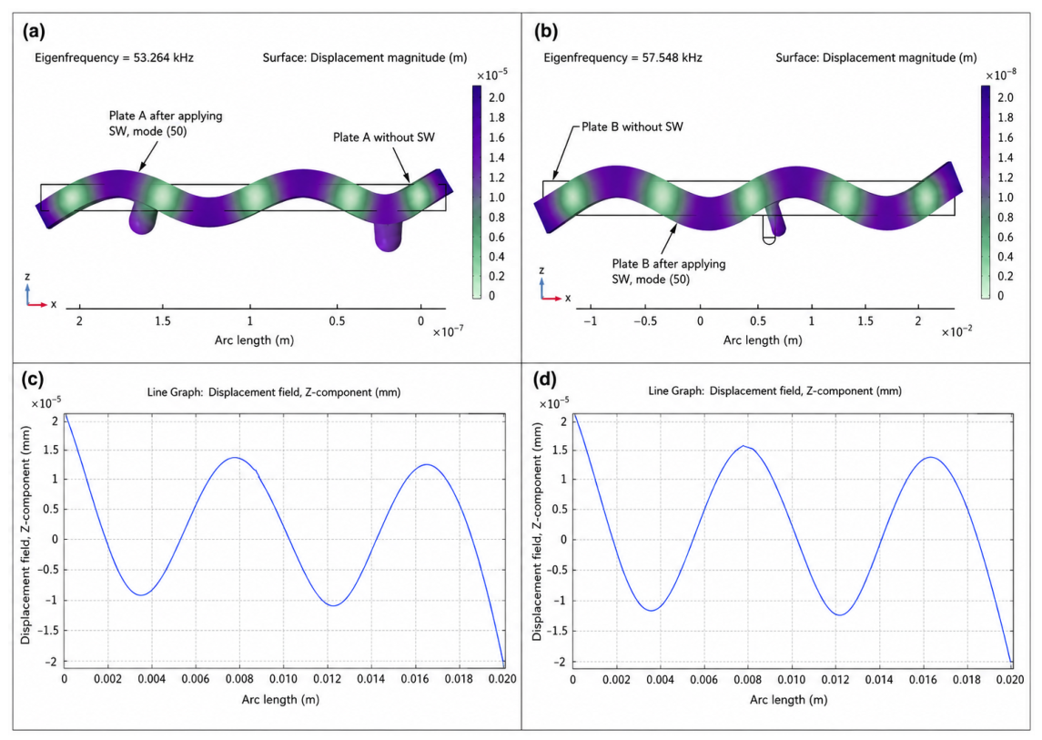
Figure 4.
Generation of the robot’s forward motion through the interaction between the deformation produced by the SW and the legs. (a) Position of the legs associated with plates A and B within the blue regions corresponding to the (50) mode. (b) Diagonal oscillatory motion of the free ends of the legs and generation of a friction-induced propulsive force during contact with the surface. (c) Resulting rightward displacement of plates A and B.
Figure 4.
Generation of the robot’s forward motion through the interaction between the deformation produced by the SW and the legs. (a) Position of the legs associated with plates A and B within the blue regions corresponding to the (50) mode. (b) Diagonal oscillatory motion of the free ends of the legs and generation of a friction-induced propulsive force during contact with the surface. (c) Resulting rightward displacement of plates A and B.
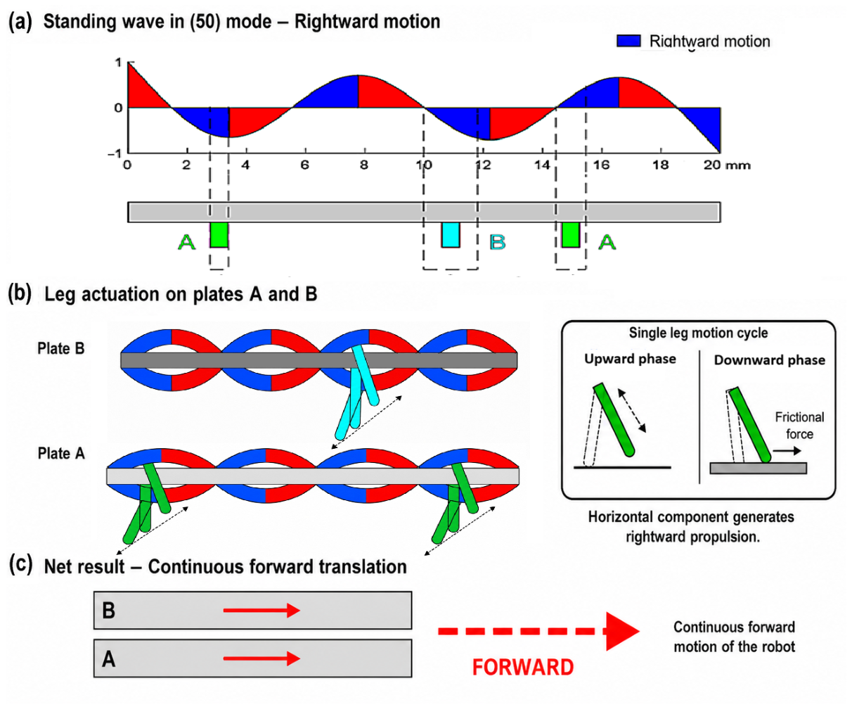
Figure 5.
Electronic schematics of the miniature robot.
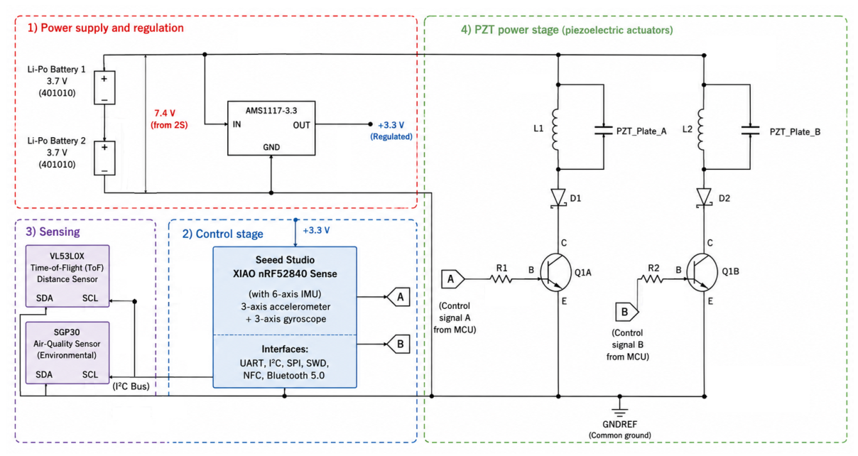
Figure 6.
Conductance versus frequency for piezoelectric plates A and B, showing the (50) and (60) modes.
Figure 6.
Conductance versus frequency for piezoelectric plates A and B, showing the (50) and (60) modes.
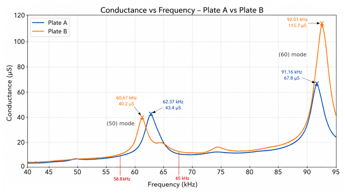
Figure 7.
Output voltage of the LC resonant tank in the power stage, measured for an input signal with a 50% duty cycle while varying the excitation frequency from 58 to 65 kHz.
Figure 7.
Output voltage of the LC resonant tank in the power stage, measured for an input signal with a 50% duty cycle while varying the excitation frequency from 58 to 65 kHz.
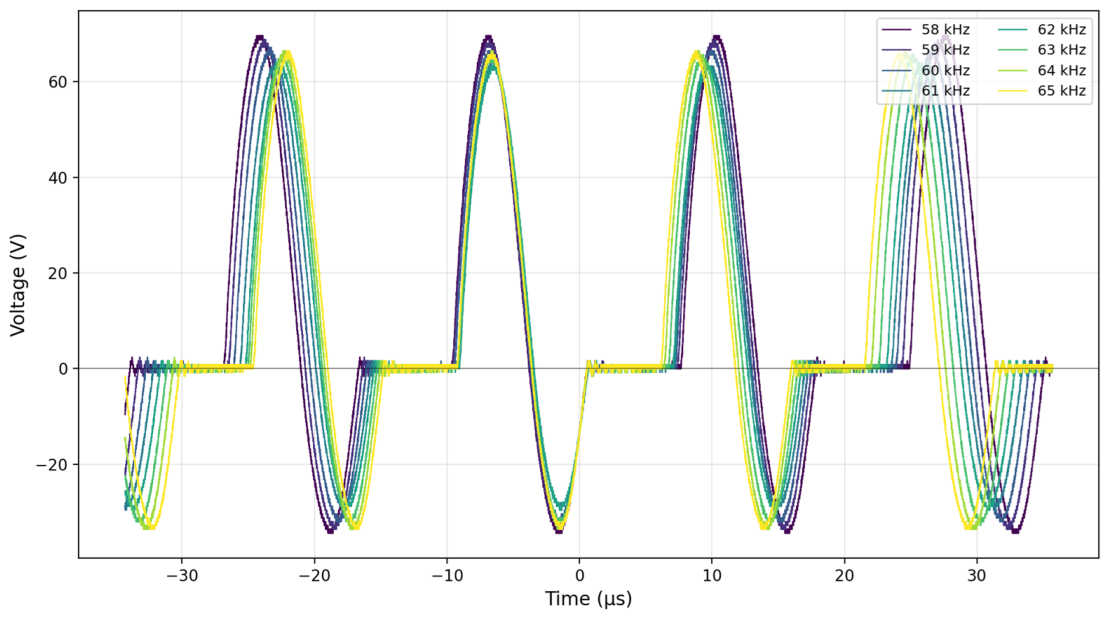
Figure 8.
Structural design of the robot frame: (a) three-dimensional view showing the arrangement of the main structural components; (b) overall dimensions used for fabrication and integration into the robot; and (c) three-dimensional view of the assembled structure with the integrated electronic components.
Figure 8.
Structural design of the robot frame: (a) three-dimensional view showing the arrangement of the main structural components; (b) overall dimensions used for fabrication and integration into the robot; and (c) three-dimensional view of the assembled structure with the integrated electronic components.
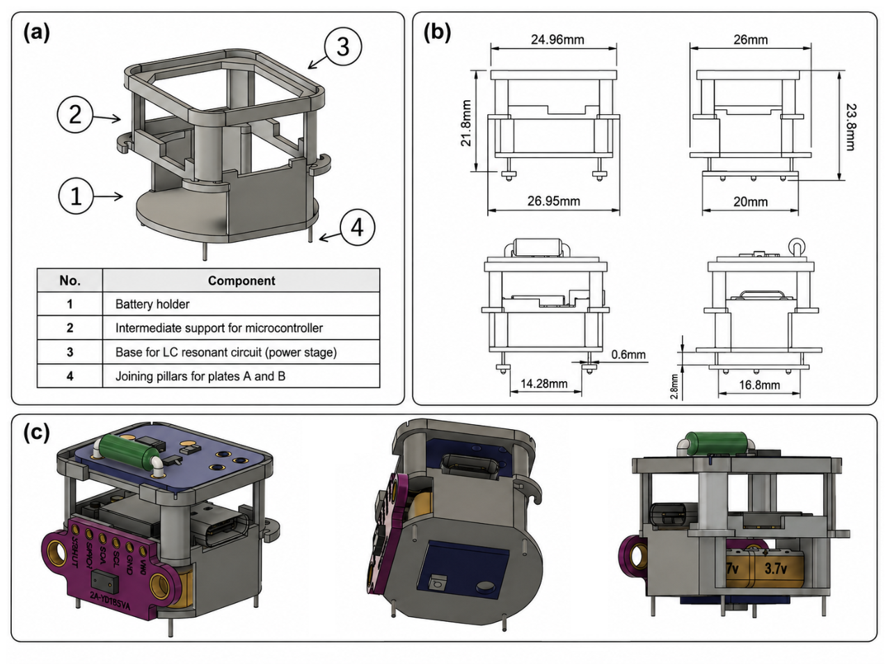
Figure 9.
Final implementation of the miniature robot with the onboard electronic and sensing components integrated into the 3D-printed structure: (a) front-side view and (b) bottom-side view.
Figure 9.
Final implementation of the miniature robot with the onboard electronic and sensing components integrated into the 3D-printed structure: (a) front-side view and (b) bottom-side view.
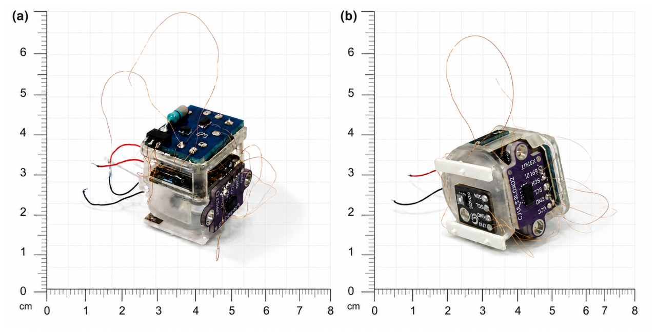
Figure 10.
Analysis of the pillar placement for mounting the robot structure: (a) deformation and displacement magnitude of Plate A at a frequency of 53.93 kHz; (b) deformation and displacement magnitude of Plate B at its eigenfrequency of 58.04 kHz; and (c) and (d) displacement profiles along the arc length for the Z-component.
Figure 10.
Analysis of the pillar placement for mounting the robot structure: (a) deformation and displacement magnitude of Plate A at a frequency of 53.93 kHz; (b) deformation and displacement magnitude of Plate B at its eigenfrequency of 58.04 kHz; and (c) and (d) displacement profiles along the arc length for the Z-component.
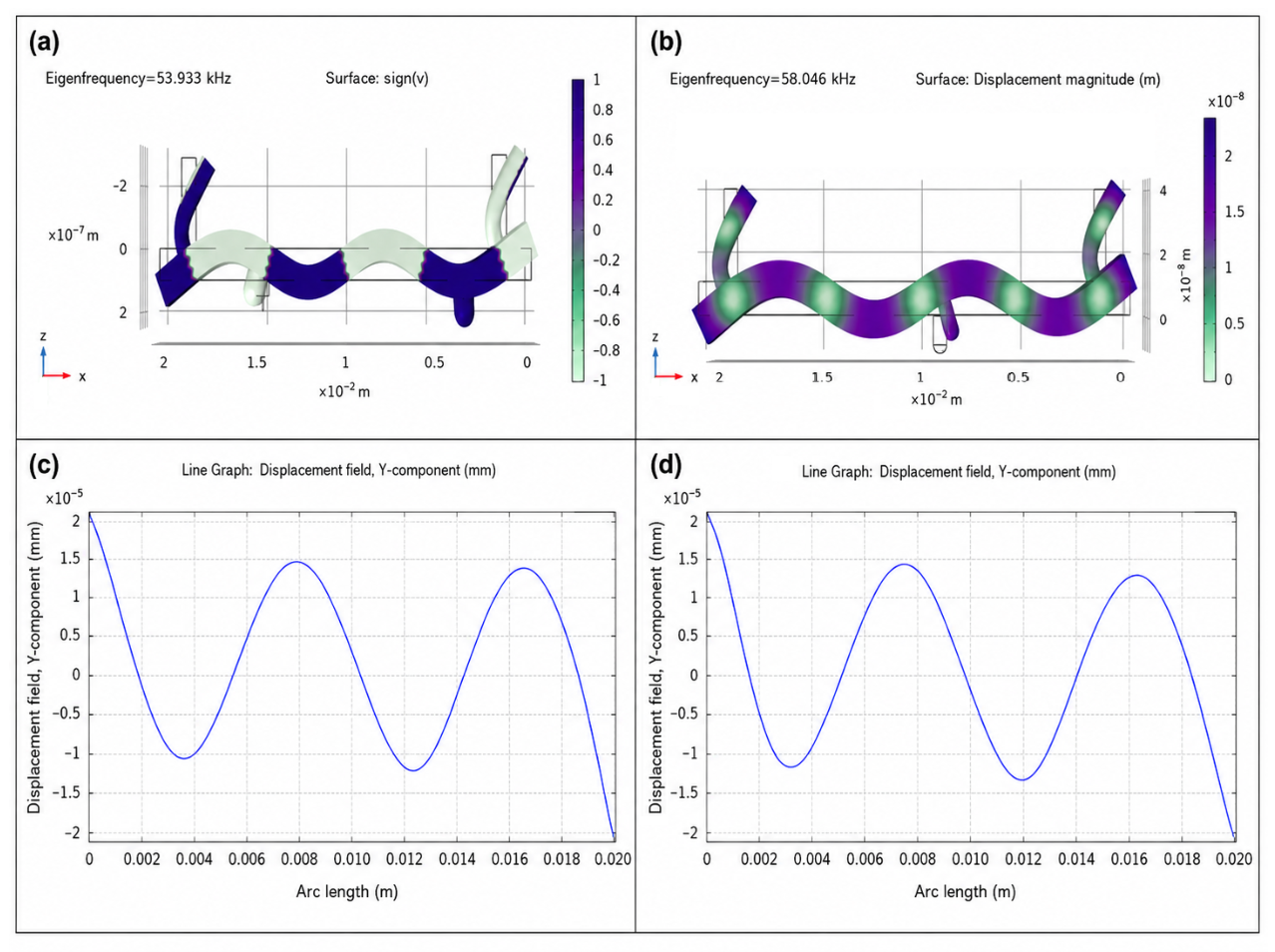
Figure 11.
Block diagram for the trajectory control of the miniature robot.
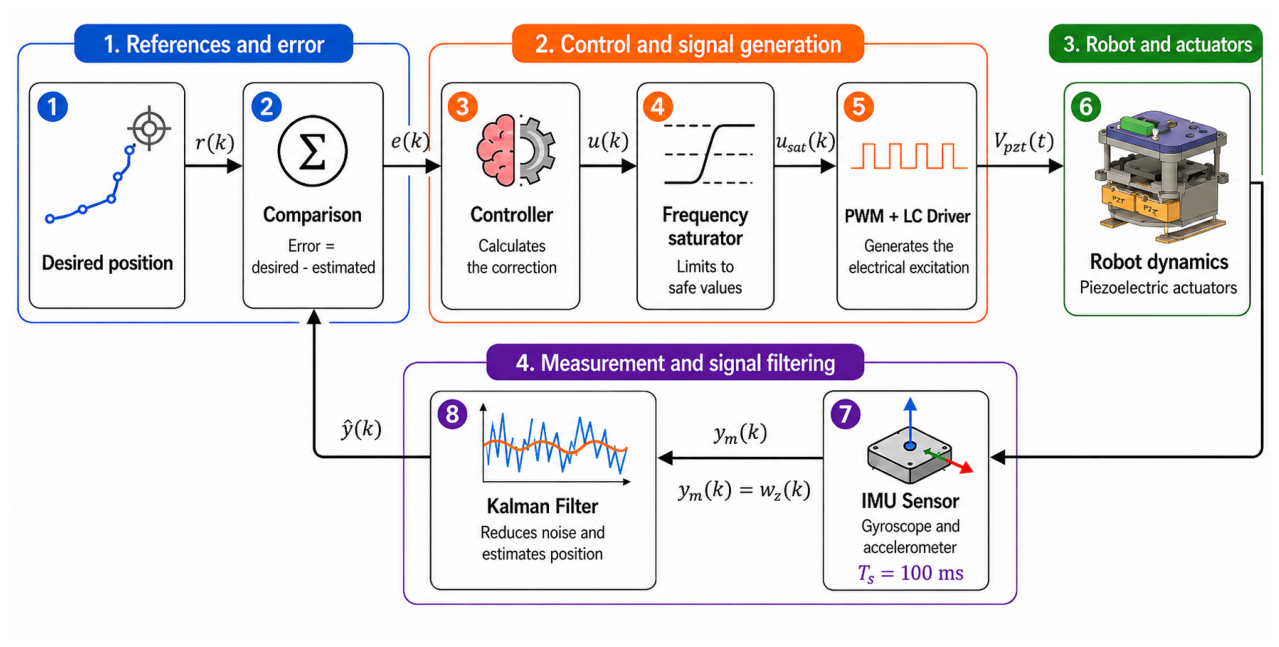
Figure 12.
Location of the VL53L0X and SGP30 sensors within the robot structure and their measurement characteristics for obstacle detection and TVOC monitoring, respectively.
Figure 12.
Location of the VL53L0X and SGP30 sensors within the robot structure and their measurement characteristics for obstacle detection and TVOC monitoring, respectively.
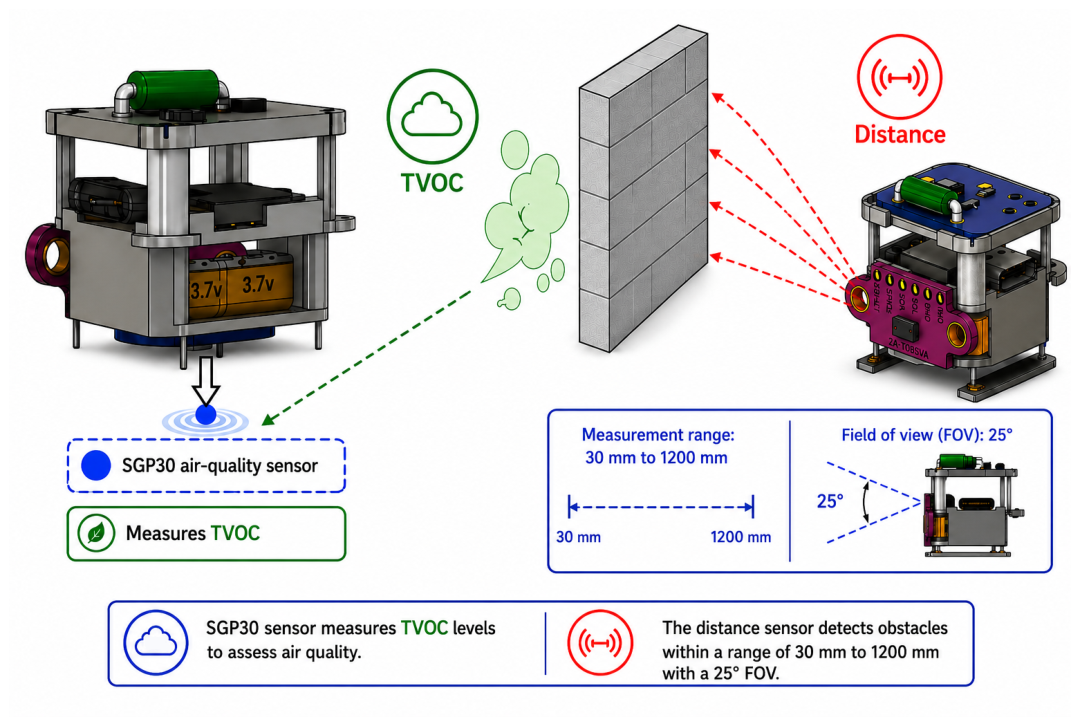
Figure 13.
Angular tracking response and control signals generated by the PD and SMC strategies for a constant 0°. The experiment can be observed in the Supplementary Video (Video S1).
Figure 13.
Angular tracking response and control signals generated by the PD and SMC strategies for a constant 0°. The experiment can be observed in the Supplementary Video (Video S1).
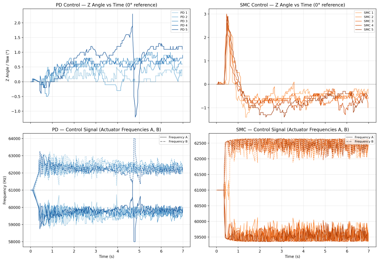
Figure 14.
Angular tracking response and control signals generated by the PD and SMC strategies with a reference change from 0° to 90°. The experiment can be observed in the Supplementary Video (Video S2).
Figure 14.
Angular tracking response and control signals generated by the PD and SMC strategies with a reference change from 0° to 90°. The experiment can be observed in the Supplementary Video (Video S2).
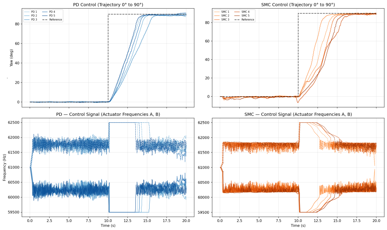
Figure 15.
Angular tracking response and control signals generated by the PD control with a reference change from 0° to 90° and return to 0°.
Figure 15.
Angular tracking response and control signals generated by the PD control with a reference change from 0° to 90° and return to 0°.
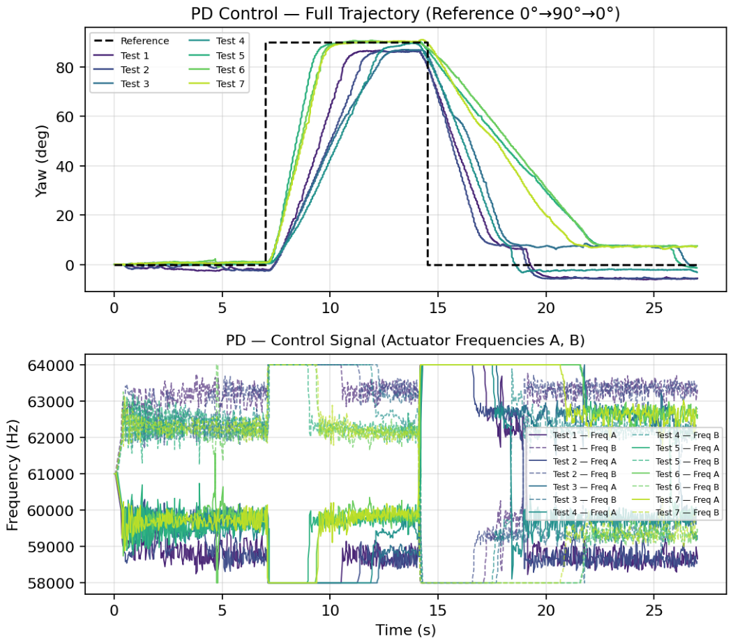
Figure 16.
Angular tracking response and control signals generated by the SMC control with a reference change from 0° to 90° and return to 0°.
Figure 16.
Angular tracking response and control signals generated by the SMC control with a reference change from 0° to 90° and return to 0°.
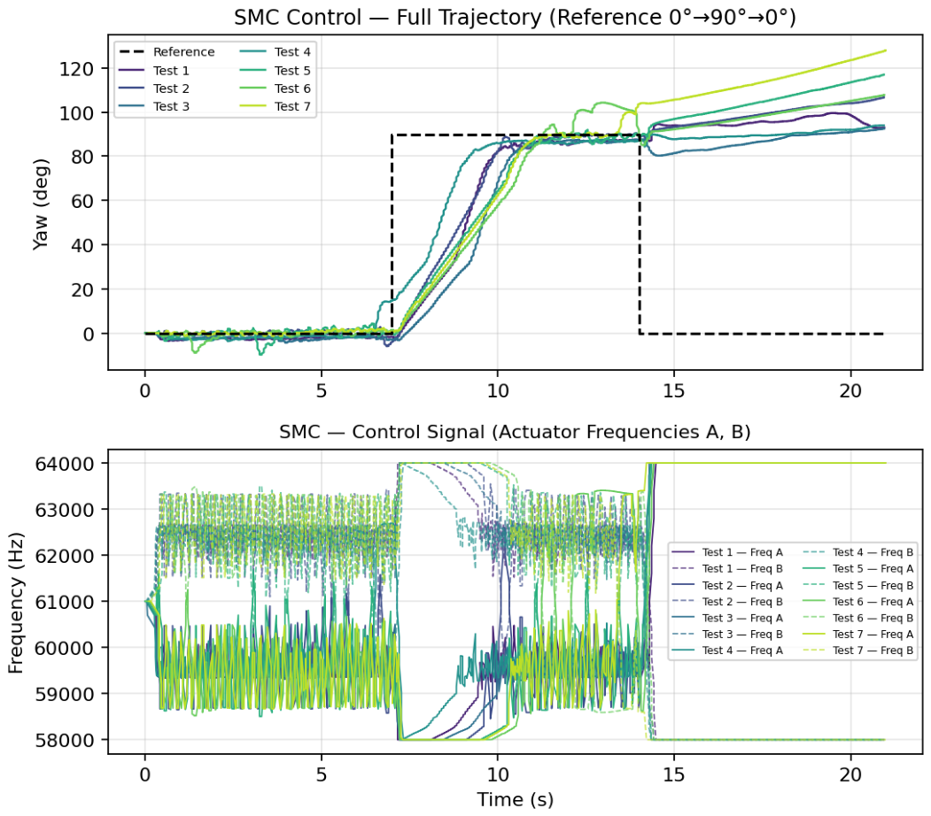
Figure 17.
Comparison of the robot’s linear and angular velocities using the PD and SMC controllers. Linear velocity is expressed in mm/s and body lengths per second (BL/s), whereas angular velocity is expressed in °/s.
Figure 17.
Comparison of the robot’s linear and angular velocities using the PD and SMC controllers. Linear velocity is expressed in mm/s and body lengths per second (BL/s), whereas angular velocity is expressed in °/s.
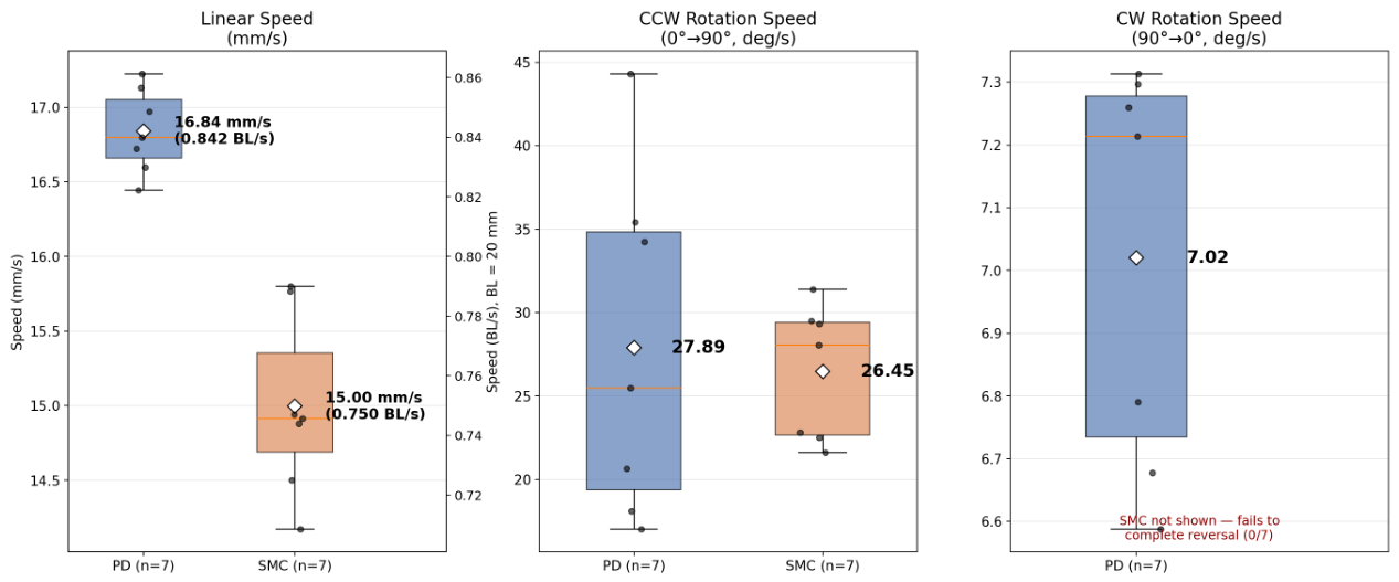
Figure 18.
Response of the PD and SMC controllers to a 0° reference after adding an additional weight of 9.35 g ( trials per controller). The experiment can be observed in the Supplementary Video (Video S3).
Figure 18.
Response of the PD and SMC controllers to a 0° reference after adding an additional weight of 9.35 g ( trials per controller). The experiment can be observed in the Supplementary Video (Video S3).
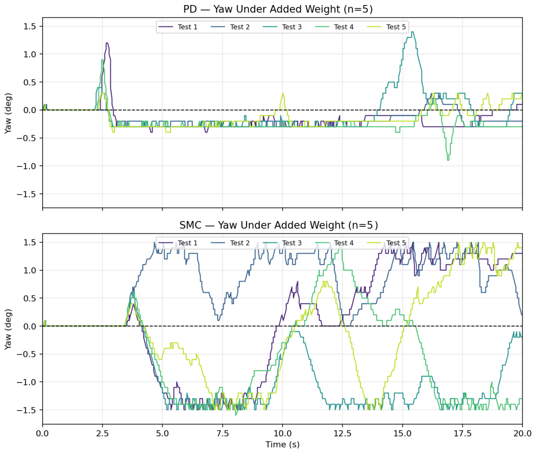
Figure 19.
Planned route for the environmental and spatial detection tests, showing the locations of the three measurement stations and the main dimensions of the circuit.
Figure 19.
Planned route for the environmental and spatial detection tests, showing the locations of the three measurement stations and the main dimensions of the circuit.
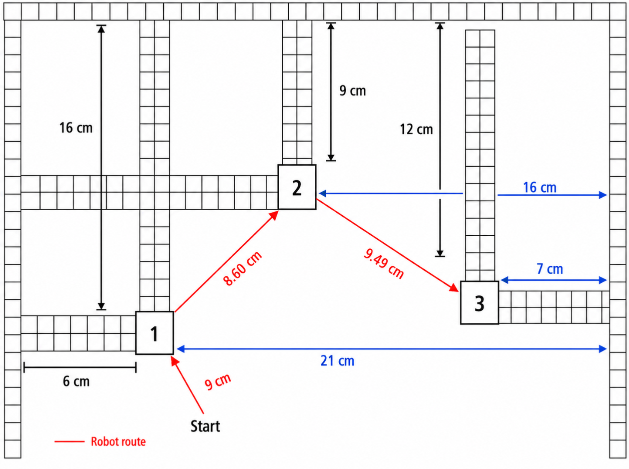
Figure 20.
Temporal response of and TVOC to exposure to of isopropyl alcohol at Station 2. The experiment can be observed in the Supplementary Video (Video S4).
Figure 20.
Temporal response of and TVOC to exposure to of isopropyl alcohol at Station 2. The experiment can be observed in the Supplementary Video (Video S4).
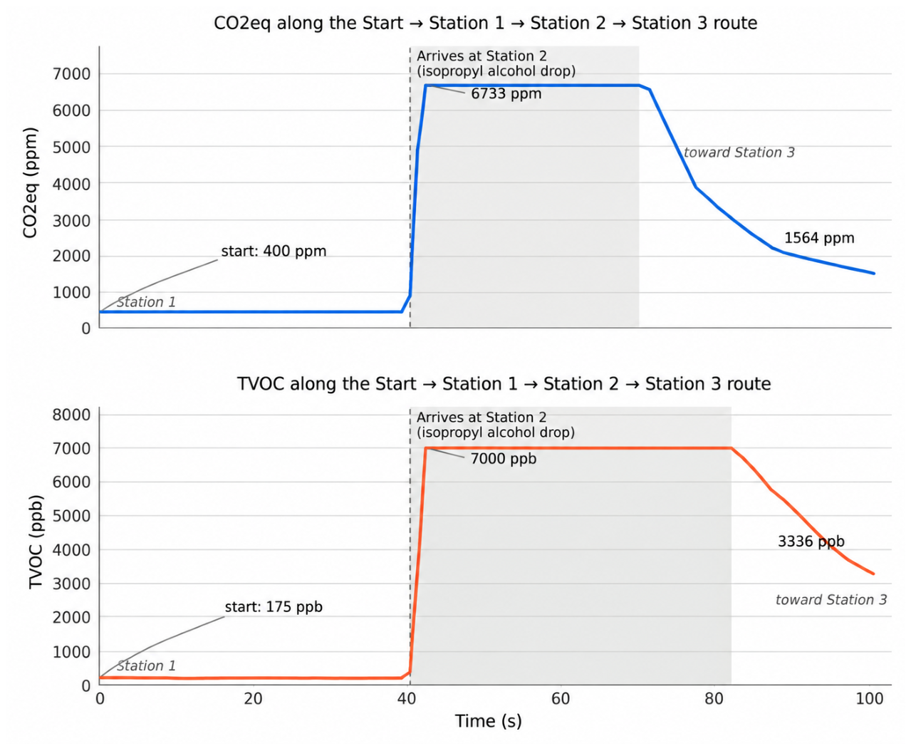

Table 1.
Design and manufacturing dimensions of Plates A and B.
| Symbol | Element and description | Dimension (mm) |
|---|---|---|
| L | Total plate length, measured between its two ends. | 20 |
| W | Plate width, corresponding to its transverse dimension. | 3 |
| H | Plate thickness, measured in the vertical direction. | 0.85 |
| Length of the PZT piezoelectric patch. | 5 | |
| Transverse width of the PZT piezoelectric patch. | 4 | |
| Longitudinal distance between Plates A and B. | 14.28 | |
| Leg height, measured from the lower surface of the plate to the end of the leg. | 1.1 | |
| Total height of Plate B, including its supporting leg. | 1.95 | |
| D | Leg diameter for Plates A and B. | 0.6 |
| Distance from the left end of Plate A to the center of the first leg. | 3 | |
| Distance from the center of the second leg to the right end of Plate A. | 5.7 | |
| Distance from the left end of Plate B to the center of its single leg. | 10.9 |
Table 2.
Peak-to-peak voltage () and root-mean-square current () measured at the output of the power stage for excitation frequencies ranging from 58 to .
Table 2.
Peak-to-peak voltage () and root-mean-square current () measured at the output of the power stage for excitation frequencies ranging from 58 to .
| f (kHz) | Vpp (V) | I (mA) |
|---|---|---|
| 58 | 104.0 | 25.0 |
| 59 | 102.4 | 24.7 |
| 60 | 99.2 | 24.6 |
| 61 | 93.6 | 24.6 |
| 62 | 93.6 | 24.7 |
| 63 | 98.4 | 24.6 |
| 64 | 100.0 | 24.2 |
| 65 | 100.0 | 23.7 |
Table 3.
Mass and dimensions of the robotic system’s constituent electronic components, including integrated sensors.
Table 3.
Mass and dimensions of the robotic system’s constituent electronic components, including integrated sensors.
| Elements | Quantity | Mass [g] | Dimension (L × W × H) [mm] |
|---|---|---|---|
| Microcontroller | 1 | 3.5 | 21 × 17.5 × 5 |
| Piezoelectric driver PCB | 1 | 2 | 22.2 × 18 × 10 |
| Batteries | 2 | 2.11 | 4 × 10 × 10 |
| VL53L0X sensor | 1 | 0.78 | 25 × 10 × 2 |
| SGP30 sensor | 1 | 0.46 | 19 × 19 × 3 |
| Magnetic programming pin | 1 | 0.96 | 10 × 5 × 10 |
| Total | 7 | 9.81 | – |
Table 4.
Angular performance metrics obtained for the PD and SMC controllers during the reference segment.
Table 4.
Angular performance metrics obtained for the PD and SMC controllers during the reference segment.
| Metric | PD Control | SMC Control |
|---|---|---|
| Mean absolute error (°) | 0.515 | 0.652 |
| Standard deviation (°) | 0.393 | 0.595 |
| Maximum peak (yaw) (°) | 2.300 | 3.000 |
Table 5.
Performance metrics obtained with the PD and SMC controllers in response to a reference change from 0° to 90° over five experimental trials per controller ().
Table 5.
Performance metrics obtained with the PD and SMC controllers in response to a reference change from 0° to 90° over five experimental trials per controller ().
| Metric | PD () | SMC () |
|---|---|---|
| Overshoot (%) | ||
| Rise time (s) | ||
| Settling time (s) | ||
| Final error (°) |
Table 6.
Performance metrics obtained with the PD control in response to a reference change from 0° to 90° and 90° to 0° over seven experimental trials ().
Table 6.
Performance metrics obtained with the PD control in response to a reference change from 0° to 90° and 90° to 0° over seven experimental trials ().
| Metric | PD — Up (), n=7 | PD — Down (), n=7 |
|---|---|---|
| Overshoot (%) | ||
| Rise/Fall time (s) | ||
| Settling time (s) | ||
| Final error (°) |
Table 7.
Angular performance metrics obtained for the PD and SMC controllers during posture correction with a 0° reference and additional weight.
Table 7.
Angular performance metrics obtained for the PD and SMC controllers during posture correction with a 0° reference and additional weight.
| Metric | PD Control | SMC Control |
|---|---|---|
| Mean absolute error (°) | 0.247 | 0.922 |
| Standard deviation (°) | 0.215 | 0.824 |
| Maximum peak (yaw) (°) | 0.840 | 1.520 |
Table 8.
Comparison between the reference distances and the mean distances measured by the VL53L0X sensor from five repeated measurements (n = 5) at the three stations along the trajectory.
Table 8.
Comparison between the reference distances and the mean distances measured by the VL53L0X sensor from five repeated measurements (n = 5) at the three stations along the trajectory.
| Position | True Coordinates () (cm) |
Mean Coordinates Measured by the Robot () () (cm) |
SD () (mm) |
CV () (%) |
Error () (cm) |
Mean Error (cm) |
|---|---|---|---|---|---|---|
| 1 | 0.96 | |||||
| 2 | 0.76 | |||||
| 3 | 0.97 |
Table 9.
Comparison of SGP30 TVOC readings against reference values and absolute percentage error across the three experimental stations.
Table 9.
Comparison of SGP30 TVOC readings against reference values and absolute percentage error across the three experimental stations.
| Station | Condition | SGP30 TVOC (ppb) |
Reference TVOC (ppb) |
Absolute Error (%) |
|---|---|---|---|---|
| 1 | Pre-source (baseline) | 175 | 201 | 12.94 |
| 2 | At alcohol source (peak) | 7000 | 7610 | 8.02 |
| 3 | Post-source (decreasing) | 3336 | 3168 | 5.30 |
Table 10.
Extended comparison between the miniature robot developed in this work and other miniature robots reported in the literature, including the presence of onboard IMU, distance, and gas sensors.
Table 10.
Extended comparison between the miniature robot developed in this work and other miniature robots reported in the literature, including the presence of onboard IMU, distance, and gas sensors.
| Microrobot Description | Size (mm) |
Total Mass (g) |
Speed (mm/s) |
Power Consumption (mW) |
Autonomy (min) |
Trajectory Control |
IMU | Distance Sensor |
Gas Sensor |
|---|---|---|---|---|---|---|---|---|---|
| This work | 26 | 12 | 16.84 | 360 | ∼ 20 (m) | Yes | Yes | Yes | Yes |
| Zapata Chancusig & Heredia Velastegui[23] | 26 | 9 | 8.87 | 444 | 24 (m) | Yes | Yes | No | No |
| Bimorphs and 3D-Printed Legs [8] | 17 | 7.42 | 70 | 50.5 | 406 (e) | No | N/R | N/R | N/R |
| BHMot [22] | 20 | 1.76 | 350 | 1770 | 3 (m) | No | No | No | No |
| HARM-F [20] | 45 | 2.8 | 172 | 600 | 4.5 (m) | No | N/R | N/R | N/R |
| DEAnsect [33] | 40 | 1 | 12 | 188 | 14 (e) | No | N/R | N/R | N/R |
| S2worm [34] | 41 | 4.34 | 30 | 610.5 | 13 (e) | No | N/R | N/R | N/R |
| PVDF robot [24] | 24 | 1.9 | 28.8 | 397 | 19 (e) | No | N/R | N/R | N/R |
| Legged piezoelectric resonator robot [15] | 27 | 7 | 15 | N/R | N/R | No | No | No | No |
| MilliMobile [35] | 10 | 1.1 | 5.5 | 0.05 | N/R | No | No | No | No |
| Tripodal piezoelectric microrobot [36] | 12.2 | 30 | 612 | ∼49 (m) | Yes | Yes | Yes (position) | Yes |
Disclaimer/Publisher’s Note: The statements, opinions and data contained in all publications are solely those of the individual author(s) and contributor(s) and not of MDPI and/or the editor(s). MDPI and/or the editor(s) disclaim responsibility for any injury to people or property resulting from any ideas, methods, instructions or products referred to in the content. |
© 2026 by the authors. Licensee MDPI, Basel, Switzerland. This article is an open access article distributed under the terms and conditions of the Creative Commons Attribution (CC BY) license (http://creativecommons.org/licenses/by/4.0/).
Copyright: This open access article is published under a Creative Commons CC BY 4.0 license, which permit the free download, distribution, and reuse, provided that the author and preprint are cited in any reuse.