

Submitted:
21 September 2026
Posted:
22 September 2026
You are already at the latest version
Abstract
Rapid-transit stations are usually judged as transport nodes, yet the walkable area around them decides whether residents can meet daily needs nearby. This study treats each station area as a service system and measures the supply of five civic dimensions (sports, commerce, health, green space and schools) within the 15-min walking catchments of the 125 operating stations of the Santiago Metro, Chile. Catchments were routed on a directed, slope-sensitive pedestrian network, and census counts were allocated by cadastral residential floor area. A Civic Deficit Index, defined against the network benchmark, was checked against census active-commuting shares, and an output-oriented data envelopment analysis frontier was estimated with bootstrap bias correction. One standard deviation of deficit was associated with a 2.65-percentage-point lower active-commuting share after controls. Seventeen station areas (13.6%) formed the frontier; mean efficiency was 0.623 (0.525 after bias correction) and mean scale efficiency 0.891. The two measures agreed partially (ρ = 0.446), and four station areas fell in the worst decile of both. Rankings were stable to weights, typology, frontier specification, peer removal, walking threshold and elevation error, whereas agreement with an order-m partial frontier was moderate (ρ ≈ 0.40). A priority matrix links station area to land-use instruments.
Keywords:
transit-oriented development
; station area
; civic infrastructure
; 15-minute city
; data envelopment analysis
; walking catchment
; backup coverage
; decision support
; land-use planning
; Santiago de Chile
1. Introduction
Transit-oriented development (TOD) [1] rests on the evidence that density, diversity and design around stations shape travel behaviour [2,3], and it is now a standard strategy against car dependence and dispersed growth [4]; the interaction between rail transit and land use remains an active and growing line of research [5]. The node–place model [6] and its extensions [7] read a station both as a node of the transport network and as a place of urban activity. Recent work adds a support dimension to that model [8] and links station performance to the land use and facilities around stations [9,10]. In most applications, however, the place side is still measured as the intensity and mix of activities. Whether the walkable area around a station contains the facilities residents use every day (a school, a health post, a park, a sports ground, local shops) has received less attention in station-area assessments.
The ‘15-minute city’ moved the discussion from mobility to proximity [11,12], reviving older neighbourhood-planning ideas [13]. Reviews report fast uptake and many operational definitions [14,15], and critics warn against using the idea as a ready-made brand detached from local conditions [16]. Empirical studies measure proximity with cumulative-opportunity or coverage indicators and time or distance thresholds [17,18,19,20]. They often find unequal walking access to amenities [21,22,23], including in Santiago, where proximity varies with socio-economic segregation [24], and they link proximity to health care and transit with higher life satisfaction [25]. Two lessons from this work matter for station areas. Accessibility is a joint property of land use and the transport network [26,27], so a catchment drawn as a Euclidean buffer misstates the territory reachable on foot [28], more so on sloping ground, where walking-speed assumptions change which areas fall inside a threshold [29,30]. And most proximity indicators are composite scores normalised against a threshold or a sample statistic. Such a score says how far a place is from a reference value, not whether that value is attainable given its population and land, which is what a land-use or investment decision needs.
Operations research and transport engineering offer tools for both problems, although operations research has had limited uptake in urban planning [31]. Location science defines the coverage of a facility as the demand within a maximum travel time [32], and it separates demand covered once from demand covered by a second facility, because single coverage fails when that facility is unavailable [33]. Transport-network analysis frames the same concern as vulnerability: losing a node matters most for the users who have no alternative route to the network [34]. Productivity analysis compares performance with the best observed practice instead of an average. Data envelopment analysis (DEA) estimates the frontier spanned by the best-performing units without assuming a functional form [35,36]. It has a long record in the evaluation of public services [37], including municipal infrastructure and equipment [38] and, more recently, park provision [39] and territorial space use with geographically defined peer groups [40]. Studies of public-facility layout, for their part, compare walkable supply with demand to locate shortfalls [41,42]. A frontier estimated from a finite sample lies inside the true one, so its scores are biased and need bootstrap correction before units are compared [43]. Seen through these tools, a station area is a service system: a routed catchment with a resident demand, whose output is the civic supply that demand can reach on foot.
The empirical case is the Metro of Santiago, Chile, with 125 operating stations on seven lines serving a conurbation of more than six million residents. Metro investment is capitalised into land and housing prices [44,45], and high-rise development concentrates near major transit in pericentral areas [46]. The public-space contributions required from intensive residential projects fall short of municipal investment plans [47]; green space is concentrated in high-income municipalities [48], and the diversity and structure of its tree cover also vary with income [49]; access to transit and to good walking environments is unequal [50]; and municipal zoning ordinances differ widely in their social provisions [51]. Santiago’s commuter-rail stations hold unexploited TOD potential [52], and national instruments could act at station scale: National Urban Development Policy (PNDU) [53], the System of Urban Development Indicators and Standards (SIEDU) [54] and a law on contributions to public space [55]. The most widely used synthetic index, the Urban Quality of Life Index (ICVU) [56], works at municipal scale, which is too coarse for station areas: a single central municipality can contain more than a dozen stations.
This study asks two questions. Does the walkable area around each operating station contain the civic infrastructure expected of a complete neighbourhood? And how far is each station area from what comparable station areas already achieve? The physical supply of five civic dimensions (sports and recreation, local commerce, health establishments, green space and schools) is measured inside 15-min catchments routed on a directed, slope-sensitive pedestrian network, and it is evaluated with two measures that share no mathematics: Civic Deficit Index (CDI) and an output-oriented DEA frontier with bootstrap bias correction. The paper makes four contributions. It offers a reproducible, parcel-based measurement of civic completeness at station scale for a whole metro network, built from the property cadastre, the 2024 Census and national registers and run as an automated pipeline that can be refreshed with each release of those registers. It relates the index to behaviour with a fractional-response model of active commuting. Its frontier analysis separates technical from scale shortfalls, states targets in physical units and checks, before estimating it, whether a second-stage regression can be identified. Finally, a priority matrix links deficit to land-use instruments, and thirteen robustness checks show which results depend on analyst choices. Section 2 presents data and methods, Section 3 the results, Section 4 the discussion and Section 5 the conclusions.
2. Materials and Methods
2.1. Research Design and Study Area
The workflow has two stages (Figure 1). The measurement stage builds the spatial framework, the pedestrian network, the catchments, the population layer and the civic inventory. The analytical stage estimates, on one fixed sample, the socio-urban typology, the deficit index and its validation, the efficiency frontier, the priority matrix and the robustness checks. The pipeline was built as a decision-support tool. A single notebook runs it end to end, declares every parameter and logs every exclusion and fallback with its count, so the assessment can be repeated and audited with each semi-annual cadastral release. That is the monitoring logic of urban digital twins [57], whose value for planning depends on how they are embedded in practice [58].
The study area is Greater Santiago, the continuous urban area formed by 34 municipalities, which contains the whole Metro network (2270 km²). Its boundary is the union of the 34 municipal polygons of the 2024 census cartography [59], and it was applied as a geometric filter to every geocoded source, because the municipal codes of the cadastre do not follow the census codes. Inside it, the census counted 6,171,091 residents in 56,453 blocks. The station registry lists 179 stations: 125 in operation on seven lines and 54 planned on Lines 7, 8 and 9 and the airport line, with which the network would reach 11 lines (Figure 2). Interchange stations are recorded once. Planned stations enter only the access contrast of Section 3.1.
The unit of analysis is the station area: the territory within a 15-min walk of an operating station, partitioned so that each hexagon belongs to the station it reaches fastest (Section 2.3). The threshold follows the proximity literature [11]; 12 and 18 min are tested as a robustness check, and 30 and 45 min are reported only as context.
2.2. Data and Spatial Framework
All sources are administrative or cartographic registers that cover the whole study area (Table 1). The property cadastre of the Internal Revenue Service (SII) [60] was read as 16 semi-annual snapshots (2018–2025) of property rolls and construction lines. Only the latest snapshot enters the results; the earlier fifteen were read to check the point-in-time consistency of the register and to leave the panel ready for later work. The analytical reference date is the second half of 2025 for the built stock, with the 2024 Census as the population base; the 2026 geocoding is used only to place parcels on the grid and carries no attribute of its own. A construction line records the floor area, land use and year of construction of each building on a parcel, so the register works as a ledger of the built stock; no price or transaction variable is used. All layers were aggregated to the H3 hexagonal grid [61] at resolution 9 (mean cell area 0.1053 km²), in line with the use of hexagonal cells in recent walking-access studies [18,62]. Parcels were mapped to cells once, before any aggregation: 3,279,846 parcels were geocoded individually, and 49,447 blocks served as a fallback. Between 8.5% and 9.9% of the cadastral records of each snapshot could not be located and were excluded without imputation. The share of construction lines dated after their own snapshot was 0.00% (of 4,898,040 lines in the second half of 2025), so the latest snapshot carries the full depth of the stock. In that snapshot, residential use accounts for 55.3% of built floor area, commerce for 5.6% and sports and recreation for 0.29% (Table S1).
Schools come from the directory of the Ministry of Education (MINEDUC) [63] and health establishments from the register of the Department of Health Statistics and Information (DEIS) [64]. Cutting a national register down to one metropolitan area discards most of its rows, so a provenance audit compared the location each record declares with the outcome of the geographic filters (Table S2). The recovery rate (records retained over records declared inside the study area) was 76.6% for schools and 91.5% for health establishments, and nearly all losses were records without coordinates (865 schools and 84 health establishments). Keeping operating facilities only, 2550 schools and 884 health establishments entered the analysis. Green space comes from a layer of parks and squares (4400 geometries, 26 of them points without area; 29.3 km²). Official registers were used wherever one covers the whole metropolitan area; green space and the street network come from OpenStreetMap, whose amenity coverage thins out towards the periphery [65]. The three registers are mapped in Figure S1–S3.
2.3. Directed Pedestrian Network and Station Catchments
Walking times were computed on a pedestrian graph built from 205,107 street centrelines taken from OpenStreetMap with Overpass Turbo [66] and projected to Universal Transverse Mercator (UTM) zone 19S. The query returned every way of the study area, with no filter by type, so motorway segments remain in the graph and footpaths absent from the source are missing from it. All polyline vertices were snapped to a 5 m grid, well below the width of any street, and 2360 duplicate arcs were reduced to the fastest one. The graph has 901,847 nodes and 1,037,620 edges in 327 components; the largest component holds 98.1% of the nodes. Each node takes the elevation of the nearest point of the elevation layer (152,190 points; median distance 39 m). Walking speed follows Tobler’s hiking function [67], and each edge carries one travel time per direction:
where ℓab is the length of edge ab (m), sab = (zb − za)/ℓab is its slope from a to b, v is in km/h and times are in minutes. Speed peaks at 6 km/h on a gentle descent (s = −0.05) and is about 5.04 km/h on level ground. The function is asymmetric, so climbing an edge takes longer than descending it; the relative difference between the two times is zero at the median (most edges are flat) and 18.8% at the 90th percentile. Keeping both times removes any dependence on the direction in which a segment was digitised, and the graph was routed as a directed network with 2,075,240 arcs.
Residents walk from home to the station. Travel times were therefore obtained with Dijkstra’s algorithm [68] run from each station on the reversed graph, which returns the time from every node to that station, up to a 50-min search limit. Each hexagon was represented by the location of one of its geocoded parcels, and hexagons and stations were snapped to the nearest node within 300 m (9527 of 9851 hexagons). Hexagons with no network route within 50 min (out of range, unsnapped or in a disconnected component) received a flagged straight-line estimate (great-circle distance at level-ground speed with a detour factor of 1.3). This fallback concerns hexagon beyond the routing horizon: at 15 min, 99.6% of the 4458 hexagon–station pairs came from network routing. Access was computed for the operating network and for the network extended with planned stations.
The served territory was then partitioned. Each hexagon within 15 min of at least one station was assigned to the station it reaches fastest, with ties broken by station identifier, which gives a walking-network Voronoi tessellation truncated at 15 min. In location-science terms, each station is a service node and its catchment is a service area bounded by a travel-time standard [32], with each unit of demand assigned to its closest node. It covers 2361 hexagons (248.7 km²); a catchment holds a median of 19 hexagons (10th–90th percentile: 9–29), and extents range from 0.42 to 3.79 km² (median 2.00 km²). Under a partition, network totals are additive and the frontier is estimated on units that do not share territory. The partition is an analytical convention rather than a boundary of use: residents can walk to a facility that falls in a neighbouring catchment, which is why the overlapping version is carried through the robustness checks. An overlapping version, in which a hexagon belongs to every station it reaches (4458 pairs; 1.89 stations per hexagon on average), was kept for sensitivity analysis. Central stations lie closer together, so their catchments are smaller (Spearman’s ρ = 0.565 between extent and distance to the historic centre); extent therefore enters the frontier as an input.
2.4. Population Allocation and Civic Dimensions
The census publishes counts by block, a unit unrelated to the grid. Counts were allocated to hexagons by dasymetric mapping [69,70,71], with residential floor area from the cadastre as the ancillary variable:
where popm is the count in block m, Sm,h is the residential (use H) floor area of the parcels of block m located in hexagon h, Ap is the residential floor area of parcel p and Sm that of the whole block. Of the residential parcels, 99.2% matched a block. The 14,232 blocks without residential floor area (1.8% of the population) were assigned to the hexagon of their centroid, so the allocated total equals the census total. The same weights were applied to every census count used later, and every rate is a ratio of sums within the catchment. Socio-economic vulnerability was measured with a block index (IST-2024) that averages four standardised shares: illiteracy, unrecoverable dwellings, overcrowding and unemployment. The index was built for this study from the census tables; it covers 42,783 blocks, and block values were averaged to hexagons and then aggregated to station areas with population weights, with higher values meaning greater disadvantage.
The construct is the physical supply of neighbourhood civic infrastructure inside the catchment, measured on five dimensions (Table 2). Units follow the object: sports grounds and green space are surfaces, because their size is the service, while shops, health establishments and schools are counted, because each serves a neighbourhood as a unit and counting premises prevents one shopping centre from standing in for many local shops. Each dimension has an absolute form, used as a DEA output, and a per-capita form, used in the CDI. A zero is a measurement, not a missing value, and all five dimensions were observed in all 125 station areas.
The sources limit what the dimensions mean in three ways. The health register does not identify the level of care, so all operating establishments are included. The cadastral dimension’s record declared land use in a tax register: use D (sports and recreation) appears in only 936 of 8194 built hexagons, and municipal grounds on public land may carry another use or none, so a zero on that dimension describes the cadastral record and does not prove that no facility exists. Green-space polygons were split across the hexagons they cover with a 40 m sampling lattice (3582 polygons); 792 polygons too small for the lattice went to their centroid cell, and the 26 point features add no area. Beyond these points, the dimensions do not measure quality, capacity, opening hours or use. Early-childhood care and frequency-weighted surface transit could not be measured, because the education directory used here does not separate levels of instruction and no General Transit Feed Specification (GTFS) feed was available, and neither was replaced by a proxy.
2.5. Network Form and Access Redundancy
Two context variables were measured on the graph; neither enters the CDI or the frontier. With the street network read as a primal graph [72], network form was described by intersection density, street density and mean node degree. Access redundancy follows the idea of backup coverage [33] and, in network terms, of node criticality [34]. For hexagon h, n15(h) is the number of stations reachable within 15 min, and for station area s
where C(s) is the partitioned catchment and 𝟙{·} is the indicator function. L(s) is the share of residents with no second station within 15 min: if the station closes, they have no other Metro station within walking reach, although other modes remain available.
2.6. Socio-Urban Typology
Station areas were grouped into socio-urban typologies (SUT) by k-means [73] on six standardised census variables: apartment share, housing-deficit rate, overcrowding rate, rental share, share aged 60 and over, and share aged 6–17. No spatial variable enters the clustering, so any geographic pattern in the deficit is a result, not an input. The algorithm ran with 30 initialisations and a fixed seed for k = 2, …, 8, and k was chosen with the Davies–Bouldin index [74] and the average silhouette [75]. Clusters were labelled from their centroids by a rule fixed in advance: SUT-M has the lowest apartment share (low-rise fabric); of the two apartment-dominated clusters, SUT-V has the higher housing deficit (vulnerable vertical fabric) and SUT-A is the other (consolidated apartment fabric). All 125 operating station areas had complete records, so none was excluded and nothing was imputed. The separation between groups is moderate (Section 3.2), so the typologies are analytical groupings, not natural urban types.
2.7. Civic Deficit Index and Behavioural Association
For station area s and dimension d, with per-capita provision yd(s) and benchmark bd, the index is
with weights wd. The lower truncation means that a surplus on one dimension cannot offset a shortage on another; a dimension with no supply scores 1, the maximum, so the upper truncation never binds. The index is left-censored by construction, so all correlations involving it are rank correlations. Two benchmarks were used:
where is the set of station areas and t(s) the typology of s. CDI-G compares every station area with the network median and tells whether it is under-provided relative to the network as a whole; CDI-S compares it with the median of its own typology. Both are relative measures: they locate provision below an observed benchmark and do not state compliance with a normative standard such as the SIEDU distances [54], which a station-level assessment could adopt instead (Section 4.3). A peer benchmark can hide absolute shortage, because a typology that is poorly served as a whole is only compared with itself. Statements about how provision is distributed across social groups therefore rest on CDI-G. Equal weights (wd = 1/5) are reported because nothing in the data ranks one civic dimension above another; entropy weights, first-principal-component weights and the mean DEA multiplier weights were used as alternatives.
The census records the main mode used by employed residents to travel to work. The share who walk or cycle enters neither index. It was related to CDI-G and CDI-S with Spearman’s ρ, and then to CDI-G with a fractional-response model [76], the aggregate counterpart of a random-utility choice model [77,78]:
where ys is the active-commuting share of station area s, Λ is the logistic function and xs contains the standardised CDI-G, IST-2024, log residential density, distance to the historic centre (Plaza de Armas) and dummies for SUT-M and SUT-V (reference: SUT-A). The model was fitted by Bernoulli quasi-maximum likelihood, weighted by the number of commuters, with heteroskedasticity-consistent (HC0) standard errors. The effect of interest is the average marginal effect (AME)
in percentage points of active-commuting share per standard deviation of deficit. The model describes a cross-sectional association and does not identify a causal effect.
2.8. Efficiency Frontier, Bias Correction and Second-Stage Identifiability
A median says how a station area compares with a typical one, not what supply is attainable for its population and land. DEA treats each station area as a decision-making unit that converts these endowments into civic supply. For unit o, with inputs xo and outputs yo, the output-oriented model with variable returns to scale (VRS) [36] is
with φ*o ≥ 1 and technical efficiency θo = 1/φ*o. Output orientation matches the planning question of how much more supply a station area could hold. Without the convexity constraint the model has constant returns (CRS) [35], and θCRS/θVRS is scale efficiency [36]. The model has m = 2 inputs (catchment population and walkable extent, km²) and q = 5 outputs in absolute units (sports floor area, commercial premises, health establishments, green area and schools). Extent is an input because a larger reachable area admits more facilities; outputs are absolute because ratio variables are incompatible with the standard constant-returns technology [79]. With n = 125, the rules n ≥ max{mq, 3(m + q)} = 21 [80] and n ≥ 2mq = 20 [81] are met. The 29 zero output cells (9 in sports, 18 in health and one each in green space and education) were kept as zeros; a radial expansion cannot lift a zero, so those gaps appear as slacks. Targets come from a second-phase programme that maximises slacks given φ*o, which yields φ*oyro + sr+ for each dimension r in its own unit. Frontier units were ranked by super-efficiency [82], and multiplier weights were taken from the dual. All programmes were solved with HiGHS in SciPy.
Bias-corrected scores and 95% intervals were obtained with the homogeneous smoothed bootstrap of Simar and Wilson [43] with B = 1000 replications. Pseudo-efficiencies were drawn from the estimated scores reflected about one and smoothed with a Gaussian kernel of bandwidth h = 1.06 min(σ̂, IQR/1.349) n−1/5 = 0.294 [83], then rescaled by (1 + h²/σ̂²)−1/2 so that the pseudo-sample keeps the variance of φ̂. Each replication contracts the observed outputs by φ̂/φ* to build a pseudo-technology and evaluates every unit against it (125,000 programmes). The bias and the corrected score are
with θbc = 1/φ̂̂o; the 95% interval for φ is φ̂ minus the 97.5th and 2.5th percentiles of φ* − φ̂, truncated at one, and inverting it gives the interval for θ. The correction is advisable when the squared bias exceeds one-third of the bootstrap variance, which was checked for each unit.
Whether distance to the frontier depends on context is usually examined with the truncated regression of Simar and Wilson [84],
where zi holds contextual covariates. Whether this design can identify such a regression was checked first by Monte Carlo simulation. The observed covariates (IST-2024, log density, distance to the centre and two typology dummies) and their collinearity were kept, the error scale was set to the observed standard deviation of φ̂, and a true IST-2024 effect of δ ∈ {0.10, 0.25, 0.50} standard deviations was imposed. The truncated estimator was refitted 200 times at each n ∈ {125, 250, 500, 1000, 2000}. The decision rule, fixed beforehand, was to estimate the second stage only if power reached 0.80 for a moderate effect at n = 125.
2.9. Structural Opportunity and Priority Matrix
A station area can lack provision where private investment is plausible or where it is not, and each case calls for a different instrument. Following the node–place logic [6,7], station areas were placed on two axes. The structural opportunity index (IO) is the mean percentile of walkable extent and of the normalised Shannon entropy [85] of built floor area across land-use classes,
where qk(s) is the floor-area share of class k and K the number of classes. The non-residential share of floor area was left out because it measures the same property (ρ = 0.952). The two axes share no variable, and their association was measured before quadrants were drawn. The composite priority index (IPI) is
where CDIGpct is the percentile of CDI-G, so a high score requires both opportunity and deficit. Quadrants split each axis at its network median: Q1, high opportunity and high deficit (TOD with civic priority); Q2, high opportunity and low deficit (market-led densification); Q3, low opportunity and high deficit (targeted public investment); and Q4, low opportunity and low deficit (consolidated provision). The matrix is a planning heuristic and not an estimate of what private investment will build: catchment size and land-use mix say nothing about land prices, unused development rights, vacant or underused sites, or the capacity of the municipality, and the quadrant labels should be read with that in mind. The matrix was also recomputed with the bias-corrected frontier deficit on the vertical axis. Agreement between the CDI and the frontier was measured with Spearman’s ρ, Kendall’s τ and the overlap of their worst deciles.
2.10. Robustness Checks and Reproducibility
Thirteen checks examined decisions already taken. (i) Spatial structure: global Moran’s I [86] of CDI-G with six nearest neighbours and 999 permutations, and local indicators of spatial association [87] with 199 permutations. (ii) Weighting scheme: the three alternative weight vectors. (iii) Weight uncertainty: 500 Dirichlet draws around equal weights (concentration scale 0.15), recomputing the index, the priority index and the quadrants. (iv) Number of typologies: k = 2 and k = 4, recomputing CDI-S and refitting the choice model with k − 1 dummies. (v) Frontier specification: overlapping catchments, per-capita outputs (with catchment extent as the only input), constant returns and bias-corrected scores. (vi) Extreme units: an output-oriented order-m partial frontier [88,89] with m = 25 and 50 and 500 Monte Carlo draws per unit, and a leave-one-out run that removes the three most frequent DEA peers, one at a time and together. (vii) Elevation error: node elevations were perturbed with a spatially correlated Gaussian field (σ = 2 m; squared-exponential covariance with a 100 m range, generated with 256 random Fourier features [90]) in 25 draws; each draw recomputed both directional times of every edge, rerouted all stations and rebuilt the partition. A first draw with σ = 0 served as control, and stability is reported against it. The field is correlated because neighbouring nodes share interpolation error; independent noise at both ends of a short edge would create false slopes. (viii) Walking threshold: catchments were rebuilt at 12 and 18 min and every measure recomputed, with the 15-min case rerun through the same code as a reproduction check. Five further checks address the measurement chain itself. (ix) Dimension left out: the index and the frontier were recomputed five times, each without one civic dimension. (x) Geography of the missing records: the share of register rows declared in a municipality without a usable coordinate was computed for schools and health establishments, keyed to the municipal code, and ranked against the deficit of the station areas of that municipality. (xi) Representative point: the network was rerouted from the geometric centre of every hexagon instead of a geocoded parcel, and the partition rebuilt. (xii) Residual spatial dependence: Moran’s I of the Pearson residuals of the choice model, with the weights of check (i). (xiii) Mode split: the choice model refitted on walking alone and on cycling alone.
The pipeline was written in Python with Python 3.12.13, pandas 2.3.3, NumPy 2.0.2, GeoPandas 1.1.3, Shapely 2.1.2, DuckDB 1.3.2, PyArrow 24.0.0, NetworkX 3.6.1, SciPy 1.16.3, scikit-learn 1.6.1, statsmodels 0.14.6, Matplotlib 3.10.0 and h3 4.5.0. A manifest records inputs, parameters, library versions and figures. Station-level results and frontier targets are provided in Table S3 and Table S4. Generative artificial intelligence (Claude, Anthropic) was used only to improve the wording of the manuscript; the data preparation, the analysis, the code and the interpretation of the results are the author’s own.
3. Results
3.1. Walking Access, Catchments and Redundancy
With the operating network, 24.0% of the geocoded hexagons of Greater Santiago lie within a 15-min walk of a station (Table 3; Figure 3). Coverage is higher when measured on population, because density is higher near the lines: 42.3% of residents live within 15 min of an operating station, 70.9% within 30 min and 85.0% within 45 min. The planned stations would raise 15-min coverage to 53.6% (Figure S4), a gain of 11.3 percentage points. At every threshold, at least 99.2% of hexagon–station pairs came from network routing (Figure S5 and Figure S6).
The 125 partitioned catchments hold 2,609,950 residents, and access redundancy is uneven (Figure 4). Of these residents, 1,017,689 (39.0%) can reach only one station within 15 min; if that station closed, they would have no other Metro station within a 15-min walk, although other modes would remain available. The mean of R(s) across station areas is 0.647 (median 0.686). On average, 2.3 stations are reachable within 15 min and the second one is 11.1 min away. The least redundant catchments are Lo Valledor (L(s) = 1.000), Cerrillos (0.996) and La Granja (0.932), all outside the central area where lines converge. Intersection density averages 330 per km² (range 144–665) and mean node degree 2.475, a low value because the graph keeps the shape vertices of each street, which have degree two.
3.2. Civic Provision and Socio-Urban Typologies
Four of the five dimensions are strongly right-skewed (Table 4), with coefficients of variation between 1.470 (health) and 1.926 (sports and recreation); education is more evenly spread (0.628). Zeros concentrate in two dimensions: 18 station areas have no health establishment, and 9 record no cadastral sports floor area, among them Pedro de Valdivia, a consolidated station area in Providencia, which illustrates the limitation noted in Section 2.4. The first principal component of the five standardised dimensions explains 39.5% of their variance, so a station area that is well served on one dimension is not necessarily well served on the others.
Both validity indices select k = 3 (Davies–Bouldin 0.854; silhouette 0.411; Table S5); the silhouette indicates moderate separation, so the groups are working categories rather than sharply distinct urban types. The typologies differ mostly in housing (Table S6). SUT-M, the largest group (56 station areas), has the lowest apartment and rental shares and the oldest population; SUT-A (45) is the most vertical and the least strained; and SUT-V (24) combines a high apartment share with the highest housing deficit, overcrowding and rental share. Against the network median, SUT-M falls below one on four dimensions (0.81–0.88). SUT-V has 1.71 times the network median of local commerce but the least green space (0.63), and SUT-A is at or above the median on all five dimensions, most clearly in health (1.82).
3.3. Civic Deficit Index and Behavioural Association
CDI-G has a mean of 0.242 (standard deviation 0.167), a median of 0.222 and a maximum of 0.673; CDI-S has a mean of 0.240 and a maximum of 0.722. Half of the station–dimension cells are zero under both benchmarks, and the untruncated gap reaches −37.63, so letting surpluses offset shortages elsewhere would mask deficits. The two benchmarks rank the network almost identically (ρ = 0.962; τ = 0.842; eight of the ten worst in common), but they point to different typologies (Figure 5). SUT-M has the highest mean CDI-G (0.276, against 0.218 in SUT-A and 0.211 in SUT-V), whereas SUT-A has the highest mean CDI-S (0.253). SUT-V, with the worst housing conditions, has the lowest mean CDI-G. Measured against the network benchmark, then, the civic shortfall lies in the low-rise, ageing fabric and not in the typology with the greatest housing strain.
Table 5 lists the ten highest CDI-G values. Laguna Sur (0.673), Vicuña Mackenna (0.636) and San Alberto Hurtado (0.603) head the list; four of the ten are on Line 5, and six fall in Q3 of the priority matrix.
The index moves with behaviour recorded independently of it. Across the network, a higher CDI-G goes with a lower share of commuters who walk or cycle (ρ = −0.491; p < 0.001), and the same holds within SUT-A (−0.565; p < 0.001), SUT-M (−0.354; p = 0.007) and SUT-V (−0.417; p = 0.042); CDI-S gives similar values (−0.477 for the network; Table S7). The fractional-response model confirms the association under controls (Table 6). The coefficient of the standardised CDI-G is −0.228 (robust SE 0.024; p < 0.001), an average marginal effect of −2.65 percentage points per standard deviation of deficit. Distance to the centre is the only other significant covariate (−0.88 points per km); vulnerability, density and typology are not significant in this model. The deviance pseudo-R² is 0.616, and observed and fitted shares correlate at 0.787. The association holds for walking on its own (−2.24 points per standard deviation; mean share 10.4%) and is weaker for cycling (−0.41 points; 3.8%), as a pedestrian catchment would predict (Table S17). The Pearson residuals are spatially clustered (Moran’s I = 0.374; pseudo p = 0.001), so the robust standard errors understate the uncertainty of the coefficient: the sign and size of the association are informative, its p-value is optimistic.
3.4. Efficiency Frontier
Seventeen station areas (13.6%) lie on the VRS frontier. Mean technical efficiency is 0.623 under VRS and 0.552 under CRS, and mean scale efficiency is 0.891; nine station areas have a scale efficiency of one. Most of the inefficiency is therefore technical. The frontier set mixes central SUT-A station areas on Line 1 (Universidad de Chile, Los Héroes, La Moneda) with peripheral SUT-M ones such as Plaza de Puente Alto (20.4 km away), Plaza de Maipú and Lo Valledor, and with SUT-V ones such as Parque O’Higgins. Super-efficiency, computable for 14 of the 17 frontier units, is highest for Universidad de Chile (4.19), Los Héroes (3.10) and Parque O’Higgins (2.56).
Bias correction lowers mean efficiency from 0.623 to 0.525. The mean interval width is 0.138, the correction criterion holds for all 125 units and no interval of an originally efficient unit reaches one, so frontier membership becomes a statement about intervals. The least efficient station areas stand clearly apart (Figure 6; Table S8). Rodrigo de Araya (θbc = 0.102) and Carlos Valdovinos (0.111) would need several times their current supply, and seven of the ten least efficient units are SUT-M.
The decomposition isolates a separate group (Figure 7). Eleven station areas have θ ≥ 0.90 but scale efficiency below 0.90, among them Bío Bío, El Bosque, Lo Valledor, Manquehue and Plaza de Maipú (Table S3). Their supply matches that of comparable units, but their catchments are either thinly populated, as in Lo Valledor (2823 residents; scale efficiency 0.571), or large, as in Manquehue (3.48 km²; 0.551). What they lack is catchment size or form, not facilities.
The targets locate the gaps (Table 7). The median gap relative to observed supply is largest for sports and recreation (176%) and health (175%), followed by commerce (134%), green space (97%) and education (64%). In health and sports, 59.75% and 50.63% of the gap is slack, meaning that it is concentrated in particular station areas, whereas the education gap is almost entirely radial (1.06% slack). The largest single gaps concern cadastral sports floor area, as in Quilín (from 33 to 16,648 m²).

Table 7.
Distance of the network from its own frontier, by civic dimension.
| Dimension | Unit | Median relative gap ¹ | Median absolute gap | Network total | Share via slack |
| Sports and recreation | m² | 176% | 3209 | 534,763 | 50.63% |
| Health establishments | establishments | 175% | 6.1 | 730 | 59.75% |
| Local commerce | premises | 134% | 411 | 50,614 | 40.89% |
| Green space | m² | 97% | 36,322 | 6,939,827 | 16.74% |
| Education | schools | 64% | 6.6 | 830 | 1.06% |
Gaps are target minus observed supply; totals are additive because catchments partition the served territory. Share via slack: part of the gap not delivered by the radial expansion. ¹ Station–dimension cells with zero observed supply are excluded, because the relative gap is undefined for them. Targets are physical supply, not capacity or investment requirements (Figure 8; Table S4).
Figure 8.
Relative distance to the frontier target by civic dimension, one marker per station area.
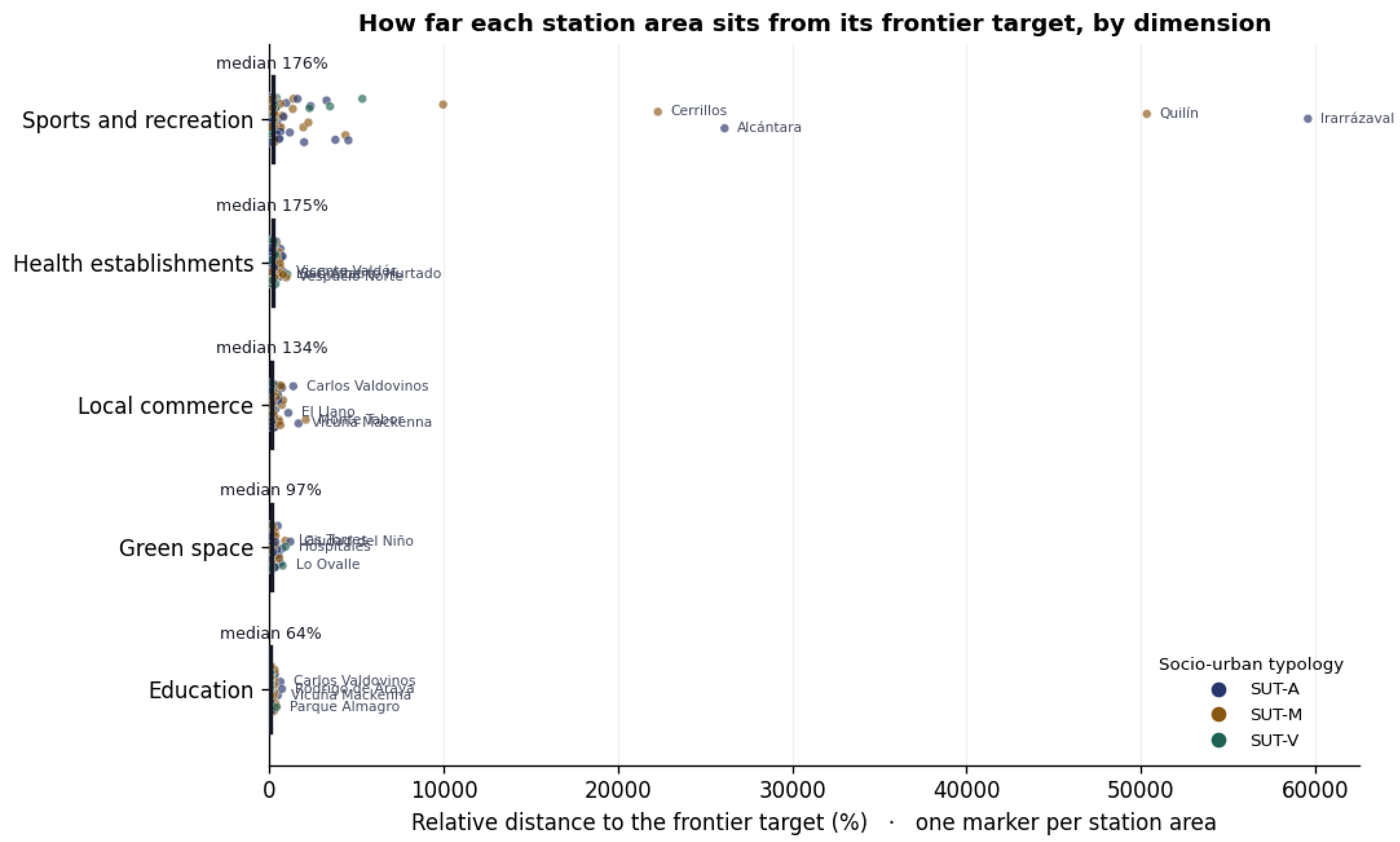
The two ends of the distribution differ on every dimension (Figure S13–S17): the 17 frontier units average 89.35 commercial premises per 1000 residents and 10.43 m² of green space per resident, against 7.95 and 2.49 in the 12 units of the lowest decile of θbc.
The power experiment rules out a second stage (Figure S18; Table S9). At n = 125, the probability of detecting a small, moderate or large effect (δ = 0.10, 0.25 and 0.50) is 10%, 24% and 78%. A power of 0.80 would require between 125 and 250 station areas for a large effect, between 500 and 1000 for a moderate one and more than 2000 for a small one. Following the rule fixed in advance, no second-stage coefficient was estimated.
3.5. Agreement Between the Two Measures
CDI-G and the bias-corrected frontier deficit agree partially (ρ = 0.446; τ = 0.305; p < 0.001); for CDI-S the value is 0.400. Agreement is similar within SUT-A (0.430) and SUT-M (0.423) and weak and not significant within SUT-V (0.110; p = 0.610). Four station areas lie in the worst decile (12 units) of both measures: Laguna Sur (CDI-G 0.673; θbc 0.240), Vicuña Mackenna (0.636; 0.152), Rodrigo de Araya (0.564; 0.102) and Del Sol (0.550; 0.200). Three are on Line 5 and one on Line 4, and Del Sol and Vicuña Mackenna record no cadastral sports floor area.
The largest disagreements follow two patterns. Station areas that the index ranks worse than the frontier either serve many residents, as Irarrázaval (41,803) does, so that the index spreads supply over many people while the frontier asks what is attainable for that many, or are scale-inefficient, as Lo Valledor is. In the other direction, El Golf and Los Dominicos have low per-capita deficits (CDI-G 0.071–0.140) but lie far from the frontier (θbc 0.298–0.369).
3.6. Structural Opportunity and Priority Matrix
Land-use entropy and the non-residential share are nearly interchangeable (ρ = 0.952), and the two-component IO agrees with a three-component version at ρ = 0.828. IO ranges from 17.8 in Lo Prado to 91.8 in Plaza de Puente Alto. Opportunity and deficit are moderately and negatively related (ρ = −0.349; p < 0.001): station areas with more mixed land use and larger catchments tend to be better served, which makes Q1 and Q4 the less frequent quadrants.
With the medians as cut-off points (IO 49.8; CDI-G percentile 50.4), Q2 holds 41 station areas, Q3 40, Q1 23 and Q4 21 (Figure 9; the quadrants are mapped in Figure S20). The highest priority indices belong to Rodrigo de Araya (82.1), Cerrillos (80.4) and Hospitales (77.2), all in Q1. Of the four station areas flagged by both measures, Rodrigo de Araya is in Q1, while Laguna Sur, Vicuña Mackenna and Del Sol are in Q3, where the conditions for private provision are weaker. With the bias-corrected frontier deficit on the vertical axis, 36.8% of station areas change quadrant; the horizontal axis is unchanged, so every move takes place within the same opportunity class.
3.7. Robustness
Table S10 summarises the checks. Deficit is spatially clustered (Moran’s I = 0.189; pseudo p = 0.001), with a high–high cluster of nine SUT-M station areas in the west of the city, six of them on Line 5. The ordering of the index is stable across weighting schemes and under weight uncertainty, and re-estimating the typology with two or four groups barely changes CDI-S or the marginal effect of CDI-G.
The frontier ordering holds across specifications (ρ from 0.746 to 0.979). The order-m frontiers agree less with DEA (ρ ≈ 0.40; six of the ten least efficient units in common), and 67–78% of units lie beyond the partial frontier, partly because order-m drops convexity. Plaza de Puente Alto, La Moneda and Parque O’Higgins serve as peers for 99, 50 and 47 of the 108 inefficient units, yet removing them, one at a time or together, keeps the ordering of the remaining units at ρ ≥ 0.982.
The partition is insensitive to the elevation interpolation. The σ = 0 control reproduced 99.9% of hexagon statuses and all station assignments, with coverage of 42.255% against the reported 42.341% because it does not repeat the straight-line fallback. Against the control, the 25 correlated draws kept the served status of 99.81% of the 9851 hexagons on average (at most 26 hexagons changed) and the assigned station of 99.56%; coverage fell by 0.11 points on average (standard deviation 0.06), and every draw stayed below the control (Figure S21). Five checks address the measurement chain (Table S18–S20). Leaving out one civic dimension at a time leaves the deficit ordering in place (ρ between 0.870, without sports, and 0.966, without commerce) and the frontier ordering too, except when education is removed (ρ = 0.708; mean θ falls from 0.623 to 0.393), so the education count carries more of the frontier than any other output. The registers lose coordinates where provision is best: within Greater Santiago, 865 of 3706 declared schools (23.3%) and 84 of 978 health establishments (8.6%) have no usable coordinate, with the highest rates in Macul (41.9%), Providencia (39.1%) and San Miguel (36.7%) and the lowest in La Pintana (9.5%), and the municipal loss rate does not rank with the deficit (ρ = −0.117; p = 0.193). Rerouting from the geometric centre of each hexagon instead of a geocoded parcel moves the representative point by a median of 151 m and keeps the served status of 97.3% of hexagons and the assigned station of 89.2% of those served under both, with population coverage 0.75 points lower: the interior of every catchment is stable and its boundary is not. The threshold matters more still. At 12 and 18 min, the served population moves from 2.61 million to 2.12 and 3.06 million, but ρ is 0.952 and 0.919 for CDI-G and 0.967 and 0.932 for the frontier, and 86.4% and 81.6% of station areas keep their quadrant.
4. Discussion
4.1. The Station Area as a Service System
Living near the Metro does not make a neighbourhood complete: 42.3% of Santiago’s residents live within a 15-min walk of a station, but station areas differ widely in what they contain. Proximity studies usually ask whether services can be reached from where people live [17,18,19,20], and supply–demand studies of public facilities report similar mismatches at neighbourhood scale [41,42]. Taking the station area as the unit moves the question to the scale at which TOD decisions are made [4,6,7], where municipal indices such as the ICVU [56] cannot see. In engineering terms, each station area is a service system with a demand (its residents), a service area (its routed catchment) and a capacity to serve (its civic stock). The frontier measures its productivity against peers, as a logistics planner would compare depots serving similar demand. Backup-coverage logic [33] adds a reliability reading: for 39.0% of catchment residents the station is a critical node with no alternative within walking reach, the situation that network-vulnerability studies describe [34].
The shortfall is not where housing indicators would place it. Against the network benchmark it is concentrated in the low-rise, ageing fabric of SUT-M and not in SUT-V, which has the worst housing conditions but is comparatively well served with shops and health establishments and poorly served with green space. The green-space gap of the vulnerable vertical fabric is consistent with the concentration of green areas in high-income municipalities [48] and with income-related differences in the diversity and structure of their tree cover [49]; transit-related inequities in park access have also been reported for Mexico City [91]. The broader deficit of SUT-M suggests that, in intermediate and peripheral neighbourhoods, Metro access has not been matched by civic equipment, while high-rise growth has favoured pericentral areas near transit [46], and the high–high cluster in the west, mostly along Line 5, indicates a corridor-scale problem. Together with the evidence on unequal access to transit and walking environments [50] and on proximity and segregation measured with fixed buffers [24], this shows that a station within reach does not guarantee what residents need around it.
The behavioural association gives the construct empirical content. One standard deviation of deficit is associated with a share of active commuting 2.65 points lower, with vulnerability, density, distance and typology held constant. The sign is the one the built-environment literature predicts for the local availability of destinations [2,3]. The outcome is the trip to work, whose destination usually lies outside the catchment, so the association may reflect neighbourhood qualities that go together with civic supply rather than trips to the facilities themselves. That density is not significant in a model that includes deficit and location is relevant for TOD practice, which gives density a central role [4].
4.2. What Each Measure Adds
Partial agreement (ρ = 0.446) is what two instruments aimed at the same construct from different directions should produce. The CDI states shortfall against a convention; the frontier states it against what comparable station areas already deliver, the logic that Prieto and Zofío applied to municipal equipment [38]. The frontier also tells what kind of shortfall it is. With mean scale efficiency at 0.891, most gaps are supply gaps that can be closed by locating facilities. For the eleven station areas that are efficient in supply but not in scale, the relevant levers are different: pedestrian permeability, station entrances, or the land-use rules that set the size and population of the catchment. The mix of central and peripheral units on the frontier shows that best practice is not tied to one social profile.
Three design choices shape how the results should be read. The bootstrap [43] removes the notion of an unambiguously efficient unit, so rankings are read as overlapping intervals. The power experiment shows that one network of 125 station areas cannot support a second-stage truncated regression of the Simar–Wilson type [84]; reporting that finding, instead of a coefficient that could not be interpreted, avoids a frequent problem in small DEA applications. The question can be taken up with pooled networks or with the semi-annual cadastral panel, or by bringing context into the frontier itself, through geographic peer groups [40] or non-controllable variables [92]; double-bootstrap studies of park provision show what a larger sample allows [39]. Finally, the ordering of station areas survives changes in weights, typology, frontier specification, peers and threshold, but convexity builds demanding virtual peers and may overstate technical inefficiency, and leaving out one dimension at a time shows that the frontier leans on the education count more than on any other output, so the targets are best read as orders of magnitude for planning, not as exact quotas.
4.3. Implications for Land-Use Policy
The matrix maps result onto instruments. In Q1 (23 station areas), mixed land use and large catchments coexist with high deficit, so densification can be conditioned on civic supply. The public-space contribution law [55], whose contribution regime has applied since November 2020 [93], and value capture in general [94] provide the mechanism, the capitalisation of Metro investment into land and housing prices [44,45] provides the fiscal base, and the frontier targets indicate which dimension each contribution should fund. The Shenzhen rail-plus-property model shows, however, that value capture rests on market and institutional conditions that are hard to transfer [95]. In Q2 (41), supply is adequate relative to the network, but contributions from dense projects fall short of municipal investment plans [47], so per-capita supply should be monitored as population grows. Q3 (40) combines weak conditions for private supply with high deficit; provision there is likely to require public investment, and three of the four station areas flagged by both measures belong to this group. Q4 (21) calls for maintenance rather than expansion.
At national level, SIEDU [54], developed under the PNDU [53], already sets proximity standards, such as a maximum distance of 400 m to a square, 1000 m to a basic-education school, 1500 m to a primary-care centre and 3000 m to a park [96]; a 15-min walk on level ground covers about 1.26 km. The PNDU update, approved by the Interministerial Committee for City, Housing and Territory (COMICIVYT) in December 2025 and sent for final legal processing [97], offers a chance to add a station-level version that applies these standards dimension by dimension where transit investment concentrates, and to planned stations before they open. The 11.3-point coverage gain expected from the planned lines makes that assessment timely, since Line 7 is under construction and expected to open at the end of 2028 [98]. Instruments, however, are not equally available everywhere. Greater Santiago is governed by 34 municipalities with very unequal revenue and planning capacity, and their zoning ordinances differ widely in what they require of projects [51], so a Q3 station area in a low-revenue peripheral municipality faces a different implementation problem from a Q1 station area in a pericentral one, even when the measured deficit is the same. Where a station area is both deficient and non-redundant, as in Lo Valledor and Cerrillos, residents cannot compensate by walking to another station. Planning transit, land use and social infrastructure together is the practical route towards the sustainable-city targets of the 2030 Agenda [99].
4.4. Transferability and Limitations
The method requires a property register, a census, facility registers and a street network with elevation, which most metropolitan areas hold in some form, and its node–place logic fits the extended station-area models now used elsewhere [8]. The parameters that would change between cities (threshold, snapping tolerance, dimensions) are explicit, and the robustness checks show which results depend on them. Several limitations remain. (i) The construct is physical supply; quality, capacity, opening hours and use are not measured, and targets are counts and surfaces. (ii) The cadastral sports dimension depends on declared land use and is under-recorded, which inflates its deficits and targets; half of its frontier gap is slack, so those targets should be read as a signal to check the ground and not as a requirement to be written into a contribution or a plan. (iii) Neither the health nor the education register is graded: a regional hospital counts like a local clinic and a large secondary school like a small primary one, so a station area that happens to contain a large facility can look better provided than daily life around it would suggest. (iv) Of the schools declared inside the study area, 865 (23.3%) lack coordinates; that loss is concentrated in well-provided municipalities and does not rank with the deficit (Section 3.7), but it remains a source of noise in the education dimension. (v) The outcome is the commute to work, the model is associational, and its residuals are spatially clustered, so the standard errors are a lower bound. (vi) With 125 units, estimates for SUT-V (n = 24) are imprecise. (vii) Part of the efficiency ranking depends on the convexity assumption of DEA. (viii) Elevations come from nearest-point interpolation (median distance 39 m); the correlated-error experiment bounds the effect of random error on the partition, but not a systematic bias of the elevation source. (ix) Hexagons are routed from one representative point, and the choice of that point moves about a tenth of the boundary assignments (Section 3.7).
Future work can add a GTFS-based surface-transit layer and a care dimension (early-childhood providers such as the Junta Nacional de Jardines Infantiles (JUNJI) and Fundación Integra, and services of the Servicio Nacional del Adulto Mayor (SENAMA) for older adults). Rerun after each semi-annual cadastral release, the pipeline would work as a station-area monitoring system in the spirit of urban digital twins [57]. The resulting panel would relate civic supply to densification around stations, and pooling station areas from several Latin American networks would provide the sample needed to explain distance to the frontier. A covering-location model [32] could then turn the targets into specific sites.
5. Conclusions
This study measured civic completeness in the 125 operating station areas of the Santiago Metro using directed, slope-sensitive walking catchments, parcel-based population estimates and administrative registers that cover the whole metropolitan area. A deficit index and a bias-corrected efficiency frontier agree partially and jointly single out Laguna Sur, Vicuña Mackenna, Rodrigo de Araya and Del Sol as the most deficient station areas. A higher deficit goes with less active commuting after controls, most inefficiency is technical rather than a matter of scale, and only 13.6% of station areas define best practice. The shortfall measured against the network benchmark is concentrated in low-rise, ageing station areas and in a contiguous cluster in the west of the city, and 39.0% of catchment residents depend on a single station. The rankings withstand the robustness checks, although part of the efficiency ranking rests on the convexity assumption of DEA.
For land-use policy, transit accessibility and neighbourhood completeness should be assessed together. The priority matrix distinguishes station areas where densification can be tied to civic provision through contributions and value capture from those where provision is likely to require public investment, and the frontier targets express, in physical units, each station area’s gap to a model-based benchmark. Because the method runs on registers that most cities keep and as an automated, logged pipeline, it can be applied before new stations open, repeated as the registers are updated and transferred to other metro networks.
Supplementary Materials
The following supporting information can be downloaded at the website of this paper posted on Preprints.org, Table S1: Land-use composition of the built stock; Table S2: Provenance audit of the facility registers; Table S3: Station-area table; Table S4: Frontier targets by station area and dimension; Table S5: Typology validity; Table S6: Socio-urban typologies; Table S7: Deficit and active commuting; Table S8: Ten least efficient station areas; Table S9: Second-stage power; Table S10: Summary of the robustness checks; Tables S11–S16: Sensitivity to weights, number of typologies, frontier specification, order-m frontier, peer removal and walking threshold; Table S17: The model refitted on each active mode; Table S18: The index and the frontier without one civic dimension; Table S19: Register rows without a usable coordinate; Table S20: Rerouting from the geometric centre of each hexagon; Figures S1–S3: Register maps; Figure S4: Walking access with the planned stations; Figures S5–S6: Access-time distribution and coverage curve; Figures S7–S11: Provision distributions; Figure S12: Choice-model fit; Figures S13–S17: Frontier units against the lowest decile; Figure S18: Power curve; Figure S19: Priority matrix with every station area named; Figure S20: Priority quadrants map; Figure S21: Elevation-error experiment.
Author Contributions
Conceptualization, methodology, software, validation, formal analysis, investigation, data curation, writing—original draft preparation, writing—review and editing, visualization, G.U. The author has read and agreed to the published version of the manuscript.
Funding
This research received no external funding. The article processing charge is funded by Universidad Finis Terrae.
Institutional Review Board Statement
Not applicable.
Informed Consent Statement
Not applicable.
Data Availability Statement
The source data are publicly available from the Servicio de Impuestos Internos (property cadastre), the Instituto Nacional de Estadísticas (2024 Census), the Ministerio de Educación (directory of educational establishments) and the Departamento de Estadísticas e Información de Salud (register of health establishments). The analysis notebook, the reproducibility manifest and the derived station-area tables are available from the author on reasonable request.
Acknowledgments
The author thanks the Vicerrectoría de Investigación, Creación Artística e Innovación of Universidad Finis Terrae for its support. During the preparation of this manuscript, the author used Claude (Anthropic) to improve the wording of the text. The author reviewed and edited the output and takes full responsibility for the content of this publication.
Conflicts of Interest
The author declares no conflicts of interest.
References
- Calthorpe, P. The Next American Metropolis: Ecology, Community, and the American Dream; Princeton Architectural Press: New York, NY, USA, 1993. [Google Scholar]
- Cervero, R.; Kockelman, K. Travel Demand and the 3Ds: Density, Diversity, and Design. Transp. Res. Part D. Transp. Environ. 1997, 2, 199–219. [Google Scholar] [CrossRef]
- Ewing, R.; Cervero, R. Travel and the Built Environment: A Meta-Analysis. J. Am. Plan. Assoc. 2010, 76, 265–294. [Google Scholar] [CrossRef]
- Ibraeva, A.; Correia, G.H.d.A.; Silva, C.; Antunes, A.P. Transit-Oriented Development: A Review of Research Achievements and Challenges. Transp. Res. Part A Policy Pract. 2020, 132, 110–130. [Google Scholar] [CrossRef]
- Yang, H.; Cui, N.; Xia, H. The Evolution of the Interaction Between Urban Rail Transit and Land Use: A CiteSpace-Based Knowledge Mapping Approach. Land 2025, 14, 1386. [Google Scholar] [CrossRef]
- Bertolini, L. Spatial Development Patterns and Public Transport: The Application of an Analytical Model in the Netherlands. Plan. Pract. Res. 1999, 14, 199–210. [Google Scholar] [CrossRef]
- Vale, D.S. Transit-Oriented Development, Integration of Land Use and Transport, and Pedestrian Accessibility: Combining Node-Place Model with Pedestrian Shed Ratio to Evaluate and Classify Station Areas in Lisbon. J. Transp. Geogr. 2015, 45, 70–80. [Google Scholar] [CrossRef]
- Li, J.; Shen, Z.; Ma, J.; Hao, Y.; Zeng, R.; Lin, Z. Evaluation of Sustainable Development Potential of Railway Station Areas in Guangzhou Metropolitan Area: Based on the Extended “Node–Place–Support” Model. Land 2025, 14, 369. [Google Scholar] [CrossRef]
- Chen, H.; Zhao, K.; Zhang, Z.; Zhang, H.; Lu, L. Methods for the Performance Evaluation and Design Optimization of Metro Transit-Oriented Development Sites Based on Urban Big Data. Land 2024, 13, 1233. [Google Scholar] [CrossRef]
- Gao, Y.; Cui, X.; Sun, X. Land Use Characteristics of Commuter Rail Station Areas and Their Impact on Station Ridership: A Case Study of Japan Railways in the Tokyo Metropolitan Area. Land 2024, 13, 2045. [Google Scholar] [CrossRef]
- Moreno, C.; Allam, Z.; Chabaud, D.; Gall, C.; Pratlong, F. Introducing the “15-Minute City”: Sustainability, Resilience and Place Identity in Future Post-Pandemic Cities. Smart Cities 2021, 4, 93–111. [Google Scholar] [CrossRef]
- Allam, Z.; Nieuwenhuijsen, M.; Chabaud, D.; Moreno, C. The 15-Minute City Offers a New Framework for Sustainability, Liveability, and Health. Lancet Planet. Health 2022, 6, e181–e183. [Google Scholar] [CrossRef] [PubMed]
- Khavarian-Garmsir, A.R.; Sharifi, A.; Hajian Hossein Abadi, M.; Moradi, Z. From Garden City to 15-Minute City: A Historical Perspective and Critical Assessment. Land 2023, 12, 512. [Google Scholar] [CrossRef]
- Khavarian-Garmsir, A.R.; Sharifi, A.; Sadeghi, A. The 15-Minute City: Urban Planning and Design Efforts toward Creating Sustainable Neighborhoods. Cities 2023, 132, 104101. [Google Scholar] [CrossRef]
- Papadopoulos, E.; Sdoukopoulos, A.; Politis, I. Measuring Compliance with the 15-Minute City Concept: State-of-the-Art, Major Components and Further Requirements. Sustain. Cities Soc. 2023, 99, 104875. [Google Scholar] [CrossRef]
- Bonfantini, G.B.; Galimberti, B.; Ventura, E. There Are No ‘Solutions’ in Urban Planning: Against the Idea of a Ready-Made Urbanism and the 15-Minute City’s Uncritical Branding. Land 2025, 14, 2090. [Google Scholar] [CrossRef]
- Logan, T.M.; Hobbs, M.H.; Conrow, L.C.; Reid, N.L.; Young, R.A.; Anderson, M.J. The x-Minute City: Measuring the 10, 15, 20-Minute City and an Evaluation of Its Use for Sustainable Urban Design. Cities 2022, 131, 103924. [Google Scholar] [CrossRef]
- Radics, M.; Christidis, P.; Alonso, B.; dell’Olio, L. The X-Minute City: Analysing Accessibility to Essential Daily Destinations by Active Mobility in Seville. Land 2024, 13, 1656. [Google Scholar] [CrossRef]
- Thornton, L.E.; Schroers, R.-D.; Lamb, K.E.; Daniel, M.; Ball, K.; Chaix, B.; Kestens, Y.; Best, K.; Oostenbach, L.; Coffee, N.T. Operationalising the 20-Minute Neighbourhood. Int. J. Behav. Nutr. Phys. Act. 2022, 19, 15. [Google Scholar] [CrossRef] [PubMed]
- Chiaradia, F.; Lelo, K.; Monni, S.; Tomassi, F. The 15-Minute City: An Attempt to Measure Proximity to Urban Services in Rome. Sustainability 2024, 16, 9432. [Google Scholar] [CrossRef]
- Talen, E. Who Can Walk? An Analysis of Public Amenity Access in America’s Ten Largest Cities. Environ. Plan. B Urban Anal. City Sci. 2023, 50, 1775–1789. [Google Scholar] [CrossRef]
- Calafiore, A.; Dunning, R.; Nurse, A.; Singleton, A. The 20-Minute City: An Equity Analysis of Liverpool City Region. Transp. Res. Part D. Transp. Environ. 2022, 102, 103111. [Google Scholar] [CrossRef]
- Willberg, E.; Fink, C.; Toivonen, T. The 15-Minute City for All? – Measuring Individual and Temporal Variations in Walking Accessibility. J. Transp. Geogr. 2023, 106, 103521. [Google Scholar] [CrossRef]
- Israel, F.; Otero, G.; Soza-Parra, J.; Broitman, D. 15-Minute City, Proximity, and Urban Segregation in Latin-American Cities: The Case of Santiago de Chile. Transp. Res. Part A Policy Pract. 2026, 204, 104789. [Google Scholar] [CrossRef]
- Yasin, H.; Mohíno, I.; Carpio-Pinedo, J. Exploring the Relationship Between 15 Minute Access and Life Satisfaction. Land 2025, 14, 2259. [Google Scholar] [CrossRef]
- Hansen, W.G. How Accessibility Shapes Land Use. J. Am. Inst. Plan. 1959, 25, 73–76. [Google Scholar] [CrossRef]
- Geurs, K.T.; van Wee, B. Accessibility Evaluation of Land-Use and Transport Strategies: Review and Research Directions. J. Transp. Geogr. 2004, 12, 127–140. [Google Scholar] [CrossRef]
- Gutiérrez, J.; García-Palomares, J.C. Distance-Measure Impacts on the Calculation of Transport Service Areas Using GIS. Environ. Plan. B Plan. Des. 2008, 35, 480–503. [Google Scholar] [CrossRef]
- Pais, F.; Sousa, N.; Monteiro, J.; Coutinho-Rodrigues, J.; Natividade-Jesus, E. Walking to Public Transport: Rethinking Catchment Areas Considering Topography and Surrogate Buffers. ISPRS Int. J. Geo-Inf. 2025, 14, 205. [Google Scholar] [CrossRef]
- Rahman, F.; Oliver, R.; Crawford, T.; Buehler, R.; Lee, J.; Kim, J. How Walking-Speed Assumptions Shape 15-Minute City (15-MC) Accessibility Scores: A Case Study of Roanoke, Virginia. Future Transp. 2026, 6, 145. [Google Scholar] [CrossRef]
- Fabusuyi, T.; Johnson, M.P. Enhancing the Quality and Social Impacts of Urban Planning through Community-Engaged Operations Research. Environ. Plan. B Urban Anal. City Sci. 2022, 49, 1167–1183. [Google Scholar] [CrossRef]
- Church, R.; ReVelle, C. The Maximal Covering Location Problem. Pap. Reg. Sci. Assoc. 1974, 32, 101–118. [Google Scholar] [CrossRef]
- Hogan, K.; ReVelle, C. Concepts and Applications of Backup Coverage. Manag. Sci. 1986, 32, 1434–1444. [Google Scholar] [CrossRef]
- Mattsson, L.-G.; Jenelius, E. Vulnerability and Resilience of Transport Systems – A Discussion of Recent Research. Transp. Res. Part A Policy Pract. 2015, 81, 16–34. [Google Scholar] [CrossRef]
- Charnes, A.; Cooper, W.W.; Rhodes, E. Measuring the Efficiency of Decision Making Units. Eur. J. Oper. Res. 1978, 2, 429–444. [Google Scholar] [CrossRef]
- Banker, R.D.; Charnes, A.; Cooper, W.W. Some Models for Estimating Technical and Scale Inefficiencies in Data Envelopment Analysis. Manag. Sci. 1984, 30, 1078–1092. [Google Scholar] [CrossRef]
- Emrouznejad, A.; Yang, G. A Survey and Analysis of the First 40 Years of Scholarly Literature in DEA: 1978–2016. Socio-Econ. Plan. Sci. 2018, 61, 4–8. [Google Scholar] [CrossRef]
- Prieto, A.M.; Zofío, J.L. Evaluating Effectiveness in Public Provision of Infrastructure and Equipment: The Case of Spanish Municipalities. J. Product. Anal. 2001, 15, 41–58. [Google Scholar] [CrossRef]
- Benito, B.; Conesa-Pérez, M.d.C.; Parra-Meroño, M.-C. Determinants of Inefficiency in the Provision of Public Parks and Gardens Services. Cities 2025, 163, 106031. [Google Scholar] [CrossRef]
- Zheng, M.; Ma, Y.; Zheng, X.; Wang, X.; Li, L.; Xu, F.; Zhang, X.; Gan, F.; Wang, J.; Zhu, Z. Evaluating Territorial Space Use Efficiency: A Geographic Data Envelopment Model Considering Geospatial Effects. Land 2025, 14, 635. [Google Scholar] [CrossRef]
- Chen, C. Discussion on the Optimization Method of Public Service Facility Layout from the Perspective of Spatial Equity: A Study Based on the Central City of Shanghai. Land 2023, 12, 1780. [Google Scholar] [CrossRef]
- Li, T.; Fang, X.; Zhu, J.; Peng, Q.; Zhao, W.; Fu, X. Horizontal and Vertical Spatial Equity Analysis Based on Accessibility to Living Service Amenities: A Case Study of Xi’an, China. Land 2024, 13, 1113. [Google Scholar] [CrossRef]
- Simar, L.; Wilson, P.W. Sensitivity Analysis of Efficiency Scores: How to Bootstrap in Nonparametric Frontier Models. Manag. Sci. 1998, 44, 49–61. [Google Scholar] [CrossRef]
- Agostini, C.A.; Palmucci, G.A. The Anticipated Capitalisation Effect of a New Metro Line on Housing Prices. Fisc. Stud. 2008, 29, 233–256. [Google Scholar] [CrossRef]
- López-Morales, E.; Sanhueza, C.; Herrera, N.; Espinoza, S.; Mosso, V. Land and Housing Price Increases due to Metro Effect: An Empirical Analysis of Santiago, Chile, 2008–2019. Land Use Policy 2023, 132, 106793. [Google Scholar] [CrossRef]
- Moreno-Alba, D.; Marmolejo-Duarte, C.; Vicuña del Río, M.; Aguirre-Núñez, C. Urban Verticalisation: Typologies of High-Rise Development in Santiago. Build. Cities 2026, 7, 254–272. [Google Scholar] [CrossRef]
- Vicuña, M.; Pumarino, N.; Urbina, A. Pago por Impactos en Proyectos de Densificación Residencial Intensiva del Área Metropolitana de Santiago: Análisis Crítico de los Aportes al Espacio Público en la Nueva Legislación Chilena. EURE 2020, 46, 47–71. [Google Scholar] [CrossRef]
- Reyes Päcke, S.; Figueroa Aldunce, I.M. Distribución, Superficie y Accesibilidad de las Áreas Verdes en Santiago de Chile. EURE 2010, 36, 89–110. [Google Scholar] [CrossRef]
- Guevara, B.R.; Uribe, S.V.; de la Maza, C.L.; Villaseñor, N.R. Socioeconomic Disparities in Urban Forest Diversity and Structure in Green Areas of Santiago de Chile. Plants 2024, 13, 1841. [Google Scholar] [CrossRef] [PubMed]
- Tiznado-Aitken, I.; Muñoz, J.C.; Hurtubia, R. The Role of Accessibility to Public Transport and Quality of Walking Environment on Urban Equity: The Case of Santiago de Chile. Transp. Res. Rec. 2018, 2672, 129–138. [Google Scholar] [CrossRef]
- Vergara-Perucich, J.F. AI-Driven Deconstruction of Urban Regulatory Frameworks: Unveiling Social Sustainability Gaps in Santiago’s Communal Zoning. Urban Sci. 2025, 9, 186. [Google Scholar] [CrossRef]
- Vecchio, G. Estaciones como Nodos y Lugares: El Potencial del Tren para el Desarrollo Urbano Orientado al Transporte en Santiago, Chile. Urbano 2021, 24, 84–95. [Google Scholar] [CrossRef]
- Ministerio de Vivienda y Urbanismo (MINVU). Política Nacional de Desarrollo Urbano; MINVU: Santiago, Chile, 2014. [Google Scholar]
- Ministerio de Vivienda y Urbanismo (MINVU); Instituto Nacional de Estadísticas (INE); Consejo Nacional de Desarrollo Territorial (CNDT). Sistema de Indicadores y Estándares de Desarrollo Urbano (SIEDU). Available online: https://www.ine.gob.cl/herramientas/portal-de-mapas/siedu (accessed on 16 September 2026).
- Ley N° 20.958. Establece un Sistema de Aportes al Espacio Público. Diario Oficial de la República de Chile. 15 October 2016. Available online: https://www.bcn.cl/leychile/navegar?idNorma=1095541 (accessed on 16 September 2026).
- Instituto de Estudios Urbanos y Territoriales UC; Cámara Chilena de la Construcción. Índice de Calidad de Vida Urbana ICVU 2025: Una Mirada Retrospectiva; Pontificia Universidad Católica de Chile: Santiago, Chile, 2026; Available online: https://estudiosurbanos.uc.cl/documento/icvu-2025-calidad-de-vida-urbana-decada/ (accessed on 16 September 2026).
- Batty, M. Digital Twins. Environ. Plan. B Urban Anal. City Sci. 2018, 45, 817–820. [Google Scholar] [CrossRef]
- Azadi, S.; Kasraian, D.; Nourian, P.; van Wesemael, P.J.V. What Have Urban Digital Twins Contributed to Urban Planning and Decision Making? From a Systematic Literature Review Toward a Socio-Technical Research and Development Agenda. Smart Cities 2025, 8, 32. [Google Scholar] [CrossRef]
- Instituto Nacional de Estadísticas (INE). Censo de Población y Vivienda 2024: Bases de Datos a Nivel de Manzana y Cartografía. 16 December 2025. Available online: https://censo2024.ine.gob.cl/ine-publica-bases-de-datos-a-nivel-de-manzana-y-cartografia-del-censo-de-poblacion-y-vivienda-2024/ (accessed on 16 September 2026).
- Servicio de Impuestos Internos (SII). Catastro de Bienes Raíces: Detalle de Líneas de Construcción y Roles (Series BRORGA2441NL y BRORGA2441N). Available online: https://www.sii.cl https://www.sii.cl/bbrr/descargas/estructura_detalle_catastral.pdf (accessed on 16 September 2026).
- Uber Technologies; Inc. H3: A Hexagonal Hierarchical Geospatial Indexing System. Available online: https://h3geo.org (accessed on 16 September 2026).
- Cimini, A.; De Fioravante, P.; Marinosci, I.; Congedo, L.; Cipriano, P.; Dazzi, L.; Marchetti, M.; Scarascia Mugnozza, G.; Munafò, M. Green Urban Public Spaces Accessibility: A Spatial Analysis for the Urban Area of the 14 Italian Metropolitan Cities Based on SDG Methodology. Land 2024, 13, 2174. [Google Scholar] [CrossRef]
- Ministerio de Educación (MINEDUC). Directorio de Establecimientos Educacionales; version of August 2026. Available online: https://datosabiertos.mineduc.cl/directorio-de-establecimientos-educacionales/ (accessed on 16 September 2026).
- Departamento de Estadísticas e Información de Salud (DEIS); Ministerio de Salud. Establecimientos de Salud Vigentes; version of August 2026. Available online: https://datos.gob.cl/dataset/establecimientos-de-salud-vigentes (accessed on 16 September 2026).
- Mara, F.; Anselmi, C.; Deri, F.; Cutini, V. The Divergent Geographies of Urban Amenities: A Data Comparison Between OpenStreetMap and Google Maps. Sustainability 2025, 17, 9016. [Google Scholar] [CrossRef]
- OpenStreetMap Contributors. OpenStreetMap; data extracted with Overpass Turbo. Available online: https://www.openstreetmap.org (accessed on 16 September 2026).
- Tobler, W. Three Presentations on Geographical Analysis and Modeling; Technical Report 93-1; National Center for Geographic Information and Analysis: Santa Barbara, CA, USA, 1993. [Google Scholar]
- Dijkstra, E.W. A Note on Two Problems in Connexion with Graphs. Numer. Math. 1959, 1, 269–271. [Google Scholar] [CrossRef]
- Mennis, J. Generating Surface Models of Population Using Dasymetric Mapping. Prof. Geogr. 2003, 55, 31–42. [Google Scholar] [CrossRef]
- Eicher, C.L.; Brewer, C.A. Dasymetric Mapping and Areal Interpolation: Implementation and Evaluation. Cartogr. Geogr. Inf. Sci. 2001, 28, 125–138. [Google Scholar] [CrossRef]
- Pavani-Biju, B.; Borges, J.G.; Marques, S.; Teodoro, A.C. Dasymetric Mapping for People-Centered Wildfire Risk Assessment Case Study: Northern Portugal. Land 2026, 15, 511. [Google Scholar] [CrossRef]
- Porta, S.; Crucitti, P.; Latora, V. The Network Analysis of Urban Streets: A Primal Approach. Environ. Plan. B Plan. Des. 2006, 33, 705–725. [Google Scholar] [CrossRef]
- Lloyd, S.P. Least Squares Quantization in PCM. IEEE Trans. Inf. Theory 1982, 28, 129–137. [Google Scholar] [CrossRef]
- Davies, D.L.; Bouldin, D.W. A Cluster Separation Measure. IEEE Trans. Pattern Anal. Mach. Intell. 1979, PAMI-1, 224–227. [Google Scholar] [CrossRef]
- Rousseeuw, P.J. Silhouettes: A Graphical Aid to the Interpretation and Validation of Cluster Analysis. J. Comput. Appl. Math. 1987, 20, 53–65. [Google Scholar] [CrossRef]
- Papke, L.E.; Wooldridge, J.M. Econometric Methods for Fractional Response Variables with an Application to 401(k) Plan Participation Rates. J. Appl. Econom. 1996, 11, 619–632. [Google Scholar] [CrossRef]
- McFadden, D. Conditional Logit Analysis of Qualitative Choice Behavior. In Frontiers in Econometrics; Zarembka, P., Ed.; Academic Press: New York, NY, USA, 1974; pp. 105–142. [Google Scholar]
- Ben-Akiva, M.; Lerman, S.R. Discrete Choice Analysis: Theory and Application to Travel Demand; MIT Press: Cambridge, MA, USA, 1985. [Google Scholar]
- Hollingsworth, B.; Smith, P. Use of Ratios in Data Envelopment Analysis. Appl. Econ. Lett. 2003, 10, 733–735. [Google Scholar] [CrossRef]
- Cooper, W.W.; Seiford, L.M.; Tone, K. Data Envelopment Analysis: A Comprehensive Text with Models, Applications, References and DEA-Solver Software, 2nd ed.; Springer: New York, NY, USA, 2007. [Google Scholar]
- Dyson, R.G.; Allen, R.; Camanho, A.S.; Podinovski, V.V.; Sarrico, C.S.; Shale, E.A. Pitfalls and Protocols in DEA. Eur. J. Oper. Res. 2001, 132, 245–259. [Google Scholar] [CrossRef]
- Andersen, P.; Petersen, N.C. A Procedure for Ranking Efficient Units in Data Envelopment Analysis. Manag. Sci. 1993, 39, 1261–1264. [Google Scholar] [CrossRef]
- Silverman, B.W. Density Estimation for Statistics and Data Analysis; Chapman & Hall: London, UK, 1986. [Google Scholar]
- Simar, L.; Wilson, P.W. Estimation and Inference in Two-Stage, Semi-Parametric Models of Production Processes. J. Econom. 2007, 136, 31–64. [Google Scholar] [CrossRef]
- Shannon, C.E. A Mathematical Theory of Communication. Bell Syst. Tech. J. 1948, 27, 379–423. [Google Scholar] [CrossRef]
- Moran, P.A.P. Notes on Continuous Stochastic Phenomena. Biometrika 1950, 37, 17–23. [Google Scholar] [CrossRef]
- Anselin, L. Local Indicators of Spatial Association—LISA. Geogr. Anal. 1995, 27, 93–115. [Google Scholar] [CrossRef]
- Cazals, C.; Florens, J.-P.; Simar, L. Nonparametric Frontier Estimation: A Robust Approach. J. Econom. 2002, 106, 1–25. [Google Scholar] [CrossRef]
- Daraio, C.; Simar, L. Advanced Robust and Nonparametric Methods in Efficiency Analysis: Methodology and Applications; Springer: New York, NY, USA, 2007. [Google Scholar] [CrossRef]
- Rahimi, A.; Recht, B. Random Features for Large-Scale Kernel Machines. In Advances in Neural Information Processing Systems 20 (NIPS 2007); Platt, J.C., Koller, D., Singer, Y., Roweis, S., Eds.; Curran Associates: Red Hook, NY, USA, 2008; pp. 1177–1184. [Google Scholar]
- Durán-Pérez, A.M.; Núñez, J.M.; Gómez Gámez, C. Spatial Equity in Access to Urban Parks via Public Transit: A Centrality-Driven Assessment of Mexico City. Land 2025, 14, 1773. [Google Scholar] [CrossRef]
- Polotskaya, K.; Aparicio, J.; Ortiz, L.; Rabasa, A. Efficiency Evaluation of Departments Providing Social Assistance Through Data Envelopment Analysis: The Case of Some Municipalities in the Valencian Community. Mathematics 2026, 14, 2526. [Google Scholar] [CrossRef]
- Ministerio de Vivienda y Urbanismo (MINVU). Ley de Aportes al Espacio Público. Available online: https://www.minvu.gob.cl/ley-de-aportes-al-espacio-publico/ (accessed on 16 September 2026).
- Smolka, M.O. Implementing Value Capture in Latin America: Policies and Tools for Urban Development; Policy Focus Report; Lincoln Institute of Land Policy: Cambridge, MA, USA, 2013. [Google Scholar]
- Li, C.; Aveline-Dubach, N. The Limits of a Success Story: Rethinking the Shenzhen Metro “Rail Plus Property” Model for Planning Sustainable Urban Transit in China. Land 2025, 14, 1508. [Google Scholar] [CrossRef]
- Consejo Nacional de Desarrollo Urbano (CNDU). Sistema de Indicadores y Estándares de Calidad de Vida Urbana. Available online: https://cndt.cl/wp-content/uploads/2024/03/Sistema-de-Indicadores-y-Estandares-de-Calidad-de-Vida-Urbana-1.pdf (accessed on 16 September 2026).
- Comité Interministerial de Ciudad; Vivienda y Territorio (COMICIVYT). COMICIVYT Aprueba Actualización de la Política Nacional de Desarrollo Urbano y la Envía a Tramitación Final. December 2025. Available online: https://www.comicivyt.cl/comicivyt-aprueba-actualizacion-de-la-politica-nacional-de-desarrollo-urbano-y-la-envia-a-tramitacion-final/ (accessed on 16 September 2026).
- CNN Chile. Línea 7 de Metro Alcanza 40% de Avance y se Estima que Abrirá a Fines de 2028. 3 February 2026. Available online: https://www.cnnchile.com/pais/linea-7-de-metro-alcanza-40-de-avance-y-se-estima-que-abrira-a-fines-de-2028/ (accessed on 16 September 2026).
- United Nations. Transforming Our World: The 2030 Agenda for Sustainable Development; Resolution A/RES/70/1; United Nations General Assembly: New York, NY, USA, 2015. [Google Scholar]
Figure 1.
Analytical workflow. The measurement stage turns administrative registers into routed, partitioned station areas with a civic inventory; the analytical stage evaluates that inventory with two independent measures and a set of robustness checks. SII, Servicio de Impuestos Internos; INE, Instituto Nacional de Estadísticas; MINEDUC, Ministerio de Educación; DEIS, Departamento de Estadísticas e Información de Salud; H3, hexagonal hierarchical grid; DEA, data envelopment analysis; VRS, variable returns to scale.
Figure 1.
Analytical workflow. The measurement stage turns administrative registers into routed, partitioned station areas with a civic inventory; the analytical stage evaluates that inventory with two independent measures and a set of robustness checks. SII, Servicio de Impuestos Internos; INE, Instituto Nacional de Estadísticas; MINEDUC, Ministerio de Educación; DEIS, Departamento de Estadísticas e Información de Salud; H3, hexagonal hierarchical grid; DEA, data envelopment analysis; VRS, variable returns to scale.
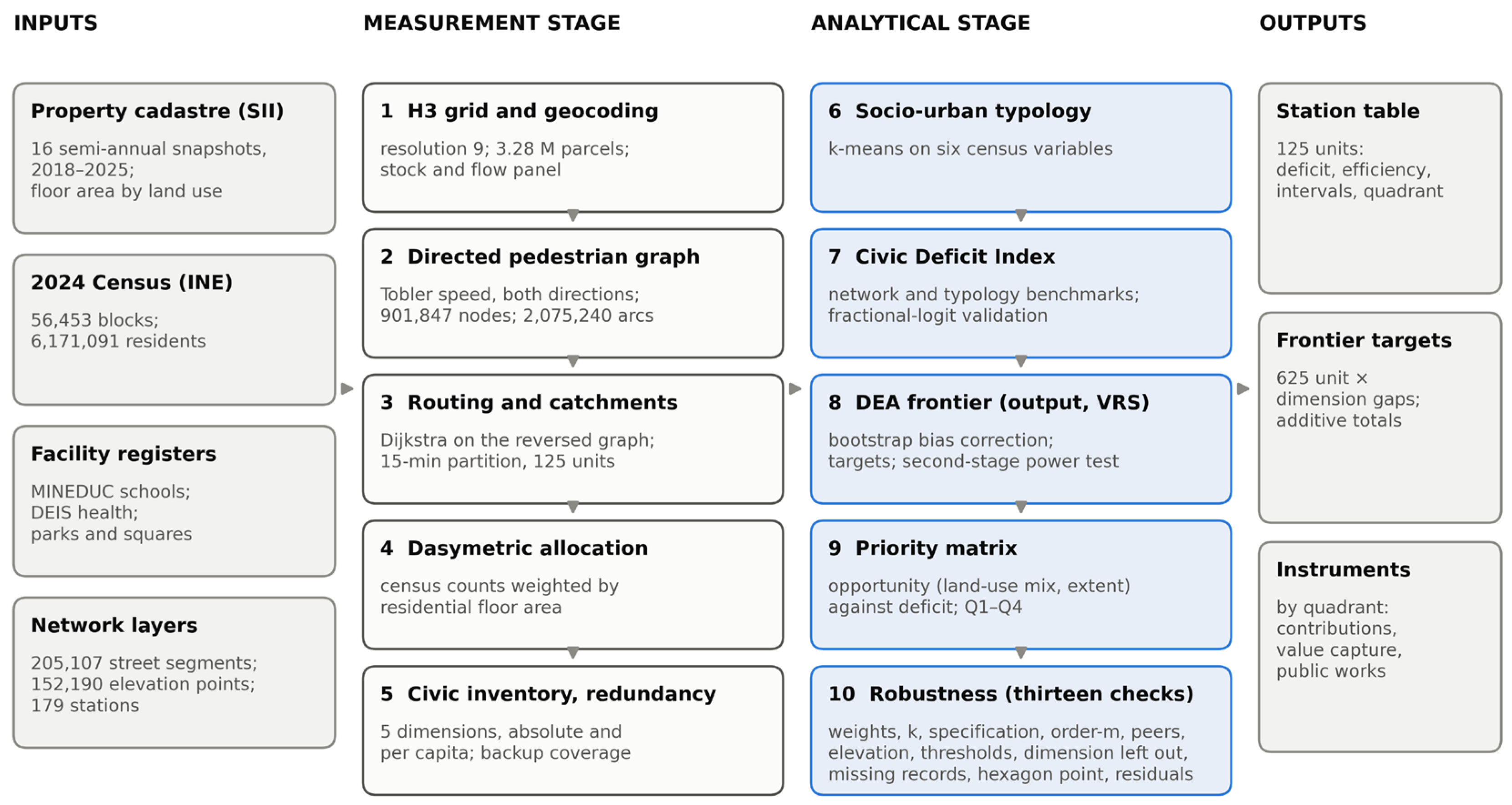
Figure 2.
Santiago Metro network by line and operating status: 125 operating station sites on seven lines (L1–L6 and L4A) and 54 planned stations on Lines 7, 8 and 9 and the airport line (LA). Basemap: Esri World Imagery.
Figure 2.
Santiago Metro network by line and operating status: 125 operating station sites on seven lines (L1–L6 and L4A) and 54 planned stations on Lines 7, 8 and 9 and the airport line (LA). Basemap: Esri World Imagery.
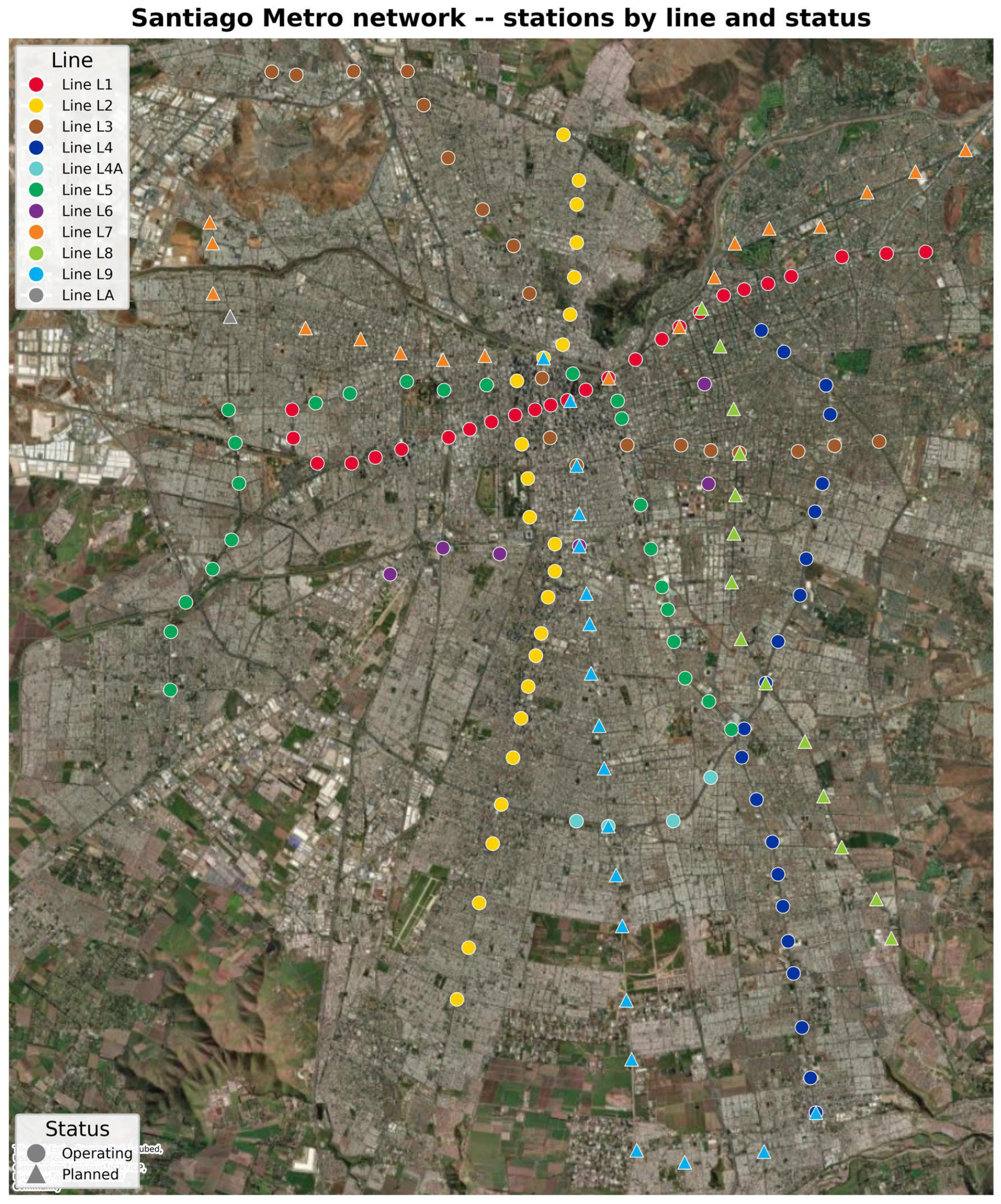
Figure 3.
Walking time from each hexagon to the nearest operating station, on the directed, slope-sensitive pedestrian network. Red dots mark stations; hexagons with no network route within 50 min carry the flagged straight-line estimate. Basemap: Esri World Imagery.
Figure 3.
Walking time from each hexagon to the nearest operating station, on the directed, slope-sensitive pedestrian network. Red dots mark stations; hexagons with no network route within 50 min carry the flagged straight-line estimate. Basemap: Esri World Imagery.
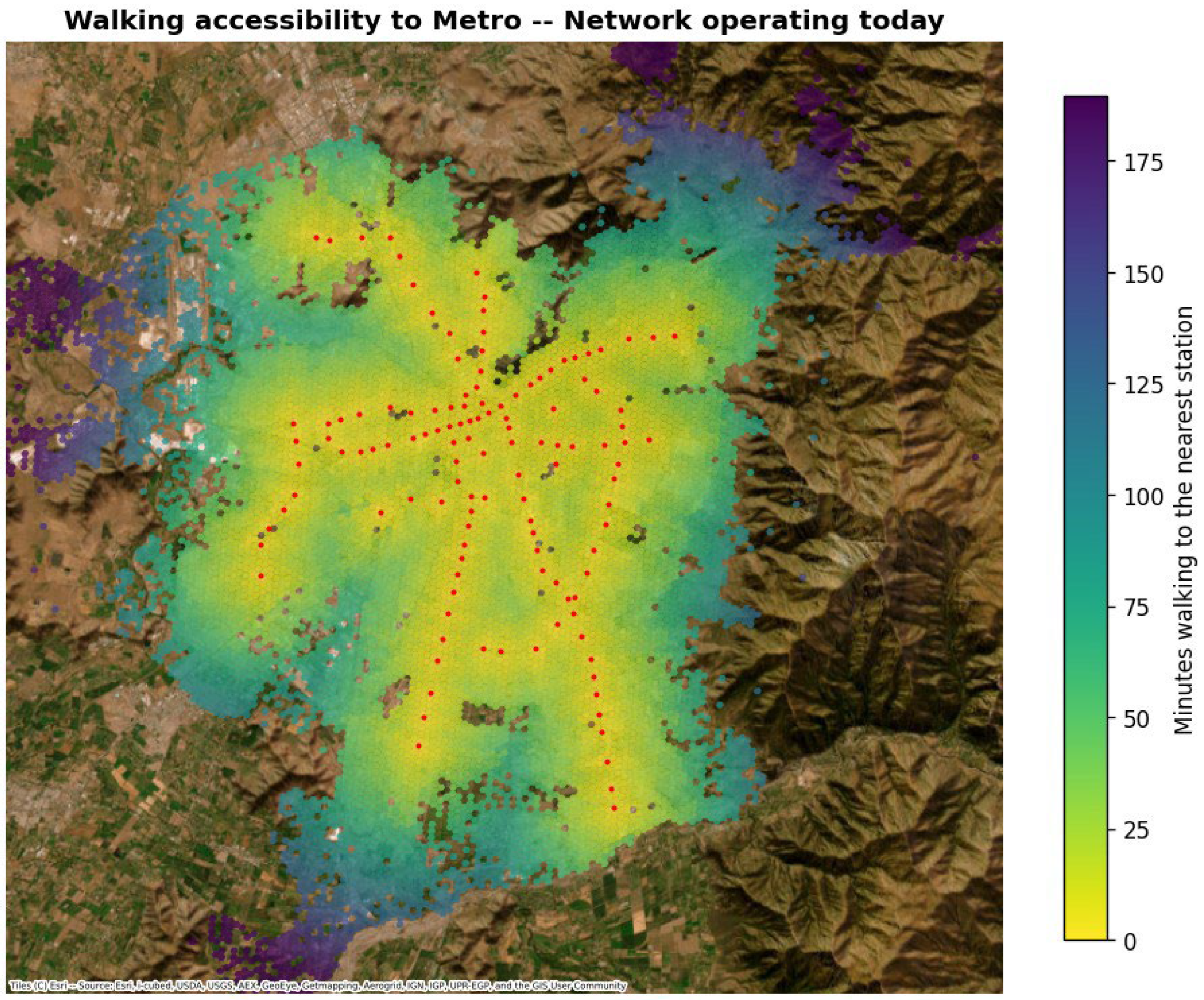
Figure 4.
Redundancy of walking access: share of each catchment’s residents who cannot reach a second station within 15 min (L(s)). Basemap: Esri World Imagery.
Figure 4.
Redundancy of walking access: share of each catchment’s residents who cannot reach a second station within 15 min (L(s)). Basemap: Esri World Imagery.
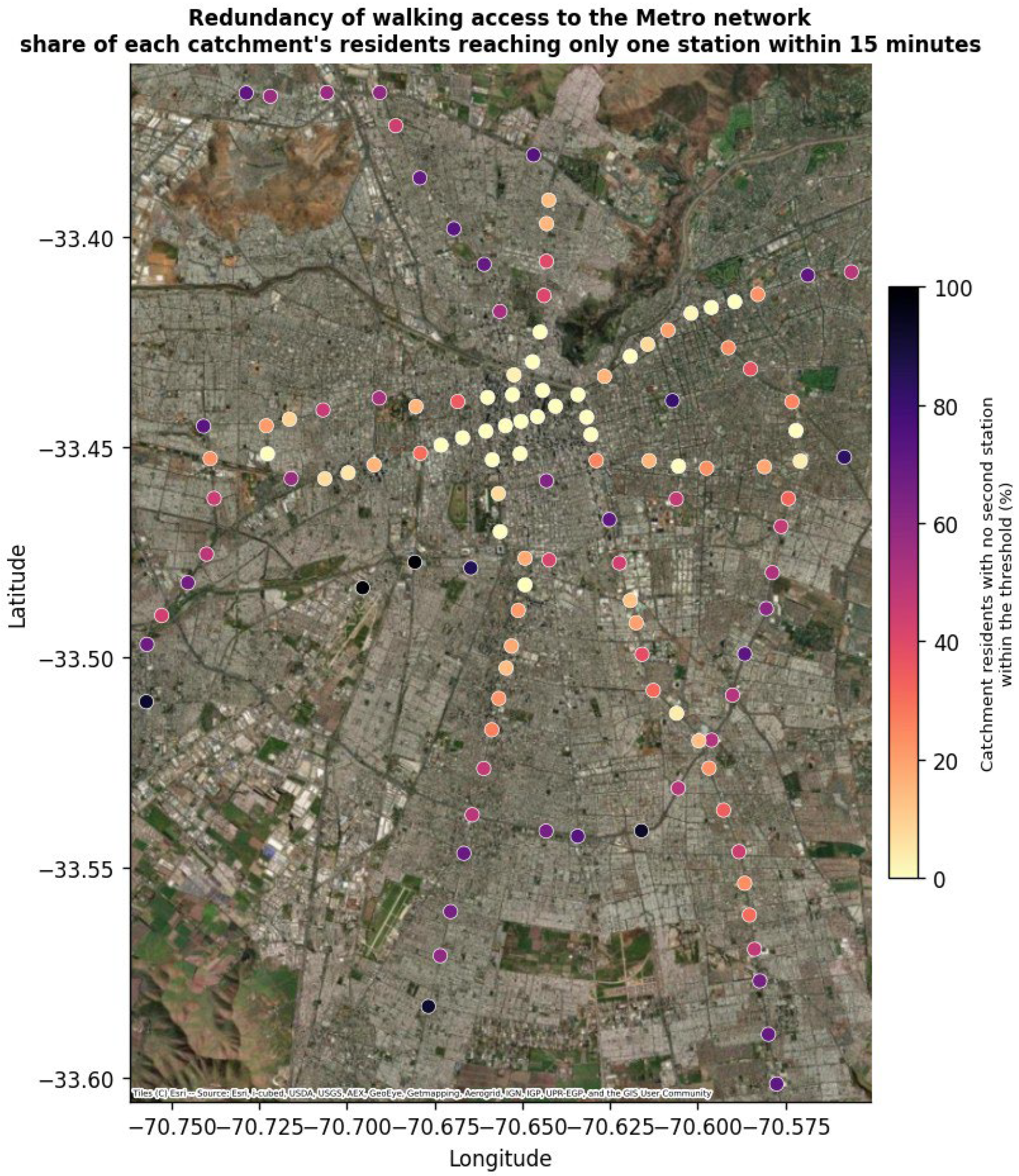
Figure 5.
Housing-deficit rate and mean civic deficit by socio-urban typology, under the network benchmark (CDI-G) and the typology benchmark (CDI-S).
Figure 5.
Housing-deficit rate and mean civic deficit by socio-urban typology, under the network benchmark (CDI-G) and the typology benchmark (CDI-S).
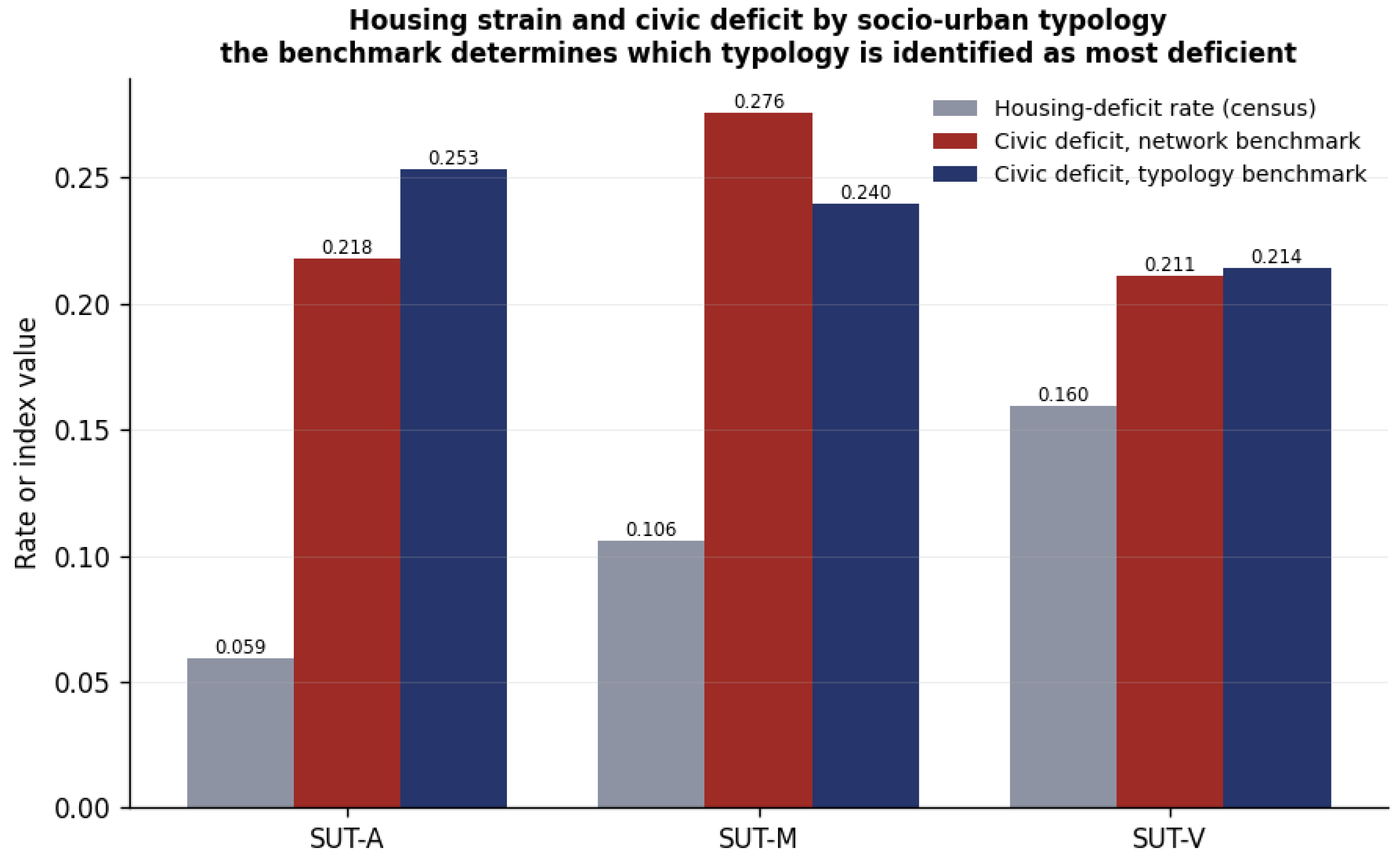
Figure 6.
Output-oriented technical efficiency of the thirty least efficient station areas: bias-corrected score (filled marker), uncorrected score (hollow marker) and 95% bootstrap interval (bar).
Figure 6.
Output-oriented technical efficiency of the thirty least efficient station areas: bias-corrected score (filled marker), uncorrected score (hollow marker) and 95% bootstrap interval (bar).
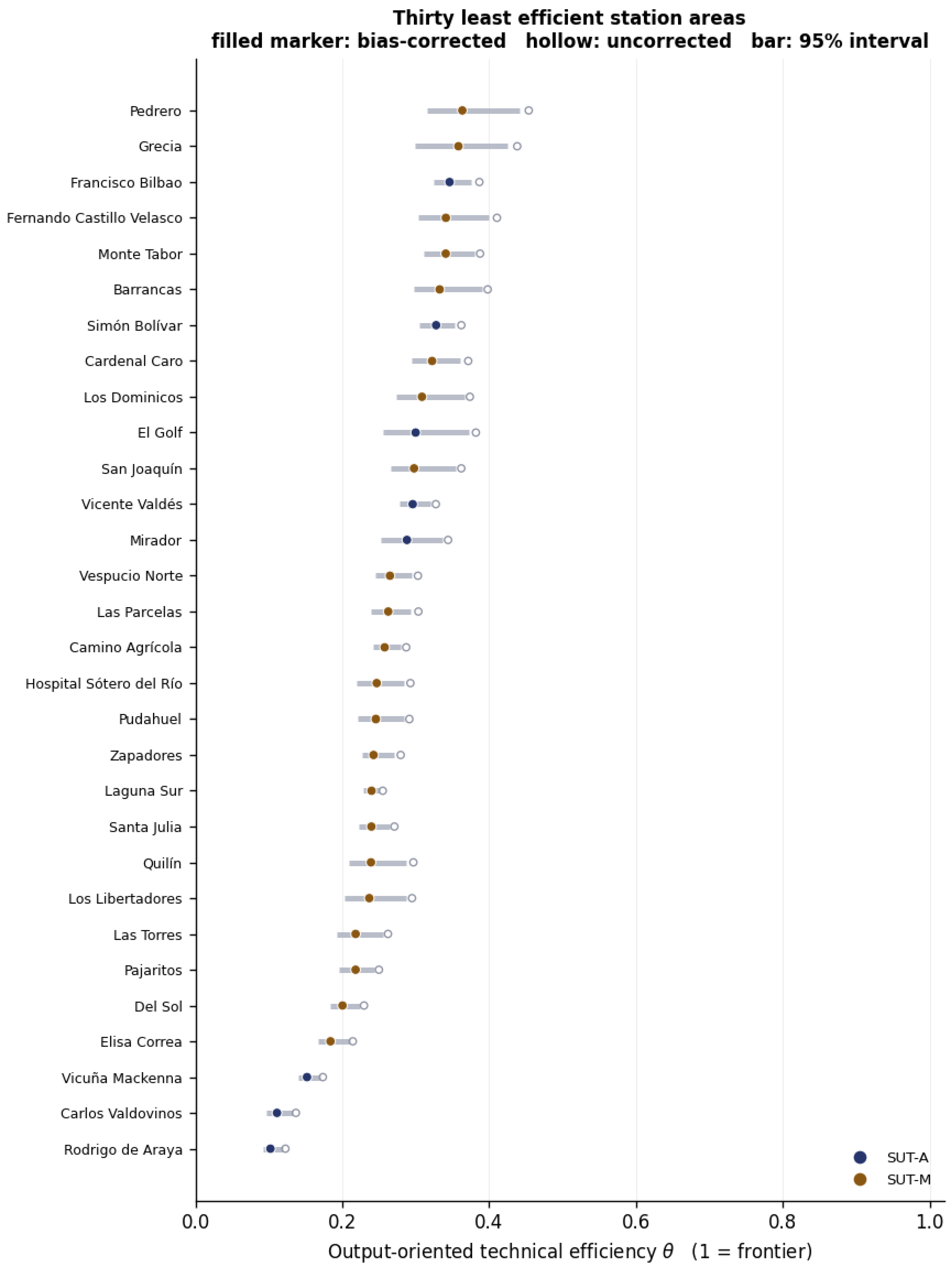
Figure 7.
Technical efficiency (variable returns) against scale efficiency for the 125 station areas. Dashed lines at 0.90 separate provision gaps (upper left), scale gaps (lower right) and both (lower left).
Figure 7.
Technical efficiency (variable returns) against scale efficiency for the 125 station areas. Dashed lines at 0.90 separate provision gaps (upper left), scale gaps (lower right) and both (lower left).
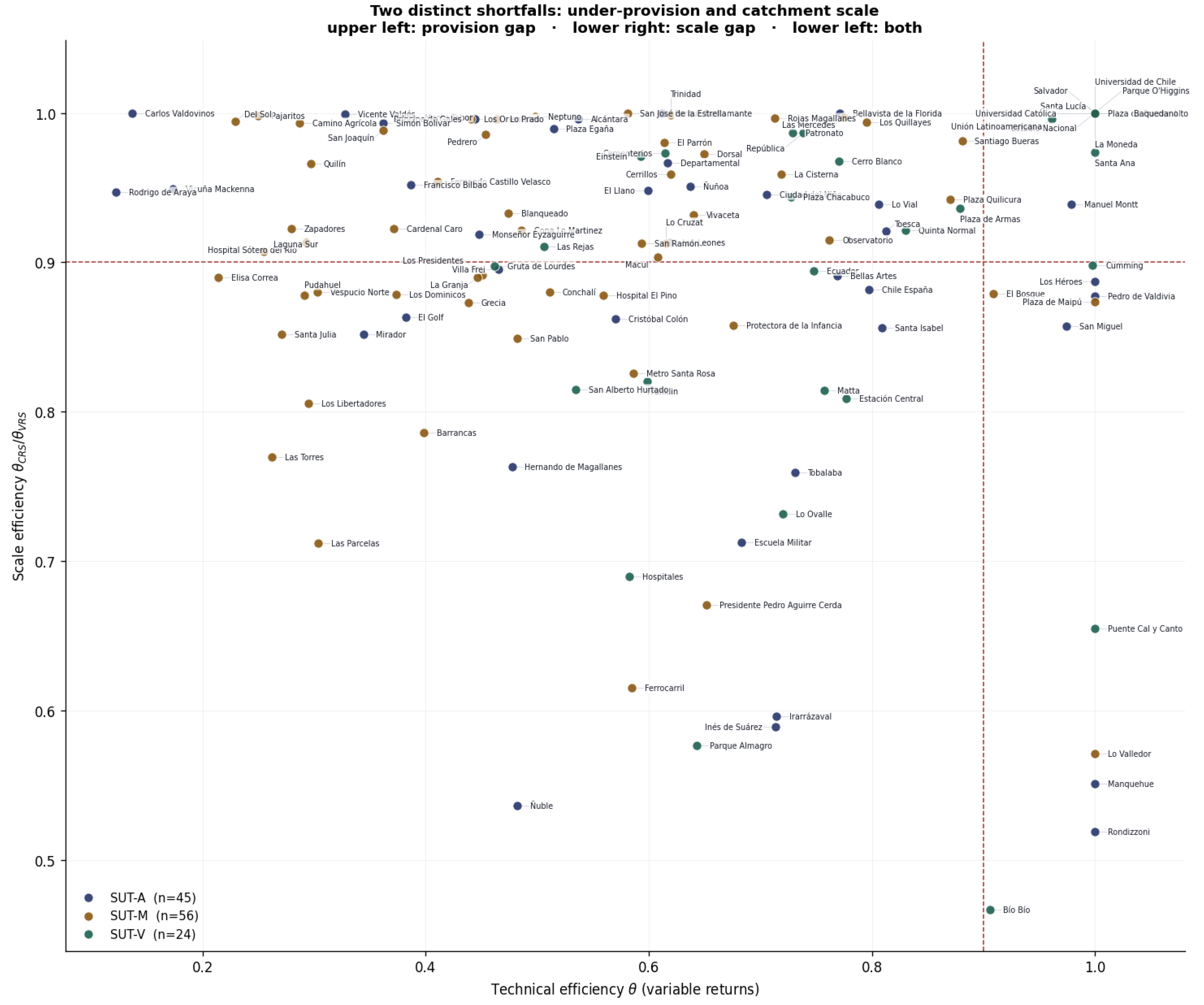
Figure 9.
Priority matrix: structural opportunity (horizontal axis) against the percentile of CDI-G (vertical axis), split at the network median of each axis (49.8 and 50.4). Labels mark the five highest priority indices, the station areas in the worst decile of both measures and the extremes of each axis; Figure S19 names all 125 and Figure S20 maps the quadrants.
Figure 9.
Priority matrix: structural opportunity (horizontal axis) against the percentile of CDI-G (vertical axis), split at the network median of each axis (49.8 and 50.4). Labels mark the five highest priority indices, the station areas in the worst decile of both measures and the extremes of each axis; Figure S19 names all 125 and Figure S20 maps the quadrants.
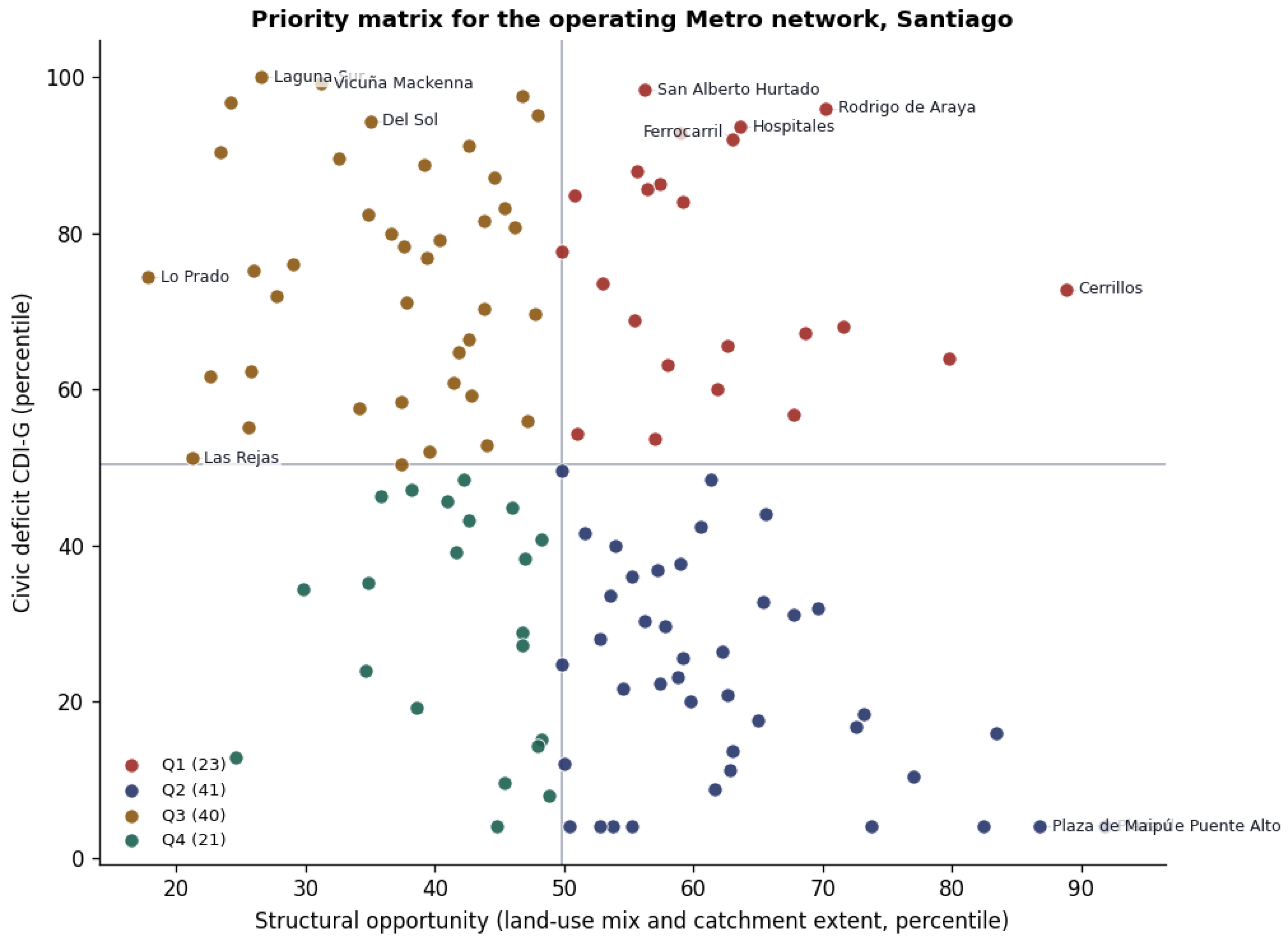
Table 1.
Data sources.
| Dataset | Source | Use | Records in the study area |
| Property cadastre (construction lines, property rolls) | SII [60]; 16 semi-annual snapshots, 2018–2025 | Floor area by land use; dasymetric weight; sports and commerce dimensions; land-use mix | 2,167,716 residential parcels (2025, second half) |
| Parcel geocoding | Author’s geocoding of the cadastre (2026, first half) and a parcel layer (c. 2022) | Parcel-to-hexagon mapping | 3,279,846 parcels; 49,447 blocks (fallback) |
| Population and Housing Census 2024 | INE [59] | Population, dwellings, housing strain, tenure, age, employment, commuting mode | 56,453 blocks; 6,171,091 residents |
| Schools | MINEDUC [63] | Education dimension | 2550 operating schools |
| Health establishments | DEIS–MINSAL [64] | Health dimension (all levels of care) | 884 operating establishments |
| Green space | OpenStreetMap parks and squares, extracted with Overpass Turbo [66] | Green-space dimension | 4400 geometries (26 points); 29.3 km² |
| Street network and elevation | OpenStreetMap street centrelines and elevation points, extracted with Overpass Turbo [66] | Pedestrian graph and slopes | 205,107 segments; 152,190 points |
| Metro stations | Registry compiled by the author from public information | Location, line and status | 179 stations (125 operating) |
SII, Servicio de Impuestos Internos; INE, Instituto Nacional de Estadísticas; MINEDUC, Ministerio de Educación; DEIS, Departamento de Estadísticas e Información de Salud; MINSAL, Ministerio de Salud.
Table 2.
Civic dimensions and their two forms.
| Dimension | Source | Absolute quantity (DEA output) | Per-capita rate (CDI) |
| Sports and recreation | SII cadastre, land use D | Floor area (m²) | m² per resident |
| Local commerce | SII cadastre, land use C | Premises | Premises per 1000 residents |
| Health establishments | DEIS–MINSAL | Establishments | Establishments per 10,000 residents |
| Green space | Parks and squares layer | Area (m²) | m² per resident |
| Education | MINEDUC | Schools | Schools per 100 residents aged 6–17 |
DEA, data envelopment analysis; CDI, Civic Deficit Index. Quantities are sums over the hexagons of each partitioned catchment; rates are ratios of sums.
Table 3.
Walking-access coverage by network scenario and time threshold.
| Scenario | Threshold | Hexagons, all (%) ¹ | Hexagons, shared (%) ² | Population, shared (%) ² | Network-routed pairs (%) ³ |
| Operating network | 15 min | 24.0 | 31.0 | 42.3 | 99.6 |
| 30 min | 43.0 | 54.9 | 70.9 | 99.7 | |
| 45 min | 56.9 | 70.6 | 85.0 | 99.6 | |
| Operating + planned | 15 min | 31.9 | 40.9 | 53.6 | 99.6 |
| 30 min | 52.1 | 65.0 | 80.6 | 99.4 | |
| 45 min | 66.0 | 78.8 | 90.8 | 99.2 |
¹ Share of the 9851 hexagons with at least one geocoded parcel. ² Share of the 7512 hexagons with both an access record and census population (6,164,096 residents, 99.9% of the census population on the grid). ³ Share of hexagon–station pairs within the threshold obtained by network routing rather than by the straight-line fallback.
Table 4.
Per-capita civic provision across the 125 station areas.
| Dimension | Unit | P10 | P25 | Median | P75 | P90 | CV | Zeros ¹ |
| Sports and recreation | m² per resident | 0.002 | 0.025 | 0.083 | 0.218 | 0.465 | 1.926 | 9 |
| Local commerce | premises per 1000 residents | 5.99 | 8.98 | 14.64 | 27.44 | 80.67 | 1.602 | 0 |
| Health establishments | per 10,000 residents | 0.00 | 0.71 | 1.39 | 2.59 | 6.17 | 1.470 | 18 |
| Green space | m² per resident | 0.68 | 1.19 | 2.33 | 3.90 | 7.74 | 1.505 | 1 |
| Education | schools per 100 residents aged 6–17 | 0.16 | 0.25 | 0.37 | 0.52 | 0.64 | 0.628 | 1 |
P10–P90, percentiles; CV, coefficient of variation. ¹ Station areas with no supply on the dimension. The medians are the CDI-G benchmarks. Distributions are shown in Figure S7–S11.
Table 5.
The ten station areas with the highest CDI-G.
| Station area | Line | Typology | CDI-G | CDI-S | Quadrant ¹ |
| Laguna Sur | L5 | SUT-M | 0.673 | 0.631 | Q3 |
| Vicuña Mackenna | L4 | SUT-A | 0.636 | 0.722 | Q3 |
| San Alberto Hurtado | L1 | SUT-V | 0.603 | 0.619 | Q1 |
| Lo Valledor | L6 | SUT-M | 0.600 | 0.600 | Q3 |
| Vicente Valdés | L4 | SUT-A | 0.564 | 0.631 | Q3 |
| Rodrigo de Araya | L5 | SUT-A | 0.564 | 0.583 | Q1 |
| Las Parcelas | L5 | SUT-M | 0.562 | 0.523 | Q3 |
| Del Sol | L5 | SUT-M | 0.550 | 0.505 | Q3 |
| Hospitales | L3 | SUT-V | 0.539 | 0.570 | Q1 |
| Irarrázaval | L3 | SUT-A | 0.501 | 0.553 | Q1 |
¹ Priority quadrant (Section 3.6). Bold: station areas in the worst decile of both CDI-G and the bias-corrected frontier score.
Table 6.
Fractional-response (logit) model of the active-commuting share.
| Covariate | Coefficient | Robust SE | z | p | AME (pp) |
| Intercept | −1.941 | 0.857 | −2.3 | 0.023 | — |
| CDI-G (standardised) | −0.228 | 0.024 | −9.4 | <0.001 | −2.65 |
| IST-2024 | 0.092 | 0.197 | 0.5 | 0.640 | 1.07 |
| Log residential density | 0.065 | 0.087 | 0.8 | 0.453 | 0.76 |
| Distance to the centre (km) | −0.076 | 0.013 | −6.0 | <0.001 | −0.88 |
| SUT-M (ref. SUT-A) | −0.051 | 0.118 | −0.4 | 0.666 | −0.59 |
| SUT-V (ref. SUT-A) | −0.017 | 0.120 | −0.1 | 0.889 | −0.19 |
n = 125, weighted by the number of commuters; Bernoulli quasi-maximum likelihood with HC0 robust standard errors (SE). AME, average marginal effect in percentage points (pp) per unit of the covariate (per standard deviation for CDI-G). Deviance pseudo-R² = 0.616; correlation between observed and fitted shares = 0.787 (Figure S12).
Disclaimer/Publisher’s Note: The statements, opinions and data contained in all publications are solely those of the individual author(s) and contributor(s) and not of MDPI and/or the editor(s). MDPI and/or the editor(s) disclaim responsibility for any injury to people or property resulting from any ideas, methods, instructions or products referred to in the content. |
© 2026 by the authors. Licensee MDPI, Basel, Switzerland. This article is an open access article distributed under the terms and conditions of the Creative Commons Attribution (CC BY) license (http://creativecommons.org/licenses/by/4.0/).
Copyright: This open access article is published under a Creative Commons CC BY 4.0 license, which permit the free download, distribution, and reuse, provided that the author and preprint are cited in any reuse.