Non-Abelian M-Event Dynamics on the Physical–Observation State Bundle

1. Introduction

Returning an experiment to the same physical preparation and observation conditions restores its single-event probabilities. It does not, by itself, determine how the next record is related to the last. The M-event model follows the variable that selects each event and asks what remains of its motion when the observable conditions return.

In PODA, a physical state x and an observation state s jointly describe the objective conditions under which a fact forms [1]. Their admissible values and record probabilities satisfy

$$b=(x,s)\in \mathcal{B}\subseteq \mathcal{X}\times \mathcal{S},K_y\left(b\right)\ge 0,\sum _y{K}_y\left(b\right)=1.$$

(1)

In the quantum representation,

$$K_y(x,s)=Tr\left[{\rho }_x{E}_y^{\left(s\right)}\right].$$

(2)

The observation state describes the objective conditions under which a record forms, independently of anyone’s attention or knowledge. The probability law depends on both x and s.

Here x is the physical state, s the objective conditions of fact formation, and y the resulting event. The kernel specifies its distribution at fixed $(x,s)$. The fiber variable supplies the position that selects a particular event, whose average must agree with that kernel. The kernel fixes proportions, the cells specify the decision, and transport carries the position used by that decision from one set of conditions to the next.

The $U\left(1\right)$ construction [2] attaches a circle to each joint state. The circle is divided into event cells of normalized length $K_y\left(b\right)$; the cell occupied by a point selects the record. A connection transports that point as $(x,s)$ changes. Uniform initial phases reproduce the Born distribution. When readout retains the phase, later events depend on the path already travelled. The original periodic response fixes a phase fingerprint, ${\kappa }_{\mathrm{M}}=0.03080966337\dots$, from which this dependence can be calculated.

The circle imposes a restriction. Take two closed suboperations that return to the same base point and induce fixed transports $U_a=e^{i{\varphi }_a}$ and $U_b=e^{i{\varphi }_b}$ on the same fiber. Then

$$U_b{U}_a=U_a{U}_b=e^{i({\varphi }_a+{\varphi }_b)},U_b^{-1}{U}_a^{-1}{U}_b{U}_a=1.$$

(3)

Interchanging these transports leaves the endpoint unchanged, and their commutator contributes no phase. A $U\left(1\right)$ connection can distinguish paths by their accumulated phases, but two fixed translations on its fiber always commute. Internal motions with a nontrivial commutator therefore require more than a circle coordinate.

The larger fiber must still reproduce the event probabilities. A nontrivial compact connected group has normalized, atomless Haar measure, so any finite probability distribution can be represented by cell volumes. A non-Abelian group also admits nontrivial commutators. The original M-event paper proposed this extension. We derive its coupled dynamics and calculate the record correlations for a definite noncommuting transport.

Scalar and matrix transport have a familiar precedent in quantum dynamics: Berry’s adiabatic phase [3] and the noncommuting transport of Wilczek and Zee [4], both introduced in 1984. Here the transported variable is the event selector. The cell it occupies determines a record, and its motion follows from the M-event action on the dual-axis state space.

A matrix selector also brings a rotating conjugate charge. Its rotation can change the force on the observation coordinate, so the scalar response cannot simply be inserted unchanged into a sequence of matrix operations. In the $U\left(1\right)\times SU\left(2\right)$ realization derived below, a central charge sustains the M response while the matrix coupling changes direction. Four such motions form a commutator. For balanced hemisphere cells on the full $SU\left(2\right)$ group, its conjugacy angle determines the event-mismatch probability exactly. Independent Haar preparation preserves the single-event Born law; the ordering effect appears in the relation between records.

The original free orbit is unique but unstable. A periodic potential allowed by the same action preserves the orbit and its phase while making deviations obey an exact harmonic equation. A further apparatus interaction writes the hemisphere coordinate into a retained record. For zero initial pointer and record momenta, two additional response periods restore both the pointer and the $SU\left(2\right)$ selector. This classical construction supplies the common return assumed in the recurrence calculation. Throughout, the groups are nontrivial compact connected finite-dimensional Lie groups. Their infinitely many elements do not imply an infinite-dimensional group.

2. Event Geometry on Compact Fibers

At each base point the kernel gives the probability of every record, and the selector determines which record occurs. Let $P\to \mathcal{B}$ be a principal bundle with nontrivial compact connected finite-dimensional Lie group G. Its fiber over b contains the possible selector states for those physical–observation conditions. The fiber is a torsor: group translations are defined without choosing a preferred origin. Normalized Haar measure [5] gives it an intrinsic probability measure ${\mu }_b$, preserved by both left and right translations because G is compact.

A record is formed when the selector lies in the corresponding region of the fiber. The volume of that region must agree with the probability already assigned by the physical–observation kernel.

Definition 1

(Event partition). A finite event partition is a measurable family of fiber subsets $\left\{{\mathcal{C}}_y\left(b\right)\right\}$ satisfying

$$P_b=\underset{y}{⨆}{\mathcal{C}}_y\left(b\right),{\mu }_b\left({\mathcal{C}}_y\left(b\right)\right)=K_y\left(b\right).$$

(4)

The event is $Y(b,p)=y$ when $p\in {\mathcal{C}}_y\left(b\right)$. A fixed measurable tie rule assigns any null boundaries, so every selector state has a definite record.

Atomlessness of Haar measure ensures that such cells exist for arbitrary finite record probabilities.

Theorem 1

(Compact-group event lift). Suppose $P\to \mathcal{B}$ admits a measurable section and K is a measurable finite kernel. An event partition satisfying Equation (4) then exists, and its Haar reduction is K.

Proof. 

If a point of G had Haar mass $a>0$, invariance would give the same mass to every translated point. Arbitrarily many distinct points would then have total mass greater than one. Thus Haar measure has no point masses. A compact Lie group is a standard Borel space, on which every measure atom contains a point atom; Haar measure is therefore atomless. There is consequently a measurable uniform coordinate $r:G\to [0,1)$, which may be extended measurably over a null exceptional set. With a measurable section chosen, define

$$t_j\left(b\right)=\sum _{i\le j}{K}_i\left(b\right),C_j\left(b\right)=\{g:t_{j-1}\left(b\right)\le r\left(g\right)<t_j\left(b\right)\}.$$

(5)

Each cell is jointly measurable and has Haar measure $K_j\left(b\right)$. The chosen section identifies these coordinate cells with subsets of $P_b$. Their indicator functions define the records, and their integrals reproduce the kernel.    □

A second-countable smooth principal bundle has the required measurable section. Choose a countable family of local trivializations and, at each base point, use the first available local section. No globally smooth choice of cell boundaries is needed. The kernel K fixes their volumes; their shapes and positions specify further properties of the apparatus.

The physical record cannot depend on the frame used to describe the selector. Under a change of local frame, its coordinate and the cell coordinates transform together:

$$g^{\prime }=h{\left(b\right)}^{-1}g,C_y^{\prime }\left(b\right)=h{\left(b\right)}^{-1}{C}_y\left(b\right).$$

(6)

The same selector remains in the same physical cell, and Haar invariance preserves the cell volume. A threshold chosen independently in each chart would lack this property. Requiring each coordinate cell to remain fixed under all group translations would be too restrictive: transitivity leaves only the empty cell and the whole fiber.

On a finite group, each point has positive Haar mass and cell probabilities are restricted to sums of these masses. A nontrivial compact connected group admits every finite Born distribution. A physical realization must supply a fiber variable, its event partition and a law of transport. The action in the next section supplies that law.

3. Variational Dynamics on the Two-Axis Base

The physical state and the observation state vary along the two tangent directions of the base. On a regular part of $\mathcal{B}$, write

$$T_b\mathcal{B}=H_b^X\oplus H_b^S.$$

(7)

An open product sector has this splitting directly. For a constrained domain, it is a regular splitting of the admissible variations that is assumed; the constraint itself need not provide one. Choose a faithful finite-dimensional unitary representation of G [6]. In this representation the connection $\mathcal{A}={\mathcal{A}}_i\mathrm{d}{b}^i$ is anti-Hermitian. Equip the Lie algebra with a positive Ad-invariant inner product, and replace the scalar charge of the M-event action by a Lie-algebra-valued charge Q, with units of action. The action takes the form

$$S[b,g,Q]=\int \left\{L_0(b,\dot{b})+〈Q,\dot{g}{g}^{-1}+{\mathcal{A}}_i\left(b\right){\dot{b}}^i〉\right\}\mathrm{d}t.$$

(8)

The first term governs the base motion; the second couples it to the selector through the connection. The coordinate g belongs to the fiber over $(x,s)$ and introduces no third base axis.

With the frame convention of Equation (6), the connection and charge obey

$${\mathcal{A}}^{\prime }=h^{-1}\mathcal{A}h+h^{-1}\mathrm{d}h,Q^{\prime }=h^{-1}Qh.$$

(9)

Both entries of the inner product in Equation (8) transform by conjugation. Its Ad invariance therefore makes the action independent of the group frame.

Theorem 2

(Coupled selector equations). Fixed-endpoint variations of $b,g$ and compactly supported variations of Q yield

$$\begin{array}{cccc}\hfill \dot{g}& =-{\mathcal{A}}_{t}g,\hfill & \hfill \dot{Q}+[{\mathcal{A}}_t,Q]& =0,\hfill \end{array}$$

(10)

$$\begin{array}{cccc}\hfill {\mathcal{E}}_i\left(L_0\right)-〈Q,{\mathcal{F}}_{ij}〉{\dot{b}}^j& =0,\hfill & \hfill \mathcal{F}& =\mathrm{d}\mathcal{A}+\mathcal{A}\wedge \mathcal{A},\hfill \end{array}$$

(11)

where ${\mathcal{A}}_t={\mathcal{A}}_i{\dot{b}}^i$ and ${\mathcal{E}}_i\left(L_0\right)={\displaystyle \frac{\mathrm{d}}{\mathrm{d}t}}{\displaystyle \frac{\partial L_0}{\partial {\dot{b}}^i}}-{\displaystyle \frac{\partial L_0}{\partial b^i}}$.

Proof. 

Varying Q imposes parallel transport of g, the first equation in Equation (10). To vary the selector, set $\xi =\dot{g}{g}^{-1}$ and $\eta =\delta g{g}^{-1}$. Differentiating these expressions gives

$$\delta \xi =\dot{\eta }-[\xi ,\eta ].$$

(12)

Integration by parts, together with invariance of the inner product, gives $\dot{Q}=[\xi ,Q]$. Substitution of $\xi =-{\mathcal{A}}_t$ yields the charge equation. The base variation contributes, in addition to ${\mathcal{E}}_i\left(L_0\right)$,

$$〈\dot{Q},{\mathcal{A}}_i〉+〈Q,{\partial }_j{\mathcal{A}}_i-{\partial }_i{\mathcal{A}}_j〉{\dot{b}}^j.$$

(13)

Using the charge equation in the first term gives $〈\dot{Q},{\mathcal{A}}_i〉=-〈Q,[{\mathcal{A}}_i,{\mathcal{A}}_j]〉{\dot{b}}^j$. The derivative and commutator terms combine into $-〈Q,{\mathcal{F}}_{ij}〉{\dot{b}}^j$, which proves Equation (11).    □

The action therefore determines selector transport, charge rotation and the force on the base together. To recover the Abelian equations, set $g=e^{i\chi }$, $\mathcal{A}=-ia$ and $Q=iq$, with $〈iq,i\omega 〉=q\omega$. Then

$$S=\int \{L_0+q(\dot{\chi }-a_i{\dot{b}}^i)\}\mathrm{d}t,$$

(14)

and the force equation becomes ${\mathcal{E}}_i\left(L_0\right)+q{\left(\mathrm{d}a\right)}_{ij}{\dot{b}}^j=0$. These are the transport and force of the original M-event action, with unchanged conventions.

In coordinates $(x^{\mu },s^a)$, the observation component of the force equation is

$${\mathcal{E}}_a\left(L_0\right)-〈Q,{\mathcal{F}}_{a\mu }〉{\dot{x}}^{\mu }-〈Q,{\mathcal{F}}_{ab}〉{\dot{s}}^b=0.$$

(15)

The first curvature term couples the observation response to motion along the physical axis. Its mixed curvature is

$${\mathcal{F}}_{\mu a}={\partial }_{\mu }{\mathcal{A}}_a-{\partial }_a{\mathcal{A}}_{\mu }+[{\mathcal{A}}_{\mu },{\mathcal{A}}_a].$$

(16)

For an infinitesimal mixed loop, this curvature gives the leading transport difference times the oriented area; finite paths require the full ordered propagator. In the Abelian case the last term vanishes. For a non-Abelian connection it can produce mixed curvature even where the coordinate derivatives vanish. At the same time, Q rotates under transport, changing its pairing with the curvature. The force therefore depends both on the local curvature and on the charge brought to that point by the preceding motion.

4. Response Geometry and Ordered Transport

The observation coordinate acquires a metric from the changes it produces in the record probabilities. On a regular identifiable stratum with positive probabilities and full-rank probability differential, this is the Fisher metric of the original observation action:

$$g_{ab}^S(x,s)=\sum _y{\displaystyle \frac{{\partial }_a{K}_y{\partial }_b{K}_y}{K_y}}.$$

(17)

This metric resolves observation directions that change the single-record probabilities. On the unreduced space of observation conditions, a direction V with $\mathrm{d}{K}_y\left(V\right)=0$ for every y instead satisfies

$$g^S(V,V)=\sum _y{\displaystyle \frac{{\left[\mathrm{d}{K}_y\left(V\right)\right]}^2}{K_y}}=0.$$

(18)

Such a direction need not be irrelevant to an event history. Turning a hemisphere anchor without changing its volume, or changing the direction of a matrix coupling, can preserve the single-event probabilities while altering correlations between records. The cells, connection and apparatus action describe these changes. Their freedom cannot be removed by imposing full rank on a metric obtained from the probabilities alone. The response inertia below is assigned to the identifiable response coordinates; further apparatus variables enter through their separately specified couplings.

Take $L_0=L_X(x,\dot{x})+L_S$, where $L_S={\mathcal{I}}_S{g}_{ab}^S(x,s){\dot{s}}^a{\dot{s}}^b/2-V(x,s)$. The momentum conjugate to $s^a$ is ${\mathcal{I}}_S{g}_{ab}^S{\dot{s}}^b$. As the system moves, both x and s may change the metric. Keeping both derivatives in Equation (15) gives

$$\begin{array}{cc}\hfill {\mathcal{I}}_S\left[g_{ab}^S({\ddot{s}}^b+{\Gamma }_{cd}^b{\dot{s}}^c{\dot{s}}^d)+\left({\partial }_{\mu }{g}_{ab}^S\right){\dot{x}}^{\mu }{\dot{s}}^b\right]+{\partial }_{a}V& =〈Q,{\mathcal{F}}_{a\mu }〉{\dot{x}}^{\mu }+〈Q,{\mathcal{F}}_{ab}〉{\dot{s}}^b.\hfill \end{array}$$

(19)

Here ${\Gamma }_{cd}^b$ is the Levi-Civita coefficient of the observation metric at fixed x. The quadratic velocity term supplies the covariant acceleration defined by the observation metric. The mixed derivative accounts for its changing geometry as x moves and vanishes when the metric is independent of x. The right-hand side is the curvature force driving the response. The Levi-Civita connection compares response velocities, whereas $\mathcal{F}$ is the curvature of the connection comparing selector fibers. These are distinct geometric objects even when both contribute to the same observation dynamics.

Once a path $\gamma$ is specified, the selector is obtained by integrating its transport equation:

$$g_1=W_{\gamma }{g}_0,W_{\gamma }=\mathcal{P}exp\left(-{\int }_{\gamma }\mathcal{A}\right).$$

(20)

A later increment acts on the state already reached, so later matrix factors stand to the left. Successive substitution in the integral equation gives

$$W=I-\int {\mathcal{A}}_{t_1}\mathrm{d}{t}_1+{\int }_{t_1>t_2}{\mathcal{A}}_{t_1}{\mathcal{A}}_{t_2}\mathrm{d}{t}_1\mathrm{d}{t}_2+\dots .$$

(21)

where the logarithmic series converges, the first two terms of the Magnus expansion [7] are

$$logW=-\int {\mathcal{A}}_t\mathrm{d}t+{\displaystyle \frac{1}{2}}{\int }_{t_1>t_2}[{\mathcal{A}}_{t_1},{\mathcal{A}}_{t_2}]\mathrm{d}{t}_1\mathrm{d}{t}_2+\dots .$$

(22)

The commutator records the order of the increments. Two paths with the same ordinary connection integral can therefore end at different selector states. This dependence on order, together with charge rotation and the curved response geometry, gives the event dynamics its nonlinearity. The ensemble law, Equation (2), remains linear in the quantum state.

The transport matrix transforms as $W_{\gamma }^{\prime }=h{\left(b_1\right)}^{-1}{W}_{\gamma }h\left(b_0\right)$. For a closed loop, this becomes conjugation. Its trace and conjugacy class consequently have a meaning independent of the frame, whereas a comparison of matrix entries or generator directions uses a common physical frame at the endpoints.

Although the charge affects the base motion, neither equation contains the selector coordinate. This absence is what allows the coupled dynamics to preserve Haar measure.

Theorem 3

(Conditional Haar preservation). A selector initially distributed according to Haar measure, independently of a prescribed base path, remains Haar distributed at the transported endpoint. For the coupled Equations (10) and (11), the same statement holds conditional on all initial base data $(b_0,{\dot{b}}_0)$ and charge $Q_0$ independent of the Haar selector, provided that the initial-value problem has a unique solution.

Proof. 

A fixed left translation preserves Haar measure. In the coupled system, the equations for $(b,Q)$ contain no g. Conditioning on their initial data fixes their unique solution and hence $W_{\gamma }$, independently of $g_0$. The endpoint is therefore a fixed left translate of the initial Haar selector. Integrating the endpoint cell indicator gives $K_y\left(b_1\right)$.    □

The theorem concerns Equation (8) before the selector–pointer interaction is added. The later zero-momentum apparatus preparation removes its added force and preserves the argument. Nonzero apparatus momenta generally make the path selector-dependent, in which case the full device dynamics must be used to determine the distribution.

These independence conditions are physical restrictions on preparation and control. The choice $Q_0={Ad}_{g_0}{Q}_{\mathrm{body}}$ correlates charge and selector; controls that depend on earlier records can likewise make the path depend on the selector. Haar preservation need not hold in either case. Even independent reversible transport only translates a distribution: it does not bring an arbitrary distribution to equilibrium. Conditioning on an outcome restricts the ensemble to its event cell. The theorem thus determines the unconditioned endpoint marginals under the prescribed controls, while outcome-selected subensembles generally have a different measure.

5. Binary Records on the Full $\mathbf{SU}\left(\mathbf{2}\right)$ Fiber

For $SU\left(2\right)$ the relation between transport and two records can be found exactly. Write a group element in quaternion form,

$$u=z_{0}I+i\mathbf{z}·\sigma ,z_0^2+{\left|\mathbf{z}\right|}^2=1.$$

(23)

Haar measure is uniform surface measure on the resulting three-sphere $S^3$. A drawing of $\mathbf{z}$ places this sphere in a three-dimensional ball: an interior point generally has two possible values of $z_0$. The selector thus occupies the full group manifold, distinct from the Bloch sphere that describes a two-state ray.

Let c be a physical anchor at the endpoint, expressed in the same group frame. A balanced binary readout is obtained by dividing the fiber into two hemispheres:

$$C_{+}=\left\{u:{\displaystyle \frac{1}{2}}\Re Tr\left(c^{-1}u\right)\ge 0\right\},C_{-}=SU\left(2\right)\setminus C_{+}.$$

(24)

The two hemispheres have equal Haar volume and hence equal record probabilities. The test is unchanged under $u^{\prime }=h^{-1}u$ and $c^{\prime }=h^{-1}c$, so the anchor defines a physical partition independent of its coordinates. Equal Born weights fix the volumes alone. The hemisphere shape is an additional apparatus property assumed in this realization.

The same geometry also admits unequal binary weights. For a uniform point on $S^3$, the scalar coordinate has density $2\sqrt{1-z^2}/\pi$ on $[-1,1]$, and hence

$$\mu (z_0\ge t)={\displaystyle \frac{arccost-t\sqrt{1-t^2}}{\pi }}.$$

(25)

Varying the cap threshold gives any binary probability. The balanced value $t=0$ has the additional advantage that the correlation under repeated transport can be calculated exactly.

Theorem 4

($SU\left(2\right)$ hemisphere mismatch). Let u be Haar distributed and $W\in SU\left(2\right)$ fixed. Define

$$\alpha \left(W\right)=arccos\left({\displaystyle \frac{1}{2}}TrW\right)\in [0,\pi ].$$

(26)

The hemisphere records formed from u and $Wu$ disagree with probability $\alpha \left(W\right)/\pi$.

Proof. 

For $\alpha =0$ the two records agree, and for $\alpha =\pi$ they are opposite outside the null boundary. For $0<\alpha <\pi$, replace u by $c^{-1}u$. This moves the anchor to the identity and replaces the transported matrix by $\left(c^{-1}Wc\right)u$. Its scalar coordinate is a unit linear form in the four quaternion coordinates. The normal to this form has inner product $\Re Tr\left(W\right)/2$ with the original scalar-coordinate normal, so the angle between the two normals is $\alpha \left(W\right)$. Uniform measure on $S^3$ is invariant under rotations in the plane spanned by them. Conditional on a nonzero projection into this plane, the polar angle is uniform; zero projection has measure zero. The two sign tests differ over a total angle $2\alpha$ out of $2\pi$, giving probability $\alpha /\pi$.    □

The averaging uses the rotational symmetry of Haar measure on the full $S^3$; it requires neither a chosen circle subgroup nor a uniform phase on such a circle.

Now repeat a complete endpoint operation. Assume that transport, readout, and reset together act as $u\mapsto Wu$ on either outcome branch, and that the endpoint anchor and Born law return to their initial values. After N operations, the transport is $W^N$, carrying the same selector to $W^{N}u$. The mismatch theorem gives

$$\begin{array}{cc}\hfill P_{\mathrm{mis}}\left(N\right)& ={\displaystyle \frac{1}{\pi }}arccos[cos\left(N\alpha \right)],\hfill \end{array}$$

(27)

$$\begin{array}{cc}\hfill C_N:=\mathbb{E}\left(Y_0{Y}_N\right)& =1-2P_{\mathrm{mis}}\left(N\right),Y_k\in \{-1,1\}.\hfill \end{array}$$

(28)

The marginal record probability remains one half at every endpoint, while the same transported selector produces correlations between endpoints. If each return instead prepares an independent Haar selector, that correlation is lost and $P_{\mathrm{mis}}\left(N\right)=1/2$ for every $N\ge 1$.

The binary partition also makes the central sign of $SU\left(2\right)$ physically relevant: u and $-u$ occupy opposite hemispheres. Ordinary channel tomography identifies W with $-W$, leaving this sign unresolved. To determine the full matrix, the experiment therefore needs a coherent reference, for example a relative-phase measurement of a controlled matrix operation. A Bloch rotation measured without such a reference determines only the $SO\left(3\right)$ image.

6. A Charged Response and Its Matrix Transport

A numerical event fingerprint requires a definite response orbit. In the scalar M-event model a constant charge drives the observation coordinate around a closed orbit, accumulating phase along it. The same orbit can drive matrix rotations about successive axes, provided that changing the axis leaves the response force unchanged.

An entirely $SU\left(2\right)$ charge would not generally have this property. Its component $〈Q,T〉$ along the active generator sets the response force, and earlier rotations can change that component. Reversing the coupling also reverses a velocity-dependent force without necessarily retracing the motion. A central charge supplies the same response force for every matrix direction, while the traceless connection turns the selector.

For this purpose, take the group and connection in Equation (8) to be

$$G=U\left(1\right)\times SU\left(2\right),g=(e^{i\chi },u),\mathcal{A}=(-ia,-aT\left(\mathbf{n}\right)),T\left(\mathbf{n}\right)=i\mathbf{n}·\sigma ,$$

(29)

where the unit vector $\mathbf{n}$ sets the direction of the applied coupling. The inner product is the product inner product, with $〈X,Y〉=-Tr\left(XY\right)/2$ on the traceless factor. In the chart used for the response motion, the scalar connection is

$$a=f\left(\theta \right)\mathrm{d}\phi ,f\left(\theta \right)={\displaystyle \frac{1-cos\theta }{2}}.$$

(30)

The same one-form a appears in both factors. Its relative normalization is fixed by the way the original phase is represented in the matrix channel. For each fixed direction $\mathbf{n}$, we require a faithful continuous homomorphism ${\rho }_{\mathbf{n}}$ from the circle into $SU\left(2\right)$ and take its differential image as the matrix connection. Successive scalar phase displacements then compose in exactly the same way as their matrix images.

Proposition 1

(Faithful transport of the original phase). A fixed-axis homomorphism of the form

$${\rho }_{\mathbf{n}}\left(e^{i\chi }\right)=exp[i\lambda \chi \mathbf{n}·\sigma ]$$

(31)

is single-valued on $U\left(1\right)$ only when λ is an integer. It is faithful precisely when $\left|\lambda \right|=1$. Choosing the axis orientation fixes $\lambda =1$ and gives $d{\rho }_{\mathbf{n}}(-ia)=-aT\left(\mathbf{n}\right)$.

Proof. 

A full turn of the scalar phase returns to the same point of $U\left(1\right)$. Its matrix image must therefore satisfy $exp(i2\pi \lambda \mathbf{n}·\sigma )=I$, so $\lambda \in \mathbb{Z}$. For $\left|\lambda \right|>1$, the nonzero circle displacement $2\pi /\left|\lambda \right|$ already maps to the identity; for $\lambda =0$, every displacement does so. Only $\left|\lambda \right|=1$ preserves every distinct circle phase. The two remaining choices differ by reversal of $\mathbf{n}$.    □

A faithful circle homomorphism and its differential connection preserve the original phase in each fixed-axis matrix transport. These are assumptions of this realization; the dual-axis structure alone does not impose them. A local coupling ${\mathcal{A}}_{\lambda }=(-ia,-\lambda aT)$ with another real gain is allowed and gives the different fingerprint calculated below. Equation (29) is written in a common calibrated frame. In another gauge its two components obey Equation (9), and need not retain their displayed expression through the same one-form.

In this realization, $\phi \left(t\right)$ is a prescribed physical drive, $\theta \left(t\right)$ is the observation response to be solved for, and $\mathbf{n}\left(t\right)$ is the prescribed direction of an observation-side coupling. The response has the stated inertia; the drive and direction are not assigned additional free equations of motion here. Write the charge as $Q=(iq,Q_s)$ and take $L_S={\mathcal{I}}_S{\dot{\theta }}^2/2$. The driven restriction of Equation (8) becomes

$$S=\int \left\{{\displaystyle \frac{{\mathcal{I}}_S}{2}}{\dot{\theta }}^2+q(\dot{\chi }-f\dot{\phi })+〈Q_s,\dot{u}{u}^{-1}-f\dot{\phi }T\left(\mathbf{n}\right)〉\right\}\mathrm{d}t.$$

(32)

Varying $\theta ,u,\chi$ and the two charge components, with the drive and direction held prescribed, gives transport in both factors and the response equation

$$\ddot{\theta }+{\displaystyle \frac{q+〈Q_s,T\left(\mathbf{n}\right)〉}{2{\mathcal{I}}_S}}sin\theta \dot{\phi }=0.$$

(33)

Thus the charge projection on the active direction changes the observation force. After taking these variations, choose the invariant charge sector $Q_s=0$. The resulting equations are

$$\ddot{\theta }+{\displaystyle \frac{q}{2{\mathcal{I}}_S}}sin\theta \dot{\phi }=0,\dot{\chi }=f\dot{\phi },\dot{u}=f\dot{\phi }T\left(\mathbf{n}\right)u.$$

(34)

The charge q is constant, and conjugation carries $Q_s=0$ into itself. Thus the observation coordinate follows the same equation for every direction $\mathbf{n}$. Changing that direction turns the matrix motion; reversing it reverses the matrix transport without changing the force on $\theta$.

The Hamiltonian makes the relation between force and transport explicit. Put $p_{\theta }={\mathcal{I}}_S\dot{\theta }$ and $J_{\mathbf{n}}=〈Q_s,T\left(\mathbf{n}\right)〉$. The Legendre transform of Equation (32), retaining the group canonical terms, gives

$$H_{\mathrm{eff}}={\displaystyle \frac{p_{\theta }^2}{2{\mathcal{I}}_S}}+f\left(\theta \right)\dot{\phi }[q+J_{\mathbf{n}}].$$

(35)

Differentiation with respect to the response coordinate gives the force, while variation of the charge gives transport. This explains why $Q_s=0$ is imposed after variation: setting it to zero in the action would suppress the matrix transport equation itself.

The condition $Q_s=0$ concerns a classical charge. It removes the traceless reaction force while leaving the $SU\left(2\right)$ representation active. A spin-zero representation would remove the matrix operations themselves. The apparatus therefore needs a separately readable channel that realizes the matrix connection, just as the scalar experiment needs a readable phase channel.

In the common experimental frame the chosen connection has only a $\mathrm{d}\phi$ component; its components along coupling-direction parameters ${\nu }^A$ are specified to be zero. This is a constitutive choice, not a gauge freedom that removes arbitrary components in all directions. If $\mathbf{n}=\mathbf{n}\left(\nu \right)$ is included as an observation-control parameter in the same chart, the mixed curvatures are

$$\begin{array}{cc}\hfill {\mathcal{F}}_{\theta \phi }& =\left(-{\displaystyle \frac{i}{2}}sin\theta ,-{\displaystyle \frac{1}{2}}sin\theta T\left(\mathbf{n}\right)\right),\hfill \\ \hfill {\mathcal{F}}_{{\nu }^A\phi }& =\left(0,-f\left(\theta \right)T\left({\partial }_A\mathbf{n}\right)\right).\hfill \end{array}$$

(36)

Here $\mathcal{A}\wedge \mathcal{A}=0$ in this particular realization, although finite transports about different directions need not commute. The four-block commutator depends on these actual control paths. A passive frame change instead transforms the selector, charge, cells and anchor together and leaves the physical record unchanged. Setting $Q_s=0$ removes its base force, while preserving the matrix connection, its mixed curvature and its transport. Extending the description over the whole response sphere and all coupling directions would require further bundle data. The central $U\left(1\right)$ factor carries the unit-Chern normalization; $SU\left(2\right)$ bundles over $S^2$ are trivial. The product group $U\left(1\right)\times SU\left(2\right)$ is also essential to this description. Its replacement by $U\left(2\right)$ would identify pairs differing in both central and $SU\left(2\right)$ sign, losing the independently defined sign required by hemisphere readout.

6.1. The Closed Response Orbit

The binary probability $p_{+}={sin}^2(\theta /2)$ fixes a particularly simple length element. Substitution into Equation (17) gives $\mathrm{d}{\ell }_S^2=\mathrm{d}{\theta }^2$, so $\theta$ measures Fisher distance along the response. On the reduced selector sphere, rotational invariance and unit-Chern normalization give $\mathrm{d}a=\frac{1}{2}sin\theta \mathrm{d}\theta \wedge \mathrm{d}\phi$. This is the scalar geometry carried into the central factor from the M-event construction.

Let the physical drive make one sinusoidal excursion, $\phi =0.100cos\xi$, where $\xi =\Omega t$, and choose $q/\left({\mathcal{I}}_S\Omega \right)=4$. Requiring the observation coordinate to return to the balanced value $\pi /2$ after one drive period gives

$${\theta }^{\prime \prime }\left(\xi \right)=0.200sin\theta \left(\xi \right)sin\xi ,\theta \left(0\right)=\theta \left(2\pi \right)={\displaystyle \frac{\pi }{2}}.$$

(37)

Thus the coefficient $0.200=0.100\times 4/2$ comes directly from the drive amplitude and the chosen charge-to-inertia frequency ratio. No event probability enters its determination.

Proposition 2

(Unique returning orbit). Equation (37) has a unique solution. It obeys $\theta (2\pi -\xi )=\pi -\theta \left(\xi \right)$ and ${\theta }^{\prime }\left(2\pi \right)={\theta }^{\prime }\left(0\right)$, and stays away from the poles.

Proof. 

With $y=\theta -\pi /2$, the boundary values become zero. The Dirichlet inverse $D^{-2}$ of the second derivative on $[0,2\pi ]$ has supremum norm ${\pi }^2/2$, and hence the integral equation $y=D^{-2}[0.200cosysin\xi ]$ is a contraction with Lipschitz constant $0.1{\pi }^2<1$. Its unique fixed point satisfies ${∥y∥}_{\infty }\le 0.1{\pi }^2<\pi /2$, which keeps the orbit inside the regular chart. Reflection about the midpoint produces another solution of the same boundary-value problem. Uniqueness therefore gives the stated reflection symmetry, and its derivative gives equality of the endpoint velocities.    □

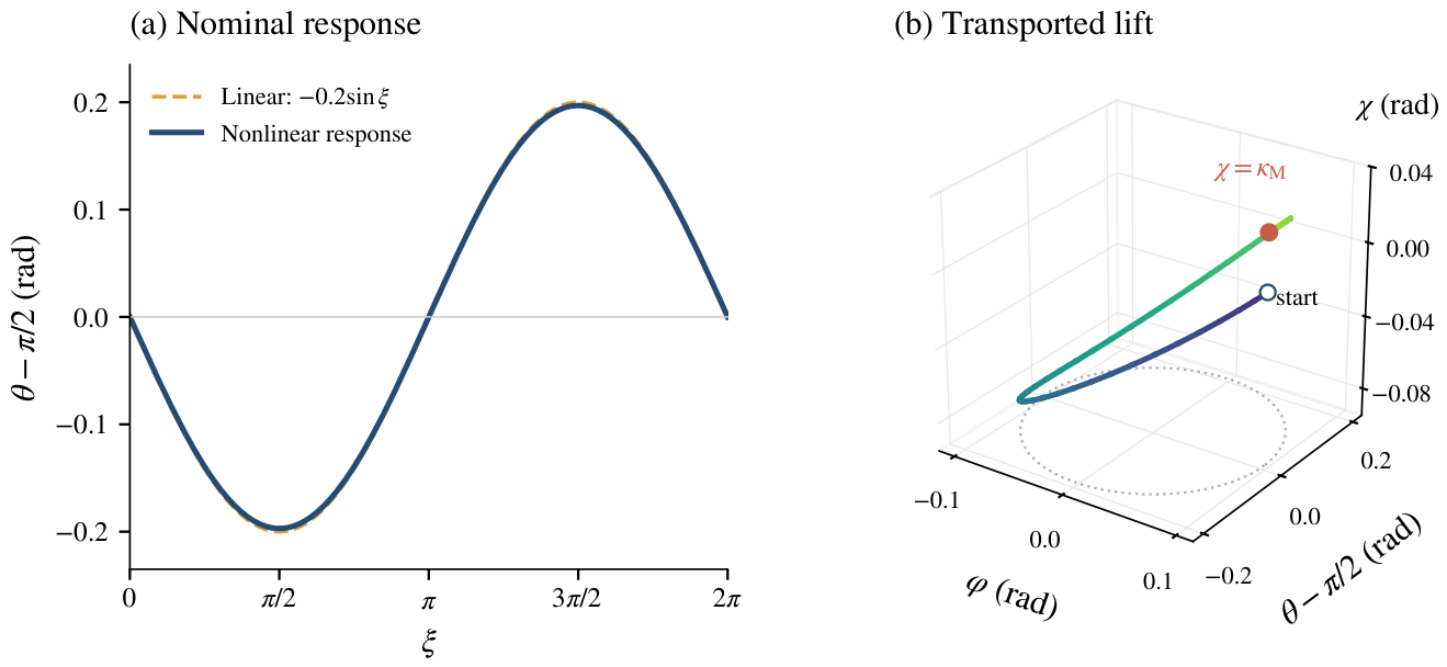
A closed response orbit can leave a nonzero phase. The connection integral gives the dimensionless scalar holonomy

$${\kappa }_{\mathrm{M}}={\int }_0^{2\pi }{\displaystyle \frac{1-cos\theta \left(\xi \right)}{2}}[-0.100sin\xi ]\mathrm{d}\xi =0.03080966336633756\dots .$$

(38)

The orbit starts with slope $-0.19741748313409829\dots$ and departs from $\pi /2$ by at most approximately $0.19698823932244$ radians. Position and velocity both return, so the motion continues periodically with phase ${\kappa }_{\mathrm{M}}$ on each exact repetition. Its usefulness for a long sequence also depends on the motion of nearby trajectories.

Figure 1. A closed response motion and its accumulated phase. The drive and response return to their initial values, closing the base loop. Its three-dimensional lift remains open: the endpoint displacement along the fiber is ${\kappa }_{\mathrm{M}}$. The curves follow from Equation (37) and the connection in Equation (30).

Figure 1. A closed response motion and its accumulated phase. The drive and response return to their initial values, closing the base loop. Its three-dimensional lift remains open: the endpoint displacement along the fiber is ${\kappa }_{\mathrm{M}}$. The curves follow from Equation (37) and the connection in Equation (30).

6.2. Periodic Continuation and Stability

During repeated transport the response must remain near its closed orbit. Let ${\theta }_{*}\left(\xi \right)$ be the periodic continuation of Equation (37), and put ${\eta }_{\mathrm{M}}=0.200$. A small displacement from this free orbit obeys

$$z^{\prime \prime }=c\left(\xi \right)z,c\left(\xi \right)={\eta }_{\mathrm{M}}cos{\theta }_{*}\left(\xi \right)sin\xi .$$

(39)

Its coefficient has a definite sign. The reflection symmetry fixes ${\theta }_{*}\left(\pi \right)=\pi /2$. In the first half-period, $y={\theta }_{*}-\pi /2$ has positive second derivative and zero endpoint values, so $y<0$; in the second half-period its sign is reversed. It follows that $c\left(\xi \right)>0$ except at $0,\pi ,2\pi$.

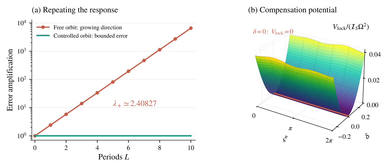
The sign of c determines the stability. For solutions $C,S$ of Equation (39) with initial data $(1,0)$ and $(0,1)$, respectively, one has $C\left(2\pi \right)>1$ and $S^{\prime }\left(2\pi \right)>1$. The constant Wronskian gives a period matrix of determinant one; these inequalities give it a trace greater than two. Its Floquet multipliers [8] are therefore positive reciprocals, with one greater than unity. Numerical integration gives

$$M_{\mathrm{free}}\simeq \left(\begin{array}{cc}1.41175116017& 7.19281552386\\ 0.138060170589& 1.41175116017\end{array}\right),{\lambda }_{+}\simeq 2.40826575527,{\lambda }_{-}\simeq 0.415236565073.$$

(40)

The free orbit is unstable. Over 100 periods the linearized growing component increases by approximately $1.48\times {10}^{38}$; a finite preparation error leaves the linear regime much earlier. Thus the exact orbit fixes a holonomy, but does not by itself provide a stable long sequence.

The response action already allows a scalar potential. One can choose it to preserve the orbit while changing the motion of nearby trajectories. The reference ${\theta }_{*}\left(\xi \right)$ is calculated in advance and checked on a separate response ensemble. The prescribed drive phase $\xi mod2\pi$, an apparatus coordinate on the physical axis, supplies its clock. Application of this potential therefore needs no selector measurement or event-dependent control.

To construct it, measure displacement from the reference by $\delta =\theta -{\theta }_{*}\left(\xi \right)$ and choose a positive dimensionless frequency $\nu$. Set

$$\begin{array}{cc}\hfill V_{\mathrm{lock}}(\theta ,\xi )={\mathcal{I}}_S{\Omega }^2\{& {\eta }_{\mathrm{M}}[cos{\theta }_{*}\left(\xi \right)-cos\theta -sin{\theta }_{*}\left(\xi \right)\delta ]sin\xi \hfill \\ \hfill & +\frac{1}{2}{\nu }^2{\delta }^2\}.\hfill \end{array}$$

(41)

The response Lagrangian in Equation (32) becomes ${\mathcal{I}}_S{\dot{\theta }}^2/2-V_{\mathrm{lock}}$, with unchanged group terms, or equivalently the Hamiltonian in Equation (35) gains $+V_{\mathrm{lock}}$. The construction assumes an apparatus capable of realizing this potential; it does not yet specify a microscopic implementation.

Proposition 3

(Exact bounded response deviation). With the programmed potential (41), every response trajectory in the regular chart satisfies

$${\delta }^{\prime \prime }+{\nu }^2\delta =0.$$

(42)

The nominal orbit and its M-event holonomy remain unchanged. For $\nu =1$, position and velocity errors return after each original response period.

Proof. 

On the reference orbit, both the potential and its $\theta$ derivative vanish. Away from it, differentiation gives

$${\displaystyle \frac{{\partial }_{\theta }{V}_{\mathrm{lock}}}{{\mathcal{I}}_S{\Omega }^2}}={\eta }_{\mathrm{M}}(sin\theta -sin{\theta }_{*})sin\xi +{\nu }^2\delta .$$

(43)

The response equation is therefore

$${\theta }^{\prime \prime }={\eta }_{\mathrm{M}}sin\theta sin\xi -{\displaystyle \frac{{\partial }_{\theta }{V}_{\mathrm{lock}}}{{\mathcal{I}}_S{\Omega }^2}}={\theta }_{*}^{\prime \prime }-{\nu }^2\delta .$$

(44)

Subtracting the reference motion yields Equation (42) exactly, for finite as well as infinitesimal displacements within the chart. At $\nu =1$, the solution is

$$\delta \left(\xi \right)={\delta }_{0}cos\xi +{\delta }_0^{\prime }sin\xi ,\left|\delta \left(\xi \right)\right|\le A_0,A_0=\sqrt{{\delta }_0^2+{\left({\delta }_0^{\prime }\right)}^2}.$$

(45)

The displacement and its velocity repeat after $2\pi$. On the nominal orbit, neither the path nor the connection has changed, so the accumulated phase is still ${\kappa }_{\mathrm{M}}$.    □

This is neutral stability: the phase-space error keeps a constant amplitude. There is no attraction to the reference orbit. The potential contains no selector coordinate, so the conditional Haar argument still applies.

Balanced readout requires the response to return to its nominal endpoint. The preparation ${\delta }_0=0$ ensures this even with a small velocity error, since $\delta ={\delta }_0^{\prime }sin\xi$ vanishes at every readout time $2k\pi$. A position error also changes the endpoint probability and its cell, and must be bounded separately from the transport error. The trajectory remains within the regular chart when $A_0$ is less than the minimum distance from the nominal orbit to a polar boundary.

A bounded displacement also bounds the phase error. Using $|f^{\prime }\left(\theta \right)|\le 1/2$ and ${\phi }^{\prime }=-0.100sin\xi$ in the connection integral gives

$$\begin{array}{cc}\hfill |{\tilde{\kappa }}_{\mathrm{M}}-{\kappa }_{\mathrm{M}}|& \le 0.050{\int }_0^{2\pi }\left|\delta \left(\xi \right)\right||sin\xi |\mathrm{d}\xi \le 0.200A_0.\hfill \end{array}$$

(46)

At the balanced initialization ${\delta }_0=0$, the sinusoidal displacement improves this to $|{\tilde{\kappa }}_{\mathrm{M}}-{\kappa }_{\mathrm{M}}|\le 0.050\pi |{\delta }_0^{\prime }|$. For a supercycle containing 100 periods, the general bound accumulates to at most $20A_0$ in group distance. If the response errors are independent of the selector and the returning interface remains balanced, Equation (75) then gives

$$|{\tilde{P}}_N-P_N|\le min\{1,20N{A}_0/\pi \}.$$

(47)

For example, keeping this contribution below $0.01$ through $N=6$ requires $A_0\le \pi /12000\simeq 2.62\times {10}^{-4}$. Matrix control, finite switching and readout produce additional errors that must be bounded separately.

An imperfect realization of the potential leaves a residual force r, so that ${\delta }^{\prime \prime }+\delta =r\left(\xi \right)$. Variation of constants bounds its accumulated effect by

$$\sqrt{\delta {\left(\xi \right)}^2+{\delta }^{\prime }{\left(\xi \right)}^2}\le A_0+{\int }_0^{\xi }\left|r\left(s\right)\right|\mathrm{d}s\le A_0+2\pi L{r}_{max}(0\le \xi \le 2\pi L)$$

(48)

when $\left|r\right|\le r_{max}$. Compensation removes the exponential growth of preparation errors. A persistent force error can still accumulate, and its measured or bounded contribution must fit within the trajectory tolerance. Because the force can shift the readout endpoint, both the event cell and the transport are affected.

The two response measurements serve different purposes. Short free runs determine the original orbit and its phase. The long event sequence uses the potential (41), preserving the nominal holonomy while bounding nearby motion as in Equation (45).

Figure 2. Response stability and the periodic compensation potential. Left: the growing solution of the free linearized equation and the constant phase-space error amplitude obtained with compensation. The free curve applies only while the perturbation remains small. Right: Equation (41) at $\nu =1$. Along $\delta =0$, both potential and response force vanish, so the nominal orbit retains its original holonomy. Both panels are calculated from the response equations.

Figure 2. Response stability and the periodic compensation potential. Left: the growing solution of the free linearized equation and the constant phase-space error amplitude obtained with compensation. The free curve applies only while the perturbation remains small. Right: Equation (41) at $\nu =1$. Along $\delta =0$, both potential and response force vanish, so the nominal orbit retains its original holonomy. Both panels are calculated from the response equations.

7. Noncommuting Transport and the Event Fingerprint

One response period produces the elementary rotation $U_j=exp\left(i{\kappa }_{\mathrm{M}}{\sigma }_j\right)$. Apply m forward periods about each direction in the order $+x,+y,-x,-y$. The central charge and the periodic potential of Section 6.2 preserve the response orbit through all four blocks as the matrix coupling changes direction. Later rotations multiply on the left, so the full holonomy is

$$H_m=\left(e^{i4m{\kappa }_{\mathrm{M}}},C_m\right),C_m=U_y^{-m}{U}_x^{-m}{U}_y^m{U}_x^m.$$

(49)

All four blocks advance the scalar phase in the same sense, leaving the central phase $4m{\kappa }_{\mathrm{M}}$. The $SU\left(2\right)$ factor compares two orders of rotation and is a commutator. The hemisphere partition in Equation (24) reads this factor. Separate ensembles can measure the central and traceless transports. The full product-group holonomy, which retains its central phase, is not a commutator.

Proposition 4

(Exact commutator angle). For $U=e^{ia\mathbf{n}·\sigma }$, $V=e^{ib\mathbf{m}·\sigma }$ and $\mathbf{n}·\mathbf{m}=cos\eta$,

$${\displaystyle \frac{1}{2}}Tr\left(V^{-1}{U}^{-1}VU\right)=1-2{sin}^{2}a{sin}^{2}b{sin}^2\eta .$$

(50)

Its conjugacy angle is $2arcsin\left(\right|sinasinbsin\eta \left|\right)$.

Proof. 

Conjugation by $V^{-1}$ turns the vector in $\mathbf{n}·\sigma$ through $2b$ about $\mathbf{m}$; denote the turned vector by ${\mathbf{n}}^{\prime }$. The scalar part of the product of $V^{-1}{U}^{-1}V$ with U is ${cos}^{2}a+{sin}^{2}a\mathbf{n}·{\mathbf{n}}^{\prime }$. Rotation about $\mathbf{m}$ leaves its parallel component unchanged and gives $\mathbf{n}·{\mathbf{n}}^{\prime }=1-2{sin}^{2}b{sin}^2\eta$. These two relations give Equation (50). The angle follows from $cos(2arcsinr)=1-2r^2$ on $0\le r\le 1$.    □

For the four equal blocks just constructed, the axes are orthogonal and $a=b=m{\kappa }_{\mathrm{M}}$. The angle therefore reduces to

$${\alpha }_m=2arcsin\left[{sin}^2\left(m{\kappa }_{\mathrm{M}}\right)\right].$$

(51)

One period per block gives ${\alpha }_1\simeq 1.89787037584\times {10}^{-3}$, corresponding to a mismatch probability $6.04110903325\times {10}^{-4}$. The effect is small because it arises from the failure of two rotations to commute. Accumulating more phase within each block increases the signal while preserving the elementary response orbit. With $m=25$, a supercycle contains 100 M periods and gives

$$\begin{array}{cc}\hfill {\alpha }_{25}& =1.01237356667423\dots ,\hfill \\ \hfill P_{\mathrm{mis}}\left(1\right)& =0.322248514783553\dots ,\hfill \\ \hfill C_1& =0.355502970432895\dots .\hfill \end{array}$$

(52)

The drive, the 25-period blocks, the orthogonal coupling directions and the hemisphere readout fix this fingerprint. A change in the relative coupling changes its value: with local gain $\lambda$,

$${\alpha }_m\left(\lambda \right)=2arcsin\left[{sin}^2\left(m\lambda {\kappa }_{\mathrm{M}}\right)\right].$$

(53)

The faithful representation selects $\lambda =1$, yielding the values in Equation (52). Restricting the construction to $G=U\left(1\right)$ and using interval cells recovers the original scalar M-event model. In the product-group realization, its charged response is retained, while the hemisphere reads the additional $SU\left(2\right)$ transport.

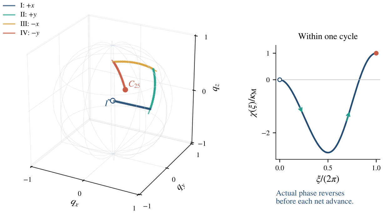
Figure 3. The four-block $SU\left(2\right)$ motion in vector quaternion coordinates $(q_x,q_y,q_z)=\mathbf{z}$. Each color traces 25 M cycles, computed from $exp\left[(j{\kappa }_{\mathrm{M}}+\chi \left(\xi \right))T\right]g_{\mathrm{start}}$; points mark completed cycles. The path includes the backward motion within each cycle, resolved by the phase curve at right. The full trajectory lies on $S^3$, whose vector-coordinate projection is the displayed ball. Periodic compensation preserves this nominal path.

Figure 3. The four-block $SU\left(2\right)$ motion in vector quaternion coordinates $(q_x,q_y,q_z)=\mathbf{z}$. Each color traces 25 M cycles, computed from $exp\left[(j{\kappa }_{\mathrm{M}}+\chi \left(\xi \right))T\right]g_{\mathrm{start}}$; points mark completed cycles. The path includes the backward motion within each cycle, resolved by the phase curve at right. The full trajectory lies on $S^3$, whose vector-coordinate projection is the displayed ball. Periodic compensation preserves this nominal path.

8. Experimental Realization and Event Statistics

The predicted recurrence concerns records left by the same selector. A response measurement determines the elementary phase; coherent matrix measurements determine its ordered product; serial records test whether that product transports the selector between readings. Measuring the response and matrices first fixes the recurrence angle before the event data are taken.

8.1. An Observation Pointer and a Two-Period Return

To read the selector, an apparatus must couple to its group coordinate. Two complex amplitudes with a common phase reference give a concrete representation. For $w={(w_1,w_2)}^T$, $w^{†}w=1$, write

$$u\left(w\right)=\left(\begin{array}{cc}{w}_1& -{\overline{w}}_2\\ w_2& {\overline{w}}_1\end{array}\right),u\left(Ww\right)=Wu\left(w\right),W\in SU\left(2\right).$$

(54)

The first column determines the whole group element. If $w_c$ is the first column of the reference c, the hemisphere coordinate is

$$h_c\left(u\right):=\frac{1}{2}\Re Tr\left(c^{†}u\right)=\Re \left(w_c^{†}w\right).$$

(55)

Mixing $Aw$ and $B{w}_c$, with real $A,B>0$, into outputs $(Aw\pm B{w}_c)/\sqrt{2}$ gives total intensities with difference $I_{+}-I_{-}=2AB{h}_c\left(u\right)$. Its sign is the hemisphere label. The common phase is essential: w and $-w$ give opposite signals, whereas a qubit ray identifies them. Coherent amplitudes with a phase reference thus give a classical analogue of the transport and readout geometry. Whether such a coordinate selects individual quantum events is a separate physical question.

The original action contains no interaction that allows the selector to displace a pointer: its base and charge equations are independent of u. Introduce a dimensionless pointer r and record coordinate ℓ on the observation axis, with conjugate momenta $p_r,p_{\ell }$, and give the apparatus the constitutive action

$$S_{\mathrm{dev}}=S+\int \left[p_r\dot{r}+p_{\ell }\dot{\ell }-{\lambda }_{\mathrm{r}}\left(t\right)p_r{h}_{c\left(t\right)}\left(u\right)-\gamma \left(t\right)p_{\ell }r\right]\mathrm{d}t.$$

(56)

Here S is Equation (8), and ${\lambda }_{\mathrm{r}},\gamma$ are prescribed rates. The first interaction moves the pointer according to the selector; the second writes its displacement into a record that survives the pointer’s return. Both coordinates belong to the observation axis. This interaction is an additional apparatus assumption, not a consequence of the event probabilities, and its physical realization remains to be established. Since c and u transform together, $h_c\left(u\right)$ and the interaction are gauge invariant.

Variation gives

$$\begin{array}{cccccccc}\hfill \dot{r}& ={\lambda }_{\mathrm{r}}{h}_c\left(u\right),\hfill & \hfill \dot{\ell }& =\gamma r,\hfill & \hfill {\dot{p}}_r& =-\gamma p_{\ell },\hfill & \hfill {\dot{p}}_{\ell }& =0,\hfill \end{array}$$

(57)

$$\begin{array}{cccccc}\hfill \dot{u}& =-{\mathcal{A}}_t^{\mathrm{su}}u,\hfill & \hfill {\dot{Q}}_{\mathrm{su}}+[{\mathcal{A}}_t^{\mathrm{su}},Q_{\mathrm{su}}]& =-{\lambda }_{\mathrm{r}}{p}_r{J}_c\left(u\right),\hfill & \hfill & J_c\left(u\right)=\frac{1}{2}(c{u}^{†}-u{c}^{†}).\hfill \end{array}$$

(58)

The same action must also be varied with respect to the original base coordinates. The direct apparatus force gives

$${\mathcal{E}}_i\left(L_0\right)=〈Q,{\mathcal{F}}_{ij}〉{\dot{b}}^j-{\lambda }_{\mathrm{r}}{p}_r{D}_i{h}_c,D_i{h}_c={\partial }_i{h}_c-〈J_c,{\mathcal{A}}_i^{\mathrm{su}}〉.$$

(59)

In the present response chart ${\mathcal{A}}_{\theta }=0$, and $c\left(t\right)$ is programmed from the nominal motion independently of the actual $\theta$, so $D_{\theta }{h}_c=0$. A disturbed readout can still alter the charge and hence the response through Equation (33). A reference with different base dependence, or another connection, also requires the direct term in Equation (59).

The identity for $J_c$ uses the traceless inner product specified with Equation (29): $\mathrm{d}{h}_c\left(\eta u\right)=〈J_c\left(u\right),\eta 〉$. At $p_r=p_{\ell }=0$, the pointer and record still move, while both momenta remain zero. Every added force on the base and charge then vanishes. This ideal classical preparation preserves the controlled response and the sector $Q_{\mathrm{su}}=0$ throughout readout.

A two-period sequence restores the $SU\left(2\right)$ selector while the response keeps moving. Put $T=2\pi /\Omega$ and continue the controlled orbit first about $+\mathbf{n}$, then about $-\mathbf{n}$. The periods give $U_{\mathbf{n}}$ and $U_{\mathbf{n}}^{-1}$. With $R\left(t\right)$ denoting their intermediate propagator, prescribe the reference along the same path:

$$R\left(0\right)=R\left(2T\right)=I,u\left(t\right)=R\left(t\right)v,c\left(t\right)=R\left(t\right)c_0,h_{c\left(t\right)}\left(u\left(t\right)\right)=h_{c_0}\left(v\right)=:h_0.$$

(60)

The reference follows the known matrix motion independently of v and of the recorded outcome. After two periods, the nominal response position, velocity and drive phase have returned; the coupling direction is restored at the end. Ideal direction switches occur at $a_t=0$. The calibration must include the return error from finite switches.

Proposition 5

(Readout with a retained selector). Prepare $r=\ell =p_r=p_{\ell }=0$. In the first period take $({\lambda }_{\mathrm{r}},\gamma )=(\Lambda /T,2/T)$, and in the second take $({\lambda }_{\mathrm{r}},\gamma )=(-\Lambda /T,0)$, with $\Lambda >0$. For the reference in Equation (60), the two-period device has the endpoint map

$$(v,0,0,0,0)⟼(v,0,\Lambda h_{c_0}\left(v\right),0,0),Y=sgn\ell .$$

(61)

Proof. 

The zero momenta preserve the original trajectory. With $h_0$ constant, direct integration gives

$$\begin{array}{ccc}& 0\le t\le T& T\le t\le 2T\\ r\left(t\right)& \Lambda h_{0}t/T& \Lambda h_0(2-t/T)\\ \ell \left(t\right)& \Lambda h_0{(t/T)}^2& \Lambda h_0\end{array}$$

(62)

The two matrix periods give $u\left(2T\right)=v$. The signs of $\ell \left(T\right)$ and $h_0$ agree, with the same fixed convention on the null boundary. This proves the map.    □

Each reading uses a fresh blank record coordinate ${\ell }_k$. Its coupling is turned off once the value is stored; previous records remain available without entering subsequent controls. The stored records are correlated with the selector, but their disconnection leaves later transport independent of their labels. Haar preservation here concerns the unconditioned selector distribution; conditioning on a record restricts it to the corresponding cell. Smooth pulses give the same endpoint structure when ${\int }_0^{2T}{\lambda }_{\mathrm{r}}\mathrm{d}t=0$ and the record gain ${\int }_0^{2T}\gamma \left(t\right){\int }_0^t{\lambda }_{\mathrm{r}}\left(s\right)\mathrm{d}s\mathrm{d}t$ is positive. The central $U\left(1\right)$ phase advances by $2{\kappa }_{\mathrm{M}}$ during the module, while its charge stays fixed. The identity return here concerns the $SU\left(2\right)$ component read by the hemispheres.

Residual pointer momenta produce the force in Equation (58) and can change the base motion. Equal and opposite pulse areas do not by themselves cancel this reaction. Its size, the reference-tracking error and the finite-switch error must all be bounded for the apparatus. A quantum reset described only by its reduced map need not realize the interaction in Equation (56).

8.2. The Response Orbit and Its Ordered Transport

The first measurement follows one free M period, without the periodic potential. The physical azimuth and the initial data in Equation (37) are chosen independently of the records. Spectroscopy determines the frequency ratio, while separately terminated runs reconstruct the observation-coordinate trajectory and its returning velocity. These measurements are needed because the holonomy depends on the whole path; an endpoint probability alone cannot determine it.

A second set of runs transfers the measured response into a coherent two-state channel governed by

$$H_{\mathrm{cal}}\left(t\right)=-\hslash a_t\mathbf{n}\left(t\right)·\sigma .$$

(63)

Its propagator satisfies $\dot{U}=i{a}_t\mathbf{n}·\sigma U$, the selector’s matrix transport equation. Coherent measurements of this channel determine the ordered product, its central sign and its control errors. The event curves then test whether this measured transport also carries the selector between records, together with the assumed cell partition and return law.

A driven three-level superconducting circuit offers a candidate for the coherent channel. The geometric operations demonstrated in such systems [9] establish the relevant control capability. Coupling those operations to the event selector through readout and return is a further requirement of the proposed realization. A reference arm or controlled-$C_{25}$ interference measurement supplies the central sign, which ordinary process tomography leaves undetermined.

The commutator is essential: a comparison of two-factor traces loses the ordering information, since $Tr\left(UV\right)=Tr\left(VU\right)$. Calibration must resolve the individual matrices and their commutator, including switching and return. At a nominal period boundary $\dot{\phi }=0$, so an ideal direction switch causes no impulsive selector rotation. The observation coordinate still moves because $\dot{\theta }\ne 0$ there. Finite switching follows this moving orbit; stopping it would require an additional force and would change the orbit. Appendix B bounds the corresponding transport error.

8.3. Readout, Return and Successive Events

The serial run retains the reference and pointer of Section 8.1 but removes the separate tomography probes. Its drive and periodic potential, Equation (41), are fixed in advance. The reference orbit is the solution of the original boundary-value problem, checked by the free one-period measurement. Each four-block transport lasts 100 elementary periods without an intermediate reading. The following two-period readout stores a record after one period and returns the pointer after the second. The periodic potential sustains the nominal response throughout this longer sequence.

The returning density operator can, for example, be described by the quantum instrument

$${\mathcal{J}}_y\left(\rho \right)=Tr\left(\rho E_y\right){\rho }_{★}.$$

(64)

This map describes one use at the reduced level. Its memoryless composition gives independent balanced records. In the present construction the fiber retains information between uses: Equation (61) stores a sign determined by the selector and returns that selector unchanged. Readout followed by the next four-block transport therefore gives

$$({\rho }_{★},u)⟼({\rho }_{★},C_{25}u),$$

(65)

with the effective entrance anchor $c_0$ unchanged. Here $u_k$ is the selector at entry to readout module k. The moving reference makes the record stored one period later equal to $Y_k=sgn{h}_{c_0}\left(u_k\right)$. For a more general apparatus, denote its complete common readout-and-return matrix by R. The next four-block transport follows that module, so

$$u_{k+1}=C_{25}R{u}_k.$$

(66)

For the nominal two-period construction, $R=I$. A nontrivial common return changes the protocol and its angle; that angle must again be determined before the event run. The product $R{C}_{25}$ has the same angle by conjugacy, but Equation (66) records the actual order of operations.

The nominal return restores $\theta =\pi /2$, its prescribed velocity, q, the hemisphere anchor, the drive phase and the $+x$ coupling. Deviations along a controlled trajectory obey Equation (45). During readout the drive clock and the potential’s reference continue to run. Pausing, advancing or compensating either changes the physical return and contributes to R. If the return depends on the outcome, the event law also changes.

Each block begins with a Haar selector at entry to its first readout module. This module acts exactly like the later ones, and no value of $Y_0$ is discarded. The assumption concerns the fiber distribution itself; a physical device must establish whether its reset or randomized controls prepare that distribution. Seven records, $Y_0$ through $Y_6$, provide the four lag comparisons. With $Y_{b,k}$ the stored sign in block b, including label errors, define

$$D_{b,N}=\mathbf{1}\{Y_{b,0}\ne Y_{b,N}\},N\in \{1,2,3,6\}.$$

(67)

The seven records require six four-block transports and seven readout modules. Consecutive records are separated by $102T$; the span from $Y_0$ to $Y_6$ is $612T$. Completing the final pointer return gives a full block duration $(6\times 100+7\times 2)T=614T$, apart from initial preparation. The predicted mismatch probabilities are unchanged and are listed together with an illustrative readout-error model:  

Lag N	$P_{\mathrm{mis}}\left(N\right)$	$C_N$	$P_{\mathrm{obs}}\left(N\right)$ at $e=0.03$
1	0.322248515	0.355502970	0.342938788
2	0.644497030	$-0.288994059$	0.627677575
3	0.966745544	$-0.933491089$	0.912416363
6	0.066508911	0.866982177	0.116967274

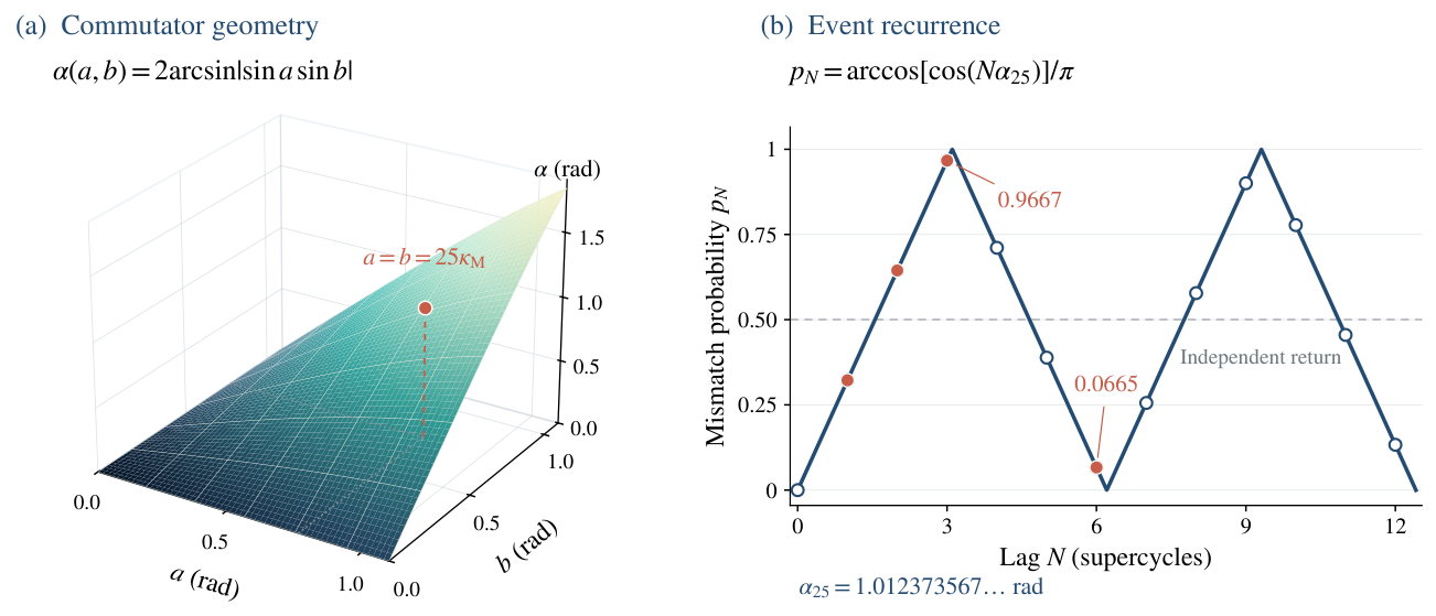
At lag three the record is almost opposite to its initial value; at lag six it is likely to have returned. The angle measured by transport fixes both features. Over two periods the continuous curve forms the M-shaped double peak in Figure 4. For this realization, the name M-event thus recalls both the retained memory and the shape of the recurrence.

The statistical comparison is made with the recorded indicators. With $p_{b,N}=Pr(D_{b,N}=1)$, define

$${\widehat{p}}_N={\displaystyle \frac{1}{B}}{\displaystyle \sum _{b=1}^B}{D}_{b,N},{\overline{p}}_N={\displaystyle \frac{1}{B}}{\displaystyle \sum _{b=1}^B}{p}_{b,N}.$$

(68)

When preparation and readout conditions are identical, ${\overline{p}}_N=P_{\mathrm{obs}}\left(N\right)$. The four comparisons within a block may be correlated; only independence between blocks is needed for the estimate below. If block probabilities differ, its center remains ${\overline{p}}_N$. For $B=2000$, four two-sided Hoeffding bounds [10] give

$$Pr\left[\underset{N\in \{1,2,3,6\}}{max}|{\widehat{p}}_N-{\overline{p}}_N|>ϵ\right]\le 8e^{-2B{ϵ}^2}.$$

(69)

A joint failure probability of $0.01$ corresponds to

$$ϵ=\sqrt{{\displaystyle \frac{log\left(800\right)}{4000}}}=0.0408797374\dots .$$

(70)

A 2000-block sample therefore gives a simultaneous statistical resolution of about $0.041$ for the four recorded probabilities. With two-period readout it requires $1.228\times {10}^6$ elementary periods, including $1.2\times {10}^6$ in the four-block transports, plus preparation and separate calibration. Its duration depends on the measured response period $T=2\pi /\Omega$; a microwave gate time from another protocol cannot supply that value. This resolution is a theoretical estimate for the proposed sample, not an achieved experimental precision.

8.4. Experimental Resolution and Control Measurements

A finite pointer error can change the label only near the hemisphere boundary. Suppose ${\ell }_k/\Lambda =h_{c_0}\left(u_k\right)+e_k$, with $|e_k|\le ϵ\le 1$, and let the error affect the record alone. A sign error then requires $\left|h\right|\le ϵ$. Integration of the $S^3$ coordinate density gives the measure of this band:

$$B\left(ϵ\right)={\displaystyle \frac{2}{\pi }}\left[arcsinϵ+ϵ\sqrt{1-{ϵ}^2}\right]\le {\displaystyle \frac{4ϵ}{\pi }}.$$

(71)

The measured and ideal mismatch indicators differ only if at least one of their labels differs. A union bound therefore yields

$$|P_{\det }\left(N\right)-P_{\mathrm{mis}}\left(N\right)|\le min\{1,2B\left(ϵ\right)\}\le {\displaystyle \frac{8ϵ}{\pi }}.$$

(72)

No independence of these label errors is required. For this source alone, $ϵ\le \pi /800$ keeps the probability error below $0.01$. Pointer offsets and reference-angle errors can be included through $ϵ=min\{1,{\delta }_{\ell }/\Lambda +2sin({\delta }_c/2)\}$ when $0\le {\delta }_c\le \pi$. If recoil changes the selector in a state-dependent way, a pointwise group-distance bound ${\Delta }_k$ from its nominal Haar trajectory contributes at most $2sin[min({\Delta }_k,\pi )/2]$ to the normalized signal error. Applying the same band bound at both endpoints remains valid even when the perturbed ensemble is no longer Haar.

An independently calibrated stochastic label model can give a more specific correction. Suppose each stored sign is flipped independently with probability e, with errors independent of the selector. The measured mismatch is then

$$P_{\mathrm{obs}}\left(N\right)=2e(1-e)+{(1-2e)}^2{P}_{\mathrm{mis}}\left(N\right).$$

(73)

This model leaves the return and later controls unchanged. Feedback from a wrong label would alter the selector transition and hence the event dynamics. Asymmetry, drift and correlated readout noise require their own measured readout law.

Transport errors are naturally measured by distance on the group. Take the actual matrices to be determined by the controls and by noise independent of the selector and previous events, and keep the hemisphere anchor fixed. Conditional on a realization of this noise, let d denote the bi-invariant $SU\left(2\right)$ geodesic distance with $d(I,W)=\alpha \left(W\right)$. If an elementary transport has distance error at most $\epsilon$ and the complete return adds at most ${\epsilon }_R$, the triangle inequality yields

$$d({\tilde{C}}_{25},C_{25})\le 100\epsilon +{\epsilon }_R=:D.$$

(74)

Repeated identical blocks, or successive blocks satisfying the same separate bound, accumulate at most $ND$ through lag N. The hemisphere law therefore gives

$$|{\tilde{P}}_N-P_N|\le min\{1,ND/\pi \}.$$

(75)

The distance bound includes errors about different axes, including noncommuting rotations. To keep the systematic probability shift below $0.01$ through lag six, it suffices to have $D\le 0.01\pi /6\simeq 0.00524$ radians. Dividing the entire allowance equally among the 100 elementary transports gives $\epsilon \le 5.24\times {10}^{-5}$ radians per transport. These are conservative requirements, not demonstrated device performance. Angle, axis and return errors must be calibrated against them before the event curve is compared with the prediction.

Several controls separate the contributions to the event curve. Parallel coupling directions make the projected commutator the identity. Omitting transport while preserving the readout schedule measures the action of readout and return. Multiplying the selector by an independent Haar element removes its correlation with earlier records and restores independent balanced events; random microwave settings establish this control only if their action on the selector is known. Ordinary apparatus memory can also be tested by interrupting accessible causal connections or changing stored classical records. The reference $P_N=1/2$ belongs to the specified independent-return protocol. General sequential quantum experiments can retain correlations, and finitely many controls cannot exclude every memory mechanism.

Varying the angle $\eta$ between the coupling directions tests Equation (50), provided that the matrices are measured in the same frame. A single recurrence curve determines only a conjugacy angle and can be reproduced by an effective circle rotation. Evidence for the non-Abelian construction must therefore come from the relation between the elementary matrices, their commutator and the family of event curves as $\eta$ varies. Reversing the commutator preserves the balanced mismatch, so this measurement determines the angle without resolving its orientation sign.

9. Conclusions

The distinction between an event probability and an individual record persists through the dynamics. Group translation preserves a Haar selector distribution, but can move a particular selector into another event cell. The Born distribution can therefore remain unchanged while the records carry a history. The M-event action determines that history through the selector motion, charge rotation and force on the physical–observation path.

In $U\left(1\right)\times SU\left(2\right)$, a central charge sustains the original M response while the matrix coupling changes direction. Four forward blocks then form a nontrivial $SU\left(2\right)$ commutator without reversing the response trajectory. The original free orbit and its phase are also preserved by the periodic compensation potential. What changes is the motion around the orbit: exponentially growing deviations become harmonic.

Reading this motion requires an interaction with the selector. In the stated ideal classical preparation, the observation-pointer action writes the hemisphere coordinate into a record, restores the reusable pointer and returns the $SU\left(2\right)$ selector after two periods. The stored record is then decoupled from later control. The measure of a band around the hemisphere boundary bounds the effect of finite pointer resolution without assuming independent label errors.

For the faithful fixed-axis coupling, balanced hemispheres and common return $R=I$, the original phase fixes ${\alpha }_{25}=1.01237356667423\dots$. The record is almost opposite to its initial sign after three supercycles and almost restored after six, while either outcome retains probability $1/2$ at every reading. These predictions concern the specified preparation, transport and return. Their physical interpretation requires the measured response and matrix operations to act on the same retained selector; agreement with one event sequence would not identify its microscopic carrier.

The resulting test concerns what survives a return of the observable conditions. The endpoint probabilities are restored, yet the order of the intervening operations can remain in the relation between records. For the realization studied here, that relation is a recurrence curve with an angle determined before the event data are taken.

9.1. Outlook

The pointer action fixes a relation among the selector, the pointer and the stored record, while leaving the response medium open. A microscopic interpretation must identify $r,\ell$, their coupling to $h_c\left(u\right)$ and their residual conjugate momenta. Phase-referenced coherent amplitudes furnish a classical analogue. A quantum-event realization requires the further identification of the retained coordinate with the selector of individual records. The theory thus distinguishes a realizable transport geometry from the still open physical interpretation of its event coordinate.

The sector of zero traceless charge isolates ordering while preserving the original M orbit. Away from it, the charge projection in Equation (33) changes the response, and the response changes subsequent transport. Both phase and matrix must then be calculated on the same coupled trajectory; the original constant cannot be inserted in advance. A continuation to nonzero-charge periodic motion and finite-momentum readout should retain this action together with Equation (59). The two-period forward and reverse coupling returns the selector under the zero-charge preparation used here; it is not a general return proof for a charged trajectory.

Larger compact groups allow event partitions with more than two outcomes. For a fixed endpoint partition, an independent Haar initial selector and a given transport W, the mismatch probability has the general form

$$P_{\mathrm{mis}}\left(W\right)=1-\sum _y\mu \left(C_y\cap W^{-1}{C}_y\right).$$

(76)

The intersection contains precisely those initial points that give label y at both readings. For $SU\left(2\right)$ hemispheres, its volume reduces to one angle. For groups such as $SU\left(3\right)$ and more than two labels, the probability involves more general cell intersections. Their geometry poses a natural question: which partitions admit both a physical readout and a tractable relation between transport and the correlations of several event types?

The present construction gives a probability pairing, fiber comparison, driven response and persistent record, without exhausting the observation space. Coupling directions, the readout anchor and the pulse rates remain prescribed apparatus choices. Their recurrence curves are compared here; no optimum over all observation controls is asserted. A further choice of readout should first fix its gain, duration and realizable control bounds, then calculate errors in its actual records from the same action.

Even within the present $SU\left(2\right)$ realization, axis angle and block length m give a family of predictions once the response and coupling have been calibrated. The angle formula and error bounds describe the corresponding changes in signal, duration and control accuracy. Their joint dependence tests more of the theory than agreement at a single numerical fingerprint.

References

- X. Meng. The Natural Dual-Axis Structure of Observation: Categorical Foundations and Consequences for Quantum Theory, Preprints 2026. [CrossRef]
- Meng, X. Deterministic Quantum Events on a Dual-Axis State Bundle: A Falsifiable Recurrence Test of Single-Event Continuity, Preprints supplied revised manuscript and Supplemental Material. 2026. [CrossRef]
- Berry, M. V. Quantal phase factors accompanying adiabatic changes. Proc. R. Soc. Lond. A 1984, 392, 45–57. [Google Scholar] [CrossRef]
- Wilczek, F.; Zee, A. Appearance of gauge structure in simple dynamical systems. Phys. Rev. Lett. 1984, 52, 2111–2114. [Google Scholar] [CrossRef]
- Haar, A. Der Massbegriff in der Theorie der kontinuierlichen Gruppen. Ann. Math.>, Second Ser. 1933, 34(2), 147–169. [Google Scholar] [CrossRef]
- Hall, B. C. Lie Groups, Lie Algebras, and Representations: An Elementary Introduction . In Graduate Texts in Mathematics, 2nd ed.; Springer: Cham, 2015; Vol. 222. [Google Scholar] [CrossRef]
- Magnus, W. On the exponential solution of differential equations for a linear operator. Commun. Pure Appl. Math. 1954, 7(4), 649–673. [Google Scholar] [CrossRef]
- Floquet, G. Sur les équations différentielles linéaires à coefficients périodiques. Ann. Sci. De l’École Norm. Supérieure, Second Ser. 1883, 12, 47–88. [Google Scholar] [CrossRef]
- Abdumalikov, A. A., Jr.; Fink, J. M.; Juliusson, K.; Pechal, M.; Berger, S.; Wallraff, A.; Filipp, S. Experimental realization of non-Abelian non-adiabatic geometric gates. Nature 2013, 496, 482–485. [Google Scholar] [CrossRef] [PubMed]
- Hoeffding, W. Probability inequalities for sums of bounded random variables. J. Am. Stat. Assoc. 1963, 58(301), 13–30. [Google Scholar] [CrossRef]
Figure 4.
Noncommuting transport geometry and event recurrence. (a) The conjugacy angle for orthogonal control axes; the red point marks . (b) The same angle determines two full periods of the M-shaped recurrence when the selector is retained. Circles denote the formula at integer supercycles, with the four prescribed lags highlighted in red; the solid curve is its continuous extension. The dashed line denotes independent balanced preparations.
Disclaimer/Publisher’s Note: The statements, opinions and data contained in all publications are solely those of the individual author(s) and contributor(s) and not of MDPI and/or the editor(s). MDPI and/or the editor(s) disclaim responsibility for any injury to people or property resulting from any ideas, methods, instructions or products referred to in the content. |
© 2026 by the authors. Licensee MDPI, Basel, Switzerland. This article is an open access article distributed under the terms and conditions of the Creative Commons Attribution (CC BY) license (http://creativecommons.org/licenses/by/4.0/).
Copyright: This open access article is published under a Creative Commons CC BY 4.0 license, which permit the free download, distribution, and reuse, provided that the author and preprint are cited in any reuse.