

Submitted:
18 September 2026
Posted:
20 September 2026
You are already at the latest version
Abstract
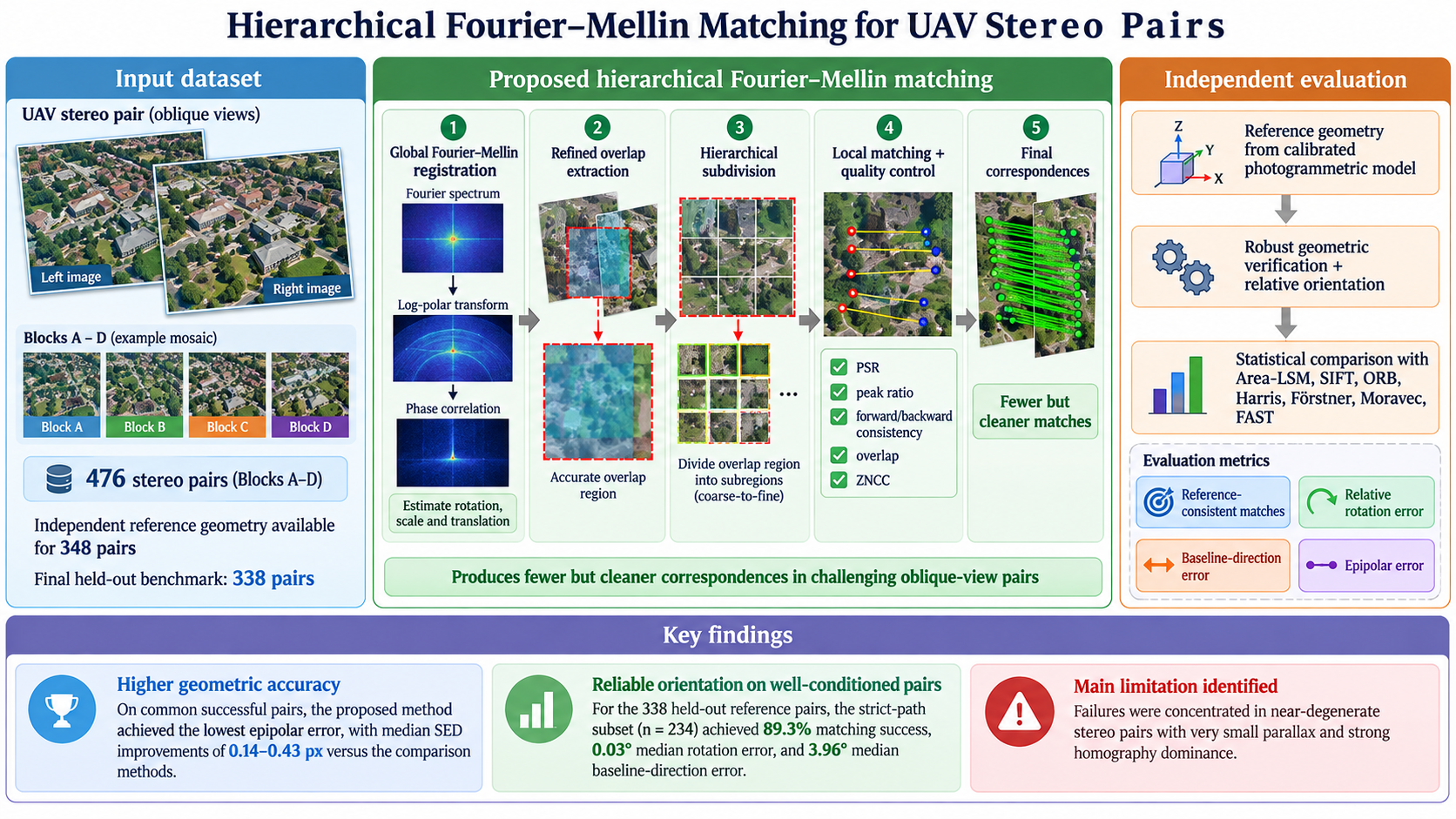
Accurate image correspondences are essential for geometric inference in vision-based UAV sensing because camera pose, 3D reconstruction, and spatial measurement depend on the geometric validity of matched points rather than on match count alone. This study develops a hierarchical Fourier–Mellin/phase-correlation framework for sequential RGB imagery acquired by a UAV camera sensor. Global similarity registration is followed by recursive local refinement with spectral, forward–backward, overlap, and radiometric acceptance criteria. Performance was assessed on 338 held-out stereo pairs using independently bundle-adjusted camera geometry as an external reference and a common relative-orientation pipeline for all methods. The proposed method achieved 63.91% matching success and 60.06% reference-valid success, compared with 89.05% and 27.81%, respectively, for Area-LSM. For successfully oriented pairs, median relative-rotation and baseline-direction errors were 0.0322° and 3.7987°, respectively. On common successfully oriented pairs, the proposed approach yielded lower errors than Area-LSM and ORB, whereas SIFT, Harris, Förstner, Moravec, and FAST generally retained higher success rates and lower errors. Baseline-direction accuracy was strongly dependent on parallax and homography dominance. These results support independent sensor-geometry validation and geometry-aware hybrid matching for UAV vision-based sensing.
Keywords:
UAV vision-based sensing
; camera sensor
; image matching
; Fourier–Mellin transform
; phase correlation
; relative orientation
; geometric validation
; 3D sensing
1. Introduction
Automatic correspondence establishment between aerial images is a key stage in vision-based sensing and the photogrammetric processing of data acquired by unmanned aerial vehicles (UAVs). Coordinates of corresponding points are used to determine the relative image geometry, estimate relative orientation parameters, perform spatial ray intersection, and subsequently reconstruct the three-dimensional structure of the scene [1,2,3]. Consequently, errors introduced during correspondence search directly affect the robustness and accuracy of subsequent geometric computations.
In vision/camera-based sensing, image matching and relative orientation are closely related but distinct tasks. Image matching establishes the image coordinates of the same objects or ground points in two images, whereas relative orientation determines the relative camera rotation and the direction of the spatial baseline from previously established correspondences. This distinction is fundamental when evaluating a sensing pipeline: a large number of matches does not, by itself, guarantee correct two-view geometry, whereas a smaller set of geometrically reliable correspondences may be sufficient for robust pose recovery and subsequent 3D inference.
A classical class of photogrammetric matching techniques comprises area-based methods, which directly compare the radiometric structure of local image patches. These include correlation-based approaches and Least-Squares Matching (LSM) for correspondence refinement [1,4]. Their principal advantage is the direct use of radiometric information and the potential to achieve subpixel accuracy when a sufficiently accurate initial approximation is available. However, area-based methods are sensitive to relative image rotation, scale differences, perspective and local geometric distortions, and illumination changes. These limitations become particularly important for oblique UAV imagery and stereo pairs with varying spatial baselines.
Another widely used class comprises feature-based matching methods. Moravec, Harris, Förstner, and FAST detectors, together with SIFT and ORB, provide sparse sets of localized image features that can be matched across images [5,6,7,8,9,10]. SIFT provides invariance to changes in local image scale and orientation [7], whereas ORB combines FAST with the binary BRIEF descriptor and is designed to reduce the computational cost of matching [10]. Harris, Förstner, Moravec, and FAST differ in their feature-detection principles and localization accuracy; consequently, their performance may depend strongly on scene texture and stereo-pair geometry.
An alternative approach exploits the spectral properties of images. Phase correlation estimates the relative translational displacement between two images directly in the frequency domain without requiring an initial displacement vector [4,11,12]. By transforming Fourier-magnitude spectra into log-polar coordinates, relative rotation and scale change can likewise be converted into a translational estimation problem, which forms the basis of the Fourier–Mellin approach [11,13]. Frequency-domain methods are therefore attractive for coarse automatic registration of images affected by unknown translations, rotations, and scale differences.
Fourier-based methods have been investigated extensively in remote sensing and photogrammetry [11,12,13,14,15,16,17]. Previous studies have shown that phase correlation can provide robust translation estimates and can be applied to stereo matching, while the Fourier–Mellin transform extends the registration model to include scale changes and rotation. However, the classical Fourier–Mellin transform describes a similarity transformation and therefore cannot directly represent the general projective deformation between two perspective aerial images. With a non-negligible baseline, non-parallel image planes, and a spatially heterogeneous scene, a single global transformation becomes only an approximation to the actual two-view geometry.
One way to address this limitation in a camera-based sensing pipeline is to adopt a hierarchical strategy in which global frequency-domain registration is used only to obtain an initial approximation, after which the overlap region is recursively divided into smaller patches. Within local regions, perspective deformation can be approximated more accurately, allowing similarity-transform estimates to generate a spatially distributed set of correspondences. Such a strategy, however, requires reliable acceptance criteria for local solutions because an erroneous phase-correlation registration in a single patch may generate correspondences that are internally consistent with an incorrect model but do not represent the actual two-view sensor geometry.
From a sensor-validation perspective, independent assessment of correspondence quality is therefore particularly important. Metrics computed with respect to a fundamental matrix estimated from the same correspondences characterize internal self-consistency, but do not by themselves demonstrate agreement with the independently determined acquisition geometry. Objective comparison requires an external geometric reference that is not involved in the operation of the evaluated matching algorithm. In this study, camera parameters obtained from an independent bundle adjustment in Pix4Dmapper were used for this purpose. They are treated not as absolute ground truth, but as a common camera-geometry reference for comparing the outputs of different correspondence-establishment methods.
For camera-based 3D sensing, an additional challenge arises in the estimation of relative translation. Relative orientation of two images allows the relative rotation and baseline direction to be recovered, but the absolute scale of the two-view solution cannot be determined from image correspondences alone. Moreover, baseline-direction accuracy depends strongly on the geometric conditioning of the stereo pair. Under low-parallax conditions and strong homography dominance, displacement of the projection center is weakly observable; consequently, the translation direction may be unstable even when the relative-rotation error remains small. Evaluation of a vision-based sensing pipeline should therefore consider not only aggregate error statistics but also the geometric conditions of individual stereo pairs.
The objective of this study is to develop and experimentally evaluate a hierarchical method for automatic correspondence establishment in UAV camera imagery based on a combination of the Fourier–Mellin transform and phase correlation, and to determine its applicability for vision-based geometric sensing relative to area-based LSM and classical feature-based methods. The methodological contributions are threefold. First, we formulate a deterministic hierarchical Fourier–Mellin/phase-correlation framework in which global registration is progressively refined within local overlap regions and a correspondence is retained only after the current local solution satisfies predefined spectral, geometric, and radiometric quality criteria. Second, we introduce an independent camera-geometry validation framework based on bundle-adjusted UAV camera orientations, explicitly separating correspondence-generation success from external geometric validity. Third, we benchmark the proposed approach against Area-LSM, SIFT, ORB, Harris, Förstner, Moravec, and FAST on a predefined held-out dataset using an identical relative-orientation pipeline for all methods, and quantify how stereo-pair conditioning affects relative-rotation and baseline-direction accuracy.
2. Materials and Methods
2.1. Study Area, UAV Platform, Camera Sensor, and Image Acquisition
The study was conducted in Kyiv, Ukraine. The aerial survey area is predominantly flat and includes tree and grass vegetation, vehicular and pedestrian roads, open spaces, and buildings of varying heights. This combination provides both well-textured and comparatively homogeneous image regions, allowing the matching algorithms to be evaluated under different scene-structure conditions.
The sensing platform consisted of a DJI Mavic 4 Pro Fly More Combo quadcopter operated with a DJI RC 2 controller. The primary Hasselblad camera served as the imaging sensor and incorporated a 4/3-inch CMOS image sensor. RGB images were recorded at a resolution of 6144 × 4096 pixels. The camera interior orientation parameters refined during subsequent calibration and bundle adjustment are described separately in Section 2.2.
The acquisition produced a sequence of 485 images, from which 484 consecutive image pairs could potentially be formed. However, not all consecutive pairs were used in the comparative experiment. Pairs corresponding to transitions between distinct platform-motion and camera-orientation regimes were excluded during formation of the experimental blocks. The final experimental dataset comprised 476 stereo pairs; their formation and allocation to Blocks A–D are described in Section 2.3.
Camera/gimbal orientation telemetry stored in the metadata of each image was used to characterize the acquisition conditions, specifically the yaw, pitch, and roll angles. Across the analyzed sequence, pitch ranged from 0.0° to −46.1°, with a mean of −30.35° and a median of −30.0°. Yaw ranged from −176.1° to 157.3°, while roll was 0.0° in all 485 metadata records.
The variation in pitch and yaw along the image sequence is shown in Figure 1. The experimental blocks are displayed not as single intervals between their minimum and maximum image numbers, but as the actual continuous sequence segments used in the analysis. This distinction is important because some blocks comprised several spatially separated parts of the acquisition. In particular, Block A consisted of two segments, Blocks B and C also comprised multiple segments, whereas Block D occupied one continuous part of the sequence. This representation makes it possible to relate changes in camera orientation directly to the acquisition segments actually used for method comparison.
Because yaw is represented cyclically within the range from −180° to +180°, the plotted line was interrupted between adjacent samples whenever the absolute difference between the displayed values exceeded 180°. This break removes an artificial line between equivalent branches of the angular representation and does not indicate missing telemetry data.
Thus, the formation of Blocks A–D extends the analysis beyond a simple comparison of methods on a single image set and enables evaluation of matching performance under different stereo-pair geometric conditions.
2.2. Camera Calibration, Preliminary Photogrammetric Processing, and Pix4D Reference Model
Ground control and check-point coordinates were measured using a Meridian M20L GNSS receiver operating in RTK mode. In total, coordinates were determined for 45 ground points within the study area. Measurements were performed in EPSG:9864 — UCS-2000 / LCS-80 Kyiv city; the geodetic reference system was UCS-2000 with the Ukraine 2000 datum and the Krassowsky 1940 ellipsoid. Point elevations were determined in the normal-height system. The study area and ground-point distribution are shown in Figure 2.
Following the initial image analysis and preliminary photogrammetric solution, 23 of the 45 surveyed ground points were excluded from further processing. The main reasons were the absence of a reliable image of the point in the aerial photographs, visibility in only a small number of frames, insufficiently unambiguous visual identification, or an adverse effect on the stability of the photogrammetric adjustment. The final ground-control configuration comprised 22 points: 6 ground control points (GCPs) and 16 check points (CPs).
Preliminary photogrammetric processing of all 485 images was performed in Pix4Dmapper 4.10.1. The project was georeferenced using six GCPs with known three-dimensional coordinates. According to the Pix4Dmapper Quality Report generated during image processing, 6 GCPs (6 3D) were used for georeferencing, with a mean RMS error of 0.018 m. The sixteen CPs were not used as constraints in the adjustment and served for independent assessment of the spatial accuracy of the photogrammetric solution. After initial georeferencing, image exterior orientation parameters and camera parameters were jointly refined by bundle adjustment.
A perspective camera model was used to represent the imaging sensor. After optimization, 360 of the 485 images were calibrated, corresponding to 74.23% of the complete dataset. The mean reprojection error of the final solution was 0.224 pixels, and the relative difference between the initial and optimized camera interior orientation parameters was 3.95%.
The optimized camera focal length was:
and the principal-point coordinates were:
Accordingly, the camera intrinsic matrix used in the subsequent geometric computations was:
The optimized radial distortion coefficients were , , and , whereas the tangential distortion coefficients were and . The initial and optimized interior orientation parameters are summarized in Table 1.
Full-resolution images were used during the initial Pix4Dmapper solution. Automatic keypoint extraction was performed without a predefined fixed number of features. The Aerial Grid or Corridor strategy was used for the initial image matching.
For all subsequent experimental matching algorithms, images to which the optical-distortion correction model had already been applied were used. Therefore, the coefficients , , , , and were retained to document the camera calibration model but were not applied again to point coordinates during correspondence analysis. This avoided double distortion correction and ensured that all evaluated methods operated in a common pixel coordinate system.
For independent geometric validation of the matching results, projection centers and rotation matrices of the calibrated cameras were extracted from the final Pix4D project. Exterior orientation parameters were available for both cameras in 348 of the 476 experimental stereo pairs. These 348 pairs therefore formed the subset for which an independent Pix4D reference geometry could be constructed. This geometry was used not as absolute ground truth, but as a common external photogrammetric reference model obtained independently of the matching algorithms under evaluation.
2.3. Stereo-Pair Formation and Experimental Blocks
A sequence of 485 images theoretically yields 484 consecutive image pairs. However, not all consecutive pairs represented homogeneous acquisition segments. Some pairs lay at boundaries between segments with different camera orientations and UAV-motion characteristics. To exclude these transitions from the comparative experiment, eight consecutive pairs were removed, yielding a final dataset of 484 − 8 = 476 stereo pairs.
The selected pairs were assigned to four experimental Blocks A–D. Block A contained 10 pairs, Block B 124 pairs, Block C 31 pairs, and Block D 311 pairs, for a total of 476 stereo pairs.
This common set of 476 pairs was used as the initial dataset for comparison of all correspondence-establishment algorithms.
The blocks were defined according to the camera-orientation regime and the position of the corresponding segments within the acquisition sequence. Block A comprised segments with a horizontally oriented camera, for which the telemetry-derived pitch angle was approximately 0°. Block B was characterized by a nearly constant camera tilt with pitch of approximately −32.2°. Block C comprised transitional and more strongly tilted segments, with pitch varying from approximately −46.1° to −29.5°. Block D represented the main oblique-survey segment and contained 311 pairs with an almost constant pitch of approximately −30.0°.
Two characteristics were used to describe the geometry of each pair: the telemetry-derived inter-frame spatial displacement and the angle between the camera optical-axis directions. Spatial displacement was determined from image positions recorded in the flight metadata by transforming WGS84 geodetic coordinates to the Earth-Centered, Earth-Fixed (ECEF) system and computing the Euclidean distance between the positions of two consecutive exposures. Because the accuracy and resolution of the source GNSS metadata are limited, a calculated zero displacement for individual pairs indicates identical recorded coordinates at the available precision and is not interpreted as strictly zero physical UAV motion.
The angle between the optical axes was determined from the telemetry-derived yaw and pitch angles. For image i, the unit viewing-direction vector was defined as:
where φ and θ denote the yaw and pitch angles, respectively. Under this convention, corresponds to a horizontal optical-axis direction, whereas corresponds to the downward direction.
The angle between the viewing directions of two images was computed from their scalar product:
Before this model was used in the final analysis, its convention was independently validated on 348 stereo pairs for which both cameras had been calibrated in Pix4Dmapper. Relative to angles obtained directly from the Pix4D rotation matrices, the telemetry-based model yielded a mean absolute error of 0.078°, a median absolute error of 0.021°, an RMSE of 0.413°, and a Pearson correlation coefficient of . This convention was therefore used to characterize all 476 experimental pairs.
The geometric characteristics of the blocks are summarized in Table 2. The distribution of the telemetry-derived baseline and optical-axis angle is shown in Figure 3. The full range is presented in Figure 3a, whereas Figure 3b provides an enlarged view of the region containing small inter-frame displacements and small angles, where a substantial proportion of the consecutive pairs is concentrated.
Table 2 summarizes the main characteristics of the 476 stereo pairs included in the comparative experiment. The baseline was calculated from onboard GNSS metadata and is used as a descriptive measure of inter-frame displacement; zero values may occur because of the limited coordinate resolution in the metadata. The optical-axis angle was calculated from yaw and pitch using the telemetry model independently validated against Pix4Dmapper camera orientations.
2.4. Methods for Establishing Point Correspondences
The comparative experiment was designed to assess the ability of different algorithms to automatically establish corresponding feature points in sequential aerial images acquired from a moving platform. In photogrammetry, corresponding (homologous) points are points in the left and right images of a stereo pair that represent the same object-space point. The evaluated approaches belonged to several methodological classes: area-based matching, least-squares matching, local-feature detectors and descriptors, and methods based on phase correlation and the Fourier–Mellin transform, including the enhanced method proposed in this study.
The common objective of all methods was to generate a set of point correspondences. All compared methods used the same preprocessed images as input, thereby excluding differences in distortion correction or image-geometry modification as factors affecting the matching results. The methods were evaluated on the same set of stereo pairs and using a common subsequent geometric-validation procedure.
2.4.1. Area-Based Matching
Area-based methods operate by directly comparing image-intensity values in local patches of two images. In the classical photogrammetric formulation, a local window is centered on the point to be measured, and the corresponding position in the second image is determined by maximizing a similarity measure or minimizing a dissimilarity measure. Because this approach directly exploits the radiometric information in the images, it can achieve high local matching accuracy, but it is sensitive to scale changes, relative rotation, image tilt, and illumination differences. Consequently, area-based methods become less robust as the geometric differences between the two images increase.
In this study, Area-Based Matching was implemented as a two-stage procedure. In the first stage, sparse local features were used to establish coarse geometric guidance and to estimate an initial fundamental matrix . The resulting geometric information constrained the search region for the corresponding point in the second image.
The maximum of the normalized cross-correlation (NCC) function was then sought within the local search region. An epipolar constraint was used to reject candidates that deviated substantially from the predicted epipolar line. This both reduced the probability of false correlation maxima and restricted the computational search domain.
The resulting coarse position was used as the initial approximation for subsequent local least-squares refinement.
2.4.2. Affine Least-Squares Matching
To improve local matching accuracy after the coarse NCC estimate, full affine Least-Squares Matching (LSM) was applied. This differs fundamentally from simple subpixel interpolation of the correlation maximum because LSM directly estimates the local geometric deformation of the image patch [18].
A six-parameter model was used for points within the local window:
where denote the refined coordinates of the corresponding point, and the coefficients describe the local linear transformation of the window, including scaling, rotation, stretching, and shear deformation.
Refinement was performed iteratively using the Gauss–Newton method. Image gradients were used to construct the Jacobian, while intensities in the transformed window were evaluated by bilinear interpolation. The parameter vector was updated until the convergence criterion was satisfied or the maximum number of iterations was reached.
Additional constraints were imposed to ensure physical plausibility of the solution. A solution was rejected if the refined point was displaced excessively from the initial approximation or if the affine matrix became degenerate. These constraints reduced the influence of locally homogeneous regions and unstable solutions. The final fundamental matrix was estimated from the refined correspondences using RANSAC.
2.4.3. Feature-Based Matching
The second group comprised algorithms based on local image features (feature-based matching). Unlike area-based methods, which directly compare the intensity structure of predefined image patches, feature-based approaches first detect a set of localized keypoints and then describe and match them between the two images. Six feature-based methods were evaluated against the proposed Fourier–Mellin method: SIFT, ORB, Harris, Förstner, Moravec, and FAST [5,6,7,8,9,10]. All methods were applied to the same full-resolution Pix4D images after distortion correction, as described in Section 2.2.
SIFT and ORB were used as complete detector–descriptor pipelines. For SIFT, the native OpenCV implementation was used to perform both keypoint detection and SIFT-descriptor computation. The maximum number of retained keypoints per image was limited to 4000. SIFT produces a real-valued local descriptor based on the spatial distribution of image-intensity gradients, providing robustness to changes in image scale and orientation [7].
ORB was likewise used through its native OpenCV implementation as a combined detector and binary descriptor. The maximum number of keypoints was 4000; the pyramid scale factor was 1.2, eight pyramid levels were used, the local patch size was 31 pixels, and the FAST threshold was 20. Keypoints were ranked using the Harris score. Unlike SIFT, ORB produces binary descriptors, allowing descriptor distances to be computed efficiently using the Hamming metric [10].
In this experiment, Harris, Förstner, Moravec, and FAST were used primarily as keypoint detectors. Harris identifies local regions with pronounced intensity variation in two independent directions using the second-moment matrix of image gradients [6]. The Förstner operator exploits local gradient structure and is designed for precise localization of point features, which is particularly relevant to photogrammetric applications [8]. The Moravec detector evaluates intensity changes produced by shifting a local window in several directions and identifies points exhibiting strong two-dimensional variation. FAST identifies corner points by examining pixel intensities on a circle around a candidate center and is designed for high computational efficiency [5,8,9].
For Harris, Förstner, and Moravec, the number of detected points was limited to 4000, the minimum distance between local response maxima was 3 pixels, and the relative response threshold was 0.01. FAST used an intensity threshold of 20 with non-maximum suppression enabled; after ranking by response magnitude, no more than 4000 points were retained.
Because Harris, Förstner, Moravec, and FAST do not inherently produce descriptors, a common normalized intensity descriptor was used to ensure a uniform matching procedure. Before descriptor construction, the detected point coordinates were refined to subpixel precision using cornerSubPix with a 5 × 5-pixel window. The termination criteria were a maximum of 30 iterations and an accuracy of 0.01 pixels.
For each refined point, a square 31 × 31-pixel patch was extracted from the image. Let denote the vector of pixel intensities in this patch. The normalized descriptor was defined as , where is the mean patch intensity, is the standard deviation of the intensities, and denotes conversion of the two-dimensional patch into a one-dimensional vector. This normalization reduces sensitivity to additive and multiplicative intensity differences between images and enables a common matching procedure for all four detector-only methods.
Descriptor correspondences were established by brute-force nearest-neighbour matching. For each descriptor in the first image, the two nearest candidates in the second image were identified. The Hamming metric was used for ORB, whereas Euclidean distance was used for SIFT and for the normalized intensity descriptors associated with Harris, Förstner, Moravec, and FAST.
To suppress ambiguous matches, a ratio test was applied. A match was accepted if , where and are the distances to the first and second nearest neighbours, respectively. For SIFT, was used, whereas for ORB, Harris, Förstner, Moravec, and FAST, was used.
The correspondences obtained at this stage were treated as tentative matches. To remove geometrically inconsistent correspondences, a fundamental matrix was estimated from them using RANSAC. At least eight correspondences were required to initiate the estimation. The RANSAC threshold was set to 1.5 pixels, the confidence level to 0.999, and the maximum number of iterations to 10,000. Correspondences classified as RANSAC inliers constituted the final point-correspondence set for the respective feature-based method.
Accordingly, all six methods followed the same processing sequence:
- detection;
- description;
- nearest-neighbour matching;
- ratio test;
- RANSAC geometric filtering.
The descriptor-generation stage nevertheless differed among the methods: SIFT and ORB used their native descriptors, whereas Harris, Förstner, Moravec, and FAST used the same normalized 31 × 31-pixel intensity descriptor. This design allowed the effect of the different keypoint-detection strategies to be compared under an otherwise identical downstream description, matching, and geometric-filtering procedure.
No separate LSM refinement was applied to the feature-based correspondences. An additional cornerSubPix refinement was also not applied to SIFT or ORB, because their keypoint coordinates and descriptors were generated directly by the native implementations of the respective methods.
It is also important to distinguish the internal geometric filtering of feature-based correspondences from their subsequent independent quality assessment. The RANSAC procedure described above was part of each baseline method's own matching pipeline and was used to reject gross outliers. It was not regarded as independent confirmation of the correctness of the recovered geometry. Independent validation of the final correspondences against the external Pix4D reference geometry was performed separately, as described in Section 2.5.
Table 3 summarizes the principal implementation parameters of the feature-based methods used in the comparative experiment. SIFT and ORB used their native descriptors, whereas Harris, Förstner, Moravec, and FAST used the common normalized intensity descriptor.
2.4.4. Phase Correlation Method
Phase correlation (PC) is used to estimate the relative translational displacement between two images directly in the frequency domain and does not require an a priori displacement vector [4,11,12]. In the proposed algorithm, phase correlation serves as a basic computational operation at two stages: first, to estimate shifts in the log-polar domain of the Fourier–Mellin transform, and second, to determine the residual spatial translation after scale and rotation compensation. The complete Fourier–Mellin procedure is described in Section 2.4.5.
Let the two images be represented by the functions and , and let their two-dimensional Fourier transforms be denoted by and , respectively, where are the spatial frequencies. If the images differ only by a translation vector , then, for , the Fourier shift theorem gives the following relationship between their spectra:
Thus, translation changes the phase component of the spectrum without changing its amplitude. The relative image displacement can therefore be estimated from the normalized cross-power spectrum:
where denotes complex conjugation and is a small positive constant that prevents numerical instability when the magnitude of the cross-spectrum approaches zero. In this study, was used.
After applying the inverse Fourier transform:
a correlation surface is obtained with a localized maximum. The position of this maximum determines the translational correction between the images. In the implemented convention, define the correction that maps the second image into the coordinate system of the first.
The fast Fourier transform algorithm was used for both the forward and inverse transforms. At the spatial phase-correlation stage, two-dimensional forward and inverse FFTs were applied because only the translational component is estimated at this stage. The full complex two-dimensional spectrum, with the zero spatial frequency shifted to the center, is used separately for the Fourier–Mellin estimation of scale and rotation and is described in Section 2.4.5.
Image Periodization Preprocessing
An important feature of the implementation is the preliminary reduction of discontinuities at image boundaries. The discrete Fourier transform assumes periodic continuation of the analyzed signal: the first row or column is implicitly assumed to follow the last one. In real images, values on opposite boundaries generally differ, generating artificial high-frequency components that can reduce the localization of the correlation peak.
To mitigate this effect, the periodization procedure developed by the authors was retained in the present implementation. First, a linear component caused by differences between opposite image boundaries was removed.
If is the original image of size , the vertical correction can be written as:
An analogous correction was then applied in the horizontal direction:
After periodization, the image mean was subtracted:
This spatial phase-correlation stage should be distinguished from the separate spectral stage of the Fourier–Mellin procedure. In spatial PC, the periodization described above is the primary means of reducing boundary effects, whereas construction of the Fourier–Mellin spectrum additionally employs a Hann window.
Correlation-Surface Smoothing
After the inverse FFT, the correlation surface was smoothed with a two-dimensional Gaussian filter with a standard deviation of px. This smoothing suppresses local noise fluctuations and stabilizes localization of the principal correlation peak.
Correlation-Peak Quality Assessment
Two measures were used to assess the prominence and uniqueness of the peak: the peak-to-sidelobe ratio (PSR) and the ratio of the primary peak to the second-highest peak.
When computing PSR, a square region with a radius of five pixels around the principal maximum was excluded, with the periodicity of the correlation surface taken into account. The mean and standard deviation were computed over the remaining sidelobe region.
PSR was defined as:
where is the value of the principal correlation peak.
The ratio of the primary peak to the second peak was computed as
where is the maximum value of the correlation surface outside the excluded neighborhood of the principal peak.
For spatial phase correlation, the following acceptance conditions were used:
If either condition was not satisfied, the translation estimate was rejected as insufficiently pronounced or ambiguous.
These conditions characterize the shape of the correlation peak itself. They form part of, but do not constitute the entire, quality-control procedure for Fourier–Mellin registration. Additional checks include forward/backward displacement consistency, the fraction of actual image overlap, and the radiometric similarity of the aligned images; these are described in Section 2.4.7.
Subpixel Refinement
To improve localization accuracy, the coordinates of the discrete maximum were refined to subpixel precision. A periodic 3 × 3-pixel neighborhood was used. For positive values of the correlation surface, its logarithm was approximated by a quadratic function:
The vertex of the fitted surface was determined from the condition:
In expanded form, the subpixel correction coordinates can be obtained from the system
It was additionally verified that the matrix of second derivatives corresponded to a local maximum, i.e., that both of its eigenvalues were negative.
To prevent an unstable displacement of the fitted vertex beyond the local neighborhood, the subpixel corrections were constrained as follows:
If the approximation was degenerate or the resulting quadratic surface did not correspond to a maximum, the original integer coordinates of the correlation peak were retained.
Correlation-Peak Width
In addition to the peak coordinates, its full width at half maximum (FWHM) was determined. Along the horizontal and vertical profiles through the principal peak, the first positions at which the correlation function decreased to were identified. After determining the widths in both directions, the following measure was used: . In the present implementation, FWHM was not interpreted as an independent absolute error of the corresponding-point position. Instead, it was used as a measure of correlation-peak localization and as one of the criteria controlling and terminating further hierarchical image subdivision.
Accordingly, the basic spatial phase-correlation procedure can be summarized as follows:
- ;
- periodization;
- mean removal;
- FFT;
- normalized cross-power spectrum;
- IFFT;
- Gaussian smoothing;
- peak detection;
- ;
- subpixel refinement;
This procedure is a fundamental computational component of the proposed algorithm, but it does not by itself constitute the complete method. In Fourier–Mellin registration, phase correlation is first applied in log-polar space to generate scale and rotation hypotheses and is then applied in the spatial domain to estimate the residual translation. Construction of the Fourier–Mellin spectrum additionally uses a full two-dimensional FFT, spectrum centering, a Hann window, and logarithmic compression of the dynamic range. These operations are described in Section 2.4.5.
2.4.5. Fourier–Mellin-Based Matching
The Fourier–Mellin transform extends phase-correlation-based registration from translation-only estimation to the case in which the images also differ in rotation and scale [11,13,19]. The central idea is to use the magnitude of the two-dimensional Fourier spectrum and represent it in log-polar coordinates. Because spatial translation primarily changes the spectral phase according to Equation (1), the spectral magnitude can first be used to estimate scale and rotation largely independently of translation, after which the remaining spatial displacement is determined by phase correlation according to Equations (2)–(3).
Let images and be related by a similarity transformation comprising a scale factor , a rotation through angle , and a translation . In general form, this transformation can be written as:
where the two-dimensional rotation matrix is
According to the properties of the Fourier transform, a spatial translation changes the phase component of the spectrum, whereas relative rotation and scaling appear as a geometric transformation of its magnitude. For the model in Equation (13), the spectral magnitudes can be expressed as
where denotes the frequency-domain coordinates. The factor changes the spectral amplitude but does not affect the location of its structures, which is used to estimate the geometric-transformation parameters.
Before spectrum construction, each analyzed fragment was processed using the periodization procedure described by Equations (4)–(6), after which its mean value was subtracted. A two-dimensional Hann window, defined as the product of one-dimensional windows along the two coordinates, was then applied:
Where
Here, and are the width and height of the analyzed fragment, respectively. The window further reduces the contribution of boundary regions to the spectrum and mitigates the effect of residual non-periodicity.
A full complex two-dimensional Fourier spectrum was computed for the resulting image. The spectral samples were then shifted so that the zero spatial-frequency component was located at the center of the spectral plane. This centering is required for the subsequent transformation to polar coordinates, whose origin must coincide with the zero spatial frequency.
The magnitude of the centered spectrum was used. To compress the dynamic range and reduce the dominance of the strongest low-frequency components, the following logarithmic transformation was applied:
where is the centered two-dimensional Fourier spectrum. The function , rather than the complex spectrum itself, was then transformed to log-polar coordinates. Thus, the implemented processing sequence comprises periodization, mean removal, a two-dimensional Hann window, the full centered spectrum, and the transformation .
The transformation from Cartesian frequency-domain coordinates to polar coordinates was performed using:
The radial coordinate was then replaced by its logarithmic form . Accordingly, the log-polar representation of the spectrum can be written as:
The advantage of this representation is that rotation and scaling of the original image become translational shifts along the two coordinates and . Taking the model in Equation (13) into account, the relationship between the log-polar spectral representations of the two images can be written, up to the adopted transformation direction, as
Consequently, estimation of scale and rotation is reduced to the estimation of a two-dimensional translational shift, for which the phase-correlation procedure described in Section 2.4.4 is used [13,19].
In the implemented method, the logarithmic radial coordinate was formed over the range from to , where are the coordinates of the center of the spectral image. Excluding the immediate vicinity of the zero frequency reduces the influence of the dominant central component, whereas the maximum-radius constraint ensures that the circular analysis region lies entirely within the spectral image. The angular coordinate covered the full range .
For sufficiently large fragments, up to 256 samples were used along the logarithmic radial coordinate and up to 512 samples along the angular coordinate. For smaller fragments, the number of samples was automatically limited by their actual spatial dimensions. Thus, rows of the log-polar image corresponded to coordinate , whereas columns corresponded to angle .
Let phase correlation between the two log-polar representations yield a displacement along the angular coordinate and along the logarithmic radial coordinate. The angular sampling step is then , and the logarithmic radial sampling step is , where and are the numbers of angular and radial samples, respectively.
The initial rotation-angle estimate is given by , whereas the initial estimate of the logarithm of scale is . Therefore:
Thus, the displacement along the angular coordinate is used to estimate rotation, whereas the displacement along the logarithmic radial coordinate is used to estimate scale. This coordinate correspondence was used in the final implementation of the algorithm.
Phase correlation in log-polar space followed the same general procedure as the spatial phase correlation described by Equations (2)–(3). The quality of the spectral correlation peak was assessed using and , defined by Equations (7) and (8). Because phase correlation at this stage was performed in log-polar space and was used only to generate candidate scale and rotation hypotheses, the following thresholds were applied:
These thresholds are hereafter referred to as the spectral criteria of the log-polar stage.
At this stage, the correlation surface was smoothed with a Gaussian filter with a standard deviation of px. If the conditions in Equation (23) were not satisfied, the spectral scale-and-rotation estimate was rejected and the corresponding fragment was not passed to subsequent registration.
Unique recovery of the transformation from the spectral magnitude alone is limited by known symmetries of the Fourier–Mellin representation. In particular, the magnitude spectrum of a real-valued image is centrosymmetric, producing a 180° rotational ambiguity. In addition, the sign of the angular displacement and the direction of the scale transformation depend on which image is treated as the reference and which is transformed to it.
Therefore, instead of accepting a single pair , a set of alternative hypotheses was generated:
After angle normalization and removal of duplicate variants, no more than eight unique hypotheses were retained. The admissible global scale range was constrained by .
The generation of the symmetric hypotheses , , and the variants differing by 180° directly reflects the scale-and-rotation estimation procedure used in the implementation.
For each hypothesis from the set (24), the second image was rotated and scaled about its center using cubic interpolation. After compensation for scale and rotation, the remaining difference between the images was treated as predominantly translational and was estimated by spatial phase correlation according to Equations (2)–(3).
Thus, each spectral hypothesis yielded a transformation mapping coordinates from the second image into the coordinate system of the first:
where is the center of the analyzed image, and are the tested scale and rotation parameters, and is the translational correction obtained by phase correlation.
When determining , the spatial correlation peak was required to satisfy the and criteria defined by Equations (7) and (8), using the thresholds
i.e., the same conditions introduced in Section 2.4.4. In addition, translation was estimated in both the forward and reverse directions. The complete criteria for forward/reverse consistency, minimum overlap, radiometric similarity, and final selection among admissible Fourier–Mellin hypotheses are described separately in Section 2.4.7.
To limit the computational cost of Fourier–Mellin registration, large fragments were resampled to a common reduced resolution before spectral analysis while preserving their aspect ratio. If the largest fragment dimension exceeded 1536 pixels, the fragment was downsampled so that its maximum side was px.
Both images in a pair were reduced by the same factor. After successful registration, the estimated translational shifts and spatial characteristics of the correlation peak were converted back to pixel units of the original fragment. Fourier–Mellin registration was not performed for fragments whose minimum dimension was less than 128 pixels. Thus, large fragments were analyzed in a common reduced coordinate system, after which the accepted spatial parameters were transformed back to the original resolution.
Accordingly, one Fourier–Mellin registration cycle can be summarized as follows:
- ;
- periodization and mean removal;
- Hann window;
- centered Fourier magnitude;
- ;
- log-polar representation;
- phase correlation;
- hypotheses;
- rotation and scale compensation;
- spatial phase correlation;
The resulting similarity transformation was used as either a global or a local estimate of the relative geometry of the corresponding fragment. However, a single similarity transformation cannot fully represent the perspective differences between two aerial images when a non-zero spatial baseline and a non-planar scene are present. The proposed method therefore embeds Fourier–Mellin registration within a hierarchical scheme in which the overlap region is progressively subdivided into smaller fragments. This procedure is described in Section 2.4.6.
2.4.6. Proposed Hierarchical Fourier–Mellin Matching
The Fourier–Mellin registration described in Section 2.4.5 estimates a similarity transformation comprising relative scaling, rotation, and translation. For two perspective aerial images, a single global similarity transformation is only an approximation to the actual two-view geometry because the spatial baseline, camera tilt, and three-dimensional scene structure produce spatially varying image deformations. Therefore, in the proposed method, global Fourier–Mellin registration is used to obtain an initial geometric approximation, after which the region of actual overlap is processed recursively at the local level.
The proposed procedure comprises two consecutive global-registration stages followed by hierarchical local registration. At each stage, the Fourier–Mellin transform is used to estimate scale and rotation, whereas the residual translation is determined by spatial phase correlation. Mapping coordinates from the second image into the coordinate system of the first follows the model defined by Equation (25).
At the first global stage, Fourier–Mellin registration was applied to the entire image pair. The scale , relative rotation , and translational correction were estimated, and these parameters defined the global transformation:
which compensated for the dominant relative scale, rotation, and displacement between the images.
After applying , the actual overlap between the first image and the transformed second image was determined. The largest admissible rectangular region fully contained within their common overlap was retained for subsequent processing. If no sufficiently large overlap region existed, processing of the corresponding stereo pair was terminated.
The first global transformation was treated as an initial approximation and was further refined. The second image was first transformed using , and the common overlap region was extracted from both images. Fourier–Mellin registration was then repeated for these approximately aligned fragments. At this stage, a residual transformation was estimated, and the refined global transformation was obtained by sequential composition of the two estimates: .
Because most of the original relative transformation had already been compensated at the second global stage, the estimated residual transformation was expected to remain close to the identity transformation. The admissible residual scale, rotation, and translation, together with the remaining Fourier–Mellin acceptance conditions, are specified in Section 2.4.7.
After the second global refinement, the actual image overlap was recomputed with respect to transformation . This refined overlap region served as the initial domain for hierarchical local processing.
At the initial hierarchical level, the entire rectangle of refined overlap was treated as a single current fragment. The corresponding region in the second image was determined using the accumulated parent transformation. This region was prewarped into the coordinate system of the current fragment of the first image, after which a new complete Fourier–Mellin registration was performed for the current fragment pair according to the procedure in Section 2.4.5.
Thus, local geometry was not inherited directly from the global solution. The global or parent transformation was used only to obtain a preliminarily aligned region of the second image; the residual local transformation still had to be independently confirmed by the image content of the current fragment.
Let be the accumulated transformation of the parent level and the residual similarity transformation estimated for the current fragment at level . The refined transformation of the current fragment was then defined as .
After each successful local refinement, the actual overlap of the current fragment was recomputed using the updated transformation . Further subdivision was therefore performed only within the part of the fragment for which geometrically admissible overlap was preserved after local registration.
If successful registration of the current fragment did not satisfy a stopping condition, the overlap region was divided into smaller parts. At the first subdivision level, a 2 × 3 grid was used, i.e., the current region was divided into two rows and three columns. At subsequent levels, each successfully registered fragment was subdivided according to a 2 × 2 scheme.
This non-uniform initial subdivision provided a denser spatial distribution of local regions immediately after global alignment, whereas subsequent four-way recursive subdivision enabled progressive refinement of the local geometry.
The minimum nominal fragment size eligible for further subdivision was 256 pixels along each side. Fragments with either width or height below 128 pixels were not passed to Fourier–Mellin registration. The maximum hierarchy depth was limited to seven levels.
One stopping criterion was the FWHM of the correlation peak, defined in Section 2.4.4. For a current fragment of width and height , its mean linear dimension was computed as
The stopping threshold was defined as one-half of this dimension:
If the condition was satisfied after successful local registration, no further spatial subdivision of that fragment was performed. This rule limited attempts at additional localization when the correlation peak remained broad relative to the size of the analyzed fragment.
Recursive subdivision was also terminated when the current fragment width or height was no greater than 256 pixels, when the next subdivision would have produced child regions smaller than the admissible size, when there was insufficient overlap to form child fragments, or when the maximum hierarchy depth had been reached.
A key requirement of the proposed scheme was that a corresponding point could be generated only after successful Fourier–Mellin registration of the current fragment. If local registration failed to satisfy the specified quality criteria, the corresponding branch of the hierarchy was terminated, and coordinates predicted solely by the parent transformation were not accepted as a confirmed correspondence.
In other words, an unsuccessful local registration produced no corresponding point. This rule prevents artificial inflation of the correspondence count through inheritance of the global or parent transformation in regions where the local image structure does not support the estimated geometry.
If the current fragment was successfully registered and reached one of the stopping conditions, it became terminal. The corresponding point in the first image was defined as the center of the terminal fragment:
Because the accumulated transformation maps coordinates from the second image into the first-image coordinate system in accordance with the transformation direction adopted in Equation (25), the corresponding point in the second image was obtained using the inverse transformation:
Thus, the corresponding-point coordinate in the second image was determined not simply from the center of an analogous rectangle, but from the complete accumulated transformation, including global registration, global residual refinement, and all successful local refinements along the corresponding hierarchical branch.
After all branches had been processed, the resulting correspondences were merged into a single set. To suppress spatially duplicated results, a minimum separation of 12 pixels was imposed between corresponding points in the second image. If several results occurred within this distance, the correspondence with the higher quality score was retained
where characterizes the radiometric similarity of the fragments after complete geometric alignment, whereas characterizes the prominence of the spatial phase-correlation peak. The definition of is given by Equation (7); the acceptance criteria for , , forward/reverse consistency, and minimum overlap are specified in Section 2.4.7.
Accordingly, the proposed scheme can be summarized by the following sequence:
- global Fourier–Mellin registration;
- global residual refinement;
- refined overlap;
- local Fourier–Mellin registration;
- 2 × 3 initial subdivision;
- 2 × 2 recursive subdivision;
- independent validation of each current fragment;
- terminal-fragment correspondences;
- duplicate suppression.
Unlike applying a single similarity transformation to an entire stereo pair, this organization represents the spatially non-uniform relative image deformation through a set of locally refined transformations. Global Fourier–Mellin registration provides the initial geometric approximation, whereas each final corresponding point is generated only from a successfully validated registration of the associated local fragment.
2.4.7. Acceptance and Quality-Control Criteria
The reliability of Fourier–Mellin registration was assessed using a combination of independent spectral, geometric, and radiometric criteria rather than a single indicator. This multistage verification is necessary because a pronounced maximum on the correlation surface does not, by itself, guarantee that the estimated transformation is correct. A false spectral hypothesis may produce a locally distinct correlation peak while failing to provide consistent forward and reverse alignment or sufficient radiometric agreement after the complete geometric transformation.
The first level of control was applied in log-polar space. The spectral correlation peak was assessed using and , defined by Equations (7) and (8), with the thresholds specified in Equation (23):
This stage was used only to generate admissible hypotheses . The final decision was made after scale and rotation compensation followed by analysis in the spatial domain.
For each admissible spectral hypothesis, the translational displacement was estimated by phase correlation in both the forward and reverse directions. In forward registration, the second image was mapped into the first-image coordinate system and the displacement was estimated, whereas reverse registration yielded .
Both spatial phase-correlation estimates were required to satisfy independently the criteria in Equation (26):
Thus, a strongly pronounced correlation peak was required in both the forward and reverse registration directions.
Because mutually consistent transformations should yield forward and reverse translation vectors with opposite directions, the forward/backward consistency error was defined as:
For the primary strict acceptance mode, the following condition was used: .
This threshold was defined in the pixel coordinate system of the image actually used for Fourier–Mellin analysis. If the original fragment was downsampled before spectral processing as described in Section 2.4.5, was evaluated in that reduced coordinate system. After a decision was made, translation parameters and other spatial characteristics were converted back to pixels of the original fragment. In the implementation, the forward/backward error was computed as the norm of the sum of the forward and reverse displacement vectors, with a strict threshold of 1.5 pixels in the analysis-resolution image.
After the complete similarity transformation defined by Equation (25) had been applied, the actual geometric overlap of the images was also checked. Let be the number of pixels in the second image that map inside the first image after transformation, and let and denote the width and height of the analyzed first-image fragment. The fraction of actual overlap was defined as:
A candidate was required to satisfy . In addition, radiometric verification was performed only when at least valid jointly observed pixels were available. This overlap fraction and minimum valid-pixel count were used when evaluating the fully aligned images.
Radiometric agreement after complete alignment was assessed using zero-mean normalized cross-correlation (ZNCC). For the set of valid overlapping pixels Ω, the measure was computed as
where is the second image after complete alignment with the first, and the mean values are computed only over Ω. Standard candidate acceptance required .
ZNCC was computed only from valid transformed pixels and excluded regions artificially filled during geometric image transformation.
Accordingly, after satisfying the spectral criterion in Equation (23) and the forward and reverse spatial phase-correlation criterion in Equation (26), a standard Fourier–Mellin candidate was additionally required to satisfy:
These criteria were applied to both global and local Fourier–Mellin registration.
The current hierarchical level was also taken into account. At the first global stage, the broad admissible scale range defined in Section 2.4.5 was used. After the first global alignment, the second global solution represented only a residual correction; consequently, narrower constraints were imposed:
where is the diagonal length of the fragment used during global refinement.
For hierarchical local registration, the constraints were still more restrictive because each current child fragment had already been preliminarily aligned using the accumulated parent transformation. The residual local deformation was therefore required to lie within the range
where is the diagonal length of the current local fragment. The implementation used scale ranges of 0.85–1.15 with a 15° rotation limit for the second global refinement and 0.90–1.10 with a 12° rotation limit for the local residual transformation; the admissible translation magnitudes were 0.50 and 0.35 times the fragment diagonal, respectively.
For the two global stages, a restricted alternative acceptance mode with a slightly larger forward/backward consistency error was additionally available. It was considered only when none of the hypotheses satisfied the standard condition in Equation (31). The spectral criteria in Equation (23), the forward and reverse spatial criteria in Equation (26), the minimum overlap fraction, and the minimum number of jointly observed pixels remained unchanged. An alternative global candidate could be accepted only under the following conditions:
Increasing the ZNCC threshold from 0.15 to 0.50 in this case compensated for the slightly relaxed forward/backward-consistency requirement. This alternative mode was not used at local hierarchical levels. If at least one candidate satisfied the standard condition in Equation (31), it had unconditional priority over any candidate accepted under Equation (34), irrespective of its ZNCC value. This rule was applied at both global stages.
If several admissible hypotheses belonged to the same acceptance class, the final candidate was selected sequentially according to four criteria. The primary criterion was the maximum ZNCC value; if results were equal or close, preference was given to the larger minimum PSR across the forward and reverse phase correlations, then to the larger minimum , and finally to the smaller forward/backward error. This lexicographic sequence can be written as:
The candidate with the maximum value of this ordered criterion set was selected. In the implementation, ZNCC is therefore the primary selection criterion, followed by PSR, peak ratio, and the smaller forward/backward error.
At the local level, a corresponding point was never inherited from the parent transformation after unsuccessful registration. Consequently, failure to satisfy any mandatory criterion for the current local fragment terminated that branch of the hierarchy without generating a corresponding point, as described in Section 2.4.6.
After hierarchical search and spatial duplicate suppression, a stereo pair was considered to provide a sufficient correspondence set for subsequent two-view geometric processing if it contained at least eight final corresponding points. This value is consistent with the minimum number of correspondences required for subsequent fundamental-matrix estimation.
In summary, the quality-control system of the proposed method combines four independent levels of verification: reliability of the spectral scale-and-rotation estimate, prominence of the spatial correlation peak, geometric consistency of forward and reverse registration, and independent verification of the fully aligned fragments using overlap and ZNCC. A final corresponding point is therefore generated not merely from a phase-correlation maximum, but only after sequential confirmation of the spectral, spatial, and radiometric consistency of the estimated transformation.
2.5. Independent Camera-Geometry Validation
After completion of the method-specific matching procedure, the quality of the resulting correspondences was evaluated against an independent photogrammetric reference model. This separation is important because a small epipolar error relative to a fundamental matrix estimated from the same correspondences primarily reflects the internal consistency of that point set and does not, by itself, confirm agreement with the actual relative camera geometry. Therefore, camera parameters obtained from an independent bundle adjustment in Pix4Dmapper were used as the primary external geometric reference.
As described in Section 2.2, exterior-orientation parameters were available for 360 of the 485 images. Both cameras had calibrated exterior-orientation parameters for 348 of the 476 experimental stereo pairs. These pairs constituted the complete set on which independent geometric validation could be performed. The Pix4D model was used only after correspondence generation and did not participate in image pre-orientation, candidate formation, or geometry tuning for any of the evaluated methods.
For the standard methods—Area-LSM, SIFT, ORB, Harris, Förstner, Moravec, and FAST—the final correspondence set retained by each method after its own geometric filtering was passed to the independent validation stage. For the proposed Fourier–Mellin method, the correspondences validated by the hierarchical procedure and the criteria in Section 2.4.7 were used. Thus, the independent validation compared the final output of each matching pipeline without altering its method-specific correspondence-generation procedure.
The Pix4D camera parameters were represented by the model:
where denotes the coordinates of a 3D point, is the projection center of camera i in the object-space coordinate system, is the rotation matrix from object space to the corresponding camera coordinate system, and denotes the point coordinates in the camera coordinate system.
For two images, the relative rotation from the first camera coordinate system to the second and the corresponding translation vector were defined as:
Consequently, the coordinates of the same 3D point in the two camera coordinate systems are related by:
This convention for relative rotation and translation was used to construct the reference geometry and follows directly from the Pix4D exterior-orientation model.
For each stereo pair, the corresponding reference essential matrix was constructed as:
where is the skew-symmetric cross-product matrix associated with .
Using the camera intrinsic matrices and , the reference fundamental matrix was computed as:
The computational implementation first constructs and then ; normalization of is used only to obtain a numerically stable representation because the fundamental matrix is defined up to a nonzero scale factor.
Under the convention adopted in the computations, the corresponding homogeneous image coordinates were:
For an ideal correspondence, they satisfy the independent epipolar constraint:
This orientation of the fundamental-matrix equation was kept fixed throughout the independent validation; under the opposite photogrammetric convention, the corresponding fundamental matrix differs by transposition [20].
For each detected correspondence, the distance from the point in the first image to the corresponding reference epipolar line and the analogous distance in the second image were computed. The reference epipolar lines were defined as:
Using the notation the directional distances were:
The primary error measure for an individual correspondence was the mean of the two directional distances:
This symmetric pixel-domain error was evaluated with respect to the fixed Pix4D fundamental matrix rather than a fundamental matrix recovered from the correspondence set being tested. The implemented measure therefore corresponds to the mean distance to the epipolar lines in the two images.
The primary pre-specified threshold for independent geometric consistency was:
For each method and stereo pair, the number of correspondences satisfying the condition (44) was determined as
where is the number of final correspondences generated by the method, and is the indicator function.
The fraction of correspondences consistent with the independent reference geometry was defined as:
The 1.5-pixel threshold was used as the primary criterion in all inter-method comparisons. For diagnostic purposes, the fractions of correspondences satisfying thresholds of 0.5, 1.0, 2.0, and 3.0 pixels were also calculated; however, these supplementary levels did not replace the primary criterion in Equation (44). In the final comparative protocol, the number of correspondences consistent with the Pix4D reference geometry at 1.5 pixels was used as the principal measure of independent geometric validity.
A stereo pair was considered geometrically validated against the independent Pix4D model if at least eight correspondences satisfied the condition in Equation (44):
Two levels of success were therefore distinguished. Matching success indicated that a method generated at least eight final correspondences irrespective of external geometric validation, whereas reference-valid success required at least eight correspondences that agreed with the independent Pix4D reference geometry at the 1.5-pixel threshold. This distinction separates an algorithm's ability to generate a sufficient number of correspondences from the ability of those correspondences to reproduce externally defined two-view geometry.
Metrics computed relative to a fundamental matrix estimated from the same correspondences could be used as supplementary measures of internal consistency, but they were not treated as the primary criterion of geometric accuracy. This distinction is important because low SED or Sampson residuals relative to a self-estimated fundamental matrix may occur even when the recovered matrix differs substantially from the independent photogrammetric geometry. Accordingly, the principal measures at this stage were , and the fraction of stereo pairs satisfying Equation (47). The need for such independent validation became evident during diagnostics of self-estimated epipolar residuals: a low error relative to a self-estimated did not guarantee a small error relative to the Pix4D reference .
The availability of Pix4D reference geometry was a prerequisite for independent validation, but its numerical characteristics were not used to select stereo-pair difficulty, algorithm thresholds, or matching parameters. Of the 348 pairs for which reference geometry was available, a small subset was used during method development and was excluded from the final independent comparison. The formation of the development and held-out subsets is described in detail in Section 2.7.
After validation of the correspondences against , their ability to recover relative orientation was assessed using a common computational pipeline for all methods. Estimation of relative rotation and the spatial baseline direction is described in Section 2.6.
2.6. Relative Orientation Estimation
Following the independent assessment of correspondence consistency described in Section 2.5, the relative-orientation parameters were estimated for each method. The purpose of this stage was to recover the relative camera rotation and the direction of the spatial baseline from the correspondences produced by each matching algorithm. The same downstream computational procedure was applied to all compared methods so that differences in relative-orientation performance would primarily reflect the quality of the input correspondence sets rather than differences between pose-recovery algorithms [2,20].
It should be emphasized that the Pix4D reference geometry introduced in Section 2.5 was not used to estimate relative orientation. In particular, the condition (44) was not applied to preselect points before pose estimation. The reference model was used only after an independent solution had been obtained, in order to compute relative-rotation and baseline-direction errors. The pose-estimation procedure therefore remained independent of the reference solution.
For the standard methods, their final correspondence sets after method-specific internal geometric filtering were passed to this stage. For the proposed method, the final correspondences generated by the hierarchical procedure in Section 2.4.6 and Section 2.4.7 were used. To ensure identical downstream processing, all correspondence sets were additionally subjected to a common robust fundamental-matrix estimation stage using MAGSAC++ within the Universal Sample Consensus (USAC) framework [21]. The same parameters were used for all methods: a geometric residual threshold of 1.5 pixels, a confidence probability of 0.999, and a maximum of 10,000 iterations. If fewer than eight robustly consistent correspondences remained, relative orientation was not estimated for that stereo pair.
Estimation of the Fundamental Matrix
After the common robust selection stage, the fundamental matrix was re-estimated from the remaining correspondences using the normalized eight-point algorithm. This re-estimation ensured that, after robust inlier selection, the same deterministic two-view geometry estimator was applied to all methods.
Let the homogeneous coordinates of the i-th correspondence in the first and second images be:
The same fundamental-matrix convention as in Section 2.5 was used:
Before linear estimation, the point coordinates in each image were normalized using Hartley transformations. For each point set, the centroid was translated to the origin and the scale was chosen so that the mean distance of the points from the origin was . If and denote the corresponding normalization transformations, then
For the normalized coordinates
each correspondence contributed one row to the linear-system matrix
The vector of fundamental-matrix elements was obtained as the solution of the homogeneous system
using the singular value decomposition of . A rank-2 constraint was then imposed on the resulting normalized fundamental matrix: for the singular value decomposition
the smallest singular value was set to zero:
After denormalization, the fundamental matrix was computed as
Thus, coordinate normalization, linear eight-point estimation, explicit enforcement of the rank-2 constraint, and subsequent denormalization were consistently used in the common fundamental-matrix estimation procedure.
Essential Matrix and Relative Pose
Because the camera intrinsic parameters were known from the photogrammetric adjustment, the fundamental matrix was converted to an essential matrix:
where , are the intrinsic calibration matrices of the first and second cameras, respectively. For the imagery used in this study, they corresponded to the calibrated camera model described in Section 2.2.
Ideally, an essential matrix has two equal nonzero singular values and one zero singular value. Therefore, for
the value was computed, after which the following matrix was used:
Thus, the singular-value constraint of the form (σ, σ, 0) was explicitly imposed when converting from to .
The essential matrix defines relative pose with a four-fold ambiguity. Given
two candidate rotation matrices were formed as
and the translation direction was defined by the third column of :
Accordingly, four possible pose solutions were considered:
The final solution was selected using the cheirality condition. For each candidate, the corresponding viewing rays were linearly triangulated using the projection matrices
For a physically admissible solution, the reconstructed 3D point must lie in front of both cameras:
Among the four candidates, the solution with the largest number of points satisfying Equation (61) was selected. In addition, the fraction of correctly triangulated points with positive depth in both cameras was required to be at least
In the implemented algorithm, all four combinations were tested, and the solution with the largest number of positive-depth points was preferred. The minimum admissible positive-depth fraction was fixed at 0.50.
Photogrammetric Baseline Direction
The translation obtained from essential-matrix decomposition is not itself the photogrammetric baseline vector between the projection centers. Under the convention adopted in Section 2.5 and Section 2.6, the relative geometry is written as:
If is the baseline vector from the first projection center to the second, expressed in the first-camera coordinate system, then
Consequently, , and the normalized direction of the photogrammetric baseline was defined as
This relationship is fundamental: the translation direction recovered from essential-matrix decomposition and the photogrammetric baseline direction are expressed in different coordinate systems. In the implementation, the baseline direction was therefore computed as . The same relationship was used to construct the Pix4D reference geometry: .
It should also be noted that two-view geometry estimated from corresponding image coordinates does not determine the absolute translation scale. Accordingly, this study evaluated only the direction of the recovered baseline, not its magnitude. Relative orientation was therefore characterized by three relative-rotation parameters and two independent parameters describing the baseline direction, i.e., five independent geometric degrees of freedom [2,20].
Accuracy Relative to the Pix4D Reference
For each method, the recovered relative rotation was compared with the reference rotation derived from the Pix4D exterior orientations according to Equation (37). The residual rotation matrix was defined as
The angular relative-rotation error was computed from the trace of this matrix:
Before evaluating the arccosine, its argument was numerically clipped to the interval [−1, 1]. This metric represents the minimum rotation angle required to align the estimated orientation with the reference orientation.
For the Pix4D reference model, the baseline direction in the first-camera coordinate system was obtained directly from the projection centers:
The baseline-direction error was defined as the angle between the estimated and reference unit vectors:
The quantities , were used as the primary relative-orientation accuracy metrics. The implementation computed the rotation error from the residual rotation matrix defined in Equation (65), whereas the baseline-direction error was computed as the angle between and .
For each stereo pair, the relative-orientation solution was considered successful if the common robust stage retained at least eight correspondences, the normalized eight-point fundamental-matrix estimation and essential-matrix construction were completed successfully, and the cheirality-selected solution satisfied the criterion (62). For successful solutions, the values , were retained.
Accordingly, the common relative-orientation pipeline was:
- final correspondences of each method;
- common robust geometric verification;
- normalized eight-point ;
- ;
- essential-matrix constraint;
- four candidates;
- cheirality;
- ;
- , .
Applying the same procedure after matching ensured direct comparability of the results: the same two-view geometry recovery algorithm was used for all methods, while the Pix4D reference geometry was used only for subsequent independent error assessment and not for constructing the estimated solution.
2.7. Development and Held-Out Evaluation Protocol
To avoid optimistic bias from tuning method parameters and then evaluating performance on the same data, stereo pairs with available independent Pix4D reference geometry were partitioned in advance into development and held-out subsets. Of the 348 experimental pairs for which Pix4D exterior-orientation parameters were available for both images, 10 pairs from Block D were assigned to the development subset. These pairs were used only during development and finalization of the spectral implementation, hierarchical scheme, and acceptance criteria described in Section 2.4.5, Section 2.4.6 and Section 2.4.7. They were excluded from the subsequent final quantitative comparison of the methods.
After the algorithm was fixed, the remaining 348 − 10 = 338 stereo pairs formed the held-out subset. It comprised 55 pairs from Block B, 25 from Block C, and 258 from Block D. Block A was absent from the held-out subset because none of its experimental pairs had Pix4D exterior orientations simultaneously available for both images. The final partition therefore contained 10 development pairs and 338 held-out pairs, with the held-out distribution across Blocks A/B/C/D equal to 0/55/25/258, respectively.
Reference epipolar errors, parallax, homography inlier ratios, relative-orientation errors, and other numerical characteristics of the Pix4D reference geometry were not used when forming the held-out subset. Pix4D information was used solely to determine whether an independent reference orientation existed for a given stereo pair. The 10 pairs used previously for development were then removed from the set of reference pairs. Thus, neither the difficulty nor the expected quality of individual stereo pairs was a criterion for inclusion in the final evaluation.
All final performance measures for the proposed method—including matching success, independent geometric consistency, and relative-orientation accuracy—were computed only on the 338 held-out pairs. The same 338 stereo pairs were used in the final comparison with Area-LSM, SIFT, ORB, Harris, Förstner, Moravec, and FAST, ensuring an identical evaluation domain for all methods. The development and held-out subsets had no overlap in the final comparative analysis.
After the held-out results had been obtained, the parameters of the proposed algorithm were not modified further. This development/held-out separation was used so that the final performance measures reflected the ability of the fixed method to process stereo pairs that had not been used during its development.
2.8. Pair Geometry Conditioning
The accuracy of the recovered spatial baseline direction depends not only on correspondence quality but also on the geometric conditioning of the stereo pair itself. In particular, small parallax reduces the observability of the translational component, while geometry that is well described by a single homography is characteristic of approximately planar or weak-parallax configurations. Therefore, in addition to the primary comparison on all 338 held-out stereo pairs, a separate analysis was conducted to examine how relative-orientation errors depend on stereo-pair geometry.
This analysis was an additional stratification rather than an inclusion criterion for the main dataset. The thresholds defining the geometric regimes were fixed before the final analysis of the held-out subset and were not used to modify parameters of either the proposed method or any baseline algorithm. Pairs for which geometric characteristics could not be determined reliably remained in the main comparison of all 338 pairs but were excluded from the stratified analysis.
To ensure that the geometric classification was not determined directly by the results of the proposed method or Area-LSM, an independent anchor-correspondence set was constructed from the results of six feature-based methods: SIFT, ORB, Harris, Förstner, Moravec, and FAST. The proposed Fourier–Mellin method and Area-LSM were excluded from this construction. For each feature-based method, only correspondences consistent with the independent Pix4D reference geometry at the primary threshold of px established in Equation (44) were retained.
To prevent a method producing particularly large numbers of points from dominating the anchor set, no more than 1000 correspondences were retained from each feature-based method. After merging, spatially close duplicates were removed, and the resulting set was limited to 5000 correspondences per stereo pair. At least eight such anchor correspondences were required to compute the geometric characteristics.
For the i-th correspondence, the homogeneous image coordinates were converted to unit camera rays:
Because the relative rotation maps directions from the first-camera coordinate system to the second, the ray from the second image was transformed into the first-camera coordinate system as:
The parallax angle of a correspondence was defined as
Before numerical evaluation of the arccosine, the dot-product value was constrained to [−1, 1] to prevent undefined values caused by finite-precision rounding.
This computation follows the procedure actually used: normalized rays were constructed from the intrinsic calibration matrices, after which the second-camera ray was transformed into the first-camera coordinate system using the transpose of the reference rotation matrix.
The median of the parallax angles was used as a robust stereo-pair characteristic:
The second characteristic quantified homography dominance. A planar projective homography was robustly estimated from the same anchor correspondences, after which the fraction of correspondences consistent with that homography was computed as:
where is the number of homography inliers and is the total number of anchor correspondences used. Robust homography estimation employed a 2.0-pixel threshold, a confidence probability of 0.999, and a maximum of 10,000 iterations.
Based on and , the stereo pairs were assigned to three geometric regimes:
These thresholds were fixed from preliminary diagnostics before analysis of the final held-out dataset.
The near-degenerate category therefore represents the joint presence of very small parallax and strong agreement with a single homography. In contrast, the well-conditioned category requires appreciable parallax and comparatively weak homography dominance. All remaining pairs for which both characteristics were available were assigned to the intermediate category. If a reliable independent anchor-correspondence set was unavailable or either geometric characteristic could not be computed, the pair was classified as unclassified.
The resulting classes were used only to interpret the relative-orientation errors , defined by Equations (66) and (68). They were not used for correspondence generation, pose estimation, or formation of the primary held-out benchmark.
2.9. Statistical Analysis
Statistical comparisons were performed on the fixed held-out subset of 338 stereo pairs, which was identical for all eight evaluated methods. The proposed Fourier–Mellin method was compared pairwise with each of the seven baseline methods: Area-LSM, SIFT, ORB, Harris, Förstner, Moravec, and FAST. The paired design allowed the methods to be compared on the same stereo pairs and therefore avoided confounding from differences in sample composition.
Three binary endpoints were considered: matching success, defined as the presence of at least eight final correspondences; reference-valid success, defined as the presence of at least eight correspondences satisfying the independent condition (44) as specified by Equation (47); and relative-orientation success, defined as successful completion of the common procedure in Section 2.6, including the cheirality criterion (62).
For each binary endpoint, the difference between the proposed method and the corresponding baseline was characterized by the difference in success proportions
Statistical significance of the binary differences was assessed using a two-sided exact McNemar test, which uses only discordant pairs, i.e., stereo pairs successfully processed by only one of the two compared methods. A 95% confidence interval for Δp was additionally obtained using a paired bootstrap with 20,000 resamples of stereo pairs with replacement. Thus, the final statistical protocol used the exact McNemar test, paired bootstrap confidence intervals for differences in proportions, and 20,000 bootstrap iterations.
For continuous outcomes, analysis was restricted to the common set of pairs for which both compared methods had the relevant successful result. The fraction of correspondences consistent with the independent Pix4D reference geometry, , defined by Equation (46), was compared on pairs for which both methods achieved matching success. The relative-rotation error and baseline-direction error , defined by Equations (66) and (68), were compared only on stereo pairs for which both methods successfully recovered relative orientation. This approach avoided comparing distributions formed from different subsets of successful stereo pairs.
For each common stereo pair, the paired difference was computed as
where denotes the corresponding continuous outcome. The primary effect-size measure was the median paired difference
Thus, a negative value of for or indicates a smaller error for the proposed method, whereas a positive value indicates a smaller error for the baseline method.
The statistical significance of continuous paired differences was assessed using a two-sided Wilcoxon signed-rank test. A 95% bootstrap confidence interval for the median paired difference was computed from 20,000 paired resamples. During bootstrapping, the pairs themselves were resampled, thereby preserving the original pairing between the two methods for each stereo pair.
Because the proposed method was compared with seven baseline methods for each endpoint, Holm correction was applied to control for multiple comparisons. The correction was performed separately within each family of outcomes: separately for each of the three binary endpoints and for each continuous outcome. Differences were considered statistically significant when . This separate Holm correction across the seven baseline comparisons was used throughout the final statistical analysis.
In addition to the primary analysis across all held-out pairs, a stratified comparison of the baseline-direction error was performed for the three geometric regimes defined by Equation (74). Within each regime, the proposed method was compared with each baseline only on stereo pairs for which both methods had successful relative-orientation solutions. The analysis used a paired Wilcoxon test, the median paired difference, a 95% bootstrap confidence interval based on 20,000 resamples, and Holm correction across the seven comparisons within each geometric regime.
To quantify the continuous dependence of baseline-direction error on stereo-pair geometry, Spearman's rank correlation coefficient, denoted , was additionally computed between and the median parallax , and between and the homography inlier ratio . Correlation analysis was performed separately for each method using classified pairs with successful relative-orientation solutions.
For descriptive statistics of orientation errors, emphasis was placed on the median and 95th percentile because the error distributions could exhibit pronounced right tails. Mean values were computed as supplementary descriptors, whereas conclusions regarding inter-method differences were based primarily on the paired statistical analyses described above.
The overall study workflow is shown in Figure 4.
3. Results
3.1. Matching Performance and Independent Camera-Geometry Consistency
The final comparison of the methods was performed on a common held-out subset of 338 stereo pairs that had not been used during development or parameter finalization of the proposed method. Two distinct levels of success were evaluated for each stereo pair: matching success, defined as the availability of at least eight final correspondences, and reference-valid success, which required at least eight correspondences consistent with the independent Pix4D reference geometry at a threshold of px, according to Equations (44) and (47).
The results are summarized in Table 4. Feature-based methods achieved the highest matching success rates. Matching success was 99.70% for ORB, 99.11% for SIFT, and 98.82% for Moravec, and ranged from 95.56% to 96.45% for Förstner, Harris, and FAST. Area-LSM produced at least eight correspondences for 301 of 338 pairs (89.05%). For the proposed Fourier–Mellin method, this criterion was met for 216 pairs, corresponding to 63.91%.
When the evaluation shifted from merely obtaining a sufficient number of correspondences to independently validating their geometry, the relative performance of the methods changed substantially. For Area-LSM, only 94 of 338 stereo pairs (27.81%) contained at least eight correspondences consistent with the Pix4D reference geometry. For the proposed method, reference-valid success was achieved for 203 of 338 pairs (60.06%), i.e., more than twice the Area-LSM rate despite the lower overall matching success rate.
The feature-based methods simultaneously provided high matching success and high independent geometric consistency. Reference-valid success ranged from 92.90% for Moravec to 96.45% for SIFT.
The difference is particularly evident in the fraction of geometrically consistent correspondences within successfully matched pairs. For Area-LSM, the median fraction of correspondences satisfying px was only 0.0588. For the proposed Fourier–Mellin method, this fraction reached 0.7865, whereas the feature-based methods yielded values between 0.9355 and 0.9863.
All of these values therefore correspond to the final comparison performed on the same 338 held-out stereo pairs.
For a more direct comparison of the two success levels, Figure 5 shows the fractions of stereo pairs satisfying the matching-success and reference-valid-success criteria. This representation makes it possible to assess directly the extent to which obtaining a sufficient number of correspondences is accompanied by agreement with the independent Pix4D reference geometry.
px relative to the independent Pix4D-reference geometry.
Figure 5 reveals markedly different relationships between matching success and independent geometric consistency across the evaluated method classes. For the feature-based methods, both indicators remain high and close to one another. In contrast, Area-LSM shows a pronounced decrease from 89.05% matching success to 27.81% reference-valid success. The proposed Fourier–Mellin method has a lower overall matching success rate (63.91%), but reference-valid success decreases only to 60.06%, indicating substantially higher geometric reliability of the resulting correspondences than for Area-LSM.
The number of generated correspondences also differed substantially among method classes. Feature-based algorithms typically produced on the order of 10^3 final correspondences per successfully matched pair. The median was 65 correspondences for Area-LSM and 86 for the proposed Fourier–Mellin method. Thus, the proposed method generated a considerably sparser point set than the feature-based approaches, while providing substantially higher independent geometric consistency than the investigated Area-LSM implementation.
3.2. Relative Orientation Accuracy
The next stage evaluated the ability of the correspondences produced by each method to recover the relative orientation of a stereo pair using the common computational pipeline described in Section 2.6. A solution was considered successful when all conditions for estimating the fundamental and essential matrices were satisfied, together with the cheirality criterion (62). For successfully oriented pairs, the relative-rotation error was computed according to Equation (66), and the angular baseline-direction error according to Equation (68).
The results are presented in Table 5. Feature-based methods achieved the highest relative-orientation success rates, ranging from 94.97% for Förstner to 98.82% for SIFT. Area-LSM yielded successful orientation for 300 of 338 pairs (88.76%), whereas the proposed Fourier–Mellin method succeeded for 215 pairs (63.61%). Thus, with respect to relative-orientation recovery, the proposed method retained the same main characteristic observed at the matching stage: high accuracy for successful solutions was obtained for a smaller fraction of stereo pairs.
For relative rotation, the proposed method yielded a median error of and a 95th percentile of .
In terms of median error, this result was close to those obtained with SIFT (0.0293°), Harris (0.0344°), FAST (0.0365°), Moravec (0.0383°), and Förstner (0.0394°), and was clearly lower than the corresponding values for ORB (0.0876°) and Area-LSM (0.2275°). The proposed method also exhibited a compact upper tail for rotation error: only Förstner had a lower 95th percentile (0.4566°).
Differences among the methods were more pronounced for the direction of the photogrammetric baseline. The median error of the proposed Fourier–Mellin method was This value was substantially lower than those obtained with Area-LSM (22.6323°) and ORB (6.7725°), but higher than the values for SIFT (1.3440°), Förstner (1.5370°), FAST (1.5925°), Harris (1.7847°), and Moravec (2.1556°).
For all methods, the distributions of exhibited pronounced upper tails. For the proposed method, , whereas the median was only 3.80°. A similar effect was observed for the feature-based methods. This indicates that individual stereo pairs can produce markedly less stable translation-direction estimates than would be inferred from median values alone. The influence of the geometric conditioning of these pairs is examined separately in Section 3.4.
The relative-orientation accuracy is additionally visualized in Figure 6 using the median errors and 95th percentiles. This representation characterizes both the typical accuracy of a successful solution and the presence of occasional stereo pairs with substantially larger errors.
; (b) median and 95th percentile of the baseline-direction error . The horizontal axis in panel (a) is logarithmic. The number of successful stereo pairs differs among methods; paired statistical comparisons on common successful pairs are presented in Section 3.3.
As shown in Figure 6a, when pose recovery is successful, the proposed method provides relative-rotation accuracy comparable to the most accurate feature-based methods and markedly better than Area-LSM and ORB. At the same time, Figure 6b shows substantially larger inter-method differences in baseline-direction accuracy. The median error of the proposed method remains substantially lower than those of Area-LSM and ORB, but exceeds the values obtained with SIFT, Harris, Förstner, Moravec, and FAST. The large difference between the median and the 95th percentile of , observed for all methods, indicates a strong dependence of baseline-direction recovery on the geometry of individual stereo pairs; this effect is analyzed in Section 3.4.
It should be emphasized that the medians and percentiles reported in Table 5 are descriptive statistics computed over all successful solutions for each method. Because the sets of successfully oriented pairs do not fully coincide among methods, statistical conclusions regarding the superiority of one method over another are based in Section 3.3 on paired comparisons restricted to stereo pairs successfully oriented by both methods.
The final relative-orientation success rates and error measures for all eight methods were obtained using the same common processing pipeline.
3.3. Paired Statistical Comparison
The descriptive measures in Section 3.1 and Section 3.2 were calculated over all successfully processed stereo pairs for each method; however, the composition of those pairs differed among algorithms. The final inter-method comparison was therefore performed using the paired design described in Section 2.9: binary outcomes were compared across all 338 held-out stereo pairs using the exact McNemar test, whereas continuous outcomes were compared only on common pairs for which both methods achieved the relevant successful result. Holm correction was applied in all cases to the seven comparisons between the proposed Fourier–Mellin method and the baseline methods.
For matching success, the proposed method had a statistically significantly lower success rate than each of the seven baseline methods. The difference in proportions ranged from −25.15 percentage points relative to Area-LSM to −35.80 percentage points relative to ORB; all differences remained statistically significant after Holm correction. A similar pattern was observed for relative-orientation success: the success rate of the proposed method was 25.15–35.21 percentage points lower than that of every baseline method.
A different pattern was observed for reference-valid success. Relative to Area-LSM, the proposed method showed an advantage of Δp = +32.25 percentage points, with a 95% bootstrap confidence interval of [+26.33; +38.46] percentage points and . In contrast, the proposed approach had lower reference-valid success than all six feature-based methods; the differences ranged approximately from −32.84 to −36.39 percentage points and were statistically significant in every case after Holm correction.
A direct comparison of the fraction of geometrically consistent correspondences, , defined by Equation (46), further confirms this pattern. On common pairs with matching success, the median paired difference between the proposed method and Area-LSM was , with a 95% CI of [0.5859; 0.6876] and . In contrast, the differences relative to the feature-based methods were negative, ranging from −0.1542 for ORB to −0.1856 for SIFT. All of these differences were also statistically significant.
For relative-orientation errors, the sign of the paired difference was interpreted according to Equation (76): a negative value indicates a smaller error for the proposed method, whereas a positive value indicates a smaller error for the corresponding baseline method. The results are summarized in Table 6.
The numerical values of the continuous paired comparisons, including bootstrap confidence intervals and adjusted p-values, were obtained from common successfully oriented stereo pairs.
To visualize the direction and magnitude of the paired effects, Figure 7 shows the median paired differences in and together with 95% bootstrap confidence intervals. The vertical line at Δ = 0 represents no paired difference; values to the left indicate smaller errors for the proposed method.
; (b) median paired difference in baseline-direction error . Points show median paired differences and horizontal intervals show 95% bootstrap confidence intervals. Differences are defined as Fourier–Mellin minus baseline; negative values therefore favour the proposed method.
As shown in Figure 7, the results for relative rotation and baseline direction are mutually consistent. On common successfully oriented pairs, the proposed method significantly outperformed Area-LSM and ORB in both and . In comparison with SIFT, Harris, Förstner, Moravec, and FAST, the errors of the proposed method were significantly larger. Thus, its position between Area-LSM/ORB and the most accurate feature-based methods remains unchanged after controlling for differences in the composition of successfully processed stereo pairs.
The findings in Section 3.3 should nevertheless be interpreted together with the success rates reported in Section 3.1 and Section 3.2: the high accuracy of successful Fourier–Mellin solutions does not compensate for the smaller fraction of stereo pairs on which the algorithm produces a sufficient correspondence set. Accuracy and the probability of obtaining a successful solution are therefore distinct dimensions of method performance.
3.4. Effect of Stereo-Pair Geometry on Relative Orientation
To analyze the influence of geometric conditioning, the 338 held-out stereo pairs were classified according to the criteria defined in Section 2.8. Geometric characteristics could be determined for 326 pairs. Of these, 57 pairs (16.86%) were classified as near-degenerate, 123 (36.39%) as intermediate, and 146 (43.20%) as well-conditioned. For 12 pairs (3.55%), the independent anchor-correspondence set was insufficient for reliable regime determination; these pairs remained in the primary comparisons in Section 3.1, Section 3.2 and Section 3.3 but were excluded from the geometry-stratified analysis.
The median parallax was only 0.0377° for near-degenerate pairs, 0.2595° for intermediate pairs, and 2.6162° for well-conditioned pairs. At the same time, the median homography inlier fraction decreased from 0.9665 to 0.6597 and 0.3137, respectively. Thus, the three regimes describe a transition from weak-parallax, nearly homographic configurations to stereo pairs with substantially more informative two-view geometry.
The effect of this geometric conditioning was most evident in the baseline-direction error. The results are presented in Table 7.
The values in Table 7 are descriptive statistics of successful solutions within each regime rather than paired effect estimates. The complete geometry-conditioned results show a pronounced reduction in the median baseline-direction error with improved geometric conditioning for nearly all methods.
For the proposed method, the median decreased from 43.78° for near-degenerate pairs to 3.44° for intermediate pairs and 1.81° for well-conditioned pairs. In contrast, the median relative-rotation error remained considerably more stable, with corresponding values of 0.0270°, 0.0222°, and 0.0859°. This demonstrates that low-parallax configurations degrade translation-direction estimation much more strongly than relative-rotation estimation.
For a visual comparison of the change in across the geometric regimes, the median errors for all methods are shown in Figure 8.
As shown in Figure 8, the transition from near-degenerate to well-conditioned geometry is accompanied by a sharp decrease in baseline-direction error for all eight methods. Consequently, large values of for weak-parallax pairs are not specific to Fourier–Mellin matching, but rather reflect the general geometric instability of translation-direction estimation.
The paired statistical analysis within individual regimes confirmed this pattern. For near-degenerate pairs, the proposed method significantly outperformed only Area-LSM; after Holm correction, differences from the six feature-based methods were not significant. For intermediate pairs, the proposed method yielded smaller errors than Area-LSM and ORB, but larger errors than SIFT, Harris, Förstner, Moravec, and FAST; all seven comparisons were statistically significant. For well-conditioned pairs, Fourier–Mellin retained a statistically significant advantage over Area-LSM, whereas SIFT was significantly more accurate. Differences relative to ORB, Harris, Förstner, Moravec, and FAST were not statistically significant after Holm correction.
The absence of statistically significant differences in some of the well-conditioned comparisons should not be interpreted as evidence of method equivalence. In particular, the proposed method successfully recovered relative orientation for only 52 of 146 well-conditioned pairs (35.62%), whereas the feature-based methods achieved substantially higher success rates. These paired comparisons therefore characterize accuracy conditional on obtaining a successful solution, rather than overall algorithmic robustness.
Continuous correlation analysis further confirmed the strong dependence of baseline-direction error on stereo-pair geometry. For the proposed method, Spearman's rank correlation coefficient between and median parallax was , , whereas for the homography inlier fraction it was , . Thus, increasing parallax was associated with decreasing baseline-direction error, whereas increasing homography dominance was associated with larger error. A similar dependence was observed for the other methods, further supporting the general geometric nature of this effect.
Accordingly, large baseline-direction errors in near-degenerate configurations should not be interpreted solely as a consequence of incorrect correspondence matching. Even when relative rotation is estimated accurately, small parallax and strong homography dominance make the translation direction weakly observable. Evaluating the practical applicability of matching algorithms therefore requires simultaneous consideration of correspondence accuracy, the probability of obtaining a solution, and the geometric conditioning of the stereo pair.
4. Discussion
The results demonstrate that correspondence matching for UAV vision-based sensing and photogrammetry should be evaluated in at least two complementary respects: the probability of obtaining a sufficient correspondence set and the independently verified geometric reliability of that set. This distinction is particularly important in camera-based UAV sensing, because a large number of detected points does not by itself guarantee high accuracy in subsequent orientation. Mousavi et al. [22], in a study on keypoint selection for UAV image matching, likewise showed that conventional detectors may generate large numbers of redundant keypoints and that selecting more informative points can improve matching accuracy. In another UAV study, Jiang et al. [23] identified a high outlier rate among initial correspondences as a major challenge in SfM orientation and applied additional geometric filtering to obtain a more reliable correspondence set. The discrepancy observed here between matching success and reference-valid success therefore supports a broader conclusion: the number of correspondences and their photogrammetric suitability are not equivalent measures of matching-algorithm quality.
This distinction was most evident in the comparison between the proposed approach and the investigated Area-LSM implementation. Area-LSM more often produced a sufficient number of correspondences, yet a substantially smaller fraction of stereo pairs satisfied the independent Pix4D-reference geometry criterion. The proposed Fourier–Mellin approach, by contrast, achieved matching success on a smaller fraction of stereo pairs but yielded a substantially larger proportion of geometrically validated solutions; its paired advantage in reference-valid success over Area-LSM was 32.25 percentage points. This result is consistent not only with classical observations regarding the sensitivity of area-based correlation to the quality of the initial approximation and to local geometric deformations [4,18], but also with more recent work on oblique stereo imagery. Yao et al. [24] noted that increasing the baseline and changing viewing directions introduce pronounced perspective and radiometric distortions, so matching algorithms may either generate many false correspondences or retain only a limited number of correct ones. Thus, a lower matching-success rate accompanied by stricter geometric quality control does not necessarily indicate poorer solution quality; it may instead reflect a more conservative acceptance criterion.
At the same time, the results do not support a universal advantage of Fourier–Mellin matching over feature-based approaches. SIFT, ORB, Harris, Förstner, Moravec, and FAST achieved substantially higher success rates, while SIFT, Harris, Förstner, Moravec, and FAST also produced lower paired relative-orientation errors on common successfully processed stereo pairs. This outcome is consistent with recent advances in feature-based matching under substantial viewpoint changes. For example, Chen and Heipke [25] showed that enhanced local feature representations incorporating affine-shape and orientation estimation can increase the number of registered images and improve the geometric stability of a photogrammetric block under large changes in viewpoint and viewing direction. The present findings should therefore not be interpreted as a competition between Fourier–Mellin registration and the entire field of modern feature matching, but rather as an evaluation of an independent spectral approach against a selected group of widely used classical methods.
This comparison also helps to clarify the intended role of the proposed method. Its strength lies not in producing the largest possible number of local features, but in generating a comparatively sparse set of correspondences that have passed sequential spectral, spatial, and radiometric validation. Fourier–Mellin matching may therefore be most useful as an additional, independent channel for geometric confirmation rather than as a mandatory replacement for feature-based matching. This interpretation is consistent with the broader trend in modern UAV/SfM pipelines, where matching is increasingly treated not as a single nearest-neighbor operation but as a sequence of candidate retrieval, guided matching, and additional outlier rejection [23].
Beyond the proposed matching algorithm itself, an independent methodological contribution of this study is the external camera-geometry validation framework used to assess the resulting correspondences. Conventional geometric filtering or residual analysis based on a fundamental matrix estimated from the same correspondences primarily measures the internal self-consistency of that point set; it does not establish whether the recovered two-view model agrees with independently determined camera geometry. This distinction is important because a correspondence set may support a low-residual self-estimated model while still deviating from the actual acquisition geometry. Related observations have also been reported in robust model fitting, where maximizing consensus does not necessarily maximize relative-pose accuracy [26].
The present evaluation addresses this problem by constructing a fixed camera-geometry reference from independently bundle-adjusted UAV camera orientations and keeping that reference entirely outside both correspondence generation and relative-orientation estimation. From a sensor-validation perspective, this separates the measurement-generation stage from the reference-based performance assessment. Matching success and external geometric validity can therefore be measured as distinct properties of each method, avoiding the direct circularity that arises when the same correspondences are used both to estimate and to validate the geometric model. The Pix4D solution should not be interpreted as absolute ground truth; rather, its value lies in providing a common external camera-geometry reference obtained independently of all evaluated matching pipelines. The same validation concept can be transferred to other camera-based sensing systems whenever independent exterior orientations, object-space control, or equivalent reference geometry are available.
The high relative-rotation accuracy achieved when Fourier–Mellin registration succeeded warrants particular attention. The scale and relative-rotation parameters estimated within the proposed matching procedure were not passed directly to the final relative-orientation solution; all methods were evaluated using the same downstream pipeline based on the fundamental and essential matrices. Therefore, the small indicates geometric consistency of the final correspondence set rather than a trivial reproduction of the spectral rotation estimate . On common successfully oriented stereo pairs, the proposed method yielded significantly smaller relative-rotation errors than Area-LSM and ORB, whereas SIFT, Harris, Förstner, Moravec, and FAST retained an advantage. This further illustrates why descriptive medians from different methods should not be compared outside a paired design when the sets of successfully processed images differ.
More pronounced differences were observed for the direction of the photogrammetric baseline. Their interpretation is consistent with both classical photogrammetric theory [20] and recent SfM studies of challenging camera configurations. Michelini and Mayer [27] identified weak-baseline configurations as critical: when camera displacement is small relative to object distance, intersection geometry deteriorates and, in the limiting case of pure rotation, the translational component becomes indeterminate. Conversely, they also noted that wide-baseline imagery can intensify geometric and radiometric differences and thereby complicate matching. This creates a fundamental trade-off: increasing the baseline improves the observability of depth and translation, but can simultaneously make correspondence establishment more difficult.
The geometry-conditioned analysis in the present study experimentally reflects both sides of this trade-off. In the near-degenerate regime, baseline-direction error was high not only for Fourier–Mellin but for nearly all compared methods, whereas relative rotation remained considerably more stable. For the proposed method, the median decreased from 43.78° in near-degenerate configurations to 1.81° in well-conditioned configurations. In addition, was negatively correlated with median parallax () and positively correlated with the homography inlier ratio (). Accordingly, a large baseline-direction error in a weak-parallax stereo pair should not automatically be interpreted as a matching-algorithm failure: a substantial part of the instability is inherent to the viewing geometry itself.
This interpretation is also consistent with broader investigations of stereo-pair quality. Qin [28] showed, using a large set of satellite stereo pairs, that stereo-matching quality is governed not by a single geometric parameter such as intersection angle, but by a combination of geometric and radiometric acquisition characteristics. Although satellite pushbroom geometry differs from the central projection of the UAV camera used here, the broader implication is relevant: geometric conditioning explains a substantial portion of performance variability, but not necessarily all of it. Future work should therefore also investigate the effects of texture, local relief, contrast, illumination, and radiometric differences between successive images.
This consideration also cautions against interpreting the absence of a statistically significant difference as evidence of method equivalence. For example, among well-conditioned pairs, Fourier–Mellin did not differ significantly from several feature-based algorithms in terms of , yet the fraction of stereo pairs for which it successfully recovered relative orientation was substantially lower in this regime. Accuracy conditional on successful processing and the probability of obtaining a solution are therefore distinct operational characteristics. A practical photogrammetric pipeline requires a method that simultaneously provides an adequate probability of successful processing, sufficient accuracy, and robustness to changes in stereo-pair geometry.
The results also suggest that a hybrid development path for the spectral approach may be particularly promising. In the broader context of remote-sensing image registration, Xiang et al. [29] demonstrated that feature representation can be combined with phase correlation: in their optical/SAR registration task, structural feature representations were coupled with multidimensional phase correlation to improve robustness and accuracy. Although that problem differs substantially from matching sequential RGB UAV images, the underlying idea of combining a locally robust image representation with frequency-domain shift estimation is relevant to further development of the present framework. Feature-based points, for example, could provide additional information for selecting local fragments, while Fourier–Mellin registration could serve as an independent geometric validator or as an alternative source of correspondences in regions where descriptor matching is ambiguous.
Such a hybrid strategy may be more productive than simply relaxing the acceptance thresholds for Fourier–Mellin candidates. In the present implementation, the lower matching-success rate is closely linked to the strict rejection logic: a local point is not inherited from the parent transformation when registration of the current fragment is not independently confirmed. Relaxing these conditions could increase the number of correspondences, but might also reduce the observed advantage in independent geometric reliability. For a practical vision-based sensing system, future improvements should therefore aim to increase successful correspondence generation through better image representation and local-region selection without weakening the geometric quality controls that make the resulting measurements reliable.
It should also be recognized that the current state of image matching includes learned descriptors and end-to-end architectures specifically designed to handle large viewpoint changes. Yao et al. [24] and Chen and Heipke [25] demonstrated that learned affine-invariant or deep feature representations can substantially improve robustness for large-baseline and oblique imagery. The restriction of the present benchmark to classical SIFT, ORB, Harris, Förstner, Moravec, and FAST methods should therefore be taken into account when interpreting the conclusions. Future work should compare the proposed approach not only with classical feature-based algorithms but also with modern learned matchers, using the same independent evaluation framework: matching success, reference-valid geometry, relative-pose accuracy, and geometry-conditioned performance.
The study has several additional limitations. The experiment was conducted using a single UAV survey, a single camera sensor, and a single study area, while the independent benchmark was limited to 338 stereo pairs for which Pix4D orientation was available for both cameras. Separating development and held-out subsets prevents direct evaluation on the same data used for parameter tuning, but it does not replace validation on an entirely independent acquisition campaign or on a different imaging sensor. In addition, the investigated Area-LSM implementation represents one specific area-based matching configuration and should not be regarded as an exhaustive representation of the full class of least-squares matching methods. Finally, the Pix4D reference geometry is an independently obtained bundle-adjusted photogrammetric solution rather than an absolute ground truth.
A quantitative comparison of computational time was not included in the final analysis because the available runtime measurements referred to non-equivalent processing stages across the evaluated algorithms. Future extensions should execute all matching methods on the same hardware platform and separately record the time required for image preprocessing, correspondence generation, geometric verification, and relative-orientation estimation. For UAV sensing applications, this would add an important system-level dimension by relating geometric reliability to computational cost and the feasibility of near-real-time or onboard processing.
Overall, the findings delineate the applicability of the proposed approach more clearly. Hierarchical Fourier–Mellin matching does not outperform established feature-based methods in overall robustness and should not be regarded as a universal replacement for them. Its principal advantages are the high independent camera-geometry consistency achieved relative to the investigated Area-LSM implementation and the high relative-rotation accuracy obtained when registration succeeds. From the standpoint of UAV vision-based sensing, the broader result is that correspondence algorithms should be assessed simultaneously in terms of measurement availability, external geometric validity, pose-recovery success, and stereo-pair conditioning. This separates genuine correspondence failures from limitations imposed by the sensing geometry and provides a more informative basis for selecting or combining matching methods in camera-based 3D sensing pipelines.
5. Conclusions
This study developed and experimentally evaluated a hierarchical method for automatic correspondence establishment in sequential UAV camera imagery based on the combined use of the Fourier–Mellin transform and phase correlation. For vision-based sensing, the method acts as a conservative correspondence-generation stage: global registration is progressively refined within local overlap regions, and a correspondence is retained only after the current local solution has been confirmed by predefined spectral, geometric, and radiometric criteria.
The final evaluation on a held-out set of 338 stereo pairs showed that the proposed method achieved a lower matching success rate than the investigated feature-based methods, but substantially higher independent camera-geometry reliability than Area-LSM. For the Fourier–Mellin method, matching success was 63.91% and reference-valid success was 60.06%, whereas the corresponding Area-LSM values were 89.05% and 27.81%. These results demonstrate that, in a camera-based sensing pipeline, correspondence count alone is not a sufficient indicator of whether the measurements reproduce the external two-view geometry.
For successfully recovered relative orientations, the proposed method achieved a median relative-rotation error of 0.0322° and a median photogrammetric baseline-direction error of 3.7987°. Paired statistical comparisons showed lower errors for the proposed method than for Area-LSM and ORB, whereas SIFT, Harris, Förstner, Moravec, and FAST generally retained an advantage in both the probability of obtaining a solution and its accuracy. The proposed approach is therefore best positioned as a complementary, geometrically conservative channel rather than as a universal replacement for established feature-based matching.
The geometry-conditioned analysis showed that baseline-direction accuracy depends strongly on angular parallax and homography dominance. Large translation-direction errors in weak-parallax configurations were observed across multiple methods and therefore cannot be attributed solely to correspondence errors. Future work should increase the fraction of successfully processed stereo pairs without weakening geometric quality control, compare the approach with modern learned matchers, evaluate computational performance on a common hardware platform, and validate the framework on independent UAV surveys and additional camera sensors. These directions are important for integrating frequency-domain matching into robust geometry-aware UAV vision and 3D sensing systems.
Author Contributions
Conceptualization, V.B. and Y.V.; methodology, V.B. and Y.V.; software, A.T.; validation, V.B., Y.V. and A.T.; formal analysis, V.B.; investigation, V.B. and Y.V.; resources, V.B. and Y.V.; data curation, V.B., Y.V. and A.T.; writing—original draft preparation, V.B. and Y.V.; writing—review and editing, A.T.; visualization, V.B.; supervision, V.B.; project administration, V.B.; funding acquisition, V.B., Y.V. and A.T. All authors have read and agreed to the published version of the manuscript.
Funding
This research was funded by the National Research Foundation of Ukraine under Agreement No. 220/0033.
Data Availability Statement
The raw UAV imagery and associated precise geospatial and flight metadata used in this study are not publicly available due to security considerations and applicable restrictions concerning the dissemination of aerial imagery acquired in Ukraine during martial law. Requests for access may be directed to the corresponding author and will be considered on a case-by-case basis, subject to applicable legal, security, and institutional requirements. Derived non-sensitive data supporting the findings of this study may be made available by the corresponding author upon reasonable request.
Acknowledgments
This research was conducted as part of the project "Photogrammetric tracking of moving objects from a mobile platform," implemented under Agreement No. 220/0033 between the National Aviation University (Kyiv, Ukraine) and the National Research Foundation of Ukraine.
Conflicts of Interest
The authors declare no conflicts of interest.
Abbreviations
The following abbreviations are used in this manuscript:
| UAV | Unmanned Aerial Vehicle |
| GNSS | Global Navigation Satellite System |
| RTK | Real-Time Kinematic |
| GCP | Ground Control Point |
| CP | Check Point |
| RGB | Red, Green, Blue |
| ECEF | Earth-Centered, Earth-Fixed |
| LSM | Least-Squares Matching |
| NCC | Normalized Cross-Correlation |
| PC | Phase Correlation |
| FFT | Fast Fourier Transform |
| IFFT | Inverse Fast Fourier Transform |
| PSR | Peak-to-Sidelobe Ratio |
| FWHM | Full Width at Half Maximum |
| ZNCC | Zero-Mean Normalized Cross-Correlation |
| SIFT | Scale-Invariant Feature Transform |
| ORB | Oriented FAST and Rotated BRIEF |
| FAST | Features from Accelerated Segment Test |
| BRIEF | Binary Robust Independent Elementary Features |
| RANSAC | Random Sample Consensus |
| USAC | Universal Sample Consensus |
| RMS | Root Mean Square |
| RMSE | Root Mean Square Error |
| CI | Confidence Interval |
References
- Kasser, M.; Egels, Y. Digital Photogrammetry; Taylor & Francis publisher, 2002; p. 351 p. [Google Scholar]
- Horn, B. K. P. Relative orientation. Int. J. Comp. Vis. 1990, Vol. 4(1), 59–78. [Google Scholar] [CrossRef]
- Luo, T.; Tang, C.; Ye, J.; Tang, B. Fast relative orientation algorithm of tilt photogrammetry. Adv. Intell. Syst. Comput. 2020, Vol. 1244, 798–805. [Google Scholar] [CrossRef]
- Brown, L. G. A survey of image registration techniques. ACM Comput. Surv. 1992, Vol. 24(4), 325–376. [Google Scholar] [CrossRef]
- Moravec, H. Rover visual obstacle avoidance. Int. Joint Conference on Artificial Intelligence, Vancouver, Canada, 1981; pp. 785–790. [Google Scholar]
- Harris, C.; Stephens, M. A Combined Corner and Edge Detector. In Proceedings of the Alvey Vision Conference (AVC 1988), Manchester, UK, September 1988; pp. 23.1–23.6. [Google Scholar] [CrossRef]
- Lowe, D. G. Distinctive Image Features from Scale-Invariant Keypoints. Int. J. Comp. Vis. 2004, Vol. 60(2), 91–110. [Google Scholar] [CrossRef]
- Förstner, W.; Gülch, E. A Fast Operator for Detection and Precise Location of Distinct Points, Corners and Centres of Circular Features. In Proceedings of the ISPRS Intercommission Conference on Fast Processing of Photogrammetric Data, Interlaken, Switzerland, 1987; pp. 281–305. [Google Scholar]
- Rosten, E.; Drummond, T. Machine Learning for High-Speed Corner Detection. In Computer Vision – ECCV 2006. Lecture Notes in Computer Science; Leonardis, A., Bischof, H., Pinz, A., Eds.; Springer: Berlin, Heidelberg; Vol. 3951, pp. 430–443. [CrossRef]
- Rublee, E.; Rabaud, V.; Konolige, K.; Bradski, G. ORB: an efficient alternative to SIFT or SURF. In Proceedings of the IEEE International Conference on Computer Vision, 2011; pp. 2564–2571, 6126544. [Google Scholar] [CrossRef]
- Tong, X.; Ye, Z.; Xu, Y.; et al. Image registration with Fourier-based image correlation: A comprehensive review of developments and applications. IEEE J. Sel. Top. Appl. Earth Obs. Rem. Sens. 2019, Vol. 12(10), 4062–4081. [Google Scholar] [CrossRef]
- Kuglin, C. D.; Hines, D. C. The phase correlation image alignment method. Proc. IEEE 1975 Int. Conf Cybernet. Society. New York. 1975, 163–165. [Google Scholar]
- Reddy, B. S.; Chatterji, B. N. An FFT-based technique for translation, rotation, and scale-invariant image registration. IEEE Trans. Image Process. 1996, Vol. 5(8), 1266–1271. [Google Scholar] [CrossRef] [PubMed]
- Ye, Z.; Xu, Y.; Hoegner, L.; Tong, X.; Stilla, U. Precise disparity estimation for narrow baseline stereo based on multiscale superpixels and phase correlation. Int. Arch. Photogramm. Rem. Sens. Spat. Inf. Sci. 2019, Vol. 42, 147–153. [Google Scholar] [CrossRef]
- Gao, D.; Zhao, X.; Pan, X. The Image Registration of Fourier–Mellin Based on the Combination of Projection and Gradient Preprocessing. Int. Arch. Photogramm. Rem. Sens. Spat. Inf. Sci. 2017, Vol. 42, 723–728. [Google Scholar] [CrossRef]
- HajiRassouliha, A.; Taberner, A. J.; Nash, M. P.; Nielsen, P. M. F. Subpixel phase-based image registration using Savitzky-Golay differentiators in gradient-correlation. Comput. Vis. Image Understand 2018, Vol. 170, 28–39. [Google Scholar] [CrossRef]
- Moisan, L. Periodic plus smooth image decomposition. J. Math. Imaging Vis. 2011, Vol. 39(2), 161–179. [Google Scholar] [CrossRef]
- Gruen, A. W. Adaptive Least Squares Correlation: A Powerful Image Matching Technique. South Afr. J. Photogramm. Rem. Sens. Cartogr. 1985, 14(3), 175–187. [Google Scholar]
- Zokai, S.; Wolberg, G. Image registration using log-polar mappings for recovery of large-scale similarity and projective transformations. IEEE Trans. Image Process. 2005, 14(10), 1422–1434. [Google Scholar] [CrossRef] [PubMed]
- Förstner, W.; Wrobel, B.P. Photogrammetric Computer Vision Statistics, Geometry, Orientation and Reconstruction; Springer: Bonn, Germany, 2016; pp. 553–555. [Google Scholar] [CrossRef]
- Barath, D.; Noskova, J.; Ivashechkin, M.; Matas, J. MAGSAC++, a Fast, Reliable and Accurate Robust Estimator. In Proceedings of the IEEE/CVF Conference on Computer Vision and Pattern Recognition (CVPR), 2020; pp. 1304–1312. [Google Scholar]
- Mousavi, V.; Varshosaz, M.; Remondino, F. Using Information Content to Select Keypoints for UAV Image Matching. Remote Sens. 2021, 13, 1302. [Google Scholar] [CrossRef]
- Jiang, S.; Jiang, W.; Guo, B. Leveraging Vocabulary Tree for Simultaneous Match Pair Selection and Guided Feature Matching of UAV Images. ISPRS J. Photogramm. Remote Sens. 2022, 187, 273–293. [Google Scholar] [CrossRef]
- Yao, G.; Yilmaz, A.; Zhang, L.; Meng, F.; Ai, H.; Jin, F. Matching Large Baseline Oblique Stereo Images Using an End-to-End Convolutional Neural Network. Remote Sens. 2021, 13, 274. [Google Scholar] [CrossRef]
- Chen, L.; Heipke, C. Deep Learning Feature Representation for Image Matching under Large Viewpoint and Viewing Direction Change. ISPRS J. Photogramm. Remote Sens. 2022, 190, 94–112. [Google Scholar] [CrossRef]
- Barath, D.; Cavalli, L.; Pollefeys, M. Learning to Find Good Models in RANSAC. In Proceedings of the IEEE/CVF Conference on Computer Vision and Pattern Recognition (CVPR), New Orleans, LA, USA, 18–24 June 2022; pp. 15744–15753. [Google Scholar] [CrossRef]
- Michelini, M.; Mayer, H. Structure from Motion for Complex Image Sets. ISPRS J. Photogramm. Remote Sens. 2020, 166, 140–152. [Google Scholar] [CrossRef]
- Qin, R. A Critical Analysis of Satellite Stereo Pairs for Digital Surface Model Generation and a Matching Quality Prediction Model. ISPRS J. Photogramm. Remote Sens. 2019, 154, 139–150. [Google Scholar] [CrossRef]
- Xiang, Y.; Tao, R.; Wan, L.; Wang, F.; You, H. OS-PC: Combining Feature Representation and 3-D Phase Correlation for Subpixel Optical and SAR Image Registration. IEEE Trans. Geosci. Remote Sens. 2020, 58, 6451–6466. [Google Scholar] [CrossRef]
Figure 1.
Camera orientation along the image sequence: (a) pitch angle; (b) yaw angle. Colored regions indicate the actual image-sequence segments included in experimental Blocks A–D; spatially separated segments belonging to the same block are shown separately. Roll was 0° throughout the analyzed sequence.
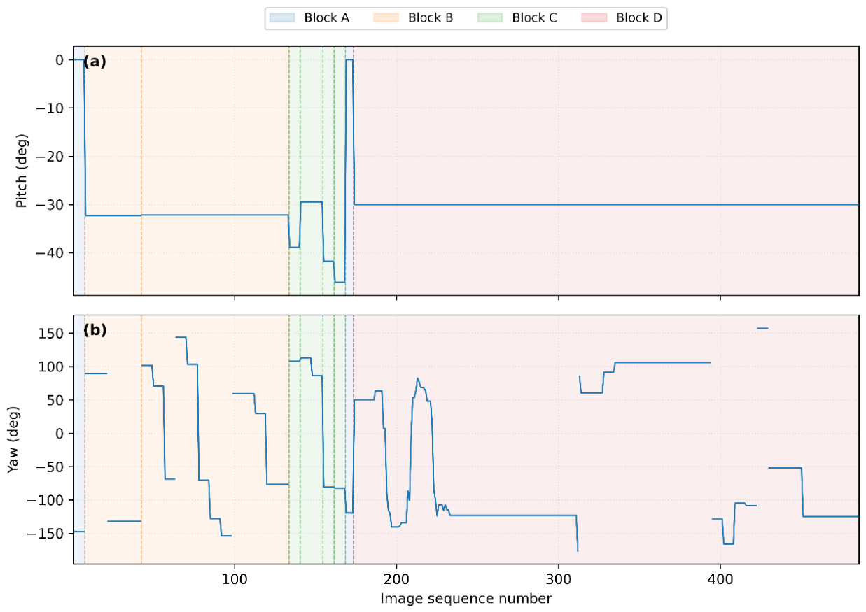
Figure 2.
Study area and network of ground control and check points. Ground control points (GCPs), check points (CPs), and points excluded after preliminary analysis of the photogrammetric project are shown.
Figure 2.
Study area and network of ground control and check points. Ground control points (GCPs), check points (CPs), and points excluded after preliminary analysis of the photogrammetric project are shown.
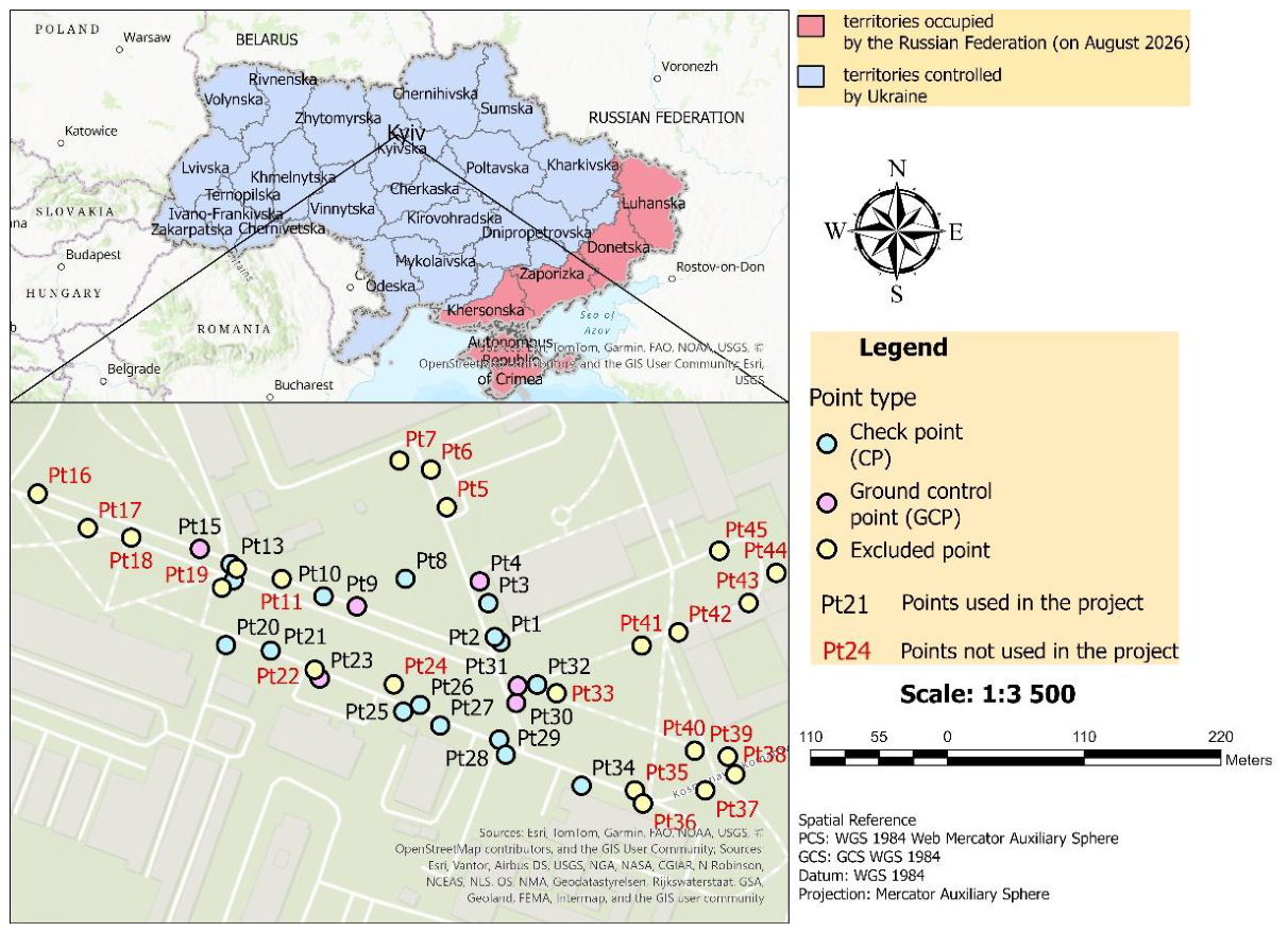
Figure 3.
Geometric characteristics of the 476 stereo pairs in experimental Blocks A–D: (a) full range of telemetry-derived inter-frame baselines and optical-axis angles; (b) enlarged view of the region with small baselines (≤ 2 m) and small optical-axis angles (≤ 5°). The optical-axis angle was calculated from telemetry-derived yaw and pitch using a convention independently validated against Pix4Dmapper camera orientations.
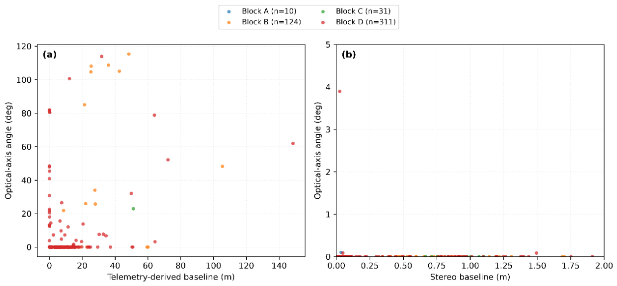
Figure 4.
Overall workflow of the proposed hierarchical Fourier–Mellin matching method and the independent evaluation framework.
Figure 4.
Overall workflow of the proposed hierarchical Fourier–Mellin matching method and the independent evaluation framework.
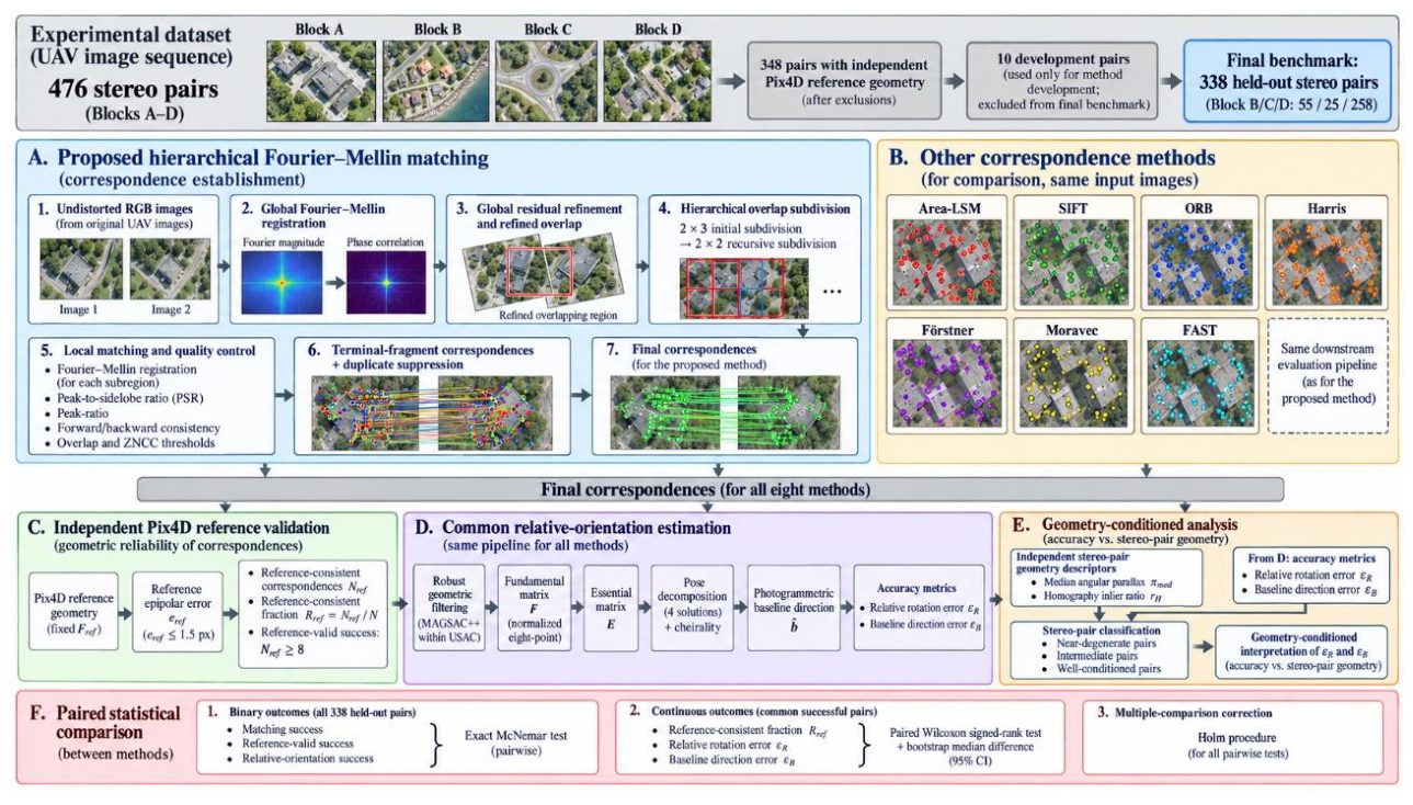
Figure 5.
Matching success and independent reference-valid success for the eight compared methods on the common held-out subset of 338 stereo pairs. Matching success denotes the presence of at least eight final correspondences; reference-valid success requires at least eight correspondences satisfying
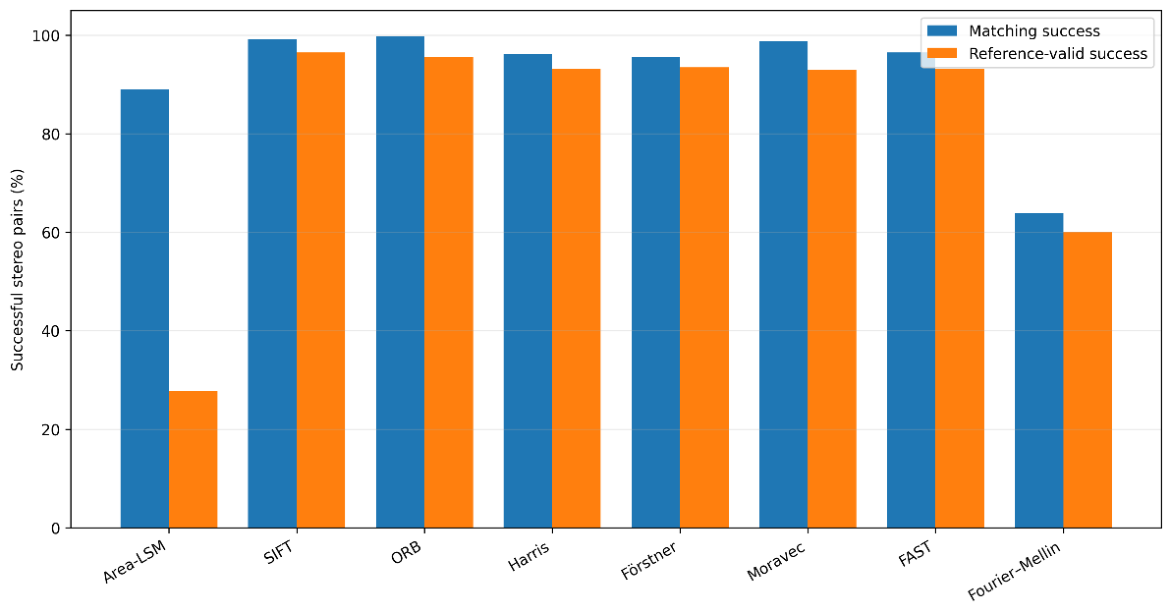
Figure 6.
Accuracy of relative orientation on successfully oriented held-out stereo pairs: (a) median and 95th percentile of the relative rotation error
Figure 6.
Accuracy of relative orientation on successfully oriented held-out stereo pairs: (a) median and 95th percentile of the relative rotation error
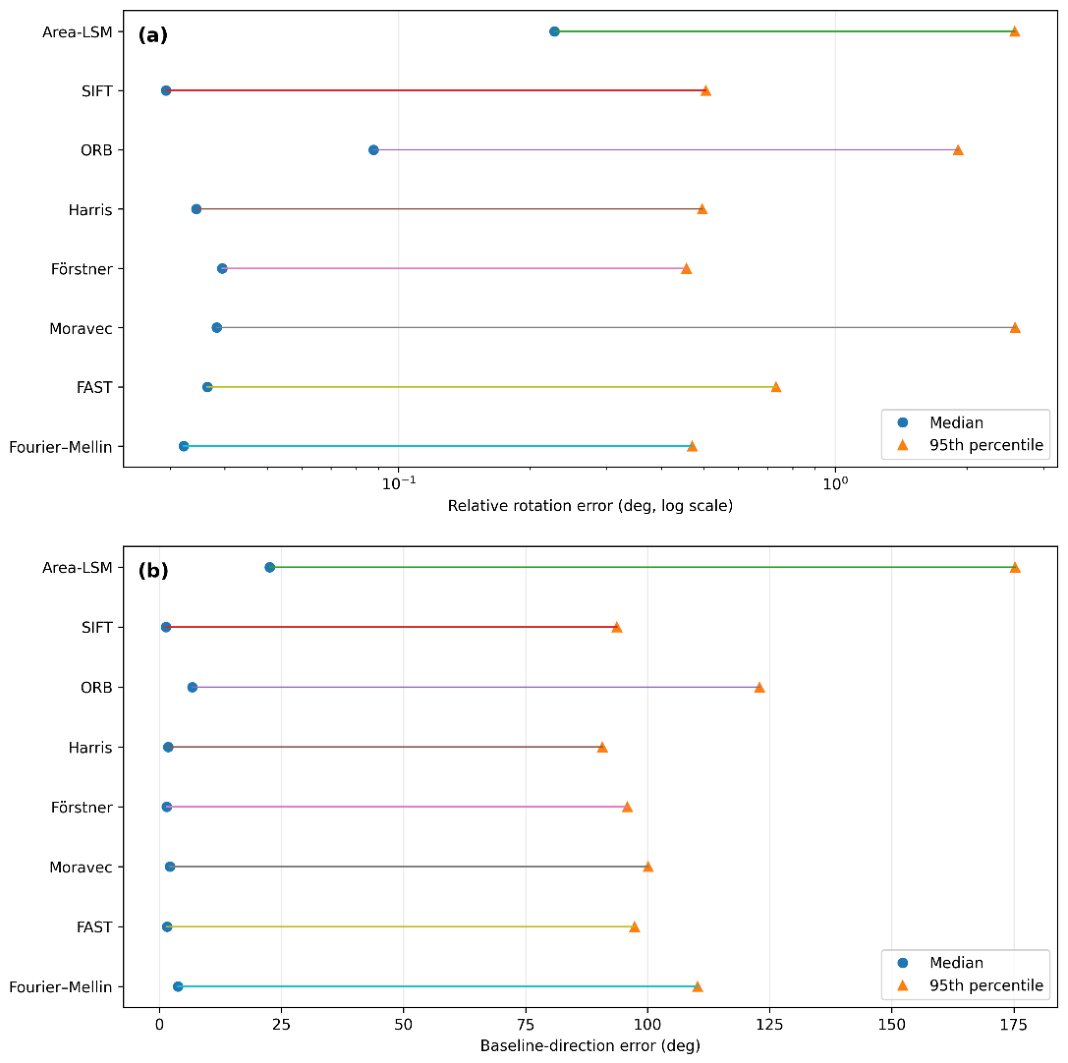
Figure 7.
Paired comparison of relative-orientation errors between the proposed Fourier–Mellin method and baseline methods on common successfully oriented held-out stereo pairs: (a) median paired difference in relative rotation error
Figure 7.
Paired comparison of relative-orientation errors between the proposed Fourier–Mellin method and baseline methods on common successfully oriented held-out stereo pairs: (a) median paired difference in relative rotation error
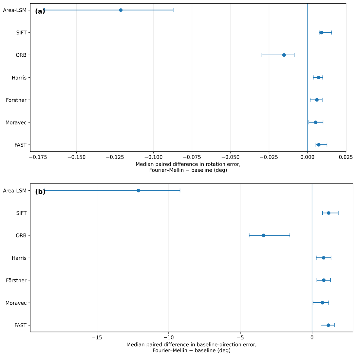
Figure 8.
Median baseline-direction error for the eight compared methods in near-degenerate, intermediate and well-conditioned stereo-pair regimes. The vertical axis is logarithmic because the baseline-direction error spans more than two orders of magnitude. Values are descriptive medians of successfully oriented pairs within each regime.
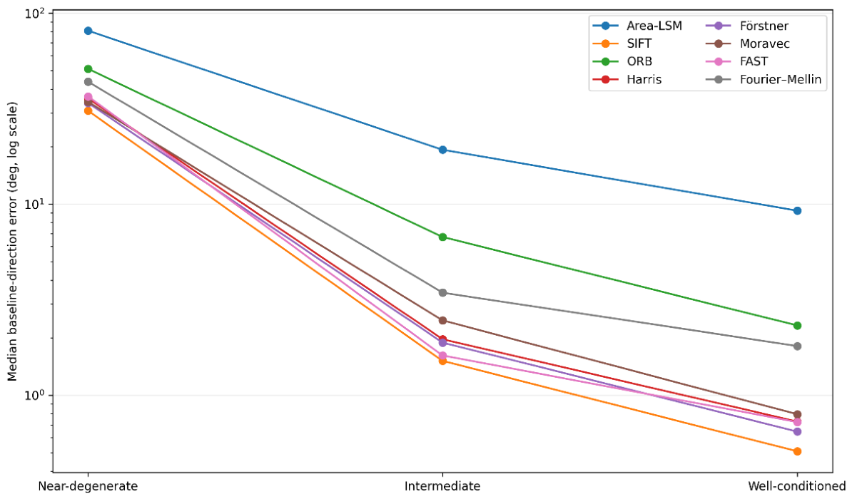

Table 1.
Initial and optimized camera interior orientation parameters obtained in Pix4Dmapper. The image resolution was 6144 × 4096 pixels. Values of σ represent the uncertainties of the estimated parameters.
Table 1.
Initial and optimized camera interior orientation parameters obtained in Pix4Dmapper. The image resolution was 6144 × 4096 pixels. Values of σ represent the uncertainties of the estimated parameters.
| Parameter | Initial value | Optimized value | σ |
| , px | 4915.200 | 5109.568 | 8.353 |
| , px | 3072.000 | 3090.678 | 11.746 |
| , px | 2048.000 | 2022.644 | 15.689 |
| 0 | −0.02239 | 0.006 | |
| 0 | 0.073032 | 0.026 | |
| 0 | −0.04647 | 0.036 | |
| 0 | −0.000476 | 0.001 | |
| 0 | 0.000291 | 0.001 |
Table 2.
Geometric characteristics of the experimental blocks.
| Block | Description | No. of pairs | Pitch | Mean baseline, m | Median baseline, m | Maximum baseline, m | Mean optical-axis angle, ° | Median optical-axis angle, ° | Maximum optical-axis angle, ° |
| A | Horizontal camera | 10 | 0.0° | 0.017 | 0.006 | 0.048 | 0.010 | 0.000 | 0.100 |
| B | Stable oblique acquisition | 124 | −32.2° | 4.716 | 0.000 | 105.442 | 6.312 | 0.000 | 115.326 |
| C | Transitional / higher-tilt segments | 31 | −46.1°… −29.5° |
1.937 | 0.000 | 51.174 | 0.740 | 0.000 | 22.927 |
| D | Main oblique survey segment | 311 | −30.0° | 6.223 | 1.247 | 148.460 | 4.019 | 0.000 | 113.912 |
Table 3.
Main implementation parameters of the feature-based methods.
| Parameter | Value | Parameter | Value |
| Maximum number of keypoints per image | 4000 | cornerSubPix maximum iterations | 30 |
| Minimum distance between Harris/Förstner/Moravec response maxima | 3 px | cornerSubPix epsilon | 0.01 px |
| Relative response threshold for Harris/Förstner/Moravec | 0.01 | SIFT ratio-test threshold | 0.75 |
| FAST threshold | 20 | ORB/Harris/Förstner/Moravec/FAST ratio-test threshold | 0.80 |
| ORB scale factor | 1.2 | RANSAC threshold | 1.5 px |
| ORB pyramid levels | 8 | RANSAC confidence | 0.999 |
| ORB patch size | 31 px | RANSAC maximum iterations | 10 000 |
| Harris/Förstner/Moravec/FAST descriptor size | 31×31 px | Minimum number of correspondences for fundamental-matrix estimation | 8 |
| cornerSubPix window | 5 px | ||
Table 4.
Matching performance and independent geometric consistency on the held-out subset.
| Method | Matching success, n (%) | Total final matches | Median final matches* | Reference-valid success, n (%) | Median reference-consistent fraction* |
| Area-LSM | 301 (89.05%) | 21,610 | 65.0 | 94 (27.81%) | 0.0588 |
| SIFT | 335 (99.11%) | 406,619 | 1310.0 | 326 (96.45%) | 0.9863 |
| ORB | 337 (99.70%) | 393,329 | 1169.0 | 323 (95.56%) | 0.9355 |
| Harris | 325 (96.15%) | 371,710 | 1197.0 | 315 (93.20%) | 0.9767 |
| Förstner | 323 (95.56%) | 377,386 | 1330.0 | 316 (93.49%) | 0.9760 |
| Moravec | 334 (98.82%) | 304,706 | 1014.5 | 314 (92.90%) | 0.9576 |
| FAST | 326 (96.45%) | 331,196 | 1173.0 | 315 (93.20%) | 0.9786 |
| Proposed Fourier–Mellin | 216 (63.91%) | 16,429 | 86.0 | 203 (60.06%) | 0.7865 |
* For stereo pairs satisfying the matching-success criterion.
Table 5.
Relative-orientation accuracy on the held-out subset.
| Method | Pose success, n (%) | Median, ° | , ° | Median , ° | , ° |
| Area-LSM | 300 (88.76%) | 0.2275 | 2.5781 | 22.6323 | 175.2492 |
| SIFT | 334 (98.82%) | 0.0293 | 0.5060 | 1.3440 | 93.7075 |
| ORB | 332 (98.22%) | 0.0876 | 1.9138 | 6.7725 | 122.8866 |
| Harris | 322 (95.27%) | 0.0344 | 0.4962 | 1.7847 | 90.7158 |
| Förstner | 321 (94.97%) | 0.0394 | 0.4566 | 1.5370 | 95.8179 |
| Moravec | 331 (97.93%) | 0.0383 | 2.5822 | 2.1556 | 100.0830 |
| FAST | 324 (95.86%) | 0.0365 | 0.7318 | 1.5925 | 97.2751 |
| Proposed Fourier–Mellin | 215 (63.61%) | 0.0322 | 0.4707 | 3.7987 | 110.2259 |
Table 6.
Paired statistical comparison of the proposed Fourier–Mellin method with baseline methods.
| Baseline | , pp (95% CI) | Common pose pairs | , ° (95% CI) | , ° (95% CI) | |||
| Area-LSM | +32.25 [26.33; 38.46] | 213 | −0.1212 [−0.1707; −0.0872] | −12.110 [−18.630; −9.200] | |||
| SIFT | −36.39 [−41.42; −31.36] | 215 | +0.0092 [0.0076; 0.0157] | +1.155 [0.728; 1.838] | |||
| ORB | −35.50 [−40.53; −30.47] | 214 | −0.0153 [−0.0295; −0.0086] | −3.378 [−4.384; −1.540] | |||
| Harris | −33.14 [−38.17; −28.11] | 215 | +0.0074 [0.0039; 0.0099] | +0.803 [0.299; 1.323] | 0.00212 | ||
| Förstner | −33.43 [−38.46; −28.40] | 215 | +0.0061 [0.0018; 0.0096] | 0.00172 | +0.812 [0.341; 1.290] | 0.00675 | |
| Moravec | −32.84 [−37.87; −27.81] | 215 | +0.0053 [0.0010; 0.0101] | 0.00513 | +0.718 [0.079; 1.156] | 0.01744 | |
| FAST | −33.14 [−38.17; −28.11] | 215 | +0.0073 [0.0056; 0.0127] | +1.138 [0.625; 1.570] |
Note: Δ = proposed Fourier–Mellin minus baseline. For, a positive value indicates a higher reference-valid success rate for the proposed method. For and , a negative value indicates a smaller error for the proposed method. All confidence intervals are paired-bootstrap 95% CIs.
Table 7.
Geometry-conditioned baseline-direction accuracy.
| Method | Near-degenerate: pose n (%) | Median, ° | Intermediate: pose n (%) | Median, ° | Well-conditioned: pose n (%) | Median, ° |
| Area-LSM | 52 (91.23%) | 80.896 | 116 (94.31%) | 19.255 | 130 (89.04%) | 9.245 |
| SIFT | 57 (100.00%) | 30.825 | 123 (100.00%) | 1.511 | 146 (100.00%) | 0.508 |
| ORB | 56 (98.25%) | 51.085 | 123 (100.00%) | 6.730 | 146 (100.00%) | 2.317 |
| Harris | 56 (98.25%) | 35.770 | 121 (98.37%) | 1.963 | 143 (97.95%) | 0.727 |
| Förstner | 55 (96.49%) | 33.872 | 121 (98.37%) | 1.885 | 143 (97.95%) | 0.645 |
| Moravec | 57 (100.00%) | 34.334 | 122 (99.19%) | 2.462 | 145 (99.32%) | 0.795 |
| FAST | 55 (96.49%) | 36.683 | 121 (98.37%) | 1.613 | 144 (98.63%) | 0.723 |
| Proposed Fourier–Mellin | 50 (87.72%) | 43.781 | 112 (91.06%) | 3.440 | 52 (35.62%) | 1.809 |
Disclaimer/Publisher’s Note: The statements, opinions and data contained in all publications are solely those of the individual author(s) and contributor(s) and not of MDPI and/or the editor(s). MDPI and/or the editor(s) disclaim responsibility for any injury to people or property resulting from any ideas, methods, instructions or products referred to in the content. |
© 2026 by the authors. Licensee MDPI, Basel, Switzerland. This article is an open access article distributed under the terms and conditions of the Creative Commons Attribution (CC BY) license (http://creativecommons.org/licenses/by/4.0/).
Copyright: This open access article is published under a Creative Commons CC BY 4.0 license, which permit the free download, distribution, and reuse, provided that the author and preprint are cited in any reuse.