

Submitted:
18 September 2026
Posted:
20 September 2026
You are already at the latest version
Abstract
Ground-point classification (GPC) is a fundamental step in LiDAR data processing because classification errors propagate into digital terrain models (DTMs), height normalization, vegetation structure metrics, and other derived products. Existing GPC algorithms depend on user-defined parameters whose effectiveness can vary with terrain complexity, vegetation structure, sampling density, and sensor-platform acquisition geometry. We present FAST-GC, a fully automated and self-tuning GPC algorithm that does not require scene-specific parameter calibration. FAST-GC was evaluated through complementary experiments encompassing a controlled six-site comparison with established ground-filtering algorithms, terrain-complexity and slope stress testing, systematic point-density reduction across 20 ALS sites, cross-platform ALS–ULS–TLS assessment, and large-area processing. Across the controlled comparative sites, FAST-GC maintained high ground completeness while limiting commission error, with its advantage over the established algorithms becoming increasingly pronounced as terrain complexity increased. At slopes of 70–80°, FAST-GC achieved a DTM mean absolute error (MAE) of 1.00 m compared with 3.12–12.75 m for the evaluated algorithms. Extended assessment across 20 ALS sites further demonstrated stable performance under systematic sampling-density reduction: reducing median density from 9.84 to 3.84 pts./m² maintained F1 ≈ 0.97, intersection over union (IoU) ≈ 0.95, and Matthews correlation coefficient (MCC) ≈ 0.85, while DTM MAE increased only from 0.07 to 0.11 m. Independently reconstructed 0.5 m terrain surfaces from ALS, ULS, and TLS observations showed strong cross-platform correspondence despite substantial differences in acquisition geometry and sampling conditions (R² and concordance correlation coefficient ≥ 0.99; RMSE = 0.10–0.16 m). Large-area processing of 382 ALS tiles (~23 km²) further demonstrated stable tile-wise execution and automated terrain-product generation. Collectively, the results show that GPC performance is governed not only by point-wise classification agreement but also by the ability to preserve terrain morphology under increasing topographic complexity, reduced sampling support, and contrasting acquisition geometries. By adapting terrain-support estimation internally rather than requiring scene-specific parameter calibration, FAST-GC provides a reproducible and scalable framework for heterogeneous and multi-platform LiDAR processing.
Keywords:
LiDAR
; ground point classification
; terrain modeling
; sensor-adaptive processing
; point-cloud processing
; digital terrain model
; ULS
; TLS
; ALS
1. Introduction
The use of Airborne Laser Scanning (ALS), and its sister technological niche—Unpiloted Aerial System Laser Scanning (ULS), Mobile Laser Scanning (MLS), Personal Laser Scanning (PLS), and Terrestrial Laser Scanning (TLS)—has significantly increased in recent years [1-4]. Laser scanners, whether deployed independently or concurrently in a multi-platform conundrum across aerial and terrestrial platforms, now provide unprecedented three-dimensional (3-D) information on terrestrial ecosystems, enabling advanced investigations in forest ecosystems [5,6], forest management [7], wildfire dynamics [8,9], terrain characterization [10], forest ecology [11], hydrology [12], and geomorphology [13,14].
To generate key LiDAR-derived products—Digital Elevation Models (DEMs), Canopy Height Models (CHMs), and Individual Tree Detection (ITD)—numerous parametric, machine learning (ML), and deep learning (DL) approaches have been investigated [15-19]. Among these approaches, ground points classification (GPC)—also termed bare-earth extraction—is a fundamental preprocessing step that isolates topography from off-terrain (OT) natural and man-made objects, such as vegetation and buildings [20-23]. The increasing availability of national-scale LiDAR datasets is enabling scientific analyses at spatial resolutions and extents that were previously unprecedented [24]. Due to the availability of higher sampling densities – Aggregate Nominal Point Density (ANPD) – greater than 2 pts/m², derived products (DEM, CHMs) with a resolution of 0.5 m have been developed [25]. Modern laser scanners – ALS, ULS, and TLS provide much higher ANPDs to generate high-resolution DEMs with cm-level resolution [14]. However, generating HR-DEMs at centimeter-scale spatial resolutions requires accurate GPC, which constitutes a critical preprocessing step for producing very high-resolution (VHR) downstream products, such as CHM and topographic derivatives, capable of capturing fine-scale terrain variability for applications in forestry and terrestrial ecosystem investigations [26,27].
1.1. Ground Classification Algorithms
Over the past three decades, several GPC algorithms have emerged and are widely implemented in software environments such as Point Data Abstraction Library (PDAL) – Python programming, and lidR – R programming [28-30]. These methods can be broadly categorized into distinct algorithmic families based on their underlying principles. Morphological filters, e.g., Progressive Morphological Filter (PMF)[31] and Simple Morphological Filter (SMRF), rely on structuring elements and elevation thresholding to separate ground from non-ground points. Surface-based and interpolation approaches, such as Progressive TIN Densification (PTD), iteratively construct and refine a terrain surface using geometric constraints. Curvature-based methods, notably Multiscale Curvature Classification (MCC)[13], exploit local surface curvature and scale-space analysis to distinguish terrain features. Physical simulation approaches, particularly the Cloth Simulation Filter (CSF) based GPC, use a mass–spring system that simulates a cloth draping over an inverted surface [32,33]. Additionally, slope- and elevation-threshold methods—such as modified slope-based filters (MSBF)[34] and extended local minimum (ELM) techniques [35]—apply heuristic rules based on local gradients [21].
Despite the methodological advances, GPC algorithm families are fundamentally built on assumptions of terrain continuity, elevation gradients, and neighborhood relationships [22,23,36,37]. Consequently, most approaches require explicit parameterization, including window size, slope thresholds, iteration limits, or stiffness coefficients, e.g., CSF [20,38,39]. A fundamental challenge is parameter sensitivity to topographic complexities, where optimal performance depends heavily on site-specific tuning, thereby reducing transferability across diverse forest ecosystems and topographic complexities [40-42]. Morphological, slope-based, and TIN-based ground filters remain sensitive to terrain complexity and initialization, as steep gradients, abrupt discontinuities, and errors in seed selection can propagate through the GPC process, whereas algorithms with several user-defined adaptive parameters require parameter tuning to maintain good performance across heterogeneous landscapes [33,43]. Nevertheless, most GPC algorithms were originally developed and tested using ALS, which typically exhibits relatively uniform sampling and moderate ANPD. When applied to cross-platform LiDAR modalities—including ULS, MLS, and TLS—these methods encounter additional challenges closely associated with sensor modalities rather than topographic regime [20,44-46]. These include heterogeneous point density, anisotropic sampling geometry, occlusion effects, and complex vertical structures [47,48]. To account for both topographic regime and sensor-related sensitivities, the parameter adjustment becomes significantly challenging when a ground truth or explicit accuracy validation is absent. Under such conditions, GPC algorithms are being used based on published resources where studies investigate the sensitivity of these parameters, along with providing optimized parameters through extensive trial-and-error analysis [22,48].
2. Materials and Methods
2.1. Workflow
At its core, FAST-GC implements a sensor- and data-driven GPC in which terrain-support criteria are automatically adjusted according to the LiDAR platform and the spatial sampling characteristics of the input point clouds. FAST-GC provides a modular workflow for LiDAR data processing (Figure 1). The available modules include: (a) input LAS/LAZ data cataloging, user-defined tiling, and tile-manifest generation; (b) sensor-aware FAST-GC ground classification for ALS, ULS, and TLS point clouds, followed by digital elevation/terrain model (DEM/DTM) generation and point-cloud height normalization; (c) spike-free digital surface model (DSM) generation (Khosravipour et al., 2016) [49] and merging of tile-wise outputs; (d) terrain and topographic derivatives, including slope, aspect, hillshade, curvature, terrain convergence index (TCI), and topographic wetness index (TWI); (e) canopy height model (CHM) generation using point-to-raster (p2r)[50], 99th-percentile (p99), pit-free CHM (Khosravipour et al., 2014) [51], percentile, percentile-top, and percentile-band approaches (fareed et. al., 2026); (f) ITD using Watershed (Vincent and Soille, 1991)[52] and (Yun et al., 2021) methods [53]; (g) forest structural metrics, including foliage height diversity (FHD) (MacArthur and Horn, 1969) ([54], vertical complexity index (VCI) [55], canopy cover (CC), standard deviation of height [z (SD)], number of points [Points (n)], and mean height (z mean); and (h) DEM of Difference (DoD) change detection (Wheaton et al., 2010) [56].
The modular workflow (Figure 1) is presented to provide users with an overview of the broader processing capabilities available within the FAST-GC Python package and is not individually evaluated in this study. The following subsections therefore focus specifically on the FAST-GC algorithm development and evaluation.
2.2. Tile-Enabled Fully Automated Workflow
FAST-GC is designed for large-scale LiDAR processing by partitioning input point clouds, provided either as individual files or collections of files, into user-defined tiles with spatial buffers. The buffers preserve neighboring-point support across tile boundaries and reduce edge artifacts during seamless merging of tiles to produce spatially continuous products (e.g., CHM, DSM, and DEM) in wide-area capacity [57]. Although spatial tiling is widely used in existing Python and R programming LiDAR packages, e.g., lidR [10], FAST-GC couples tiling with a persistent JSON manifest that records the processing configuration, input file sources, sensor mode, spatial extent, tile geometry, buffer size, point counts, point density (pts./m²), spatial occupancy, and support statistics required to reconstruct and manage the automated processing pipeline. Dataset-level summaries of tile sampling characteristics are additionally derived and used by FAST-GC to adapt selected internal processing scales when local sampling support deviates substantially from the overall dataset, thereby accommodating variations associated with sensor sampling and spatial heterogeneity. An additional safeguard is applied to incomplete terminal tiles generated along dataset boundaries. Small edge fragments and geometrically narrow sliver tiles are identified during tile planning and automatically consolidated with adjacent spatial tiles before the point-cloud tiles are written – a unique feature that is available in FAST-GC to avoid any data loss during tile processing.
2.3. Algorithm Design and Mathematical Background
FAST-GC is conceptually motivated by CSF in the inverted point-cloud 3D domain [58,59]. In CSF, the point clouds are inverted using point elevation (z), and a simulated cloth is allowed to conform to the inverted surface [59]. FAST-GC retains inversion as a useful geometric transformation but replaces cloth simulation with deterministic reconstruction of an observed terrain-support manifold – a thin membrane of topographic surface by separating it from off-the-terrain objects (OT). FAST-GC accomplishes this using three tiers of information directly from point clouds to operate without user-defined parameterization over complex topographic regimes: (i) Input sensor mode, which defines the nature of the sensor-platform, is followed by (ii) statistical information directly obtained from tiles; and (iii) automatic derivation of the operational parameter initiation in 3D inverted space to deal with point densities, occlusion, and height range in each tile to facilitate statistical inference in inverted 3D space.
FAST-GC begins with sensor-specific baseline configurations for ALS, ULS, and TLS, but adapts the spatial support scale to the sampling characteristics of individual input point-cloud tiles. Let sddenote the dataset-level scale selected from the observed support-density regime. A bounded tile-level adjustment, Δst, is subsequently derived from the relative local support of the tile, including the median point count and occupancy of 2-m grid cells and, where required, point density. The effective support scale, st, is
where sminand smaxare sensor-specific bounds. Thus, sparsely supported tiles receive a modest increase in spatial support, whereas exceptionally dense tiles permit a smaller support scale. Selected spatial support parameters are then adapted from their sensor-specific baseline values (Equation 2).
where h0and n0 are the baseline voting-cell size and minimum number of supporting neighboring cells, respectively; h is the adapted horizontal cell size; and nL and nU define the allowable sensor-specific support range. Candidate-cell size and other spatial support distances are adapted analogously within bounded ranges. This procedure changes the spatial scale of evidence collection without altering the underlying classification logic. Let the input point cloud be.
where xi and yi denote horizontal coordinates and zi is the original elevation of return i. FAST-GC constructs the initial terrain support in an inverted vertical space, such that low-elevation returns in the original point cloud become upper-envelope observations after inversion. Using a reference elevation zref, the inverted elevation of point ican be expressed as
where denotes the inverted elevation. Because this transformation reverses vertical ordering, a point with the lowest original elevation zi has the highest inverted elevation which can be presented as
st = clip(sd + Δst, smin, smax)
The horizontal domain is partitioned into cells of width h. Within each occupied cell c, FAST-GC selects the point having the maximum elevation as the initial terrain candidate – theoretically, a candidate point in the given cell with the highest probability of being a legitimate ground point,
where is the index of the selected candidate points and is its elevation in inverted space. To reduce dependence on the arbitrary position of the grid origin, candidate selection is repeated using a second grid displaced by one-half of the cell width along both horizontal axes, as presented as:
This produces a second set of inverted-space candidates, . After mapping the offset-grid candidates to the base grid, the two candidate layers are combined by retaining the upper support envelope in inverted space.
For cells in which both candidate points are available from both layers, the point with the highest elevation is retained, whereas the available point is used when only one grid contributes support, given that one of the layers contains empty grid cells. The half-cell displacement provides an alternative spatial partition for returns located near base-grid boundaries and thereby reduces grid-origin sensitivity and compensates for the empty grid cells originating from the base layer. The combined provisional support is subsequently anchored to their original locations as candidate ground seeds in unclassified point clouds. For each base-grid cell c, FAST-GC selects the points whose inverted elevation is closest to the provisional support. :
where is the index of the selected return and is its snapped elevation in inverted space. This snapping operation constrains the support layer to elevations represented by actual LiDAR returns before terrain voting. FAST-GC next evaluates whether each snapped support is consistent with its surrounding terrain. Let c(R) denote the square neighborhood surrounding cell c, where R is the half-width of the square voting neighborhood, expressed in grid cells.
where represents the local center of the inverted terrain-support elevations, is their unscaled median absolute deviation (MAD), and dmin prevents the robust dispersion estimate from collapsing in locally uniform terrain. A neighboring support contributes to the terrain vote when
where kMAD controls the allowable standardized deviation and 1.4826 provides the conventional Gaussian-consistent scaling of MAD. If at least nminneighboring support cells satisfy Equation (11), the voted terrain-support elevation in inverted space at cell c is estimated as.
Grid cells lacking a valid terrain estimate after neighborhood voting are iteratively filled from neighboring finite terrain estimates using a 3 × 3 median neighborhood, after which NaN-aware separable smoothing is applied to obtain the continuous inverted terrain membrane. The resulting membrane is then transformed back to the original elevation space as:
here is the reconstructed terrain membrane in the original coordinate system. Importantly, the voting stage suppresses isolated low or high observations before surface completion, thereby reducing the influence of vegetation returns and other vertically inconsistent support. The reconstructed membrane is bilinearly sampled at the horizontal position of each return, and its signed vertical residual is defined as:
where positive residuals represent returns above the estimated terrain and negative residuals represent returns below it. Rather than applying a globally fixed elevation threshold, FAST-GC adjusts the admissible residual according to local terrain geometry:
where τ0 is the baseline vertical tolerance, ks is the slope-adaptation coefficient, is the local terrain-gradient magnitude, and bi is a bounded allowance associated with abrupt local terrain transitions. The latter is derived from local breakline relief.
where ρi is the bilinearly sampled relief at point i. Unlike curvature, ρi retains units of elevation and represents local departures from the surrounding terrain surface at crests, concavities, and slope transitions. Initial ground membership is then assigned using an asymmetric residual interval.
where denotes initial ground membership. The asymmetric interval permits greater downward deviation from the reconstructed terrain membrane than upward deviation while maintaining a stricter constraint against above-terrain returns. The initial terrain classification is subsequently refined using a sequence of spatial-consistency tests designed to address terrain voids, depressions, locally weak ground support, canopy leakage, isolated ground labels, and tile-edge inconsistencies. These operations use the already reconstructed terrain membrane and neighboring point evidence rather than introducing an independent classification model. Recovery is therefore restricted to points that exhibit sufficient local terrain support, while contamination guards remove ground labels that are vertically or spatially inconsistent with the surrounding terrain manifold. Detailed formulations and parameter bounds for these refinement operations are provided in Supplementary (Note S1).
τi = clip(τ0, + , ks gi + bi , τmin,τmax)
Computational performance of FAST-GC was evaluated using a large-area ALS dataset comprising 382 spatial tiles (250 × 250 m), corresponding to a nominal processing footprint of ≈23 km². Processing was performed on a 64-bit Windows 11 system equipped with a 12th-generation Intel Core i9-12900H processor (2.50 GHz) and 32 GB RAM. FAST-GC was executed using 16 parallel CPU workers with the loky multiprocessing backend. Spatial processing used a 5 m tile buffer, and DEM and CHM products were generated at 0.5 m spatial resolution. Computational performance was evaluated independently for GPC, DEM generation, height normalization, and CHM generation. Processing efficiency was characterized using wall-clock processing time, mean processing time per tile, and nominal-area throughput where complete stage-level timing was available. Area-based throughput was calculated from the nominal 250 × 250 m tile footprint and therefore represents computational processing coverage rather than the exact unique geographic extent of the ALS acquisition (for details, see Section 3.6).
2.4. Benchmark and Cross-Validation Datasets
For GPC quantitative evaluation, the principal benchmark was assembled from the ALS dataset of Jin et al. (2020), acquired in the southern Sierra Nevada Mountains, California (CA), USA [17]. The original dataset comprised twenty 500 × 500 m sites distributed among four study areas: Providence, San Joaquin Range, Courtwright Road, and Wolverton–Tokopah. The region encompasses substantial topographic variation and mixed-conifer forest dominated by white fir (Abies concolor), ponderosa pine (Pinus ponderosa), and incense cedar (Calocedrus decurrens), with black oak (Quercus kelloggii) and canyon live oak (Quercus chrysolepis). Across the twenty original sites, mean canopy cover ranged from 0 (non-forested) to 90%, mean tree height from 0 to 25.9 m, mean elevation (m.a.s.l.) from 426 to 3347 m, and mean terrain slope from 6.0° to 41.5° [17].
The ALS data was acquired in August 2010 using an Optech GEMINI Airborne Laser Terrain Mapper (ALTM) mounted on a twin-engine Piper PA-31 Chieftain. The system was operated at a pulse repetition rate of 100 kHz and a scanning frequency of 50 Hz, with a ±14° scan angle and a single-swath width of 233.26 m. Adjacent swaths overlapped by more than 50%, and the sensor recorded up to four echoes per emitted pulse. The mean point density across the acquisition was approximately 10.27 pts m⁻². Independent vertical assessment was conducted by the data provider using 243 road checkpoints collected with a vehicle-mounted GPS; the reported RMSE of LiDAR elevations relative to these checkpoints was 0.024 m and was described as spatially homogeneous among the study sites.
A five-site subset was assembled for the controlled benchmark following a similar approach over the same geographic region [43]. To avoid confusion between the numbering used here and that of the source dataset, the selected blocks were renumbered as FAST-GC benchmark Sites 1–5 (Table 1). Benchmark Site 1 combines source blocks 6 and 8 of Jin et al., whereas benchmark Sites 2–5 use source blocks 1, 12, 13, and 15, respectively (Table 1). Hereafter, all site numbers refer exclusively to the FAST-GC benchmark numbering unless explicitly stated otherwise. The subset was selected to represent contrasting sources of ground-classification difficulty and canopy cover conditions (see Figure 2).
Site 1 represents the vegetation-dominated end of the benchmark (Figure 2a). Its two constituent forest blocks have mean canopy cover of 72% and 54%, mean tree heights of 24.9 and 13.7 m, and mean terrain slopes of 15.8° and 12.4°, respectively. In the combined benchmark point cloud, only 40.36% of points are reference ground, providing a strong test of ground discrimination where non-ground returns are abundant. Site 2 represents an intermediate vegetation–terrain condition, with 30% mean canopy cover, 10.3 m mean tree height, 17.1° mean slope, and 69.09% reference ground (Figure 2b).
The dominant filtering challenge changes substantially at Sites 3 and 4. These sites contain 96.86% and 98.26% reference ground, respectively, while mean canopy cover decreases to 17% and 1% (Figure 2c, d). Their terrain, however, is considerably more demanding: mean slopes are 36.1° and 28.2°, with maximum slopes reported by Jin et al. of 88.3° and 87.1°, respectively. These sites therefore provide particularly useful tests of whether a GPC can retain legitimate ground across steep and rapidly varying terrain with minimal vegetation. Site 5 combines both sources of complexity. It has 29% mean canopy cover and 41.5° mean terrain slope—the highest mean slope among the selected benchmark sites—while the distributed point cloud spans approximately 579 m in elevation within 0.25 km² (Figure 2e). The five-site design consequently encompasses vegetation-dominated, intermediate, exposed steep-terrain, and combined vegetation–extreme-terrain conditions rather than relying solely on differences in ground/non-ground class proportions.
Reference-label quality was an additional reason for selecting these data for the principal evaluation. Authors first generated preliminary ground classifications using TerraScan and subsequently inspected the classified point clouds manually using cross-sectional visualization in LiDAR360 [17]. Erroneously classified points were corrected, and additional legitimate ground points were recovered during this procedure. For the six source blocks used in the present benchmark, the reported proportions of manually corrected points were 10.99%, 13.18%, 14.44%, 25.44%, 0.12%, and 33.61% for source blocks 1, 6, 8, 12, 13, and 15, respectively. These correction rates further indicate substantial differences in the original filtering difficulty among the selected landscapes.
In addition to the principal-controlled ALS benchmark, three complementary datasets were used to examine aspects of FAST-GC performance that could not be assessed from the benchmark alone.
First, selected scenes from the OpenGF benchmark (Sites 6 – 7) were used as external stress tests under environmental conditions distinct from the principal benchmark [60]. OpenGF is a large-scale ALS ground-filtering dataset containing more than 542 million labeled points over more than 47 km² and representing nine terrain-scene types across four countries. An urban scene was included because built environments provide comparatively well-defined exposed surfaces for examining classification behavior in a setting outside the primary design domain of FAST-GC, which is unbuilt terrestrial landscapes (Site 6, Table 1). Mountainous forest scenes were additionally used to evaluate performance under complex terrain and sparse ground-returning conditions. Quality-control inspection of these scenes (Site 7), including profile/transect-based examination, indicated that the supplied ground labels could represent a comparatively conservative delineation by only incorporating, as reported by the authors, “high-quality ground labels”. Consequently, OpenGF was retained as an operational external reference rather than treated as equivalent to the manually reviewed principal Jin et al. benchmark. Performance was therefore examined in two complementary ways: (i) conventional point-wise comparison of FAST-GC, PMF, CSF, and PTD against the high-quality OpenGF ground labels and (ii) pairwise comparison among the independently generated GPCs to determine whether apparent disagreement with the high-quality OpenGF ground labels was also reflected in disagreement among the algorithms themselves.
Second, multi-platform data from the central European forest dataset of Weiser et al., 2022a were used to evaluate cross-platform consistency among independently acquired ALS, ULS, and TLS observations [61,62]. The dataset comprises 12 forest plots in Bretten and Karlsruhe, Baden-Württemberg, Germany, with spatially overlapping acquisitions from ALS, ULS, and TLS platforms. Because the existing point classifications were not generated specifically as manually validated ground-filtering reference data, these data were used primarily to assess whether FAST-GC could reconstruct spatially consistent HR-DEM terrain surfaces under substantially different acquisition geometries and sampling distributions rather than for conventional point-wise accuracy benchmarking. Site 8 in this study comprised plot “BR01” containing ALS, ULS, and TLS datasets.
Third, a spatially extensive ALS dataset from the Lubrecht Experimental Forest, Montana, USA, was used to assess the landscape-scale processing stability of FAST-GC and the spatial consistency of the resulting terrain reconstruction (Site 9). The original survey was acquired by Quantum Spatial for the University of Montana during 27–30 June 2015 using a Leica ALS70 sensor operated at approximately 1400 m above ground level. The complete acquisition encompassed 61,237 acres and achieved an average first-return density of 20.07 pts m⁻² [63]. The Lubrecht Experimental Forest represents a topographically heterogeneous mixed-conifer landscape in western Montana, providing extensive variation in terrain, canopy cover, and ground-return availability [63-65]. For the present study, an approximately 23 km² subset of the available ALS coverage was used as a large-area evaluation dataset. Unlike the smaller datasets used for point-wise accuracy assessment, this dataset was intended to examine whether FAST-GC could be applied systematically at landscape scale while maintaining spatially coherent terrain reconstruction.
2.5. Evaluation Approaches
To benchmark the performance of FAST-GC, a comprehensive review of the existing literature was conducted to identify widely used and well-established GPC algorithms [60,66]. The selection was guided by three key criteria. First, the algorithms are implemented in open-source environments, ensuring accessibility and reproducibility for the broader research community [10,48,67]. Second, the selected methods represent distinct and widely recognized GPC algorithm families, enabling a balanced and meaningful comparison [30]. Based on these criteria, the performance of FAST-GC was evaluated against three representative approaches: CSF, PMF, and PTD – all of which are implemented and available in the lidR package [10]. Finally, given the reason that all three above-mentioned GPC algorithms have been extensively applied and validated in prior studies to classify point clouds from ALS, ULS, and TLS, as evidenced by their frequent use in published literature e.g., CSF, PMF, and PTD, therefore qualified for comparison [30,60,68-70].
Point-based GPC performance was evaluated using binary reference labels, with ground treated as the positive class and non-ground as the negative class. Performance was quantified using intersection over union (IoU), precision, recall, F1-score, Matthews’s correlation coefficient (MCC), omission error (OE), and commission error (CE) (Equations 18–24). IoU was calculated for the ground class. Precision and recall quantify the purity and recovery of predicted ground points, respectively, while F1-score summarizes their balance. MCC incorporates all four components of the binary confusion matrix and provides a complementary measure of classification agreement under class imbalance. OE represents the proportion of reference ground points omitted from the predicted ground class, whereas CE represents the proportion of predicted ground points labeled as non-ground in the reference. Here, TP, FP, TN, and FN denote true-positive, false-positive, true-negative, and false-negative points, respectively [71].
IoU = TP / (TP + FP + FN)
Precision = TP / (TP + FP)
Recall = TP / (TP + FN)
F₁ = (2 × Precision × Recall) / (Precision + Recall) = 2TP / (2TP + FP + FN)
MCC = (TP·TN − FP·FN) / √[(TP + FP)(TP + FN)(TN + FP)(TN + FN)]
OE = [FN / (TP + FN)] × 100 = (1 − Recall) × 100
CE = [FP / (TP + FP)] × 100 = (1 − Precision) × 100
For the Jin et al. ALS benchmark, the supplied ground/non-ground labels were used as the principal reference for quantitative evaluation. FAST-GC, PMF, CSF, and PTD predictions were compared point-by-point against the same reference labels using the metrics defined above. This evaluation constituted the principal-controlled comparison of ground-classification performance and was used to examine algorithm behavior across the represented forest and terrain conditions.
The OpenGF evaluation was treated separately because it served as an external benchmark and stress test rather than as an extension of the principal-controlled ALS evaluation. All four algorithms were first evaluated against the supplied OpenGF ground/non-ground labels using the same point-wise metrics, thereby preserving direct comparison with the published benchmark reference. The supplied labels were therefore retained unchanged as the external reference, but the resulting reference-based metrics were interpreted together with a second, reference-independent analysis. Pairwise positive agreement among FAST-GC, PMF, CSF, and PTD classifications was calculated to determine the extent to which independently applied algorithms identified a common ground-point population. This complementary analysis was not used to establish ground-truth correctness; rather, it provided a means of distinguishing disagreement specific to the supplied reference from broader disagreement among the independently generated classifications.
Because point-wise classification performance does not directly quantify the geometric fidelity of the reconstructed terrain, terrain-surface performance was evaluated independently using HR-DEM at 0.5 m resolution. For nspatially corresponding DEM cells, the elevation residual was defined as ei = zi, pred − zi, ref. Reference-based DEM accuracy was quantified using bias, mean absolute error (MAE), root mean square error (RMSE), and the 95th percentile of absolute error (P95) (Equations 25–28). Bias represents systematic vertical displacement, MAE represents the magnitude of absolute vertical error, RMSE gives greater weight to larger deviations, and P95characterizes the upper tail of the absolute-error distribution [70].
For cross-platform terrain-surface comparisons, normalized bias (nBias), coefficient of determination (R2), concordance correlation coefficient (CCC), and normalized median absolute deviation (NMAD) were additionally calculated (Equations 25–32).
Bias = (1/n) Σᵢ₌₁ⁿ eᵢ
MAE = (1/n) Σᵢ₌₁ⁿ |eᵢ|
RMSE = √[(1/n) Σᵢ₌₁ⁿ eᵢ²]
P₉₅ = Q₀.₉₅(|eᵢ|)
nBias (%) = 100 × Bias / z̄ref
R² = 1 − [Σᵢ₌₁ⁿ(yᵢ − ŷᵢ)² / Σᵢ₌₁ⁿ(yᵢ − ȳ)²]
CCC = 2 Cov(x,y) / [Var(x) + Var(y) + (x̄ − ȳ)²]
NMAD = 1.4826 × median(|eᵢ − median(eᵢ)|)
These metrics characterize relative vertical bias, linear correspondence, concordance, and robust residual dispersion, respectively. Cross-platform statistics were interpreted as measures of terrain-surface consistency rather than absolute accuracy because the independently acquired ALS, ULS, and TLS datasets do not provide a common point-wise benchmark or HR-DEM [62].
3. Results
3.1. ALS Ground-Classification Benchmark
For comparison, the GPC algorithms were applied using a single fixed parameterization across all benchmark sites: PTD (th1 = 1.2, th2 = 0.1, tol = 10, max_edge = c(0, 1.5), and n = 8), PMF (window sizes = 3, 6, 9, and 12 m; corresponding elevation thresholds = 0.10, 0.57, 1.03, and 1.50 m), and CSF (slope smoothing = TRUE, classification threshold = 1.0 m, cloth resolution = 1.0 m, rigidness = 1, maximum iterations = 500, and time step = 1.0) [70,72]. These configurations were selected from documented ALS implementations and literature-supported operating ranges rather than optimized separately for individual sites [10]. Because the benchmark encompasses contrasting conditions ranging from dense canopy conditions (Sites 1 – 2), moderate-terrain environments to steep and strongly varying topography (Sites 3 – 5), the same parameterization was retained across all sites to provide a reproducible common operating configuration. Point-wise classification performance was evaluated on five controlled ALS benchmark sites (Table 1, Figure 2) using identical operational settings for all methods (250 m processing tiles/chunks with a 5 m buffer). FAST-GC was compared with PTD, CSF, and PMF. Table 2 reports Precision, Recall, F1-score, intersection over union (IoU), Matthews correlation coefficient (MCC), commission error (CE) %, and omission error (OE) %.
Across the five controlled ALS benchmark sites, FAST-GC achieved the strongest overall point-wise ground-classification performance, with macro-average Recall, F1-score, IoU, and MCC of 0.96, 0.98, 0.96, and 0.81, respectively (Table 2). Precision remained close to 1.00 for all methods, indicating that differences among algorithms were driven primarily by their ability to retain legitimate reference-ground points rather than by excessive classification of non-ground points as ground. FAST-GC maintained a macro-average CE of 0.35%, while OE was 3.36%. Among the reference algorithms, CSF was the strongest overall competitor, with macro-average F1-score, IoU, and MCC of 0.92, 0.86, and 0.63, respectively, followed by PMF and PTD. PTD produced the lowest CE (0.06%) but also the largest OE (23.12%), indicating a comparatively conservative classification response that minimized false ground assignments at the cost of substantial ground omissions.
The performance pattern differed systematically with terrain and vegetation setting. Sites 1 and 2 represent the more strongly forested benchmark conditions (Table 1; Figure 2a,b) but differ in ground availability and terrain structure. Site 1 contained 59.64% non-ground returns and dense canopy structure over locally steep terrain, whereas Site 2 had a larger ground fraction (69.09%) and represented a more balanced vegetation–terrain setting. Under these conditions, CSF and FAST-GC showed comparable performance. At Site 1, CSF achieved F1, IoU, and MCC values of 0.99, 0.97, and 0.98, respectively, compared with 0.98, 0.96, and 0.96 for FAST-GC. At Site 2, both methods achieved F1 ≈ 1.00 and IoU ≈ 0.99, with PMF also maintaining high performance. In contrast, PTD recall was 0.82 at both sites, corresponding to OE values of 18.46% and 17.96%, respectively. These results indicate that under forested conditions with substantial canopy returns, both FAST-GC and CSF maintained effective ground recovery, while the substantially higher omission rates of PTD reflected a more conservative ground classification response [73].
The relative performance changed substantially at Sites 3 and 4, where ground returns constituted 96.86% and 98.26% of the point clouds, respectively, and the principal classification challenge was associated with steep and strongly varying terrain rather than dense vegetation (Table 1; Figure 2c, d). FAST-GC maintained the strongest overall performance under these conditions, with recall of 0.96 and 0.97 and F1-scores of 0.98 and 0.99 at Sites 3 and 4, respectively, while limiting OE to 3.81% and 2.89%. CSF was the closest reference method at both sites, but its recall declined to 0.79 and 0.85, corresponding to substantially higher OE values of 20.99% and 14.73%. PTD and PMF were similarly omission-prone; at Site 4, both achieved a recall of 0.75 with approximately 25% OE, while at Site 3 PMF showed the lowest ground retention (recall = 0.72; OE = 28.32%). These results are consistent with the sensitivity of conventional filtering approaches to steep slopes and rapidly varying terrain. Progressive TIN densification can perform well in mountainous terrain but depends strongly on the quality of initial terrain seeds and parameter thresholds [32], while CSF can provide a high-quality initial terrain yet may misclassify points during refinement in steep mountainous areas. Forest-focused comparisons have likewise reported smoothing or omission of steep terrain by PMF and PTD and increased vegetation-related commission by CSF under complex conditions [41,73].
Site 5 represents the combined challenge of substantial vegetation and extreme terrain relief, with 21.76% non-ground returns and an elevation range of approximately 579 m (2175.60–2754.79 m; Table 1; Figure 2e). FAST-GC maintained the strongest overall performance under these conditions, with recall of 0.932, F1-score of 0.96, IoU of 0.92, and MCC of 0.85, while limiting OE to 6.82%. CSF and PTD showed nearly identical F1-score and IoU values (0.82 and 0.69, respectively), indicating similar deterioration in ground retention, whereas PMF showed the greatest ground loss, with recall of 0.63, F1-score of 0.77, and OE of 37.35%[74]. The substantially higher omission rates of the GPC algorithms under the combined terrain–vegetation effect indicate increasing difficulty in retaining ground returns as surface complexity increases. This pattern is consistent with previous forests benchmarking studies reporting that morphological approaches can omit substantial ground in structurally complex environments and that GPC algorithms' performance depends strongly on terrain form, canopy conditions, and parameter optimization [74].
The error distribution in Figure 3 further explains the divergence among GPC algorithms as terrain complexity increased. Across Sites 3–5, FAST-GC maintained high ground retention, with TPR ranging from 93.2% to 97.1% and OE from 2.89% to 6.82%, while maintaining low commission error (0.04–0.33%). In contrast, the reference algorithms generally retained very low commission error but showed pronounced reductions in TPR, indicating that their declining F1-score and IoU were driven primarily by omission of reference-ground points rather than increased acceptance of non-ground points. This behavior was most evident at Site 5, where OE increased to 30.38%, 31.00%, and 37.35% for CSF, PTD, and PMF, respectively, compared with only 6.82% for FAST-GC. The very low CE of PTD and PMF therefore reflects, in part, a more conservative classification approach characterized by higher ground omission rather than uniformly improved ground/non-ground discrimination.
Collectively, Table 2 and Figure 3 show that differences among GPC algorithms became more pronounced as terrain complexity increased. While FAST-GC and CSF performed comparably under dense canopy conditions (Sites 1–2), FAST-GC maintained substantially higher ground retention across the steep and topographically complex areas (Sites 3–5), with substantially lower OE than the counterparts – CSF, PMF, and PTD.
3.2. Urban Test Site
An additional OpenGF ALS (Site 6) was used to evaluate GPC in urban terrestrial ecosystems. Site 6 represents a distinct landscape characterized by gentle terrain together with buildings and other urban surface structures.
CSF achieved the highest overall classification agreement on the urban site, with an F1-score of 0.95, IoU of 0.91, and MCC of 0.92. FAST-GC achieved an F1-score of 0.92, IoU of 0.86, and MCC of 0.87, while retaining nearly all reference ground (Recall = 0.99; OE = 0.27%). Its Precision of 0.86 and CE of 13.17% indicate that errors were dominated by non-ground points assigned to the ground class rather than omission of reference ground (Table 3). On the contrary, some studies reported the weakest performance in urban contexts, which indicates that urban contexts are more complex and CSF accuracy is therefore subject to the urban sites' complexity [30].
The reference algorithms exhibited different error characteristics. PTD produced the highest Precision (0.95) and lowest CE (4.72%), but its Recall decreased to 0.84, resulting in an OE of 15.92%. In contrast, PMF produced the highest Recall and lowest OE (<0.01%) but also the highest CE (22.45%), resulting in lower overall agreement (F1 = 0.87; MCC = 0.78). The urban evaluation therefore shows a clear variation in the balance between GPC and non-ground rejection: CSF provided the strongest overall agreement, FAST-GC strongly preserved reference ground with moderate commission, PTD favored non-ground rejection at the expense of ground omission, and PMF maximized ground retention but introduced substantially greater commission.
3.3. Qualitative Analysis
Qualitative assessment of high-resolution (HR) 0.5 m DEM (Figure 4) showed that all four methods reproduced the broad terrain morphology of Sites 2–5, yet substantial differences were evident in the spatial extent and continuity of HR-DEM residuals relative to the reference surface (see red polygons in Figure 4). On Site 2, DEM reconstruction was highly consistent among all algorithms, with only small and spatially isolated regions exceeding the ±0.25 m DoD threshold set as an evaluation criterion. This agrees with the relatively favorable classification performance observed for this site and indicates that differences in classified ground points had limited influence on the reconstructed terrain surface, given that the topographic complexity is favorable for all GPC algorithms with gentle slope transitions.
However, DoD became substantially more pronounced for all algorithms on Sites 3–5. FAST-GC generally preserved the major landforms while limiting DoD to comparatively localized areas (red polygons in Figure 4). In contrast, CSF, PTD, and particularly PMF produced larger and more spatially connected residual regions in the more topographically complex areas. The DoD is especially apparent along steep terrain transitions, ridges, drainage features, and sharp changes in local relief, where the red residual boundaries become increasingly extensive. On Sites 3 and 4, the reference-scale terrain structure remains visually continuous in the FAST-GC DEM, whereas CSF, PMF, and PTD DoDs contain broader zones exceeding the 0.25 m threshold. Site 5 produced the greatest disagreement among algorithms, with extensive residual regions occurring across the major terrain break and adjoining steep surfaces.
Overall, the spatial DoD patterns indicate that the principal advantage of FAST-GC was not simply preservation of the overall elevation gradient, which was reproduced by all methods, but improved retention of local terrain morphology at an HR-DEM of 0.5 m resolution. The relatively smaller and less continuous DoD regions for FAST-GC suggest greater agreement with the reference DEM in areas where terrain geometry becomes more complex. Conversely, the increasingly extensive residual boundaries for CSF, PMF, and PTD methods indicate that ground-classification differences can propagate into spatially coherent terrain-surface errors, particularly under steep or rapidly varying topographic conditions.
3.4. Slope-Wise DEM Residual Error Distribution
DoD showed a pronounced dependence on terrain slope, with differences among algorithms increasing progressively toward steeper terrain (Figure 4). To quantify the DoD error residual along slopes, we further analyze the error distributions for all algorithms with slope differences of 10 degrees to 90 degrees. FAST-GC maintained comparatively small residuals through the low-to-moderate slope classes (Figure 5). Its MAE increased from 0.003 m at 0–10° to 0.043 m at 40–50°, while the proportion of cells exceeding the ±0.25 m threshold increased from 0.18% to 1.96%. At 40–50°, the corresponding threshold-exceedance rates were substantially greater for CSF (23.31%), PTD (5.68%), and PMF (21.97%).
The DoD among methods became particularly pronounced above 50°, as reflected by both the residual distributions (Figure 5) and the MAE and RMSE trajectories (Figure 6). At 50–60°, FAST-GC achieved an MAE of 0.15 m and RMSE of 0.98 m, compared with 6.06 and 12.76 m for CSF, 1.30 and 5.18 m for PTD, and 3.40 and 8.50 m for PMF, respectively. Only 5.84% of FAST-GC DEM cells exceeded ±0.25 m in this slope class, compared with 64.05% for CSF, 15.36% for PTD, and 45.03% for PMF. At 70–80°, FAST-GC maintained an MAE of 1.00 m, whereas MAE increased to 12.75 m for CSF, 3.12 m for PTD, and 6.23 m for PMF. The corresponding proportions of cells exceeding ±0.25 m were 40.27%, 92.27%, 47.42%, and 79.60%, respectively. At the steepest 80–90° class, FAST-GC retained the lowest MAE (4.13 m) and RMSE (7.28 m), compared with 15.86 and 23.34 m for CSF, 6.90 and 12.09 m for PTD, and 9.59 and 14.66 m for PMF (Figure 6).
Residual direction further revealed a systematic terrain response (Figure 5). Mean residuals became increasingly negative with slope for all methods, indicating progressive underestimation of reference terrain elevation, but this tendency was substantially weaker for FAST-GC. At 60–70°, mean bias was −0.37 m for FAST-GC, compared with −10.75 m for CSF, −2.26 m for PTD, and −4.74 m for PMF. At 80–90°, the corresponding biases were −4.04, −15.75, −6.63, and −8.44 m, respectively.
Together, Figure 5 and Figure 6 quantitatively support the spatial DoD patterns shown in Figure 4: differences among methods were relatively limited on gentle terrain but increased markedly with terrain gradient, with FAST-GC exhibiting the smallest increase in DEM error and substantially greater preservation of the reference terrain surface under steep conditions.
3.5. Extensive Benchmarking of FAST-GC
FAST-GC achieved consistently high GPC performance across the 20 benchmark sites at the original point density (Table 4), with macro-average precision, recall, F1, and IoU of 0.99, 0.96, 0.97, and 0.95, respectively. CE remained low (0.95%), while OE averaged 3.89%, indicating that errors were primarily associated with omission of reference ground rather than inclusion of non-ground points. Site-level F1 ranged from approximately 0.95 to 1.00, demonstrating generally stable performance across contrasting sites, although MCC showed greater site-to-site variability (0.16–0.99 among sites where it was defined). MCC was not defined for Site 20 because this bare-earth site contained no reference non-ground points.
3.6. Point Density Sensitivity Analysis of FAST-GC
Given the limited availability of ALS benchmarks acquired across diverse forests and conditions with varying point densities (pts./m²), a controlled density-sensitivity experiment was conducted using sites (n = 20) of the Jin benchmark [75]. For each site, the original point cloud was deterministically and randomly thinned to target densities of approximately 6 pts./m² (D6) and 4 pts./m² (D4). A nested sampling design was applied such that D4 was a subset of D6, and D6 was a subset of the original point clouds. Thinning was not class-aware; therefore, points were retained independently of their ground or non-ground labels, avoiding preferential sampling of either class (Figure 7a).In addition to whole-site pts./m² assessment (Figure 7a), within-site spatial variation in sampling density was characterized using a common 5 × 5 m grid aligned across the Original, D6, and D4 datasets for each site. Total, ground, and non-ground point densities were calculated independently within each grid cell. Cell-level distributions were summarized at the site level using the median and interquartile range (IQR), allowing changes in both overall sampling density and its spatial heterogeneity to be evaluated without disproportionately weighting sites containing different numbers of grid cells.
The density-reduction experiment showed that deterministic thinning effectively decreased ALS sampling density while largely preserving the spatial distribution and ground–non-ground composition of the original point clouds (Figure 7a,b). Across benchmark sites, the median local 5 × 5 m grid-cell density decreased from 9.84 pts./m² for the original datasets to 5.76 pts./m² for D6 and 3.84 pts./m² for D4. Despite this reduction, the spatial variability in point density remained similar among the three conditions, with mean site-level coefficients of variation of 33.90%, 34.17%, and 34.63% for Original, D6, and D4, respectively. Ground and non-ground point densities decreased proportionally with thinning (Figure 7a), while the site-wise density distributions retained similar spatial patterns across the three density levels (Figure 7b).
FAST-GC point-wise classification performance remained stable at three different point densities for all 20 benchmark sites (Table 5). The Original datasets achieved a precision of 0.99, recall of 0.96, F1-score of 0.97, IoU of 0.95, MCC of 0.85, and balanced accuracy (BA) of 0.97. Comparable performance was maintained after thinning to both D6 and D4, with F1, IoU, MCC, and BA remaining approximately 0.97, 0.95, 0.85, and 0.97, respectively. CE increased modestly from 0.95% for the original datasets to 1.15% at D6 and 1.24% at D4, whereas OE decreased from 3.89% to 3.28% and 3.24%, respectively. These results indicate that FAST-GC ground/non-ground classification was comparatively insensitive to different point densities.
DEM accuracy also remained comparatively stable under point-density reduction, although a modest increase in terrain error was observed at lower densities (Table 6). MAE increased from 0.07 m for the original datasets to 0.09 m at D6 and 0.11 m at D4, corresponding to an absolute increase of only 0.04 m between the Original and lowest-density condition. RMSE similarly increased from 0.38 m to 0.39 m and 0.42 m, while mean bias remained essentially unchanged at approximately −0.04 m across all density levels. A somewhat greater change was observed in the 95th-percentile absolute error, which increased from 0.29 m for the original datasets to 0.34 m at D6 and 0.40 m at D4, indicating a modest increase in larger localized elevation errors as sampling density decreased. Overall, these differences suggest that reducing point density to approximately 4 pts./m² had limited influence on aggregate DEM accuracy, with the primary effect being a modest increase in localized rather than systematic terrain error.
The stability of FAST-GC under reduced point density was also evident from visual assessment of the classified point clouds (Figure 8). At both D6 and D4, FAST-GC maintained a spatially coherent and continuous ground surface across densely vegetated and topographically variable terrain, while overlying vegetation was predominantly retained as non-ground. The enlarged views highlight representative locations where ground-return support was locally sparse beneath dense canopy and became progressively weaker following point-density reduction. Despite the reduced number and increased spacing of ground returns, the classified ground points remained coherent with the underlying topographic profile, maintaining ground-surface continuity across both relatively flat and sloping terrain. This behavior was particularly evident in the canopy-obscured sections highlighted by the insets, where FAST-GC preserved ground–non-ground separation without apparent upward migration of the ground classification into the overlying vegetation or fragmentation of the ground surface. Although D4 contained substantially fewer returns than D6, no pronounced deterioration or systematic displacement of the classified ground surface was visually apparent. These observations complement the point-wise results in Table 5 and indicate that FAST-GC maintained stable ground classification at densities as low as approximately 4 pts./m², including under locally sparse ground-return conditions beneath dense canopy.
3.7. Cross-Platform Consistency of Ground-Surface Reconstruction
Direct point-wise comparison among independently acquired ALS, ULS, and TLS surveys was not feasible because individual LiDAR returns do not have one-to-one correspondence across acquisitions. The surveys also differed substantially in sampling geometry, point density, total point budget, acquisition date, and canopy condition [30]. At BR01, the ALS and TLS surveys were acquired on 5 and 3 July 2019, respectively, while the ULS surveys were acquired under leaf-on conditions on 12 September 2019 and leaf-off conditions on 4 December 2019. Cross-platform consistency was therefore evaluated at the terrain-surface level by independently generating 0.5 m DEMs from FAST-GC-classified ground points and comparing spatially coincident DEM cells within common survey footprints.
The ULS-based comparisons covered a common area of 5.47 ha, whereas comparisons involving TLS were restricted to a common area of 0.48 ha. Despite differences among the acquisitions, the independently derived DEMs showed strong agreement across all six pairwise comparisons, with R² and CCC values ≥0.99. Elevation differences remained small, with RMSE ranging from 0.10 to 0.16 m, MAE from 0.07 to 0.11 m, and bias from 0.01 to 0.08 m (Figure 9).
The 219. paired cells, with an RMSE of 0.12 m, MAE of 0.07 m, bias of 0.03 m, and NMAD of 0.07 m (Figure 9a). The ALS–ULS comparisons each contained approximately 219,667 paired cells. ALS versus ULS leaf-off yielded an RMSE of 0.11 m, MAE of 0.09 m, and bias of 0.05 m (Figure 9b), whereas ALS versus ULS leaf-on exhibited the largest differences, with an RMSE of 0.16 m, MAE of 0.11 m, and bias of 0.08 m (Figure 9c).
Within the TLS footprint, ALS and TLS were compared across 19,406 paired cells, yielding an RMSE of 0.12 m, MAE of 0.08 m, bias of 0.02 m, and NMAD of 0.08 m (Figure 9d). TLS versus ULS leaf-off and TLS versus ULS leaf-on each included 19,413 paired cells and showed the smallest discrepancies, with RMSE of 0.10 m, MAE of 0.07 m, and bias of approximately 0.01 m (Figure 9e,f). Overall, despite substantial differences among the underlying LiDAR observations, FAST-GC-derived ground classifications produced closely corresponding terrain surfaces across platforms and acquisition conditions.
3.8. Computational Performance Assessment
FAST-GC successfully processed all 382 tiles included in the computational benchmark (Site 9), corresponding to a nominal processing area of approximately 23 km². The observed mean processing time for GPC was approximately 109.29 s tile⁻¹ with tile dimensions of 250 × 250 m. Generation of the 0.5 m DEM required 22 min 08 s for all 382 tiles (3.48 s tile⁻¹), corresponding to a nominal-area throughput of approximately 64.7 km² h⁻¹. Height normalization required 29 min 22 s (4.61 s tile⁻¹; 48.8 km² h⁻¹), while CHM generation required 7 min 11 s (1.13 s tile⁻¹; 199.4 km² h⁻¹). Collectively, DEM generation, height normalization, and CHM generation required 58 min 41 s, corresponding to a combined downstream-product throughput of approximately 23 km² h⁻¹. All 382 tiles were successfully processed through each evaluated downstream stage without failure (Figure 1).
4. Discussion
4.1. Terrain Complexity and Algorithmic Behavior
The five benchmark ALS sites evaluation demonstrated that differences among GPC algorithms were relatively limited under moderate terrain conditions but increased substantially with topographic complexity (Table 2; Figure 3, Figure 4, Figure 5 and Figure 6) [60,76]. This departure was driven primarily by increasing omission of legitimate ground points by the GPC algorithms and was subsequently expressed as higher terrain-surface residuals with increasing slope [76]. The effect was particularly pronounced above 50°, with FAST-GC maintaining substantially smaller DEM residuals than CSF, PTD, and PMF (Figure 5 and Figure 6). These findings indicate that terrain complexity, rather than overall point-wise classification alone, provides an important test of GPC stability over diverse topographic regimes.
GPC algorithms are generally organized around a combination of filtering mathematical frameworks, and their response to increasing terrain complexity is consequently influenced by the parameters governing those mathematical frameworks [76]. PMF progressively enlarges a morphological window and applies elevation-difference thresholds related to terrain slope; therefore, the balance between preserving rapid terrain variation and removing above-ground objects depends on the selected spatial scale and elevation thresholds [31,70,77]. PTD instead constructs an initial terrain surface from seed points and progressively densifies the TIN (progressive TIN densification) in concordance with user-defined parameters, making its performance dependent on the initial terrain seeds and the spatial, distance, and angular thresholds used during densification [18,69]. Similarly, CSF approaches the problem through an inverted point cloud and a simulated cloth, for which cloth resolution, rigidity, classification threshold, and associated terrain-fitting controls influence the ability of the simulated surface to conform to local topography, and extensive optimization becomes an essential step to obtain the desired accuracy over a given topography regime [30,59]. Previous studies have reported corrosion of legitimate ground points in steep, discontinuous, densely vegetated, or otherwise heterogeneous terrain, consistent with the increasing ground OE and terrain-surface errors observed for the reference algorithms in the present evaluation [41,43,73,76]. Although both CSF and FAST-GC employ vertical inversion, inversion serves fundamentally different purposes in the two frameworks. CSF fits a simulated deformable cloth to the inverted point cloud, with the simulation governed by grid resolution (GR), time step (dT), rigidness (RI), and the steep-slope fit factor (ST), together with distance-based thresholds for final point classification and steep-slope post-processing [59]. FAST-GC instead uses inversion to expose terrain-facing LiDAR returns and progressively consolidates these initial ground candidates through statistical voting and neighborhood consensus [77]. The resulting terrain-support manifold is therefore obtained directly from original LiDAR point clouds rather than through simulation of an intermediate cloth surface, avoiding the cloth-specific parameterization required by CSF.
FAST-GC does not assume that the initially reconstructed terrain surface is complete. Instead, subsequent recovery and terrain-consistency operations progressively restore ground points where neighboring evidence supports continuation of the terrain surface. This progressive refinement is consistent with previous GPC research showing that ground points omitted during initial terrain reconstruction, particularly along steep slopes, can be recovered as the terrain surface is progressively updated [76]. The initial FAST-GC stage therefore prioritizes sufficient terrain support while rejecting clearly OT points, after which complementary recovery and quality-control operations refine the classified ground points. Missing terrain support is recovered where neighboring ground points provide evidence of terrain continuity, whereas isolated points and potentially FP ground points are evaluated using terrain-consistency constraints. This sequential refinement addresses weakly sampled terrain, depressions, rapid topographic transitions, detached ground points, and locally contaminated terrain components according to their spatial and geometric context without requiring scene-specific optimization of multiple user-defined parameters. This is particularly relevant under complex topographic conditions, where previous studies have documented increased GPC errors along steep slopes, sharp ridges, and abrupt terrain changes, together with variation in classification accuracy associated with terrain-dependent parameters [37]. The resulting behavior provides a systematic explanation for the maximum ground points retention and terrain-surface reconstruction observed for FAST-GC with increasing topographic complexity and sensor-platform variability as investigated in this study (Table 2, Table 4 and Table 5; Figure 3, Figure 4, Figure 5, Figure 6, Figure 7, Figure 8 and Figure 9).
4.2. Adaptive Spatial Support and Sampling-Density Assessment
Point density (pts./m²) directly influences the topographic detail available in LiDAR data [78]. Higher pts./m² can preserve finer-scale terrain morphology and micro-topography, thereby increasing the topographic complexity that GPC algorithms may struggle to resolve under a given set of fixed parameters [78]. As pts./m² decreases, some fine-scale topographic details may be lost, while broader terrain morphology remains observable – and this can be better for some GPC algorithms to operate on a more simplified version of point clouds, e.g., ALS [78]. Therefore, a robust GPC algorithm should preserve the topographic detail available in the LiDAR data across varying pts./m² while maintaining reliable ground points [70,79]. The spatial scale used for terrain assessment is also important because it determines how much local topographic variation is represented during GPC. Previous work showed that smaller neighborhoods can better preserve fine local topography when sufficient ground points are available, whereas larger neighborhoods can smooth the resulting DTM [77]. Reductions in pts./m² can therefore reduce the ground-point budget, thereby increasing the distance among available ground points. Previous studies have shown that ground-filtering performance can vary with point densities, and parameter optimization becomes an essential part of GPC [70]. For example, adaptive PTD approaches have incorporated point density and terrain slope into grid construction and densification thresholds to improve terrain representation under varying sampling conditions. Recent benchmarking has likewise demonstrated interactions among sampling density, algorithm configuration, and ground-filtering performance [70].
FAST-GC addresses variation in pts./m² by adapting the local neighborhood used for terrain inference to the observations themselves—a data-driven approach (Equations 1–2). Dataset-level sampling statistics establish the initial neighborhood scale, while tile-level statistics provide bounded local adjustments relative to the dataset context. The local neighborhood can therefore expand where terrain observations become sparse and contract where greater point support is available, while remaining within sensor-specific bounds. This adaptation enables FAST-GC to maintain sufficient local terrain context across varying pts./m² without requiring scene-specific parameter calibration.
The systematic density-reduction experiment provides empirical support for the stability of this integrated formulation (Table 5 and Table 6; Figure 8). Reducing the median ALS point density from approximately 9.84 pts./m² in the original datasets to 3.84 pts./m² at D4 produced only small changes in point-wise classification metrics, while DTM MAE increased from 0.07 to 0.11 m (Table 6). Nevertheless, the topographic inset-map examples in Figure 8 showed that terrain continuity remained unchanged beneath vegetation and slope areas even as the overall pts./m² decreased from the D6 to the D4 subset (Figure 8a, b). These findings are consistent with previous studies showing that GPC performance can vary across pts./m² and can also depend on user-defined parameters and topographic conditions [70,80]. Moreover, this investigation indicates that for LiDAR surveys acquired at substantially higher pts./m², the data can be reduced to a lower pts./m² (D4 or D6) for DTM-oriented processing while maintaining reliable ground-point classification and terrain reconstruction, thereby providing a practical approach for reducing the computational burden of FAST-GC [77].
4.3. Sensor-Aware Terrain Reconstruction across ALS, ULS, and TLS
Sampling density alone does not fully characterize the information available for terrain elevation, because LiDAR platforms differ substantially in acquisition geometry and the resulting spatial distribution of returns [30,78,81]. ALS generally provides predominantly downward-looking observations over comparatively broad footprints, whereas ULS can provide denser and more locally variable sampling because of lower flight altitude and acquisition configuration [78]. TLS represents a more distinct geometry, with predominantly lateral observations, strong range-dependent sampling, occlusion, and substantial spatial anisotropy within forest environments [81,82]. Consequently, similar nominal point densities across platforms do not necessarily provide equivalent terrain support, and transferability of a GPC framework should therefore be evaluated not only across density levels but also across contrasting acquisition geometries.
The cross-platform assessment complements the systematic ALS density experiment by testing this additional source of variability. FAST-GC produced closely corresponding terrain surfaces from independently acquired ALS, ULS, and TLS observations despite substantial differences in sampling geometry and local point distribution (Figure 9). The correspondence was particularly important in areas where terrain observations were incompletely sampled by one or more platforms, indicating that reconstruction was not dependent exclusively on the relatively regular airborne sampling conditions represented in the ALS development data. Rather than applying an identical spatial configuration to all sensors, FAST-GC retains a common terrain-first principle while adapting the scale and form of terrain-support estimation to the acquisition mode. ALS and ULS share the airborne terrain-support pathway with independently adapted spatial support, whereas TLS employs a dedicated inverted terrain-voting pathway designed for its strongly anisotropic and occlusion-dominated sampling geometry.
These results provide evidence that the underlying terrain-support concept can transfer across substantially different LiDAR acquisition geometries while allowing the implementation pathway to respond to sensor-specific sampling characteristics. This distinction is important because cross-platform consistency does not require the observations themselves to be geometrically equivalent; instead, it requires independently sampled terrain evidence to converge toward a consistent representation of the underlying surface. Nevertheless, the cross-platform experiment should be interpreted as evidence of transferability rather than exhaustive validation of sensor independence. The evaluated ALS, ULS, and TLS datasets represent only a subset of possible flight configurations, scanner geometries, vegetation structures, and occlusion conditions, and broader multi-sensor evaluation will therefore be required to establish the limits of this transferability.
4.4. Reference-Label Uncertainty and Implications for GPC Benchmarking
Evaluation against the supplied OpenGF reference produced a markedly different algorithm ranking from the controlled ALS benchmark (Table 7), highlighting the influence of reference-label provenance on GPC assessment. FAST-GC retained nearly all reference ground points, achieving the highest mean recall (0.97) and lowest OE (2.65%), but exhibited lower mean precision (0.53) and substantially higher reference-based CE (46.86%). Conversely, PMF showed the strongest reference-based mean F1 (0.75), IoU (0.60), and MCC (0.69). Thus, the principal difference was not failure to recover the reference ground population, but the substantially larger ground population identified by FAST-GC beyond that represented by OpenGF.
Pairwise comparison of the independently generated classifications provides important context for this discrepancy (Figure 10). Despite its high reference-based CE, FAST-GC showed mean positive agreement of 91.8%, 93.5%, and 92.3% with PMF, CSF, and PTD, respectively. These values were comparable to the agreement among the three established algorithms themselves, which ranged from 86.9% for PMF–CSF to 92.0% for PMF–PTD. FAST-GC therefore did not identify an entirely distinct ground-point population despite its substantially greater disagreement with OpenGF high-quality ground labels. Importantly, this inter-algorithm agreement does not establish that the additional FAST-GC ground returns were necessarily correct; rather, it demonstrates that disagreement over the extent of the ground population was shared among independently applied GPC algorithms and that reference-based algorithm ranking can be strongly influenced by the composition of the benchmark labels.
OpenGF provides substantial geographic and topographic diversity and is an important resource for development and evaluation of ground-filtering methods [62]. However, its reference labels were constructed primarily from pre-existing classifications in publicly available ALS datasets, followed by class consolidation and repeated quality checking; the published methodology does not describe exhaustive point-wise manual re-annotation or provide an independent quantitative assessment of ground-label completeness. This distinction is particularly relevant in densely vegetated mountainous terrain, where the OpenGF authors reported that ground returns can be extremely sparse [83]. Accordingly, the high reference-based CE of FAST-GC should be interpreted as disagreement with the OpenGF rather than, by itself, as confirmation that all additional ground predictions are false positives. More broadly, these results demonstrate the importance of considering reference provenance alongside conventional point-wise metrics, particularly when evaluating GPC algorithms in sparsely sampled and topographically complex environments. More broadly, geographically extensive benchmarks provide essential environmental diversity but can make exhaustive verification of individual ground returns impractical. GPC evaluation should therefore consider reference provenance together with conventional point-wise metrics and terrain-surface behavior, particularly where sparsely represented terrain observations determine apparent commission or omission error.
4.5. Computational Performance, Operational Applicability, and Limitations
Beyond classification accuracy, operational applicability of GPC algorithms depends on their ability to process spatially extensive point-cloud datasets reliably under complex input-data conditions. FAST-GC addresses this requirement through buffered tile-wise processing and core-area merging, allowing local terrain evidence to extend across tile boundaries while avoiding duplication in the final output. Successful processing of all 382 evaluated tiles and completion of each downstream processing stage without failure demonstrate the operational applicability of the framework to large-area ALS processing (Figure 11). The modular workflow further separates GPC from downstream terrain-product generation, allowing classified point clouds to be reused for DEM generation, height normalization, and canopy-product derivation without repeating GPC (Figure 1).
Practical portability is additionally supported by implementation of the FAST-GC outside the reference software. Following its public release on 23 April 2026 (https://pypi.org/project/fastgc/, accessed on 15 September 2026), FAST-GC was independently implemented within the open-source projax3d geospatial framework as a GPC algorithm alongside established algorithms such as PMF and CSF (https://projax-6169a6.gitlab.io/api/analysis/, accessed on 15 September 2026). Although independent software implementation does not constitute additional validation of classification accuracy, it indicates that the underlying terrain-voting formulation can be reproduced outside the original Python implementation and incorporated into alternative point-cloud processing environments.
The large-area assessment at Site 9 (Lubrecht Experimental Forest, Montana, USA) provides additional evidence of the operational stability of FAST-GC across heterogeneous forest and terrain conditions (Figure 11). First, the 0.5 m HR-DEM retained underlying topographic morphology across contrasting canopy conditions represented by the corresponding CHM. The selected subsets illustrate terrain beneath both relatively open and densely forested areas, including channel-like morphology and convergent slopes (Figure 11A), comparatively rough terrain beneath tall and heterogeneous canopy (Figure 11B), irregular local relief under relatively sparse canopy (Figure 11C), and broader valley-and-ridge morphology extending across spatially variable canopy conditions (Figure 11E). These examples indicate that changes in overlying forest structure did not systematically obscure the underlying terrain morphology in the resulting HR-DEM.
Second, the spatially continuous HR-DEM and CHM generated across the approximately 23 km² assessment area showed no visually apparent tile-boundary artifacts or systematic discontinuities associated with the tile-wise processing framework. This observation is supported by the representative subsets extracted from spatially separated locations across the processing extent (Figure 11A–G), which showed locally coherent terrain and canopy surfaces without visually apparent evidence of systematic algorithm failure. Together with the successful processing of 382 tiles, these results indicate stable application of the buffered tile-wise workflow across the evaluated large-area dataset.
Third, the HR-DEM retained a broad range of terrain configurations, including convergent and channel-like terrain (Figure 11A), localized depression-like morphology (Figure 11D), valley and ridge systems together with concave and convex hillslope forms (Figure 11E), localized incised terrain (Figure 11F), and narrow linear features consistent with ditches, unpaved roads, or track networks (Figure 11G). These examples are used to demonstrate preservation of terrain morphology rather than to assign specific geomorphic origins, because independent field-based geomorphic reference data were unavailable for the individual features. Importantly, the complete area was processed using the same FAST-GC framework without scene-specific user-defined parameter calibration, indicating that heterogeneous canopy conditions and terrain configurations could be accommodated within a single command tile-run-merge, and users can also specify which downstream products are required, e.g., fastgc, fast CHM (Figure 11).
Herein, we also document some limitations remains in FAST-GC. The urban stress test showed that FAST-GC's strong preference for retaining coherent terrain support can increase CE where anthropogenic surfaces (built-up areas) exhibit terrain-like spatial continuity, indicating that terrain preservation and OT rejection remain competing objectives in structurally complex built environments (Table 3) – among all GPC algorithms, PTD showed best performance in urban environments. Cross-platform evaluation was also restricted to the ALS, ULS, and TLS configurations examined here and should not be interpreted as exhaustive validation across all scanner geometries, vegetation structures, or sampling regimes (Figure 9).
5. Conclusions
This study introduced FAST-GC, an automated and scalable ground-point classification (GPC) algorithm designed for heterogeneous LiDAR datasets without scene-specific parameter calibration. FAST-GC integrates robust terrain-support estimation, adaptive spatial support, terrain-consistency classification, topology-constrained recovery, and post-classification quality control within a unified GPC framework. Rather than relying on a fixed set of user-defined parameters across contrasting terrain and sampling conditions, the algorithm derives and adjusts its spatial support from the characteristics of the observations while maintaining sensor-specific bounds.
Across the controlled ALS comparison, FAST-GC maintained high ground retention while limiting commission error, with differences among the evaluated GPC algorithms becoming increasingly pronounced as topographic complexity increased. This behavior was particularly evident in the slope stress test, where FAST-GC achieved a DTM MAE of 1.00 m at slopes of 70–80°, compared with 3.12–12.75 m for CSF, PMF, and PTD. The extended evaluation across 20 ALS sites further demonstrated stable point-wise classification performance, with mean precision, recall, F1-score, IoU, and MCC of approximately 0.99, 0.96, 0.97, 0.95, and 0.85, respectively. Together, these results indicate that the principal contribution of FAST-GC under complex terrain is its ability to retain legitimate ground points while preserving the morphology of the reconstructed terrain surface.
FAST-GC also maintained stable performance as pts./m² decreased. Reducing the median from 9.84 to 3.84 pts./m² produced little change in point-wise classification performance, with F1 ≈ 0.97, IoU ≈ 0.95, and MCC ≈ 0.85, while DTM MAE increased from 0.07 to 0.11 m. These results demonstrate that FAST-GC can maintain reliable ground-point classification and terrain reconstruction across the evaluated range of pts./m² without density-specific user calibration.
Cross-platform assessment further demonstrated the applicability of the framework beyond ALS. Independently reconstructed 0.5 m terrain surfaces from ALS, ULS, and TLS showed strong correspondence despite substantial differences in acquisition geometry and sampling conditions (R² and CCC ≥ 0.99; RMSE = 0.10–0.16 m). These results support the transferability of the terrain-reconstruction framework across the evaluated platforms without scene-specific parameter calibration, although the limited number of cross-platform observations does not constitute exhaustive validation of sensor independence. Large-area processing of 382 ALS tiles covering approximately 23.9 km² additionally demonstrated stable tile-wise execution and automated terrain-product generation, supporting the operational use of the tile-run-merge architecture for large-area processing.
The OpenGF assessment also highlighted an important consideration for GPC benchmarking. FAST-GC achieved a mean ground recall of 0.97 and an omission error of 2.65%, but lower reference-based precision because it classified substantially more points as ground than were represented by the supplied reference labels. Pairwise agreement with a supplied classification alone cannot determine whether these additional points represent classification errors or legitimate terrain observations. Consequently, interpretation of GPC performance should consider reference-label provenance together with point-wise agreement, spatial terrain continuity, and the accuracy of the resulting terrain surface, particularly in topographically complex and vegetated environments.
Supplementary Materials
The following supporting information can be downloaded at the website of this paper posted on Preprints.org.
Author Contributions
Conceptualization, N.F.; methodology, N.F.; software, N.F. and I.N.; validation, N.F.; formal analysis, N.F.; investigation, N.F.; resources, S.J.P.; data curation, N.F. and S.J.P.; writing—original draft preparation, N.F.; writing—review and editing, I.N., S.J.P., and C.A.S.; visualization, N.F.; project administration, I.N. and S.J.P.; funding acquisition, S.J.P., I.N., and C.A.S. All authors have read and agreed to the published version of the manuscript.
Funding
This research was partially funded by the Strategic Environmental Research and Development Program (SERDP) and the Environmental Security Technology Certification Program (ESTCP)—FuelsCraft: An innovative wildland fuel mapping tool for prescribed fire decision support on Department of Defense (DoD) military installations (#RC23-7779), and NASA grant (#80NSSC23K0249). We thank the joint NASA-USAID SERVIR program and DoD (SERDP – ESTCP) for their support.
Data Availability Statement
Suggested Data Availability Statements are available in the section “MDPI Research Data Policies” at https://www.mdpi.com/ethics.
Acknowledgments
Generative AI: ChatGPT (https://chatgpt.com/, accessed on 30 July 2026), version (GPT-5.6 Sol), and Perplexity AI (https://www.perplexity.ai/, accessed on 30 July 2026), version (Sonar 2) were used to validate open-access datasets, acronyms, and referenced articles. Grammarly (https://app.grammarly.com/, accessed on 15 July 2026), version (v1.2.291.1949 ), was used to fix typographical and grammatical errors.
Conflicts of Interest
The authors declare no conflict of interest. The funders had no role in the design of the study; analysis or interpretation of data; in the writing of the manuscript; or in the decision to publish the results.
References
- Cardenas-Martinez, A.; Pascual, A.; Guisado-Pintado, E.; Rodriguez-Galiano, V. Using airborne LiDAR and enhanced-geolocated GEDI metrics to map structural traits over a Mediterranean forest. Sci. Remote Sens. 2025, 11. [Google Scholar] [CrossRef]
- Jucker, T.; Gosper, C.R.; Wiehl, G.; Yeoh, P.B.; Raisbeck-Brown, N.; Fischer, F.J.; Graham, J.; Langley, H.; Newchurch, W.; O'Donnell, A.J.; et al. Using multi-platform LiDAR to guide the conservation of the world's largest temperate woodland. Remote Sens. Environ. 2023, 296. [Google Scholar] [CrossRef]
- Terryn, L.; Calders, K.; Bartholomeus, H.; Bartolo, R.E.; Brede, B.; D'Hont, B.; Disney, M.; Herold, M.; Lau, A.; Shenkin, A.; et al. Quantifying tropical forest structure through terrestrial and UAV laser scanning fusion in Australian rainforests. Remote Sens. Environ. 2022, 271. [Google Scholar] [CrossRef]
- Ross, C.W.; Loudermilk, E.L.; O’Brien, J.J.; Flanagan, S.A.; McDaniel, J.; Aubrey, D.P.; Lowe, T.; Hiers, J.K.; Skowronski, N.S. Lidar-derived estimates of forest structure in response to fire frequency. Fire Ecol. 2024, 20. [Google Scholar] [CrossRef]
- Riofrío, J.; Coops, N.C.; Ashiq, M.W.; Achim, A. Linking species composition shifts from satellite time series to disturbance regimes and Lidar-derived structural and mortality indicators in boreal mixedwoods. Ecol. Indic. 2026, 183. [Google Scholar] [CrossRef]
- Meng, R.; Dennison, P.E.; Zhao, F.; Shendryk, I.; Rickert, A.; Hanavan, R.P.; Cook, B.D.; Serbin, S.P. Mapping canopy defoliation by herbivorous insects at the individual tree level using bi-temporal airborne imaging spectroscopy and LiDAR measurements. Remote Sens. Environ. 2018, 215, 170–183. [Google Scholar] [CrossRef]
- Pokswinski, S.; Gallagher, M.R.; Skowronski, N.S.; Loudermilk, E.L.; Hawley, C.; Wallace, D.; Everland, A.; Wallace, J.; Hiers, J.K. A simplified and affordable approach to forest monitoring using single terrestrial laser scans and transect sampling. MethodsX 2021, 8, 101484. [Google Scholar] [CrossRef]
- Karna, Y.K.; Penman, T.D.; Aponte, C.; Hinko-Najera, N.; Bennett, L.T. Persistent changes in the horizontal and vertical canopy structure of fire-tolerant forests after severe fire as quantified using multi-temporal airborne lidar data. For. Ecol. Manag. 2020, 472. [Google Scholar] [CrossRef]
- Hawley, C.M.; Loudermilk, E.L.; Rowell, E.M.; Pokswinski, S. A novel approach to fuel biomass sampling for 3D fuel characterization. MethodsX 2018, 5, 1597–1604. [Google Scholar] [CrossRef]
- Roussel, J.-R.; Auty, D.; Coops, N.C.; Tompalski, P.; Goodbody, T.R.H.; Meador, A.S.; Bourdon, J.-F.; de Boissieu, F.; Achim, A. lidR: An R package for analysis of Airborne Laser Scanning (ALS) data. Remote Sens. Environ. 2020, 251. [Google Scholar] [CrossRef]
- Kulicki, M.; Cabo, C.; Trzcinski, T.; Bedkowski, J.; Sterenczak, K. Artificial Intelligence and Terrestrial Point Clouds for Forest Monitoring. Curr. Rep. 2025, 11, 5. [Google Scholar] [CrossRef]
- Ross, C.W.; Loudermilk, E.L.; O'Brien, J.J.; Snitker, G. Lidar-derived structural-complexity data across four experimental forests. Data Brief. 2024, 57, 110955. [Google Scholar] [CrossRef]
- Evans, J.S.; Hudak, A.T. A Multiscale Curvature Algorithm for Classifying Discrete Return LiDAR in Forested Environments. IEEE Trans. Geosci. Remote Sens. 2007, 45, 1029–1038. [Google Scholar] [CrossRef]
- Choi, S.K.; Ramirez, R.A.; Kwon, T.H. Acquisition of high-resolution topographic information in forest environments using integrated UAV-LiDAR system: System development and field demonstration. Heliyon 2023, 9, e20225. [Google Scholar] [CrossRef]
- Jiménez, V.; Godoy, J.; Artuñedo, A.; Villagra, J. Ground Segmentation Algorithm for Sloped Terrain and Sparse LiDAR Point Cloud. IEEE Access 2021, 9, 132914–132927. [Google Scholar] [CrossRef]
- Ma, W.; Li, Q. An Improved Ball Pivot Algorithm-Based Ground Filtering Mechanism for LiDAR Data. Remote Sens. 2019, 11. [Google Scholar] [CrossRef]
- Jin, S.; Su, Y.; Zhao, X.; Hu, T.; Guo, Q. A Point-Based Fully Convolutional Neural Network for Airborne LiDAR Ground Point Filtering in Forested Environments. IEEE J. Sel. Top. Appl. Earth Obs. Remote Sens. 2020, 13, 3958–3974. [Google Scholar] [CrossRef]
- Nie, S.; Wang, C.; Dong, P.; Xi, X.; Luo, S.; Qin, H. A revised progressive TIN densification for filtering airborne LiDAR data. Measurement 2017, 104, 70–77. [Google Scholar] [CrossRef]
- Li, B.; Pang, Y.; Kükenbrink, D.; Wang, L.; Kong, D.; Marty, M. ITS-Net: A platform and sensor agnostic 3D deep learning model for individual tree segmentation using aerial LiDAR data. ISPRS J. Photogramm. Remote Sens. 2026, 231, 719–744. [Google Scholar] [CrossRef]
- Roberts, K.; Lindsay, J.; Berg, A. An Analysis of Ground-Point Classifiers for Terrestrial LiDAR. Remote Sens. 2019, 11. [Google Scholar] [CrossRef]
- Pingel, T.J.; Clarke, K.C.; McBride, W.A. An improved simple morphological filter for the terrain classification of airborne LIDAR data. ISPRS J. Photogramm. Remote Sens. 2013, 77, 21–30. [Google Scholar] [CrossRef]
- Meng, X.; Currit, N.; Zhao, K. Ground Filtering Algorithms for Airborne LiDAR Data: A Review of Critical Issues. Remote Sens. 2010, 2, 833–860. [Google Scholar] [CrossRef]
- Wan, P.; Zhang, W.; Skidmore, A.K.; Qi, J.; Jin, X.; Yan, G.; Wang, T. A simple terrain relief index for tuning slope-related parameters of LiDAR ground filtering algorithms. ISPRS J. Photogramm. Remote Sens. 2018, 143, 181–190. [Google Scholar] [CrossRef]
- Kissling, W.D.; Mulder, W.; Wang, J.; Shi, Y. Data of vegetation structure metrics retrieved from airborne laser scanning surveys for European demonstration sites. Data Brief. 2025, 60, 111548. [Google Scholar] [CrossRef]
- Canada, N.R. High Resolution Digital Elevation Model (HRDEM)–CanElevation Series–Product specifications. 2019. [Google Scholar]
- Zheng, M.; Tang, W.; Lan, Y.; Zhao, X.; Jia, M.; Allan, C.; Trettin, C. Parallel Generation of Very High Resolution Digital Elevation Models: High-Performance Computing for Big Spatial Data Analysis. In Big Data in Engineering Applications; Roy, S.S., Samui, P., Deo, R., Ntalampiras, S., Eds.; Springer Singapore: Singapore, 2018; pp. 21–39. [Google Scholar]
- Larsen, C. SnowEx23 Airborne Lidar Scans Raw, Version 1. NASA National Snow and Ice Data Center Distributed Active Archive Center (DAAC) data set; LCWGONIUOEER, 2024. [Google Scholar]
- Butler, H.; Chambers, B.; Hartzell, P.; Glennie, C. PDAL: An open source library for the processing and analysis of point clouds. Comput. Geosci. 2021, 148, 104680. [Google Scholar] [CrossRef]
- Roussel, J.-R.; Auty, D.; Coops, N.C.; Tompalski, P.; Goodbody, T.R.H.; Meador, A.S.; Bourdon, J.-F.; de Boissieu, F.; Achim, A. lidR: An R package for analysis of Airborne Laser Scanning (ALS) data. Remote Sens. Environ. 2020, 251, 112061. [Google Scholar] [CrossRef]
- Oniga, V.-E.; Loghin, A.-M.; Macovei, M.; Lazar, A.-A.; Boroianu, B.; Sestras, P. Enhancing LiDAR-UAS Derived Digital Terrain Models with Hierarchic Robust and Volume-Based Filtering Approaches for Precision Topographic Mapping. Remote Sens. 2024, 16, 78. [Google Scholar] [CrossRef]
- Keqi, Z.; Shu-Ching, C.; Whitman, D.; Mei-Ling, S.; Jianhua, Y.; Chengcui, Z. A progressive morphological filter for removing nonground measurements from airborne LIDAR data. IEEE Trans. Geosci. Remote Sens. 2003, 41, 872–882. [Google Scholar] [CrossRef]
- Cai, S.; Zhang, W.; Liang, X.; Wan, P.; Qi, J.; Yu, S.; Yan, G.; Shao, J. Filtering Airborne LiDAR Data Through Complementary Cloth Simulation and Progressive TIN Densification Filters. Remote Sens. 2019, 11. [Google Scholar] [CrossRef]
- Cai, S.; Pang, Y.; Yu, S.; Lin, X.; Liang, X. Filtering airborne LiDAR data based on multi-view window and multi-resolution hierarchical cloth simulation. Geo-Spat. Inf. Sci. 2025, 28, 996–1013. [Google Scholar] [CrossRef]
- Sithole, G.; Vosselman, G. Filtering of laser altimetry data using a slope adaptive filter. Int. Arch. Photogramm. Remote Sens. Spat. Inf. Sci. 2001, 34, 203–210. [Google Scholar]
- Zhang, K.; Whitman, D. Comparison of three algorithms for filtering airborne lidar data. Photogramm. Eng. Remote Sens. 2005, 71, 313–324. [Google Scholar] [CrossRef]
- Yang, B.; Huang, R.; Dong, Z.; Zang, Y.; Li, J. Two-step adaptive extraction method for ground points and breaklines from lidar point clouds. ISPRS J. Photogramm. Remote Sens. 2016, 119, 373–389. [Google Scholar] [CrossRef]
- Meng, X.; Wang, L.; Silván-Cárdenas, J.L.; Currit, N. A multi-directional ground filtering algorithm for airborne LIDAR. ISPRS J. Photogramm. Remote Sens. 2009, 64, 117–124. [Google Scholar] [CrossRef]
- Liu, C.; Wang, H.; Feng, B.; Wang, C.; Lei, X.; Chang, J. Integrating Elevation Frequency Histogram and Multi-Feature Gaussian Mixture Model for Ground Filtering of UAV LiDAR Point Clouds in Densely Vegetated Areas. Remote Sens. 2025, 17. [Google Scholar] [CrossRef]
- Chang, B.; Xiong, H.; Li, Y.; Pan, D.; Cui, X.; Zhang, W. ALCSF: An adaptive and anti-noise filtering method for extracting ground and top of canopy from ICESat-2 LiDAR data along single tracks. ISPRS J. Photogramm. Remote Sens. 2024, 215, 80–98. [Google Scholar] [CrossRef]
- Yilmaz, V. Automated ground filtering of LiDAR and UAS point clouds with metaheuristics. Opt. Laser Technol. 2021, 138. [Google Scholar] [CrossRef]
- Moudrý, V.; Klápště, P.; Fogl, M.; Gdulová, K.; Barták, V.; Urban, R. Assessment of LiDAR ground filtering algorithms for determining ground surface of non-natural terrain overgrown with forest and steppe vegetation. Measurement 2020, 150. [Google Scholar] [CrossRef]
- Mahphood, A.; Arefi, H. Tornado method for ground point filtering from LiDAR point clouds. Adv. Space Res. 2020, 66, 1571–1592. [Google Scholar] [CrossRef]
- Zhao, X.; Guo, Q.; Su, Y.; Xue, B. Improved progressive TIN densification filtering algorithm for airborne LiDAR data in forested areas. ISPRS J. Photogramm. Remote Sens. 2016, 117, 79–91. [Google Scholar] [CrossRef]
- Cho, H.; Hong, S.; Kim, S.; Park, H.; Park, I.; Sohn, H.-G. Application of a Terrestrial LIDAR System for Elevation Mapping in Terra Nova Bay, Antarctica. Sensors 2015, 15, 23514–23535. [Google Scholar] [CrossRef]
- Kim, J.; Hong, I. Analysis of Doline Microtopography in Karst Mountainous Terrain Using UAV LiDAR: A Case Study of ‘Gulneomjae’ in Mungyeong City, South Korea. Sensors 2025, 25, 4350. [Google Scholar] [CrossRef]
- Cheng, J.; He, D.; Lee, C. A simple ground segmentation method for LiDAR 3D point clouds. In Proceedings of the 2020 2nd International Conference on Advances in Computer Technology, Information Science and Communications (CTISC), 2020; pp. 171–175. [Google Scholar]
- Pannatier, A.; Oppikofer, T.; Jaboyedoff, M.; Stock, G. Rockfall susceptibility mapping of Yosemite Valley (USA) using a high-resolution digital elevation model. In Proceedings of the EGU General Assembly Conference Abstracts, 2009; p. 7692. [Google Scholar]
- Qin, N.; Tan, W.; Guan, H.; Wang, L.; Ma, L.; Tao, P.; Fatholahi, S.; Hu, X.; Li, J. Towards intelligent ground filtering of large-scale topographic point clouds: A comprehensive survey. Int. J. Appl. Earth Obs. Geoinf. 2023, 125, 103566. [Google Scholar] [CrossRef]
- Khosravipour, A.; Skidmore, A.K.; Isenburg, M. Generating spike-free digital surface models using LiDAR raw point clouds: A new approach for forestry applications. Int. J. Appl. Earth Obs. Geoinf. 2016, 52, 104–114. [Google Scholar] [CrossRef]
- Nemmaoui, A.; Aguilar, F.J.; Aguilar, M.A. Benchmarking of Individual Tree Segmentation Methods in Mediterranean Forest Based on Point Clouds from Unmanned Aerial Vehicle Imagery and Low-Density Airborne Laser Scanning. Remote Sens. 2024, 16, 3974. [Google Scholar] [CrossRef]
- Khosravipour, A.; Skidmore, A.K.; Isenburg, M.; Wang, T.; Hussin, Y.A. Generating pit-free canopy height models from airborne lidar. Photogramm. Eng. Remote Sens. 2014, 80, 863–872. [Google Scholar] [CrossRef]
- Vincent, L.; Soille, P. Watersheds in digital spaces: an efficient algorithm based on immersion simulations. IEEE Trans. Pattern Anal. Mach. Intell. 1991, 13, 583–598. [Google Scholar] [CrossRef]
- Yun, T.; Jiang, K.; Li, G.; Eichhorn, M.P.; Fan, J.; Liu, F.; Chen, B.; An, F.; Cao, L. Individual tree crown segmentation from airborne LiDAR data using a novel Gaussian filter and energy function minimization-based approach. Remote Sens. Environ. 2021, 256, 112307. [Google Scholar] [CrossRef]
- MacArthur, R.H.; Horn, H.S. Foliage Profile by Vertical Measurements. Ecology 1969, 50, 802–804. [Google Scholar] [CrossRef]
- Ross, C.W.; Loudermilk, E.L.; O’Brien, J.J.; Flanagan, S.A.; McDaniel, J.; Aubrey, D.P.; Lowe, T.; Hiers, J.K.; Skowronski, N.S. Lidar-derived estimates of forest structure in response to fire frequency. Fire Ecol. 2024, 20, 44. [Google Scholar] [CrossRef]
- Wheaton, J.M.; Brasington, J.; Darby, S.E.; Sear, D.A. Accounting for uncertainty in DEMs from repeat topographic surveys: improved sediment budgets. Earth Surf. Process. Landf. 2010, 35, 136–156. [Google Scholar] [CrossRef]
- Wang, C.-K.; Fareed, N. Mapping Drainage Structures Using Airborne Laser Scanning by Incorporating Road Centerline Information. Remote Sens. 2021, 13, 463. [Google Scholar] [CrossRef]
- Zhang, S.; Qu, C.; Wu, Z.; Wang, W. Integration of Physical Features and Machine Learning: CSF-RF Framework for Optimizing Ground Point Filtering in Vegetated Regions. Sensors 2025, 25, 5950. [Google Scholar] [CrossRef]
- Zhang, W.; Qi, J.; Wan, P.; Wang, H.; Xie, D.; Wang, X.; Yan, G. An Easy-to-Use Airborne LiDAR Data Filtering Method Based on Cloth Simulation. Remote Sens. 2016, 8, 501. [Google Scholar] [CrossRef]
- Qin, N.; Tan, W.; Ma, L.; Zhang, D.; Guan, H.; Li, J. Deep learning for filtering the ground from ALS point clouds: A dataset, evaluations and issues. ISPRS J. Photogramm. Remote Sens. 2023, 202, 246–261. [Google Scholar] [CrossRef]
- Weiser, H.; Schäfer, J.; Winiwarter, L.; Krašovec, N.; Fassnacht, F.E.; Höfle, B. Individual tree point clouds and tree measurements from multi-platform laser scanning in German forests. Earth Syst. Sci. Data 2022, 14, 2989–3012. [Google Scholar] [CrossRef]
- Weiser, H.; Schäfer, J.; Winiwarter, L.; Krašovec, N.; Seitz, C.; Schimka, M.; Anders, K.; Baete, D.; Braz, A.S.; Brand, J.; et al. Terrestrial, UAV-borne, and airborne laser scanning point clouds of central European forest plots, Germany, with extracted individual trees and manual forest inventory measurements. 2022. [Google Scholar] [CrossRef]
- Prichard, S.J.; Nemens, D.G.; Rowell, E.; Batchelor, J.L.; Bester, M.S.; Bright, B.C.; Cova, G.R.; Cronan, J.B.; Drye, B.; Hudak, A.T.; et al. Hierarchically scaled remote sensing and field datasets for three-dimensional wildland fuel characterization. Fire Ecol. 2026, 22, 130. [Google Scholar] [CrossRef]
- Suratno, A.; Seielstad, C.; Queen, L. Tree species identification in mixed coniferous forest using airborne laser scanning. ISPRS J. Photogramm. Remote Sens. 2009, 64, 683–693. [Google Scholar] [CrossRef]
- Hood, S.M.; Crotteau, J.S.; Cleveland, C.C. Long-term efficacy of fuel reduction and restoration treatments in Northern Rockies dry forests. Ecol. Appl. 2024, 34, e2940. [Google Scholar] [CrossRef]
- Ma, Q.; Su, Y.; Luo, L.; Li, L.; Kelly, M.; Guo, Q. Evaluating the uncertainty of Landsat-derived vegetation indices in quantifying forest fuel treatments using bi-temporal LiDAR data. Ecol. Indic. 2018, 95, 298–310. [Google Scholar] [CrossRef]
- Li, N.; Kahler, O.; Pfeifer, N. A Comparison of Deep Learning Methods for Airborne Lidar Point Clouds Classification. IEEE J. Sel. Top. Appl. Earth Obs. Remote Sens. 2021, 14, 6467–6486. [Google Scholar] [CrossRef]
- Chen, C.; Chang, B.; Li, Y.; Shi, B. Filtering airborne LiDAR point clouds based on a scale-irrelevant and terrain-adaptive approach. Measurement 2021, 171, 108756. [Google Scholar] [CrossRef]
- Zheng, J.; Xiang, M.; Zhang, T.; Zhou, J. An Improved Adaptive Grid-Based Progressive Triangulated Irregular Network Densification Algorithm for Filtering Airborne LiDAR Data. Remote Sens. 2024, 16, 3846. [Google Scholar] [CrossRef]
- Cardenas-Martinez, A.; Guisado-Pintado, E.; Rodriguez-Galiano, V. Benchmarking Trends in Airborne LiDAR Pre-Processing Algorithms for Forestry Research. Curr. For. Rep. 2026, 12, 19. [Google Scholar] [CrossRef]
- Wu, B.; Zhou, X.; Zhao, J.; Zhang, W.; Zheng, G. A data-driven morphological filtering algorithm for digital terrain model generation from airborne LiDAR data. ISPRS Open J. Photogramm. Remote Sens. 2025, 18, 100102. [Google Scholar] [CrossRef]
- Gou, J.; Lee, H.; Park, J.; Jang, S.; Lee, N.; Song, I. Development of a stream DTM generation methodology using UAV-based SfM and LiDAR point cloud. Sci. Rep. 2026, 16, 5178. [Google Scholar] [CrossRef]
- Cai, S.; Yu, S. Filtering Airborne LiDAR Data in Forested Environments Based on Multi-Directional Narrow Window and Cloth Simulation. Remote Sens. 2023, 15, 1400. [Google Scholar] [CrossRef]
- Silva, C.A.; Klauberg, C.; Hentz, Â.M.K.; Corte, A.P.D.; Ribeiro, U.; Liesenberg, V. Comparing the performance of ground filtering algorithms for terrain modeling in a forest environment using airborne LiDAR data. Floresta E Ambiente 2018, 25, e20160150. [Google Scholar] [CrossRef]
- Qin, N.; Tan, W.; Guan, H.; Wang, L.; Ma, L.; Tao, P.; Fatholahi, S.; Hu, X.; Li, J. Towards intelligent ground filtering of large-scale topographic point clouds: A comprehensive survey. Int. J. Appl. Earth Obs. Geoinf. 2023, 125. [Google Scholar] [CrossRef]
- He, Y.; Zhang, C.; Fraser, C.S. Progressive Filtering of Airborne LiDAR Point Clouds Using Graph Cuts. IEEE J. Sel. Top. Appl. Earth Obs. Remote Sens. 2018, 11, 2933–2944. [Google Scholar] [CrossRef]
- Chehata, N.; David, N.; Bretar, F. LIDAR data classification using hierarchical K-means clustering. In Proceedings of the ISPRS Congress Beijing, 2008; pp. 325–330. [Google Scholar]
- Serifoglu Yilmaz, C.; Gungor, O. Comparison of the performances of ground filtering algorithms and DTM generation from a UAV-based point cloud. Geocarto Int. 2018, 33, 522–537. [Google Scholar] [CrossRef]
- Fischer, F.J.; Jackson, T.; Vincent, G.; Jucker, T. Robust characterisation of forest structure from airborne laser scanning—A systematic assessment and sample workflow for ecologists. Methods Ecol. Evol. 2024, 15, 1873–1888. [Google Scholar] [CrossRef]
- Fareed, N.; Flores, J.P.; Das, A.K. Analysis of UAS-LiDAR Ground Points Classification in Agricultural Fields Using Traditional Algorithms and PointCNN. Remote Sens. 2023, 15, 483. [Google Scholar] [CrossRef]
- Pirotti, F.; Guarnieri, A.; Vettore, A. Ground filtering and vegetation mapping using multi-return terrestrial laser scanning. ISPRS J. Photogramm. Remote Sens. 2013, 76, 56–63. [Google Scholar] [CrossRef]
- Fareed, N.; Silva, C.A.; Numata, I.; Flores, J.P. Interdisciplinary Applications of LiDAR in Forest Studies: Advances in Sensors, Methods, and Cross-Domain Metrics. Remote Sens. 2026, 18, 219. [Google Scholar] [CrossRef]
- Qin, N.; Tan, W.; Ma, L.; Zhang, D.; Li, J. OpenGF: An Ultra-Large-Scale Ground Filtering Dataset Built Upon Open ALS Point Clouds Around the World. Proc. 2021 IEEE/CVF Conf. Comput. Vis. Pattern Recognit. Work. (CVPRW) 2021, 2021, 1082–1091. [Google Scholar] [CrossRef]
Figure 1.
Modular overview of the FAST-GC processing framework and associated LiDAR-derived products.
Figure 1.
Modular overview of the FAST-GC processing framework and associated LiDAR-derived products.
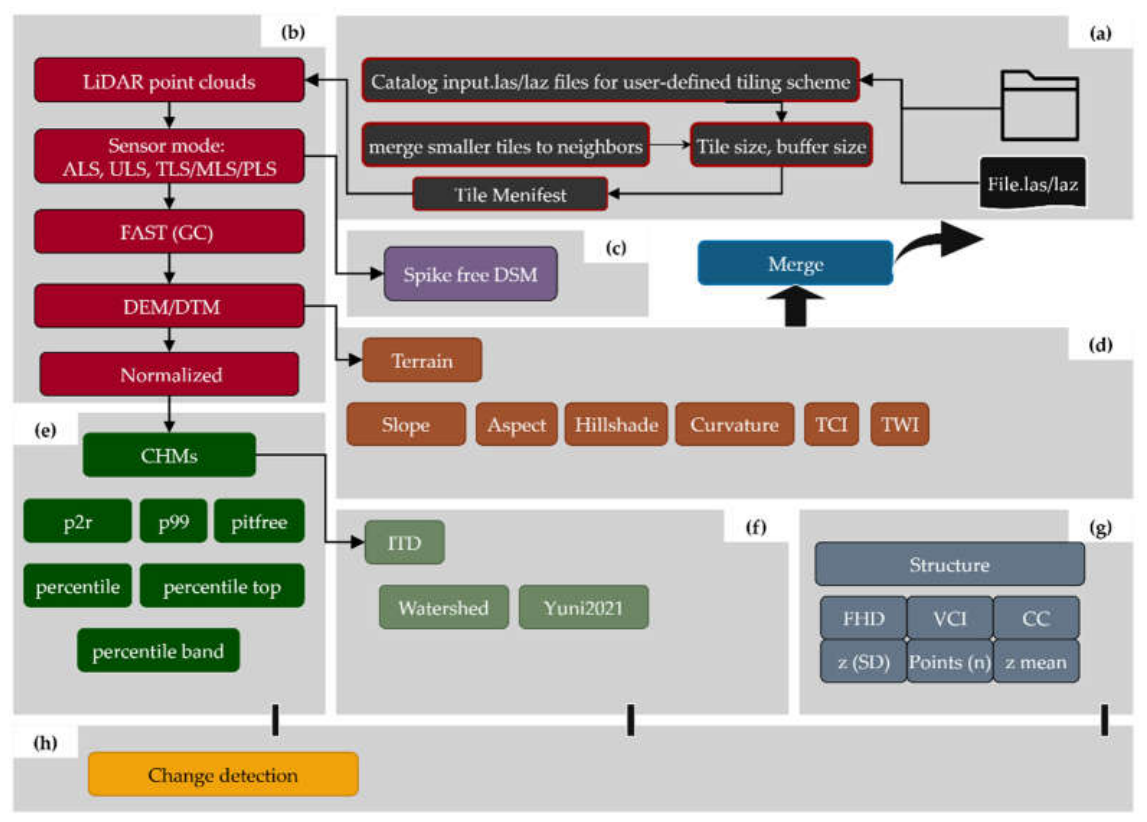
Figure 2.
Topographic and reference-classification characteristics of the five benchmark sites. For each site, the upper panel depicts terrain morphology and elevation variation, while the lower panel shows reference ground (red) and non-ground (green) returns. The sites span vegetation-dominated, mixed vegetation–terrain, and steep complex-terrain conditions.
Figure 2.
Topographic and reference-classification characteristics of the five benchmark sites. For each site, the upper panel depicts terrain morphology and elevation variation, while the lower panel shows reference ground (red) and non-ground (green) returns. The sites span vegetation-dominated, mixed vegetation–terrain, and steep complex-terrain conditions.
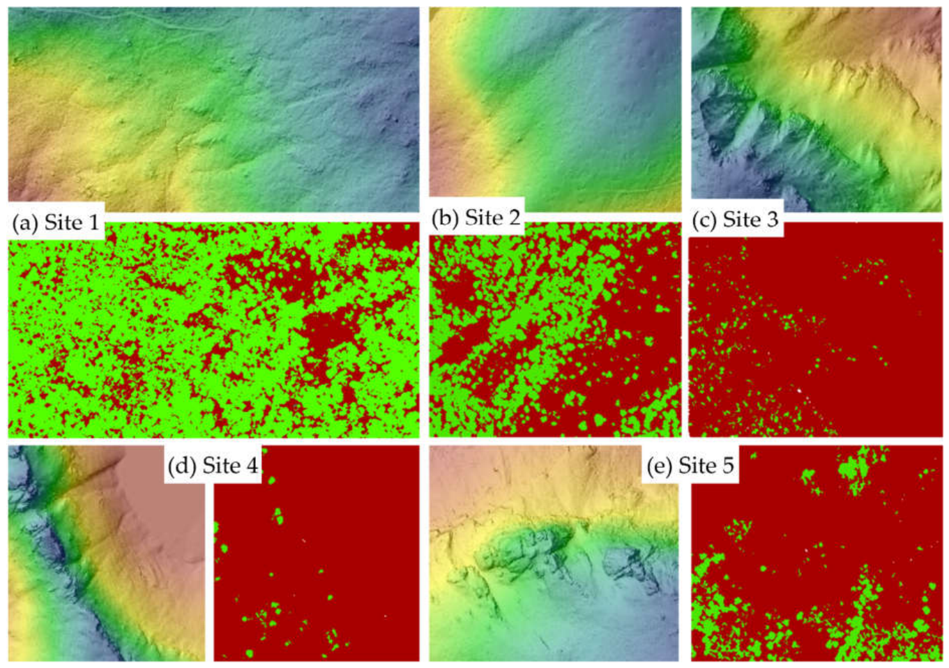
Figure 3.
Site-wise point-level ground-classification performance of FAST-GC, CSF, PTD, and PMF across the five controlled ALS benchmark sites. (a) F1-score, (b) intersection-over-union (IoU), (c) ground omission error (OE), and (d) normalized confusion behavior expressed as true-positive rate (TPR), true-negative rate (TNR), false-positive rate (FPR), and false-negative rate (FNR). Panels (a–c) illustrate changes in classification agreement and ground retention among sites, while panel (d) resolves the corresponding balance between correct ground retention and non-ground rejection.
Figure 3.
Site-wise point-level ground-classification performance of FAST-GC, CSF, PTD, and PMF across the five controlled ALS benchmark sites. (a) F1-score, (b) intersection-over-union (IoU), (c) ground omission error (OE), and (d) normalized confusion behavior expressed as true-positive rate (TPR), true-negative rate (TNR), false-positive rate (FPR), and false-negative rate (FNR). Panels (a–c) illustrate changes in classification agreement and ground retention among sites, while panel (d) resolves the corresponding balance between correct ground retention and non-ground rejection.
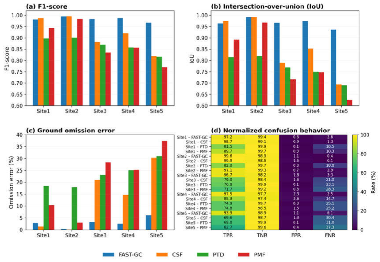
Figure 4.
Comparison of 0.5 m digital elevation models (DEMs) derived from ground points classified by FAST-GC, CSF, PTD, and PMF across benchmark Sites 2–5. DEM elevations are expressed as site-relative above-ground-level (AGL) values, with the minimum terrain elevation normalized to 0 m and a common elevation range applied across methods within each site. Red polygon boundaries delineate spatially contiguous regions where the absolute DEM difference from the reference terrain derived from the original ground class (class = 2) exceeds 0.25 m (|DoD| ≥ 0.25 m). Panels are arranged by site (rows) and ground-classification method (columns), enabling direct comparison of terrain-surface reconstruction and the spatial distribution of elevation discrepancies among methods. Site 1, similar to Site 2, is comparatively flat, with all algorithms having no significant errors, so it was not included in Figure 4.
Figure 4.
Comparison of 0.5 m digital elevation models (DEMs) derived from ground points classified by FAST-GC, CSF, PTD, and PMF across benchmark Sites 2–5. DEM elevations are expressed as site-relative above-ground-level (AGL) values, with the minimum terrain elevation normalized to 0 m and a common elevation range applied across methods within each site. Red polygon boundaries delineate spatially contiguous regions where the absolute DEM difference from the reference terrain derived from the original ground class (class = 2) exceeds 0.25 m (|DoD| ≥ 0.25 m). Panels are arranged by site (rows) and ground-classification method (columns), enabling direct comparison of terrain-surface reconstruction and the spatial distribution of elevation discrepancies among methods. Site 1, similar to Site 2, is comparatively flat, with all algorithms having no significant errors, so it was not included in Figure 4.
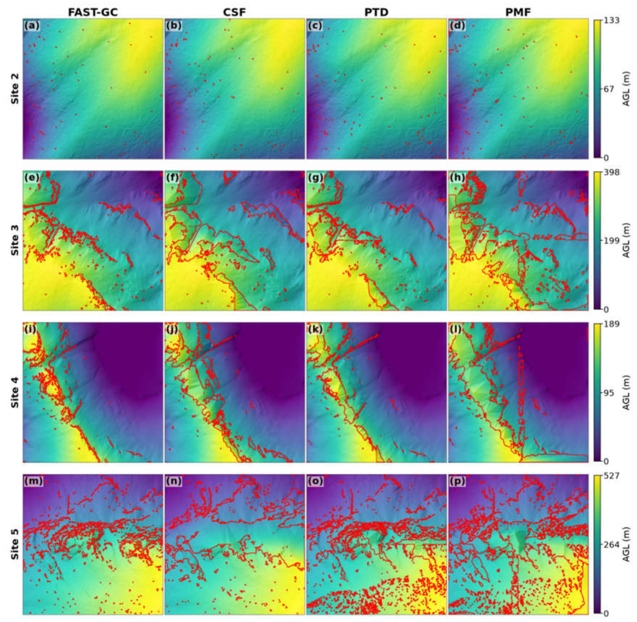
Figure 5.
DEM residuals as a function of reference terrain slope for (a) FAST-GC, (b) CSF, (c) PTD, and (d) PMF across benchmark Sites 2–5. Residuals were calculated as the method-derived 0.5 m DEM minus the reference DEM derived from the original ground class (class = 2) and grouped into 10° slope intervals from 0–10° to 80–90°. Points show the distribution of cell-level residuals within each slope class, while boxplots summarize their median and interquartile range. The horizontal dotted lines indicate the ±0.25 m DEM-difference threshold. Negative residuals indicate terrain underestimation relative to the reference DEM, whereas positive residuals indicate overestimation.
Figure 5.
DEM residuals as a function of reference terrain slope for (a) FAST-GC, (b) CSF, (c) PTD, and (d) PMF across benchmark Sites 2–5. Residuals were calculated as the method-derived 0.5 m DEM minus the reference DEM derived from the original ground class (class = 2) and grouped into 10° slope intervals from 0–10° to 80–90°. Points show the distribution of cell-level residuals within each slope class, while boxplots summarize their median and interquartile range. The horizontal dotted lines indicate the ±0.25 m DEM-difference threshold. Negative residuals indicate terrain underestimation relative to the reference DEM, whereas positive residuals indicate overestimation.
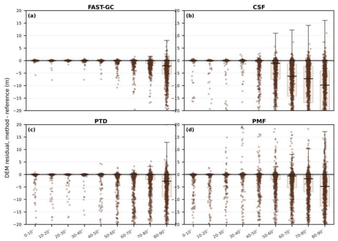
Figure 6.
Terrain-surface reconstruction error as a function of reference terrain slope for FAST-GC, CSF, PTD, and PMF across benchmark Sites 2–5. Cell-level DEM residuals from the 0.5 m method-derived and reference DEMs were pooled within 10° reference-slope intervals and summarized using (a) mean absolute error (MAE) and (b) root mean square error (RMSE). Increasing MAE and RMSE with slope indicates progressive loss of terrain-reconstruction accuracy, while the comparatively lower errors of FAST-GC at steeper slopes demonstrate greater preservation of complex terrain relative to the conventional filtering methods.
Figure 6.
Terrain-surface reconstruction error as a function of reference terrain slope for FAST-GC, CSF, PTD, and PMF across benchmark Sites 2–5. Cell-level DEM residuals from the 0.5 m method-derived and reference DEMs were pooled within 10° reference-slope intervals and summarized using (a) mean absolute error (MAE) and (b) root mean square error (RMSE). Increasing MAE and RMSE with slope indicates progressive loss of terrain-reconstruction accuracy, while the comparatively lower errors of FAST-GC at steeper slopes demonstrate greater preservation of complex terrain relative to the conventional filtering methods.
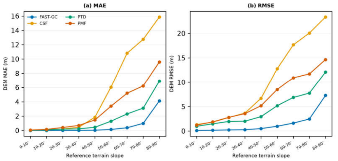
Figure 7.
Spatial variation in point density across the Jin benchmark sites (n=20) under the Original, D6, and D4 sampling conditions. (a) Distribution of ground and non-ground point densities calculated using a common 5 × 5 m grid. Boxplots represent the distributions of site-level median grid-cell densities, with individual points representing sites. (b) Site-wise spatial variation in total point density, expressed as the median and interquartile range (IQR) of 5 × 5 m grid-cell densities for each benchmark site.
Figure 7.
Spatial variation in point density across the Jin benchmark sites (n=20) under the Original, D6, and D4 sampling conditions. (a) Distribution of ground and non-ground point densities calculated using a common 5 × 5 m grid. Boxplots represent the distributions of site-level median grid-cell densities, with individual points representing sites. (b) Site-wise spatial variation in total point density, expressed as the median and interquartile range (IQR) of 5 × 5 m grid-cell densities for each benchmark site.
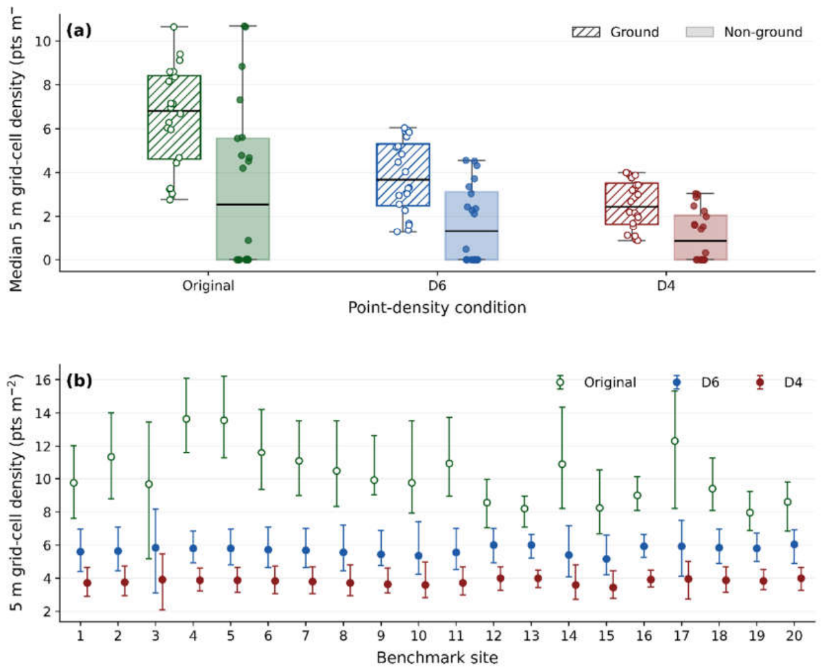
Figure 8.
Visual assessment of FAST-GC ground classification under reduced ALS point densities. FAST-GC classification results are shown for the same representative terrain profile after deterministic thinning to (a) D4 (~4 pts.m⁻²) and (b) D6 (~6 pts.m⁻²). Red points represent points classified as ground and green points represent non-ground returns (vegetation). Black circles identify representative locations that are enlarged in the corresponding insets to illustrate ground–non-ground separation beneath vegetation and across varying terrain.
Figure 8.
Visual assessment of FAST-GC ground classification under reduced ALS point densities. FAST-GC classification results are shown for the same representative terrain profile after deterministic thinning to (a) D4 (~4 pts.m⁻²) and (b) D6 (~6 pts.m⁻²). Red points represent points classified as ground and green points represent non-ground returns (vegetation). Black circles identify representative locations that are enlarged in the corresponding insets to illustrate ground–non-ground separation beneath vegetation and across varying terrain.
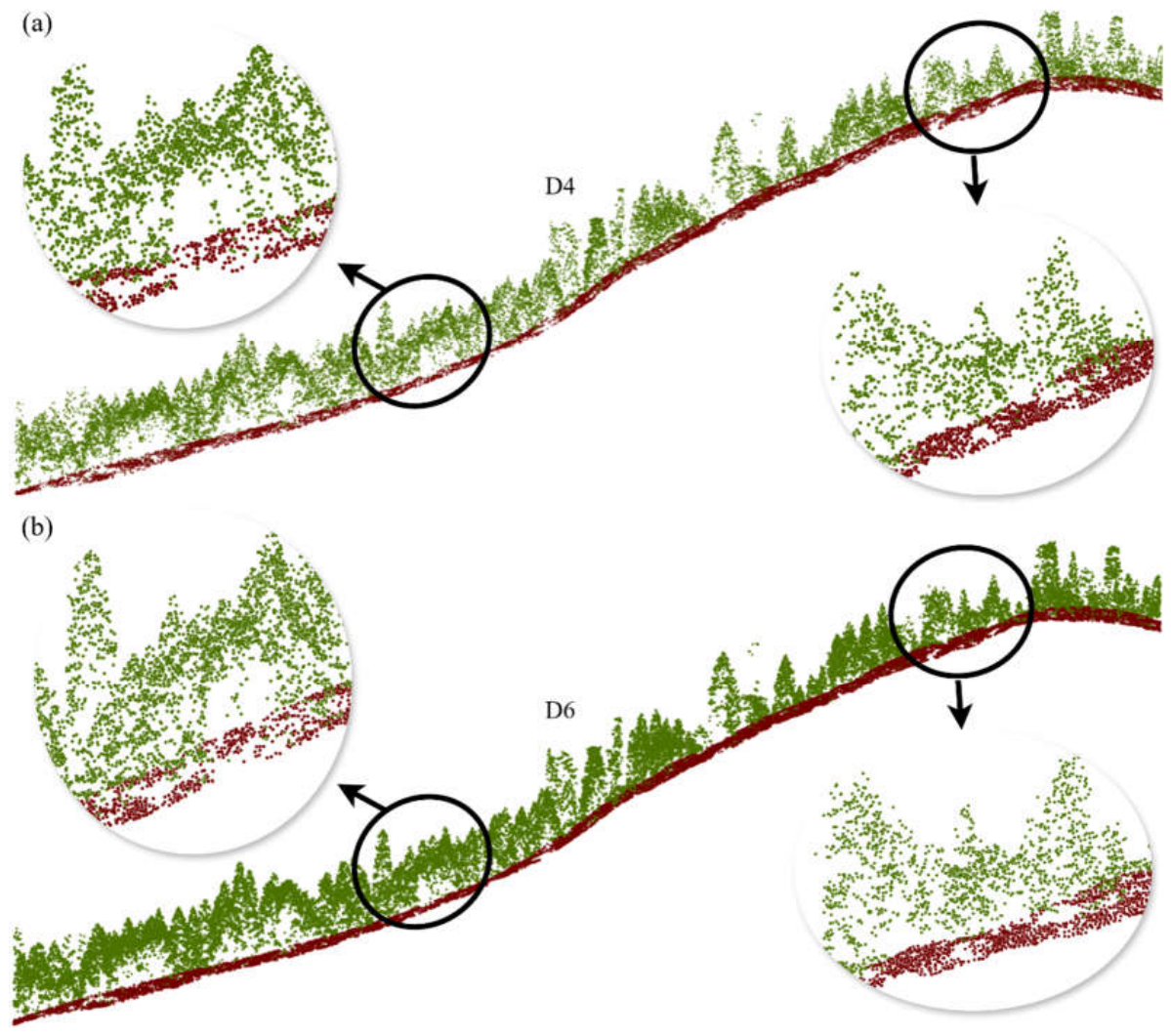
Figure 9.
Cross-platform consistency of 0.5 m DEMs derived from FAST-GC-classified ground points at BR01 (Germany, Site 8): (a) ULS leaf-off versus leaf-on, (b) ALS versus ULS leaf-off, (c) ALS versus ULS leaf-on, (d) ALS versus TLS, (e) TLS versus ULS leaf-off, and (f) TLS versus ULS leaf-on. Common comparison areas were 5.47 ha for ULS-based comparisons and 0.48 ha for comparisons involving TLS. Hexagonal bins show paired DEM observations, with the 1:1 relationship (red dashed line) and fitted regression (blue line).
Figure 9.
Cross-platform consistency of 0.5 m DEMs derived from FAST-GC-classified ground points at BR01 (Germany, Site 8): (a) ULS leaf-off versus leaf-on, (b) ALS versus ULS leaf-off, (c) ALS versus ULS leaf-on, (d) ALS versus TLS, (e) TLS versus ULS leaf-off, and (f) TLS versus ULS leaf-on. Common comparison areas were 5.47 ha for ULS-based comparisons and 0.48 ha for comparisons involving TLS. Hexagonal bins show paired DEM observations, with the 1:1 relationship (red dashed line) and fitted regression (blue line).
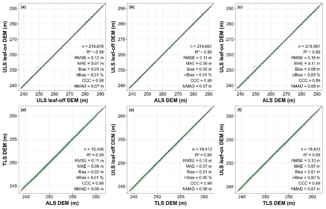
Figure 10.
Pairwise agreement among FAST-GC, PMF, CSF, and PTD classifications for the OpenGF mountainous scenes S7_3, S8_6, and S9_14. Cell values report positive agreement (%), with the corresponding Matthews correlation coefficient (MCC) and intersection over union (IoU). The final column reports the mean across the three scenes. The analysis is independent of the supplied OpenGF reference labels and therefore characterizes the degree to which independently applied ground-classification algorithms identify a common ground-point population.
Figure 10.
Pairwise agreement among FAST-GC, PMF, CSF, and PTD classifications for the OpenGF mountainous scenes S7_3, S8_6, and S9_14. Cell values report positive agreement (%), with the corresponding Matthews correlation coefficient (MCC) and intersection over union (IoU). The final column reports the mean across the three scenes. The analysis is independent of the supplied OpenGF reference labels and therefore characterizes the degree to which independently applied ground-classification algorithms identify a common ground-point population.
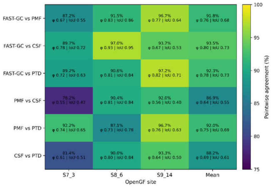
Figure 11.
Large-area stability assessment of FAST-GC across approximately 23 km² of heterogeneous forest at Lubrecht Experimental Forest, Montana, USA [64]. The upper panel presents the FAST-GC-derived high-resolution digital elevation model (HR-DEM) at 0.5 m spatial resolution, with representative locations (A–G) enlarged to illustrate terrain morphology across the processing extent. The subsets include channel-like and convergent terrain (A), rough local terrain beneath tall and heterogeneous canopy (B), irregular local relief (C), a localized depression-like feature (D), broader valley-and-ridge morphology with concave and convex hillslope forms (E), localized incised terrain (F), and narrow linear features consistent with unpaved roads or tracks (G). The lower panel presents the corresponding 0.5 m canopy height model (CHM) and the same enlarged locations, illustrating contrasting vegetation and canopy conditions overlying these terrain configurations. The spatially continuous HR-DEM and CHM, together with geographically distributed subsets A–G, illustrate large-area processing across heterogeneous canopy and terrain conditions without visually apparent systematic tile-boundary artifacts. The CHM was generated at the same 0.5 m spatial resolution using the pit-free algorithm implemented within the FAST-GC processing workflow (Figure 1).
Figure 11.
Large-area stability assessment of FAST-GC across approximately 23 km² of heterogeneous forest at Lubrecht Experimental Forest, Montana, USA [64]. The upper panel presents the FAST-GC-derived high-resolution digital elevation model (HR-DEM) at 0.5 m spatial resolution, with representative locations (A–G) enlarged to illustrate terrain morphology across the processing extent. The subsets include channel-like and convergent terrain (A), rough local terrain beneath tall and heterogeneous canopy (B), irregular local relief (C), a localized depression-like feature (D), broader valley-and-ridge morphology with concave and convex hillslope forms (E), localized incised terrain (F), and narrow linear features consistent with unpaved roads or tracks (G). The lower panel presents the corresponding 0.5 m canopy height model (CHM) and the same enlarged locations, illustrating contrasting vegetation and canopy conditions overlying these terrain configurations. The spatially continuous HR-DEM and CHM, together with geographically distributed subsets A–G, illustrate large-area processing across heterogeneous canopy and terrain conditions without visually apparent systematic tile-boundary artifacts. The CHM was generated at the same 0.5 m spatial resolution using the pit-free algorithm implemented within the FAST-GC processing workflow (Figure 1).
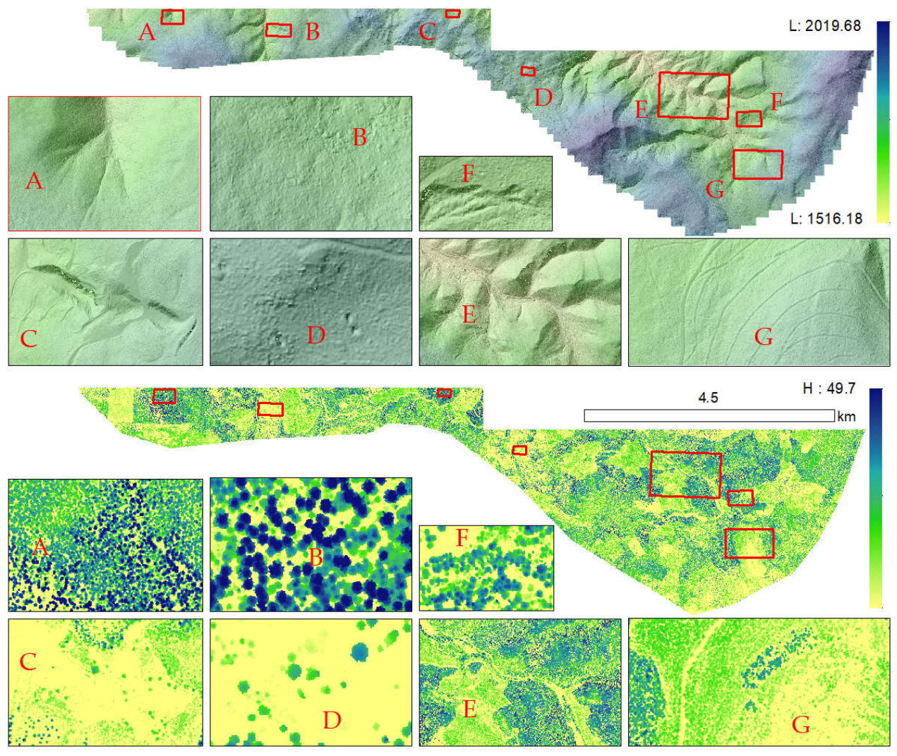

Table 1.
LiDAR datasets used for the evaluation of FAST-GC across contrasting sensor, vegetation, terrain, and sampling conditions. Dataset characteristics include sensor platform, spatial coverage, point density, reference ground/non-ground composition, elevation range, and the corresponding landscape or evaluation role. (N/A) Represent where information is not directly available from data sources.
Table 1.
LiDAR datasets used for the evaluation of FAST-GC across contrasting sensor, vegetation, terrain, and sampling conditions. Dataset characteristics include sensor platform, spatial coverage, point density, reference ground/non-ground composition, elevation range, and the corresponding landscape or evaluation role. (N/A) Represent where information is not directly available from data sources.
| Study area | Application | Location | Collection | Area (km2) | (pts m−2) | GC /N-GC (%) | Elevation range (m) | Canopy conditions |
| Site 1 | Benchmark | San Joaquin Range, CA, USA | ALS [17] | 0.50 | 11.82 | 40.36 / 59.64 | 1822.27–2020.75 | Dense forest; substantial canopy structure and locally steep terrain. |
| Site 2 | Courtwright Road, CA, USA | 0.25 | 10.30 | 69.09 / 30.91 | 2590.04–2752.96 | Moderately forested terrain; balanced vegetation–terrain challenge. | ||
| Site 3 | Wolverton–Tokopah, CA, USA | 0.25 | 8.49 | 96.86 / 3.14 | 2800.35–3217.89 | Sparse vegetation with steep, strongly varying topography. | ||
| Site 4 | 0.25 | 8.30 | 98.26 / 1.74 | 2904.96–3109.68 | Coupled vegetation and complex/steep terrain challenge. | |||
| Site 5 | 0.25 | 9.05 | 78.24 / 21.76 | 2175.60–2754.79 | Extreme relief and very steep terrain with moderate vegetation. | |||
| Site 6 | Cross-validation/Urban | Arnhem, Netherlands | ALS [60] | 0.50 | 18.57 | 42.17/57.83 | 7.20–38.76 | Urban site with substantial tree cover |
| Site 7 | Cross-validation | USA, New Zealand | ALS [59] | 0.75 | 16.16 | 14.28/85.72 | 83–883 | Mountain sites |
| Site 8 | Cross-platform validation | Germany | ALS/ULS/TLS [62] | ~0.12 | 72.5 (ALS) | N/A | 240-312 | Temperate mixed forest |
| Site 9 | Stability test | Lubrichat, USA | ALS [63] | 23 | 20.07 | N/A | 1516-2019 | Mountainous mixed-conifer forest |
Table 2.
Point-wise ground-truth classification performance of FAST-GC and three reference algorithms across the five controlled ALS benchmark sites.
Table 2.
Point-wise ground-truth classification performance of FAST-GC and three reference algorithms across the five controlled ALS benchmark sites.
| Site | Algorithm | Precision | Recall | F1 | IoU | MCC | CE (%) | OE (%) |
| Site1 |
FAST-GC | 0.99 | 0.97 | 0.98 | 0.96 | 0.96 | 0.85 | 2.87 |
| PTD | 0.99 | 0.82 | 0.90 | 0.81 | 0.85 | 0.10 | 18.46 | |
| CSF | 0.99 | 0.99 | 0.99 | 0.97 | 0.98 | 1.27 | 1.29 | |
| PMF | 0.99 | 0.90 | 0.94 | 0.89 | 0.91 | 0.52 | 10.33 | |
| Site2 |
FAST-GC | 0.99 | 0.996 | 0.99 | 0.991 | 0.98 | 0.47 | 0.41 |
| PTD | 0.99 | 0.82 | 0.90 | 0.82 | 0.76 | 0.15 | 17.96 | |
| CSF | 0.99 | 1.00 | 1.00 | 0.99 | 0.99 | 0.65 | 0.13 | |
| PMF | 0.99 | 0.97 | 0.98 | 0.97 | 0.95 | 0.30 | 2.93 | |
| Site3 |
FAST-GC | 0.99 | 0.96 | 0.98 | 0.96 | 0.65 | 0.06 | 3.81 |
| PTD | 0.99 | 0.77 | 0.87 | 0.77 | 0.31 | <0.01 | 23.12 | |
| CSF | 0.99 | 0.79 | 0.88 | 0.79 | 0.32 | 0.07 | 20.99 | |
| PMF | 1.00 | 0.72 | 0.83 | 0.72 | 0.27 | 0.04 | 28.32 | |
| Site4 |
FAST-GC | 1.00 | 0.97 | 0.985 | 0.97 | 0.59 | 0.04 | 2.89 |
| PTD | 1.00 | 0.75 | 0.86 | 0.75 | 0.22 | <0.01 | 25.07 | |
| CSF | 1.00 | 0.85 | 0.92 | 0.85 | 0.29 | 0.05 | 14.73 | |
| PMF | 1.00 | 0.75 | 0.86 | 0.75 | 0.22 | 0.03 | 25.18 | |
| Site5 |
FAST-GC | 0.99 | 0.93 | 0.96 | 0.92 | 0.85 | 0.33 | 6.82 |
| PTD | 0.99 | 0.69 | 0.82 | 0.69 | 0.57 | 0.04 | 31.00 | |
| CSF | 0.99 | 0.70 | 0.82 | 0.69 | 0.57 | 0.50 | 30.38 | |
| PMF | 0.99 | 0.63 | 0.77 | 0.63 | 0.51 | 0.19 | 37.35 | |
|
Macro-average |
FAST-GC | 0.99 | 0.966 | 0.98 | 0.96 | 0.81 | 0.35 | 3.36 |
| PTD | 0.99 | 0.77 | 0.87 | 0.77 | 0.54 | 0.06 | 23.12 | |
| CSF | 0.99 | 0.86 | 0.92 | 0.86 | 0.63 | 0.51 | 13.50 | |
| PMF | 0.99 | 0.79 | 0.88 | 0.79 | 0.57 | 0.22 | 20.82 |
Notes: Precision, Recall, F1, IoU, and MCC are reported as proportions rounded to two decimal places; CE and OE are percentages. Bold values indicate the best result within each stress-test site for the corresponding metric. Best-performing methods were identified from the unrounded results.
Table 3.
Point-wise classification performance of FAST-GC, PTD, CSF, and PMF on the urban and extreme-topography ALS stress-test sites.
Table 3.
Point-wise classification performance of FAST-GC, PTD, CSF, and PMF on the urban and extreme-topography ALS stress-test sites.
| Test | Method | Precision | Recall | F1 | IoU | MCC | CE (%) | OE (%) |
| Urban (Site 6) | FAST-GC | 0.86 | 0.99 | 0.92 | 0.86 | 0.87 | 13.17 | 0.27 |
| PTD | 0.95 | 0.84 | 0.89 | 0.81 | 0.83 | 4.72 | 15.92 | |
| CSF | 0.91 | 1.00 | 0.95 | 0.91 | 0.92 | 9.21 | 0.12 | |
| PMF | 0.78 | 1.00 | 0.87 | 0.78 | 0.78 | 22.45 | <0.01 |
Table 4.
Point-wise FAST-GC classification performance across the 20 benchmark sites at original point density. Ground was treated as the positive class. CE, commission error; OE, omission error. N/A indicates that MCC is undefined for Site 20 because this bare-earth site contains no reference non-ground points. Macro-averages use all 20 sites for defined metrics; MCC is averaged across the 19 sites for which it is defined. Displayed values are truncated to two decimal places (not rounded).
Table 4.
Point-wise FAST-GC classification performance across the 20 benchmark sites at original point density. Ground was treated as the positive class. CE, commission error; OE, omission error. N/A indicates that MCC is undefined for Site 20 because this bare-earth site contains no reference non-ground points. Macro-averages use all 20 sites for defined metrics; MCC is averaged across the 19 sites for which it is defined. Displayed values are truncated to two decimal places (not rounded).
| Site | Precision | Recall | F1 | IoU | MCC | CE (%) | OE (%) |
| Site 1 | 0.99 | 0.99 | 0.99 | 0.99 | 0.98 | 0.47 | 0.41 |
| Site 2 | 0.99 | 0.98 | 0.98 | 0.97 | 0.97 | 0.81 | 1.42 |
| Site 3 | 0.98 | 0.93 | 0.95 | 0.92 | 0.93 | 1.43 | 6.59 |
| Site 4 | 0.98 | 0.91 | 0.94 | 0.90 | 0.93 | 1.87 | 8.41 |
| Site 5 | 0.95 | 0.93 | 0.94 | 0.89 | 0.92 | 4.15 | 6.66 |
| Site 6 | 0.99 | 0.95 | 0.97 | 0.95 | 0.96 | 0.33 | 4.38 |
| Site 7 | 0.98 | 0.96 | 0.97 | 0.95 | 0.95 | 1.98 | 3.05 |
| Site 8 | 0.98 | 0.98 | 0.98 | 0.96 | 0.96 | 1.18 | 1.85 |
| Site 9 | 0.99 | 0.98 | 0.99 | 0.98 | 0.96 | 0.64 | 1.23 |
| Site 10 | 0.98 | 0.96 | 0.97 | 0.94 | 0.95 | 1.54 | 3.58 |
| Site 11 | 0.98 | 0.98 | 0.98 | 0.96 | 0.96 | 1.98 | 1.47 |
| Site 12 | 0.99 | 0.96 | 0.98 | 0.96 | 0.65 | 0.06 | 3.80 |
| Site 13 | 0.99 | 0.97 | 0.98 | 0.97 | 0.59 | 0.04 | 2.89 |
| Site 14 | 0.98 | 0.92 | 0.95 | 0.91 | 0.91 | 1.24 | 7.12 |
| Site 15 | 0.99 | 0.93 | 0.96 | 0.92 | 0.85 | 0.33 | 6.82 |
| Site 16 | 0.99 | 0.93 | 0.96 | 0.93 | 0.72 | 0.28 | 6.56 |
| Site 17 | 0.99 | 0.94 | 0.97 | 0.94 | 0.80 | 0.26 | 5.42 |
| Site 18 | 0.99 | 0.96 | 0.98 | 0.96 | 0.16 | 0.00 | 3.67 |
| Site 19 | 0.99 | 0.98 | 0.98 | 0.97 | 0.94 | 0.50 | 1.53 |
| Site 20 | 1.00 | 0.99 | 0.99 | 0.99 | N/A | 0.00 | 0.98 |
| Macro-average | 0.99 | 0.96 | 0.97 | 0.95 | 0.85 | 0.95 | 3.89 |
Table 5.
Point-wise FAST-GC performance under point-density reduction across the 20 benchmark sites. Values are site-level macro-averages. Balanced Accuracy (BA), commission error (CE), omission error (OE). Original denotes the unthinned point cloud; D6 (6 pts./m²) and D4 (4 pts./m²) denote the reduced-density datasets. Displayed values are truncated to two decimal places (not rounded).
Table 5.
Point-wise FAST-GC performance under point-density reduction across the 20 benchmark sites. Values are site-level macro-averages. Balanced Accuracy (BA), commission error (CE), omission error (OE). Original denotes the unthinned point cloud; D6 (6 pts./m²) and D4 (4 pts./m²) denote the reduced-density datasets. Displayed values are truncated to two decimal places (not rounded).
| Point density | Precision | Recall | F1 | IoU | MCC | CE | OE (%) | BA |
| Original | 0.99 | 0.96 | 0.97 | 0.95 | 0.85 | 0.95 | 3.89 | 0.97 |
| D6 | 0.98 | 0.96 | 0.97 | 0.95 | 0.85 | 1.15 | 3.28 | 0.97 |
| D4 | 0.98 | 0.96 | 0.97 | 0.95 | 0.85 | 1.24 | 3.24 | 0.97 |
Table 6.
FAST-GC DEM (0.5 m) accuracy under point-density reduction across the 20 benchmark sites. Values are macro-averages across the 20 benchmark sites. mean absolute error (MAE); root mean square error (RMSE); P95 absolute error, 95th percentile of absolute DEM error. Bias is FAST-GC DEM minus reference DEM. Displayed values are truncated to two decimal places (not rounded).
Table 6.
FAST-GC DEM (0.5 m) accuracy under point-density reduction across the 20 benchmark sites. Values are macro-averages across the 20 benchmark sites. mean absolute error (MAE); root mean square error (RMSE); P95 absolute error, 95th percentile of absolute DEM error. Bias is FAST-GC DEM minus reference DEM. Displayed values are truncated to two decimal places (not rounded).
| Point density | Bias (m) | MAE (m) | RMSE (m) | P95 absolute error (m) |
| Original | -0.04 | 0.07 | 0.38 | 0.29 |
| D6 | -0.04 | 0.09 | 0.39 | 0.34 |
| D4 | -0.04 | 0.11 | 0.42 | 0.40 |
Table 7.
Point-wise agreement of FAST-GC, PMF, CSF, and PTD with OpenGF for three mountainous scenes (S7_3, S8_6, and S9_14). Metrics include precision, recall, F1-score, intersection over union (IoU), Matthews correlation coefficient (MCC), commission error (CE), omission error (OE), and balanced accuracy (BA). CE and OE are relative to the supplied OpenGF reference labels. Bold values indicate the best performance for each metric.
Table 7.
Point-wise agreement of FAST-GC, PMF, CSF, and PTD with OpenGF for three mountainous scenes (S7_3, S8_6, and S9_14). Metrics include precision, recall, F1-score, intersection over union (IoU), Matthews correlation coefficient (MCC), commission error (CE), omission error (OE), and balanced accuracy (BA). CE and OE are relative to the supplied OpenGF reference labels. Bold values indicate the best performance for each metric.
| Site | Algorithm | Precision | Recall | F1 | IoU | MCC | CE (%) | OE (%) | BA |
| S7_3 | FAST-GC | 0.43 | 0.98 | 0.59 | 0.42 | 0.58 | 56.84 | 1.87 | 0.89 |
| S7_3 | PMF | 0.66 | 0.89 | 0.76 | 0.61 | 0.73 | 33.44 | 10.78 | 0.91 |
| S7_3 | CSF | 0.32 | 0.96 | 0.48 | 0.31 | 0.46 | 67.79 | 3.29 | 0.83 |
| S7_3 | PTD | 0.58 | 0.94 | 0.72 | 0.57 | 0.70 | 41.09 | 5.15 | 0.92 |
| S8_6 | FAST-GC | 0.73 | 0.99 | 0.84 | 0.72 | 0.70 | 26.94 | 0.64 | 0.84 |
| S8_6 | PMF | 0.78 | 0.93 | 0.85 | 0.74 | 0.71 | 21.90 | 6.43 | 0.86 |
| S8_6 | CSF | 0.71 | 0.99 | 0.83 | 0.71 | 0.68 | 28.61 | 0.68 | 0.83 |
| S8_6 | PTD | 0.74 | 0.89 | 0.81 | 0.68 | 0.64 | 25.15 | 10.36 | 0.82 |
| S9_14 | FAST-GC | 0.43 | 0.94 | 0.59 | 0.42 | 0.61 | 56.81 | 5.44 | 0.94 |
| S9_14 | PMF | 0.51 | 0.84 | 0.63 | 0.46 | 0.63 | 48.91 | 15.58 | 0.90 |
| S9_14 | CSF | 0.25 | 0.79 | 0.38 | 0.24 | 0.41 | 74.30 | 20.55 | 0.84 |
| S9_14 | PTD | 0.45 | 0.93 | 0.61 | 0.44 | 0.63 | 54.37 | 6.07 | 0.94 |
| Mean | FAST-GC | 0.53 | 0.97 | 0.67 | 0.52 | 0.63 | 46.86 | 2.65 | 0.89 |
| Mean | PMF | 0.65 | 0.89 | 0.75 | 0.60 | 0.69 | 34.75 | 10.93 | 0.89 |
| Mean | CSF | 0.43 | 0.91 | 0.56 | 0.42 | 0.52 | 56.90 | 8.17 | 0.84 |
| Mean | PTD | 0.59 | 0.92 | 0.71 | 0.56 | 0.66 | 40.21 | 7.20 | 0.89 |
Disclaimer/Publisher’s Note: The statements, opinions and data contained in all publications are solely those of the individual author(s) and contributor(s) and not of MDPI and/or the editor(s). MDPI and/or the editor(s) disclaim responsibility for any injury to people or property resulting from any ideas, methods, instructions or products referred to in the content. |
© 2026 by the authors. Licensee MDPI, Basel, Switzerland. This article is an open access article distributed under the terms and conditions of the Creative Commons Attribution (CC BY) license.
Copyright: This open access article is published under a Creative Commons CC BY 4.0 license, which permit the free download, distribution, and reuse, provided that the author and preprint are cited in any reuse.