

Submitted:
18 September 2026
Posted:
20 September 2026
You are already at the latest version
Abstract
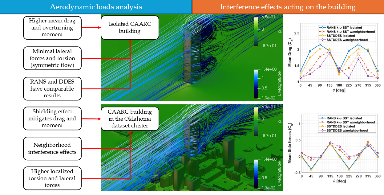
Urban densification and high-rise buildings alter local wind flows, thereby affecting structural aerodynamic loads. To address this issue, the present numerical study investigates the insertion of a standard high-rise building within the Oklahoma City urban dataset. Computational Fluid Dynamics simulations were conducted across eight wind incidence angles (from 0° to 360° at 45° intervals) using two turbulence models, the Reynolds-Averaged Navier-Stokes (RANS) with k-ω Shear Stress Transport closure equations and the hybrid approach Shear Stress Transport Delayed Detached-Eddy Simulations (SSTDDES). A numerical validation was conducted using the Michelstadt experimental dataset, showing that both turbulence models achieved satisfactory statistical agreement with wind tunnel data. Structural forces were quantified using aerodynamic coefficients, and the results demonstrate that while the surrounding neighborhood provides a shielding effect, it simultaneously induces complex wakes that amplify localized peak lateral forces and torsion. Notably, the SSTDDES model captured higher peak structural loads and gusts compared to the RANS approach, concluding that domain-averaged criteria can obscure severe localized hazards, emphasizing that safe high-density developments require adequate turbulence models and site-specific aerodynamic investigations.
Keywords:
computational fluid dynamics
; RANS
; DES
; wind loads
; high-rise buildings
1. Introduction
Urbanization and technological advances in construction have transformed cities worldwide, increasing population density and promoting the “vertical city” concept through the proliferation of skyscrapers. This evolution has become a major concern in engineering design, as highlighted by Caswell et al. [1], who demonstrated the influence of urban geometry on thermal and visual comfort in high-rise districts. Beyond representing economic development, tall buildings also optimize land use and encourage public transportation in dense urban centers [2]. Nevertheless, increasing building heights and urban densification affect the urban environment by modifying wind flow patterns and pollutant dispersion, while also influencing thermal comfort, urban energy efficiency and intensifying urban heat island effects, as reported by Siddique et al. [3].
The Atmospheric Boundary Layer (ABL) constitutes the region adjacent to the Earth’s surface where the flow is directly influenced by surface friction, thermal stratification resulting from solar radiation, and the planet’s rotational effects, whereas within cities, research specifically addresses the Urban Canopy Layer (UCL), which extends from the ground level to a region immediately above the building tops, thereby encompassing the zone of influence characterized by flow separation and the formation of turbulent wakes. The differences between the ABL and the UCL, along the three primary flow regions are illustrated in Figure 1.
According to Chen et al. [4], ventilation within the UCL plays a key role in pollutant dispersion and thermal regulation, being influenced by geometric aspect ratios, packing density, and wind direction. These factors also drive incoming turbulence and aerodynamic interference, modifying the wind loads acting on building facades. Therefore, Wind Engineering in urban environments requires a multidisciplinary approach that accounts for the strong interaction between geometric and aerodynamic parameters.
The assessment for Wind Engineering studies necessitates the application of specific methodologies, which can be broadly classified into three primary approaches:
- Physical testing in reduced-scale wind tunnels allow complex aerodynamic effects to be reproduced under controlled laboratory conditions but it limited by relatively high costs [7].
- Numerical simulations via Computational Fluid Dynamics (CFD), which offer operational flexibility, but their predictive accuracy remains dependent on the appropriate selection of turbulence models, the experimental validation of numerical results, and available High-Performance Computing (HPC) resources [7,8].
CFD modeling has consolidated as a tool for investigating urbanization effects on natural ventilation, atmospheric flow and wind-induced actions on structures, employing diverse approaches that range from simplified models with idealized geometries and urban canyons to simulations of complex and expansive urban areas:
- Hui et al. [9] investigated the influences of trees planted on building facades on the aerodynamics of tall buildings using Large-Eddy Simulations (LES) turbulence model, finding out that vegetation compresses the separation bubble and reduces mean and fluctuating pressures on the side walls, concluding that planting trees on balconies attenuates lift fluctuations and reduces wind loads on the building.
- Silva et al. [10] assessed Pedestrian Wind Comfort (PWC) within an array of nine buildings characterized by variations in height and wind incidence angle using the Reynolds-Averaged Navier-Stokes (RANS) model with the classic formulation, finding that wind configurations aligned with the canyons generate dangerous velocities, whereas oblique angles mitigate peak values.
- Villalobos-García et al. [11] investigated the effects of surrounding structures on the wind loads acting upon a high-rise building using a RANS model with the Shear Stress Transport (SST) formulation, finding that nearby configurations reduce global pressure coefficients by an average of 27% but generate localized suction fields on windward faces.
- Ibarra-Hernández et al. [12] investigated turbulent flow patterns within a real low-rise urban landscape in Monterrey (Mexico) using the RANS model with the Renormalization Group (RNG) closure equations, finding that mean velocity fields remain independent of the Reynolds number and, consequently, their evaluation demonstrates that main avenues concentrate high velocities and promote turbulence generation.
The selection of the modeling strategy depends on the equilibrium between representative fidelity and computational feasibility, given that large-scale urban simulations can demand meshes with a large number of cells, which renders the utilization of conventional computational resources unfeasible [13].
CFD simulations enable the evaluation of parameters related to wind comfort and safety, provided that appropriate turbulence models and boundary conditions are implemented. While Large-Eddy Simulations (LES) models exhibit high capability in reproducing complex urban flows, hybrid approaches such as Detached-Eddy Simulations (DES) combine the advantages of RANS and LES formulations, providing improved predictions of boundary layer separation, vortex formation and aerodynamic forces [14]. In Brazil, the evaluation of wind effects is based on the Associação Brasileira de Normas Técnicas (ABNT) NBR 6123/2023 [15] standard code, yet CFD has consolidated as an alternative capable of estimating aerodynamic pressures and forces with accuracy comparable to wind tunnel testing, while offering enhanced flexibility and lower costs.
This work is organized as follows: Section 2 presents a review of the literature concerning aerodynamic forces and turbulence modeling. Section 3 describes the adopted methodology, including the main equations, turbulence models, numerical methods, computational domain, boundary conditions and mesh discretization procedure. Section 4 provides numerical validation through the Michelstadt urban neighborhood benchmark, where the predicted velocity fields obtained with different turbulence models and numerical schemes are compared against the experimental data. Section 5 presents and discusses the aerodynamic coefficients for the investigated urban configuration with the two analyzed turbulence models. Finally, Section 6 summarizes the main conclusions, highlighting the limitations of the present study, and outlines recommendations for future research.
2. Literature Review
Property transport within a fluid, including momentum, heat and scalar concentrations, occurs via convection associated with the mean velocity field and through diffusion of either molecular or turbulent nature, whereas turbulence itself is characterized by chaotic, three-dimensional, and unsteady motions that constitute a property of the flow rather than the fluid. The flow regime is determined by the Reynolds number:
where , and are, respectively, the fluid specific mass, velocity and dynamic viscosity and is the characteristic length. Generally, for internal flows in pipes or ducts, particularly circular ones, values below 2300 indicate laminar flow, meaning it is predominantly laminar with perturbations damped by viscosity, whereas for values greater than 4000, the flow becomes turbulent, leading to perturbation amplification and multi-scale vortex formation. In this turbulent regime, the elevated diffusivity enhances the transport of mass, momentum and energy, while Turbulent Kinetic Energy (TKE) is transferred from large to small scales through the energy cascade process until it is dissipated into heat by molecular viscosity.
2.1. Turbulence Modelling
CFD provides a numerical approach to simulate fluid flow, heat transfer, and related phenomena through the resolution of equations of motion. In urban applications, this field has expanded the comprehension of flow patterns across complex geometries while overcoming limitations inherent to experimental techniques [14]. Its engineering applications encompass the assessment of wind potential, pollutant dispersion, urban microclimates, pedestrian comfort, and wind-induced loads on structures. Each of these areas presents challenges related to geometric complexity, multiscale interactions, and turbulence generation induced by buildings, vegetation, and topography, thereby rendering turbulence modeling an important aspect for simulation accuracy.
The primary turbulence strategies are categorized into: (i) RANS formulations, which are grounded in the time-averaging of flow equations; (ii) LES, which explicitly resolve large-scale vortices while modeling sub-grid scales; and (iii) hybrid frameworks, such as DES, which combine RANS formulations in near-wall regions with LES treatments in detached flow zones to achieve an equilibrium between computational cost and physical fidelity. Each modeling approach involves a direct trade-off between predictive accuracy and computational resource allocation, such that RANS formulations remain the most widely implemented in engineering practices due to their computational efficiency and capacity to adequately represent mean flow characteristics, although they depend on closure equations to account for turbulent transport effects [16]. The main closure models are based on the and formulations, which differ with respect to their transport equations, treatment of turbulence anisotropy, and near-wall effect modeling [17,18,19].
The RANS equations describe turbulent flows through the Reynolds decomposition, which separates each instantaneous quantity into a mean and a fluctuating component [20], a formulation that introduces the Reynolds stresses responsible for the closure problem and consequently requires additional equations to represent their transport effects:
where are the mean velocity components, are the cartesian coordinates, are the mean body forces, is the mean pressure, is the Kronecker delta, and are the Reynolds stresses. For Wind Engineering purposes, is adopted as 1.225 kg/m³, representing air density at 15 °C at sea level [21].
Among these additional equations, the SST scheme combines the advantages of the standard and formulations [22,23] by solving two transport equations: one for the TKE () and another for the specific dissipation rate ():
where represents the material derivative operator represents both local temporal variation and convective transport, denotes the kinematic viscosity, is the turbulent kinematic viscosity, is the invariant of the fluid strain rate tensor, is the TKE production term arising from mean velocity gradient shear, and represent the effective diffusivity coefficients for TKE and specific dissipation, respectively, is a cross-diffusion term enabling the transition between and formulations, and and are additional source terms. The empirical constants , and serve model closure and calibration purposes, whereas and function as blending factors. The kinematic turbulent viscosity is formulated to limit shear stresses according to:
where and are empirical constants and is a blending function. This formulation enables to limit shear stresses and to improve predictive capabilities in regions exhibiting adverse pressure gradients.
The DES formulation combines the advantages of RANS and LES models within a unified approach, implementing RANS in near-wall regions and LES in separated flow zones [24], a transition achieved by replacing the wall distance with a modified length scale:
Which is dependent on grid cell dimensions. is a calibration constant and denotes the maximum dimension of the mesh cell, a modification that causes the model to behave as a RANS near solid boundaries () and analogously to a Smagorinsky LES model in far-field regions, thereby making scale dependency a local property.
The original DES formulation can exhibit premature transition to LES mode when excessive grid refinement occurs within the boundary layer, artificially reducing turbulent viscosity and inducing spurious flow separation. To overcome this limitation, the Delayed Detached-Eddy Simulations (DDES) variant was developed by Spalart et al. [25], introducing a shielding function to preserve RANS behavior across wall-bounded attached flow regions.
Among these variants, the Shear Stress Transport Delayed Detached-Eddy Simulations (SSTDDES) model stands out by utilizing the turbulence length scale of the SST model to govern the transition between RANS and LES modes, providing enhanced predictive fidelity for vortex shedding and separated flows at lower computational cost than full LES simulations [26].
The LES formulation in far-field regions relies on Kolmogorov’s similarity theory [27], according to which large-scale vortices depend directly on flow geometry, whereas smaller scales exhibit universal isotropic behavior. Consequently, LES explicitly resolves large turbulent structures while modeling only sub-grid scales via a Sub-Grid Scale (SGS) model. The scale separation is executed through a spatial filtering operation, computationally represented by the grid resolution itself, yielding the filtered mass and momentum conservation equations:
where are the filtered velocity components, and is the sub-grid stress tensor, which arises to introduce the closure problem. In the adopted SSTDDES formulation, the SGS stress tensor is modeled by the Smagorinsky scheme [28].
2.2. Wind Effects in Urban Engineering
Wind actions induce loads on tall and slender buildings, since they are driven by asymmetric pressure distributions resulting from geometry, different wind incidence angles, and surrounding aerodynamic interference effects, rendering the analysis of aerodynamic and aeroelastic effects essential, particularly regarding transverse and torsional forces that frequently determine structural dimensioning and serviceability criteria [29].
Design standards differ in their definitions of basic wind velocity and implemented correction factors, given that while the Brazilian ABNT NBR 6123 [15] and American ASCE 7-22 [30] standards utilize a 3-second gust velocity, Eurocode 1 [31] considers a 10-minute mean velocity and the Chinese GB 50009/2012 [32] code employs specific reference pressure and height parameters. Nevertheless, despite these distinct methodological approaches, prescriptive codes can be insufficient for high-rise buildings or complex geometries, thereby necessitating complementary evaluation via wind tunnel testing or CFD frameworks.
Within urban regions, surrounding buildings modify the flow field and consequently wind-induced actions, where despite the introduction of neighborhood coefficients by the standard codes [15,30,31,32], its application remains limited to prescriptive estimates that do not adequately account for complex flows or pedestrian comfort parameters, thereby requiring specific investigations that evaluate the influence of urban geometry, relative building placement, and wind incidence angles [33]. According to Blessmann [34], the primary interference phenomena encompass buffeting, which is induced by periodic vortex shedding mechanisms; the Venturi effect, responsible for flow acceleration between adjacent structures; and wake turbulence, which alters the wind loads acting upon downstream configurations through recirculation regions and vortex formation.
CFD has consolidated as a tool for building aerodynamics analysis, being implemented in the evaluation of wind loads, natural ventilation, urban microclimates, and the optimization of urban layouts for energy efficiency [35], while additionally enabling the investigation of urban geometry influence on flow patterns and pedestrian safety [36]. To guarantee the reliability of the numerical results, the implementation of best practices guidelines is required. These include adequate mesh resolution, the appropriate selection of the turbulence model, and the systematic validation of numerical data against experimental benchmarks.
3. Methodology
This section details the methodology, which encompasses the evaluation of aerodynamic coefficients and their computational formulation within OpenFOAM, the simulation domain, boundary conditions, near-wall treatments, and the implemented numerical schemes. All simulations were carried out in OpenFOAM v2206, using HPC resources from Centro Nacional de Desempenho de Alto Desempenho em São Paulo (CENAPAD-SP) at Universidade Estadual de Campinas (UNICAMP). The specific HPC resources employed for the simulations consisted of two AMD EPYC 7662 processors based on the Zen 2 architecture, each featuring 64 cores, for a total of 128 cores, with 512 GB of available RAM and 328 TFLOPS distributed across 58 compute nodes. Since each simulation utilizes a single compute node, approximately 5.65 TFLOPS are employed for each case.
3.1. Aerodynamic Coefficients
The quantification of wind forces on buildings is performed through aerodynamic coefficients, which represent dimensionless parameters relating forces and moments to flow properties and structural geometry. The mean pressure coefficient describes the surface pressure relative to the freestream static and dynamic pressures , according to:
where = 0 Pa and = 1 m/s are, respectively, the reference pressure and velocity of the undisturbed freestream flow.
Integrating these pressure coefficients over the surface of the main building yields the overall aerodynamic forces and moments acting on the building:
where and are, respectively, the normal pressure and the tangential viscous forces, is the face area vector, and corresponds to the deviatoric stress tensor. These quantities are expressed as the drag (), side (), and lift () forces, as torsional () and overturning ( and ) moments:
where , and represent the reference areas (where the normal area to the force direction is considered), and or donates the reference length associated with the rotational axis of the moment, as illustrated by Figure 2 showing the effects of all these coefficients on a representative building, in which , and correspond to depth, width and height dimensions, respectively.
3.2. Simulation Domain
The computational domain and boundary conditions were defined based on the works of Aboshosha et al. [37], Elshaer et al. [38,39], and Liu et al. [40], adopting dimensions of 20×10×6, with the building arrangement positioned at 5 from the inlet, 15 from the outlet, 5 from the lateral boundaries, and 6 from the top boundary, adhering to the best practices guidelines for CFD simulations in urban environments proposed by Franke et al. [41] and Tominaga et al. [42]. Figure 3 shows a perspective view of this computational domain.
The mesh is generated through a two-step process, wherein the blockMesh utility initially builds the background mesh with progressive refinement toward the building region to concentrate elements near the model and ground, followed by snappyHexMesh, which executes local refinement and geometric fitting via castellation and snapping stages.
The building arrangement selected for this study corresponds to the Oklahoma City (USA) downtown cluster dataset provided by the University of Hamburg (Germany) through the European Cooperation in Science and Technology (COST) framework [43]. The selection of this specific urban arrangement is primarily justified by its adoption as a benchmark model in urban aerodynamics and microclimate studies, since high-fidelity three-dimensional geometric datasets of real cities are often proprietary or require costly topographical surveys. The model features an open space between structures near the central location, where two distinct scenarios are evaluated regarding the aerodynamic analysis: the isolated configuration, and the insertion in a previously empty space of the Commonwealth Advisory Aeronautical Research Council (CAARC) ( = 45.72 m; = 30.48 m; = 182.88 m) standard tall building model [44]. Figure 4 details the mesh condition in the model before and after the insertion of the high-rise structure. This comparison aims to identify how aerodynamic coefficients and, consequently, the structural performance of a high-rise building are influenced by neighborhood interference effects across different wind incidence angles.
3.3. Boundary Conditions
For the RANS SST model, the boundary conditions were specified to reproduce a neutral ABL, in accordance with Hargreaves and Wright [45], Yang et al. [46], and Richards and Norris [47]. The friction velocity is calculated by:
Where = 0.41 is the von Kárman constant, is the height above ground level and = 0.03 m is the atmospheric roughness parameter [48]. The logarithmic profile along with the distributions of TKE () and specific dissipation rate () are defined by:
Where = 0.09, and are empirical constants to adjust the functions to the logarithmic profile. At the inlet, velocity is prescribed as Eq. (19), is set to 0.00375 m²/s², = 0.061 s-1 and is fixed as zero. At the outlet, zero-gradient conditions are imposed on velocity and transport variables, while pressure is fixed at zero. The top and lateral boundaries are modeled as symmetry planes, thereby eliminating blockage effects and the development of artificial boundary layers.
For the SSTDDES model, the steady-state solution obtained from the RANS simulation serves as the initial condition, maintaining identical boundary conditions for scalar transport quantities. The distinction lies in replacing the inlet velocity condition with the Divergence-Free Synthetic Eddy Method (DFSEM) [49], implemented in OpenFOAM as the turbulentDFSEMInlet utility, generating synthetic turbulence by convecting eddies through a virtual inlet volume, utilizing the mean fields from the prior RANS simulation as a foundation for turbulent fluctuations. This approach yields a transient inlet condition that represents atmospheric turbulence with higher physical fidelity, albeit at a high computational expense relative to RANS simulations.
Finally, to ensure the reliability of the aerodynamic evaluations, appropriate convergence criteria and simulation periods were established. For the steady-state RANS formulation, the solver was executed for 900 pseudo-time iterations. A preliminary analysis indicated that 600 iterations were required to achieve a stable flow profile, so the final 300 iterations were utilized for data extraction. To maintain consistency for transient evaluations, the SSTDDES model utilized this converged steady-state flow field as its initial condition, being subsequently executed for 5 minutes (300 seconds) of actual physical time to adequately capture the transient turbulent phenomena.
3.4. Numerical Schemes
For the RANS SST model, the simpleFoam solver is employed, which is suitable for steady-state incompressible flows, using relaxation factors of 0.3 for pressure and 0.7 for all other variables, alongside a convergence tolerance of 10-4. Temporal integration is handled by the steadyState scheme, whereas gradients, divergence and Laplacian terms are discretized using, respectively, Gauss linear with cellLimited and linearUpwind for velocity; limitedLinear for turbulent transport variables; and Gauss linear corrected. Pressure is solved using the Geometric-Algebraic Multi-Grid (GAMG) solver, while velocity, TKE and specific dissipation rate utilize smoothSolver with Gauss-Seidel smoothing.
For the SSTDDES model, the pimpleFoam solver is used for transient flows, incorporating two PIMPLE outer correctors per time step. Temporal integration employs the second-order implicit backward scheme, gradients are computed using least squares, convective terms rely on the Gauss limitedLinear scheme, and Laplacian terms are discretized via Gauss linear orthogonal. Pressure is solved using GAMG with DICGaussSeidel preconditioner, whereas transport equations utilize smoothSolver paired with a symGaussSeidel preconditioner.
A constant pseudo-time step (1 iteration = 1 second) is adopted for simpleFoam to drive steady-state convergence, whereas pimpleFoam utilizes an actual physical time step of = 0.01 s. The selection of these numerical schemes aligns with established practices in the literature for building aerodynamics and urban flow simulations in OpenFOAM [50,51,52].
3.5. Near-Wall Treatment
To ensure proper modeling of the turbulent boundary layer without excessively refined mesh at the wall, wall functions are applied to the TKE, specific dissipation rate, and turbulent viscosity fields. For the velocity, a no-slip condition ( = 0 m/s) is imposed on all solid boundaries. For TKE, the kqRWallFunction boundary condition is specified, acting as a zero-gradient wrapper in high-Reynolds-number flows. Conversely, for and , a continuous transition treatment is performed based on the dimensionless wall distance .
The omegaWallFunction computes the value of near-wall cells by considering its asymptotic contributions, where its value within the viscous layer is given by:
Where = 0.075 is a model constant in closures and is the cell-center normal distance to the wall. In the logarithmic sublayer, equilibrium between turbulence production and dissipation is given by the equation below.
Regarding the turbulent viscosity, the nutkWallFunction condition is applied, which evaluates this parameter based on local TKE and :
where = 9.8 denotes the roughness parameter for smooth walls. If the cell lies within the viscous layer, the turbulent viscosity is set directly to zero, yielding no additional turbulent contribution to the effective viscosity at the node. The target value should fall within the range of 30 to 300, preferably closer to 30 along solid boundaries, to preserve the physical fidelity of the numerical models [53].
4. Validation
To evaluate model fidelity regarding flow field behavior, the numerical predictions from the RANS SST and SSTDDES models are compared against experimental data from the Michelstadt dataset, provided by COST Action ES1006 framework [54]. As illustrated in Figure 5, the experimental setup models an urban environment consisting of structures of varying heights with sharp edges at all vertices, designed to emulate prominent boundary layer separation within the UCL.
In the wind tunnel experiment, physical prober and LIDAR technology were used to measure the velocity field within a central 0.7×0.7 m area of the array (Figure 6a) across five elevations ( = [0.89; 4; 8; 12; 13.33] cm). Results from the RANS and SSTDDES simulations were extracted at the corresponding locations for validation, but due to the implementation of wall functions, data points for which < 0.2 were excluded because they were associated with spurious near-wall predictions along solid surfaces, thereby restricting the quantitative comparison to street canyons (Figure 6b) and regions above the roof level. The Michelstadt dataset is widely implemented for the validation of numerical models predicting flow fields and pollutant dispersion in Architectural and Wind Engineering applications [55,56,57].
To compare the experimental and numerical data, five statistical metrics were evaluated: the coefficient of determination (R²), the fraction of predictions within a factor of two observations (FAC2), the fractional bias (FB), the root-mean-square error (RMSE) and the mean absolute error (MAE). To indicate a good agreement with benchmark literature, R² and FAC2 should be close to 1, while FB, RMSE and MAE should approach zero. Results are presented in scatter plots for both models across three mesh refinement levels: M1, M2 and M3 (near-wall mesh refinement details are illustrated in Figure 7), containing approximately 1.82, 2.76 and 3.96 million finite volumes, respectively, at a Reynolds number of approximately = 143,000.
Scatter plots comparing numerical and experimental velocity fields results from the RANS SST model are presented in Figure 8, with corresponding statistical metrics and values summarized in Table 3. For the SSTDDES model, the comparison is presented in Figure 9, with corresponding metrics and values for summarized in Table 4. Computational execution times were normalized relative to the RANS-M3 baseline, which reached 1 hour and 39 minutes of processing time.
For the RANS SST model, analysis of the metrics and scatter plots demonstrates a consistent improvement in accuracy as the mesh is refined. The model exhibited positive sensitivity to increased grid resolution, as mesh M3 achieved the best performance, with a coefficient of determination R² = 0.991, indicating excellent agreement with experimental data and surpassing obtained on coarser grids.
This performance gain is further supported by the reduction in error metrics, where RMSE decreased from 0.087 to 0.046, and MAE dropped by approximately 47.9%. Visually, the scatter plots follow this trend: while M1 and M2 exhibit scatter relative to the ideal line, the data points for M3 are closely concentrated along the bisector line, especially when > 0.5. Thus, mesh refinement reduced the near-zero discrepancies close to solid boundaries and provided a more faithful representation of the flow field within the street canyons. values show that the data remained below the maximum value of 300 and, even though the average values are lower than 30, the statistical coefficients showed that the model was still able to capture wind flow phenomena comparable to the experimental setup, with good agreement in all evaluated cases.
For the SSTDDES model, M1 exhibited the poorest statistical performance among all tested configurations, recording the lowest determination coefficient R² = 0.958 and highest error metrics, with RMSE = 0.105 and MAE = 0.086. This performance degradation occurs because coarser meshes in hybrid formulations lack sufficient spatial resolution in street canyons and shear layers, delaying the development of resolved sub-grid turbulent fluctuations. Furthermore, the M1 scatter plot exhibits higher mean velocity values than the other cases due to the numerical divergence induced by the coarser mesh. Conversely, M2 provided the best overall predictive accuracy among all evaluated cases, achieving R² = 0.996, alongside lowest error indices RMSE = 0.035 and MAE = 0.025, outperforming M3 by a small margin. Such non-monotonic convergence behavior is well documented in computational wind engineering and hybrid modeling literature, where in DES-type formulations, excessive localized grid refinement without full DNS-level resolution can cause the grid to enter an “ambiguous grid density” regime, potentially triggering subtle grid-induced separation or log-layer mismatch near solid boundaries, where RANS shielding and LES sub-grid viscosity transition [25,58,59]. Thus, mesh M2 offers the optimal balance for solving shear layer dynamics without inducing numerical errors. Regarding the parameter, values followed the same trend observed in the RANS simulations, with the upper threshold remaining unexceeded, while the statistical metrics confirm strong agreement of the numerical model.
The computational execution time for the SSTDDES simulations was, on average, approximately 35 times higher than that of the RANS cases, while yielding similar results regarding the mean velocity field in both approaches. However, it should be emphasized that although the time-averaged fields are equivalent, the SSTDDES model inherently resolves turbulent fluctuations and localized flow phenomena near structural elements, making it more relevant when instantaneous flow dynamics are required for engineering design applications. The validation confirms that both proposed models capture the velocity field across densely built urban environments, establishing their capability to perform urban-scale simulations for predicting neighborhood interference effects.
5. Results and Discussion
The aerodynamic coefficients calculated at the different incidence angles were grouped into two categories: mean values, obtained by averaging over the steady-state iterations or physical simulation time, and absolute peak values. Each coefficient in each category was presented in a separate graph, encompassing all wind incidence angles. The drag, lateral force, lift, pitching moment of the Y-axis, rolling moment of the X-axis, and torsional moment coefficients are presented, respectively, in Figure 10, Figure 11, Figure 12, Figure 13, Figure 14 and Figure 15 for both mean and peak values. For the lift and torsional moment coefficients, the reference area and reference length were defined as the building base area (with a 1:1.5 aspect ratio) and its smaller dimension, respectively. For the remaining aerodynamic coefficients, the reference area was defined as the area of the smaller building façade (with a 1:6 aspect ratio), while the building height was adopted as the reference length. The nominal values of the coefficients, along with a time-domain plot for each one of them, are presented in Appendix A of this study.
The coefficients computed for the building reveal a dependency of structural wind load on incidence angles, neighborhood morphology, and the selected turbulence modeling approach. Because the CAARC model features a rectangular base with an aspect ratio of 1:1.5, the wind incidence angle dictates the exposed area and the magnitude of the resulting forces. When the wind strikes at angles of 0° and 180°, it acts directly upon the smaller façade, whereas incidence angles of 90° and 270° impact the larger façade directly and, consequently, these latter orientations generate the highest mean values for both drag and the overturning moment in the Y-axis.
However, the analysis of peak aerodynamic loads demonstrates that maximum forces do not always align with the largest exposed surface areas, since the highest maximum drag coefficient recorded across all simulations occurs at the oblique incidence angles = 135° and 315° under the isolated SSTDDES configuration ( = 3.82). Oblique angles also determine the torsional behavior of the building, since in isolated scenarios for both turbulence models, the mean torsion coefficient remains near zero when the wind is perpendicular to the facades. In these cases, the lack of neighborhood interference means the direct flow does not induce tangential forces along the building faces. Conversely, when the flow approaches at oblique angles, the wind acts simultaneously on two adjacent faces, creating pressure imbalances and flow separations that result in more pronounced mean torsional effects. This behavior is consistent with the wind engineering literature, since experimental findings of Guzmán-Solis et al. [60] show that critical torsion occurs at oblique wind directions rather than when wind is normal to the faces. It should be noted, however, that the SSTDDES peaking torsional values over the RANS SST model may be a case-specific result from the dataset, and indicates that further data with different building shapes and aspect ratios should be analyzed.
Furthermore, a comparative analysis between the RANS SST and the SSTDDES models underscore disparities inherent to turbulence modeling, particularly regarding transient aerodynamic phenomena, While RANS provides computational efficiency and adequately represent time-averaged mean flow characteristics, they inherently filter out transient turbulent fluctuations. The convergence plots in Appendix A show that, while RANS model exhibits numerical variation in the aerodynamic coefficients at the beginning of the calculation, the forces generally stabilize after approximately 300 iterations as the solver reaches a steady-state response. In contrast, the SSTDDES plots show frequent changes in the behavior of the aerodynamic forces, with significant fluctuations, particularly in the drag and lateral forces, causing the RANS SST model to slightly overestimate certain mean coefficients when compared to the SSTDDES approach. Specifically, the SST calculates a mean drag that is 17.91% higher in the isolated configuration and 8.23% higher on average in the neighborhood configuration when compared to the SSTDDES mean predictions. Mean lift and moment Y also exhibit similar overestimations in the RANS model across configurations.
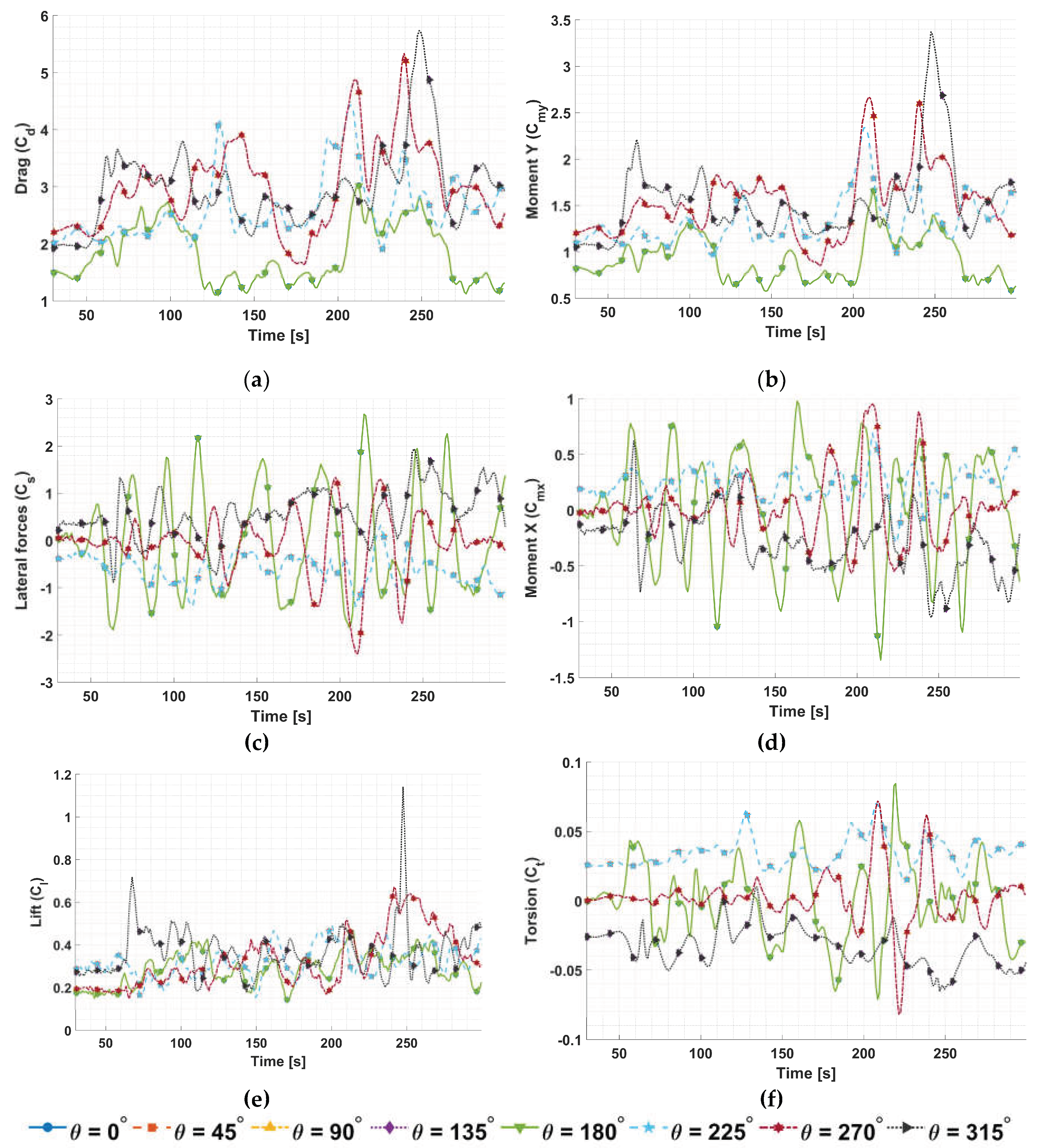
In contrast, the SSTDDES formulation explicitly resolves large-scale vortices and sub-grid turbulent fluctuations in separated flow zones, allowing it to capture the extreme aerodynamic peaks. For example, Figure A3 and Figure A4 in Appendix A show that drag and moment Y have high peaks compared to the time history for all turbulence models around = 250 seconds.
In 50. 08% greater on average than the RANS prediction, and this amplification is observed across all parameters: on average, 202.15% higher for side forces, 51.87% higher for moment Y, 226.80% higher for moment X, and 204.73% higher for torsion compared to SST peak values. These divergences persist in the neighborhood configuration, where SSTDDES predicts a peak drag 48.68% higher and peak side forces 143.18% higher on average than SST. These results are consistent with previous studies showing that hybrid approaches improved predictive fidelity for boundary layer separation and vortex formation and, for structural design purposes, relying solely on RANS models, can underestimate important peak and fluctuating load effects, especially in separated-flow regions, reinforcing the necessity of models that can capture turbulent fluctuations to evaluate peak structural forces [25,61,62].
The introduction of a surrounding neighborhood alters the wind flow patterns, inducing aerodynamic interference effects on the structure. In terms of mean aerodynamic forces, the urban canopy generally acts as a shielding mechanism, creating a protective zone that mitigates the magnitude of most global coefficients: considering the average values of all evaluated wind incidence angles, mean drag is 17.91% higher in the isolated SST scenario and 20.43% higher in the isolated SSTDDES scenario when compared to their respective neighborhood configurations. Similarly, the mean lift force is 23.58% greater in the isolated RANS case and 20.26% greater in the SSTDDES case, demonstrating that upstream structures reduce the direct aerodynamic loads acting on the facades of the target building.
However, despite this overall reduction in the mean coefficients, the neighborhood configuration introduces some interference phenomena that amplify transient peak forces. While the mean lift experiences a reduction, the peak lift values are amplified by the surrounding urban geometry, measuring 16.47% higher in the RANS configuration compared to the isolated case. Torsional behavior further exemplifies this wake-induced phenomenon, since in the RANS isolated models, maximum torsion values remain close to zero. Yet, the presence of the neighborhood introduces asymmetric flow separation and turbulent wakes that amplify torsional effects across all angles, resulting in peak torsion values that are 21.52% higher than those in the isolated setup, indicating that the adjacent buildings induce twisting loads that do not exist when the building stands alone. This type of behavior, which is specific to each region, topography, and morphology of the building distribution within a city, cannot be determined in a generalized manner through normative approaches, demonstrating that numerical and experimental tests with specific setups may be necessary for urban planning and the design of new buildings.
In the isolated configuration, the peak torsional coefficient shows different angle-dependent trends in the RANS and SSTDDES results. This divergence is consistent with modeling strategies: steady RANS responds primarily to the mean asymmetric pressure field induced by oblique wind incidence, whereas SSTDDES with turbulent inflow also captures instantaneous vortex shedding and fluctuating pressure asymmetry. For this reason, torsional peaks in SSTDDES do not need to follow the same monotonic variation with wind angle seen in RANS, as the literature supports linking this behavior to both turbulence-model formulation and incoming turbulence, since changes in angle of direct incidence and inflow turbulence can modify separation, shedding mode, and fluctuating torsional loading [60,63,64].
The most notable deviation from the general shielding effect is observed in the lateral dynamics which, contrary to drag and vertical forces, both mean and maximum side forces are amplified by the neighborhood across the majority of evaluated angles, peaking in the SSTDDES neighborhood configuration at an incidence angle of = 180°, where the wind strikes directly the smaller facade, reaching a maximum coefficient of = 2.59. At this specific angle, upstream wake interactions and localized negative pressure fields generated by adjacent structures likely exacerbate lateral shedding and crosswind instability.
Ultimately, these results indicate that while urban densification may provide a general shielding effect against mean longitudinal wind loads, it concurrently generates highly turbulent, localized wakes that amplify transient peak forces in both evaluated turbulence models, with side forces and torsional moments showing the largest differences between isolated and neighborhood configurations. These amplifications underscore the necessity of modeling specific urban surroundings to ensure structural safety and adequately capture wind effects for the potential structural design of the building.
Furthermore, to assess a deeper understanding of the numerical simulations, the aerodynamic coefficients obtained for the isolated configuration were compared with data from literature. However, a particularity adopted in the present study regarding reference quantities should be highlighted, as the reference area used to calculate the drag coefficient was kept constant and equal to the smaller face of the building (proportions 1:6). Since literature frequently uses the larger projected face of the model as the reference area (proportions 1.5:6), the values extracted from previous studies were multiplied by an adjustment factor of 1.5 to allow for an equitable comparison with the results of the present numerical modeling.
When evaluating the scenarios with wind perpendicular to the building faces, a good agreement between the numerical and experimental results was observed, since for = 0°, the numerical models yielded a mean = 1.33 for the SST and = 1.22 for the SSTDDES, with wind tunnel experiments reported in Alminhana et al. [65] reporting approximately = 0.80 based on the larger face. After applying the area conversion factor, the adjusted value is 1.20, indicating that the RANS and SSTDDES formulations yielded a relative difference of approximately 9.77% and 1.64%, respectively, compared with the experimental data, demonstrating good predictive agreement in capturing the mean flow topology.
For = 90°, the simulations yielded = 2.14 for RANS and = 2.01 for SSTDDES. The literature indicates that experimental values are sensitive to the intensity of the incoming turbulence, with Elshaer et al. [38] reporting that the transition from uniform flow to a boundary-layer profile increased from 1.49 to 1.80. Yan and Li [66], using the same larger face as the reference area, reported values of 1.50 for smooth flow and 1.80 for turbulent flow, while Alminhana et al. [65] obtained values of 1.45 and 1.24 for smooth and turbulent flow, respectively. By converting the most conservative range in the literature (1.24 < < 1.50) to the reference area adopted in this study, the expected values range from 1.86 to 2.25, with both models agreeing well with the turbulent-flow conditions.
At = 45°, the values were = 1.95 for RANS and = 1.75 for SSTDDES, while experimental data from Alminhana et al. [65] showed a value of = 1.65 after adjusting for the reference area. Thus, the RANS and SSTDDES formulations exhibited, respectively, a deviation of approximately 15.38% and 5.71%, demonstrating that both models can capture the effects observed in experimental tests, although the DDES model is more consistent with what is expected in this case.
Recent studies suggest parameterizing the drag coefficient as a function of building geometry to improve urban canopy models and predictions. Chen et al. [67] demonstrated that cross-sectional geometry alters recirculation zones, indicating that macroscopic estimates based solely on frontal area density or plan area density may exhibit discrepancies. When evaluating the parametric formulation proposed by Santiago and Martilli [68], which relates drag to plan area density for sparse flows, the values for isolated rectangular geometries typically range from 1.08 to 1.35, with a limiting upper value of 1.85 for dense arrays. The results obtained in the present study are in good agreement with this range of parametric estimates, since for a = 0° incidence angle, corresponding flow impinging on the smaller facade, the models yielded = 1.22 for SSTDDES and = 1.33 for RANS. At = 90°, after correcting the coefficient based on the frontal area effectively projected to the wind, the actual aerodynamic shape coefficients are 1.34 for SSTDDES and 1.42 for RANS, confirming the consistency of the simulations with the parameterization ranges for tall buildings. Furthermore, inspired by the pronounced variations in drag observed for different morphologies, the presented results allow a directional parameterization to be proposed for the CAARC configuration: variations in the wind incidence angle modify the apparent “aerodynamic shape” and recirculation wake, yielding a drag distribution curve that can be directly incorporated into future mesoscale predictive models to represent buildings with a 1:1.5 aspect ratio more accurately than the use of a single static coefficient.
6. Conclusions
This study presented a numerical investigation of the aerodynamic loads on a CAARC high-rise building placed within a dense urban neighborhood in Oklahoma City and, by using CFD simulations, the influence of the surrounding urban geometry and multiple wind incidence angles were examined. The analysis evaluated aerodynamic coefficients, while comparing the RANS SST and the SSTDDES turbulence models.
The results demonstrated a sensitivity of aerodynamic loads to urban geometry and wind direction. Analysis revealed that wind incidence angles of 90° and 270° generated the highest mean drag and overturning moments, as the airflow directly impacts the larger facade of the building. Conversely, oblique incidence angles amplified torsional effects and, while the surrounding neighborhood generally provided a shielding effect that reduced mean structural loads, it concurrently induced complex wake interactions that amplified localized transient peak forces, particularly lateral side forces and peak torsion.
Furthermore, the comparison between the turbulence models revealed that steady-state formulations might misrepresent the nature of certain peak loads. While RANS predicted torsional peaks driven by mean geometric asymmetries at oblique angles, the SSTDDES captured instantaneous alternating vortex shedding at normal incidence angles ( = 0° and 90°), suggesting that resolving transient fluctuations is important, as mean-flow symmetries might fail to represent the shedding mechanics that drive extreme bluff body twisting. Additionally, the evaluation of the drag coefficients corroborated literature parameterization theories, and for future work, the proposal of directional coefficient distribution curves could offer a more precise and consistent input for future mesoscale predictive models representing buildings with the same base proportions as the CAARC building and other geometries.
Overall, the findings suggest that aerodynamic interactions in high-density urban environments are complex and oversimplified analytical methods or steady-state assumptions may result in the underestimation of extreme peak loads. The spatial arrangement of the buildings, combined with their orientation relative to prevailing winds, must be considered during early-stage urban design and new buildings development. This study underscores the value of CFD-based wind engineering analysis to ensure structural safety.
Limitations of the Research and Recommendations for Future Work
Despite the findings provided by this investigation, certain limitations should be acknowledged and addressed in future research. Regarding turbulence modeling, this study focused on the comparison between RANS and SSTDDES formulations; however, a full Large-Eddy Simulation (LES) model was not explored. While RANS is adequate for predicting mean velocity fields, it is inherently deficient in capturing turbulence intensity and gustiness. Future studies should conduct a comprehensive comparative analysis involving RANS, DDES and LES frameworks, confronting the computational processing time of each approach with its accuracy and computational viability for structural projects. Also, the current research concentrated on a scenario where the central high-rise prominently stands out above the surrounding urban canopy. Future investigations should examine cases where the target building possesses a height equal or lower than its neighboring structures.
The current study investigates the CAARC model, which features a standard rectangular cross-section with sharp corners, while modern architectural designs could employ aerodynamic shaping, such as chamfered, recessed or round corners to mitigate wind loads. Future research could evaluate how these geometric modifications perform when subjected to complex, highly turbulent wakes of a dense neighborhood, it may alter the aerodynamic effectiveness of such mitigation strategies.
While this research assumed a neutral ABL with isothermal conditions, densely built urban areas are subjected to Urban Heat Island effects, which introduces thermal stratification. Future CFD simulations should incorporate thermal buoyancy effects to evaluate how temperature-driven turbulence modulates boundary layer separation, wake recovery and the resulting aerodynamic forces on high-rise buildings.
Finally, the building model was considered perfectly rigid and, given the transient peak forces captured by the SSTDDES model, particularly the crosswind and torsional loads, future investigations should couple the CFD routine with a Computation Structural Dynamics module. Evaluating fluid-structure interaction could allow the assessment of aeroelastic phenomena, such as vortex-induced vibrations and aerodynamic damping, which are important for fatigue and serviceability analysis of slender buildings.
Author Contributions
P.U.d.S.: conceptualization, software, validation, formal analysis, investigation, resources, data curation, writing—original draft preparation, and visualization. G.B.: conceptualization, methodology, investigation, writing—review and editing, supervision, and project administration. M.G.: resources, writing—review and editing, supervision, and project administration. All authors have read and agreed to the published version of the manuscript.
Funding
Fundação de Coordenação de Aperfeiçoamento de Pessoal de Nível Superior (CAPES)—Finance Code 001 and Conselho Nacional de Desenvolvimento Científico e Tecnológico (CNPq)—302119/2022-1.
Data Availability Statement
The original data presented in the study are openly available in https://github.com/p-ulisses/openfoam-phd-ufmg-propees/ as a minimum dataset to run the files in OpenFOAM v2206.
Acknowledgments
The authors would like to thank Fundação de Coordenação de Aperfeiçoamento de Pessoal de Nível Superior (CAPES) and the Conselho Nacional de Desenvolvimento Científico e Tecnológico (CNPq) for funding this work. The authors would also like to thank Centro Nacional de Processamento de Alto Desempenho em São Paulo (CENAPAD-SP) at Universidade Estadual de Campinas (UNICAMP) for providing High-Performance Computing resources for this research.
Conflicts of Interest
The authors declare no conflicts of interest.
Abbreviations
The following abbreviations are used in this manuscript:
| ABL | Atmospheric Boundary Layer |
| ABNT | Associação Brasileira de Normas Técnicas |
| CAARC | Commonwealth Advisory Aeronautical Research Council |
| COST | European Cooperation in Science and Technology |
| CFD | Computational Fluid Dynamics |
| DES | Detached-Eddy Simulations |
| GAMG | Geometric-Algebraic Multi-Grid |
| HPC | High-Performance Computing |
| LES | Large-Eddy Simulations |
| RANS | Reynolds-Averaged Navier-Stokes |
| SST | Shear Stress Transport |
| SSTDDES | Shear Stress Transport Delayed Detached-Eddy Simulations |
| TKE | Turbulent Kinetic Energy |
| UCL | Urban Canopy Layer |
Appendix A
Appendix A.1
This appendix contains the numerical values of the aerodynamic coefficients presented in Section 5 of this study. It also provides the numerical convergence histories for the RANS model (where the “Time [s]” axis represents pseudo-time iterations) and the actual time-domain plots for the SSTDDES model. Table A1, Table A2, Table A3 and Table A4 present the aerodynamic coefficient data, while Figure A1, Figure A2, Figure A3 and Figure A4 show the corresponding convergence and time-domain plots.

Table A1.
Numerical values of the aerodynamic coefficients considering the RANS SST model in the isolated configuration.
Table A1.
Numerical values of the aerodynamic coefficients considering the RANS SST model in the isolated configuration.
| Coefficient | Data values | 0° | 45° | 90° | 135° | 180° | 225° | 270° | 315° |
|---|---|---|---|---|---|---|---|---|---|
| Drag | Mean | 1.33 | 1.95 | 2.14 | 1.95 | 1.33 | 1.95 | 2.14 | 1.95 |
| Peak | 1.57 | 2.01 | 2.64 | 2.01 | 1.57 | 2.01 | 2.64 | 2.01 | |
| Lateral forces | Mean | -0.01 | -0.39 | 0.00 | 0.39 | -0.01 | -0.39 | 0.00 | 0.39 |
| Peak | 0.26 | 0.74 | 0.20 | 0.66 | 0.26 | 0.74 | 0.20 | 0.66 | |
| Lift | Mean | 0.85 | 1.08 | 0.86 | 1.08 | 0.85 | 1.08 | 0.86 | 1.08 |
| Peak | 1.18 | 1.65 | 1.94 | 1.45 | 1.18 | 1.65 | 1.94 | 1.45 | |
| Overturning Moment Y | Mean | 0.73 | 1.06 | 1.17 | 1.06 | 0.73 | 1.06 | 1.17 | 1.06 |
| Peak | 0.87 | 1.08 | 1.38 | 1.08 | 0.87 | 1.08 | 1.38 | 1.08 | |
| Overturning Moment X | Mean | 0.00 | 0.21 | 0.00 | -0.21 | 0.00 | 0.21 | 0.00 | -0.21 |
| Peak | 0.12 | 0.32 | 0.07 | 0.29 | 0.12 | 0.32 | 0.07 | 0.29 | |
| Torsion | Mean | 0.00 | 0.43 | 0.00 | -0.43 | 0.00 | 0.43 | 0.00 | -0.43 |
| Peak | 0.10 | 0.45 | 0.06 | 0.45 | 0.10 | 0.45 | 0.06 | 0.45 |
Table A2.
Numerical values of the aerodynamic coefficients considering the SSTDDES model in the isolated configuration.
Table A2.
Numerical values of the aerodynamic coefficients considering the SSTDDES model in the isolated configuration.
| Coefficient | Data | 0° | 45° | 90° | 135° | 180° | 225° | 270° | 315° |
|---|---|---|---|---|---|---|---|---|---|
| Drag | Mean | 1.22 | 1.75 | 2.01 | 2.00 | 1.22 | 1.75 | 2.01 | 2.00 |
| Peak | 2.04 | 2.95 | 3.56 | 3.82 | 2.04 | 2.95 | 3.56 | 3.82 | |
| Lateral forces | Mean | -0.03 | -0.42 | -0.05 | 0.39 | -0.03 | -0.42 | -0.05 | 0.39 |
| Peak | 1.78 | 0.93 | 1.60 | 1.30 | 1.78 | 0.93 | 1.60 | 1.30 | |
| Lift | Mean | 0.77 | 0.85 | 0.87 | 0.99 | 0.77 | 0.85 | 0.87 | 0.99 |
| Peak | 1.24 | 1.30 | 1.79 | 3.04 | 1.24 | 1.30 | 1.79 | 3.04 | |
| Overturning Moment Y | Mean | 0.61 | 0.89 | 1.02 | 1.03 | 0.61 | 0.89 | 1.02 | 1.03 |
| Peak | 1.11 | 1.56 | 1.78 | 2.25 | 1.11 | 1.56 | 1.78 | 2.25 | |
| Overturning Moment X | Mean | 0.01 | 0.16 | 0.02 | -0.18 | 0.01 | 0.16 | 0.02 | -0.18 |
| Peak | 0.90 | 0.46 | 0.64 | 0.64 | 0.90 | 0.46 | 0.64 | 0.64 | |
| Torsion | Mean | 0.00 | 0.37 | 0.03 | -0.35 | 0.00 | 0.37 | 0.03 | -0.35 |
| Peak | 0.90 | 0.75 | 0.87 | 0.70 | 0.90 | 0.75 | 0.87 | 0.70 |
Table A3.
Numerical values of the aerodynamic coefficients considering the RANS SST model in the neighborhood configuration.
Table A3.
Numerical values of the aerodynamic coefficients considering the RANS SST model in the neighborhood configuration.
| Coefficient | Data | 0° | 45° | 90° | 135° | 180° | 225° | 270° | 315° |
|---|---|---|---|---|---|---|---|---|---|
| Drag | Mean | 1.11 | 1.35 | 1.77 | 1.93 | 1.29 | 1.42 | 1.87 | 1.37 |
| Peak | 1.14 | 1.39 | 1.88 | 1.98 | 1.37 | 1.47 | 1.91 | 1.42 | |
| Lateral forces | Mean | 0.11 | -0.13 | -0.02 | 0.37 | 0.19 | -0.08 | 0.05 | 0.44 |
| Peak | 0.61 | 0.21 | 0.24 | 0.48 | 0.35 | 0.24 | 0.86 | 0.55 | |
| Lift | Mean | 0.81 | 0.68 | 0.69 | 0.76 | 0.77 | 0.85 | 0.60 | 0.75 |
| Peak | 1.78 | 1.93 | 1.77 | 1.78 | 1.75 | 2.10 | 1.73 | 1.64 | |
| Overturning Moment Y | Mean | 0.67 | 0.80 | 1.05 | 0.97 | 0.70 | 0.86 | 1.05 | 0.83 |
| Peak | 0.71 | 0.81 | 1.11 | 0.99 | 0.76 | 0.88 | 1.11 | 0.86 | |
| Overturning Moment X | Mean | -0.05 | 0.10 | 0.00 | -0.19 | -0.31 | 0.08 | -0.04 | -0.25 |
| Peak | 0.40 | 0.15 | 0.14 | 0.27 | 0.14 | 0.16 | 0.57 | 0.31 | |
| Torsion | Mean | -0.02 | 0.28 | -0.13 | -0.47 | 0.07 | 0.26 | -0.04 | -0.30 |
| Peak | 0.46 | 0.36 | 0.23 | 0.52 | 0.15 | 0.30 | 0.18 | 0.38 |
Table A4.
Numerical values of the aerodynamic coefficients considering the SSTDDES model in the neighborhood configuration.
Table A4.
Numerical values of the aerodynamic coefficients considering the SSTDDES model in the neighborhood configuration.
| Coefficient | Data | 0° | 45° | 90° | 135° | 180° | 225° | 270° | 315° |
|---|---|---|---|---|---|---|---|---|---|
| Drag | Mean | 1.12 | 1.24 | 1.47 | 1.87 | 1.42 | 1.11 | 1.71 | 1.17 |
| Peak | 1.81 | 1.62 | 2.59 | 3.03 | 3.78 | 1.74 | 2.58 | 1.51 | |
| Lateral forces | Mean | 0.09 | -0.05 | -0.02 | 0.42 | 0.30 | -0.02 | 0.06 | 0.32 |
| Peak | 1.31 | 0.93 | 0.52 | 1.20 | 2.59 | 0.61 | 0.68 | 0.76 | |
| Lift | Mean | 0.85 | 0.66 | 0.59 | 0.74 | 0.86 | 0.65 | 0.55 | 0.65 |
| Peak | 1.60 | 1.31 | 1.22 | 2.42 | 2.01 | 1.20 | 1.90 | 2.49 | |
| Overturning Moment Y | Mean | 0.65 | 0.71 | 0.85 | 0.90 | 0.72 | 0.65 | 0.94 | 0.72 |
| Peak | 1.02 | 1.00 | 1.53 | 1.42 | 1.93 | 1.03 | 1.43 | 0.93 | |
| Overturning Moment X | Mean | -0.05 | 0.06 | 0.02 | -0.23 | -0.10 | 0.01 | -0.05 | -0.18 |
| Peak | 0.83 | 0.47 | 0.40 | 0.65 | 1.07 | 0.33 | 0.51 | 0.46 | |
| Torsion | Mean | -0.06 | 0.16 | -0.06 | -0.42 | 0.08 | 0.13 | -0.07 | -0.24 |
| Peak | 0.74 | 0.50 | 0.67 | 0.77 | 0.77 | 0.36 | 0.47 | 0.42 |
Figure A1.
Convergence histories of the aerodynamic coefficients of the neighborhood configuration using the RANS SST turbulence model: (a) drag, (b) moment Y, (c) lateral forces, (d) moment X, (e) lift and (f) torsion.
Figure A1.
Convergence histories of the aerodynamic coefficients of the neighborhood configuration using the RANS SST turbulence model: (a) drag, (b) moment Y, (c) lateral forces, (d) moment X, (e) lift and (f) torsion.
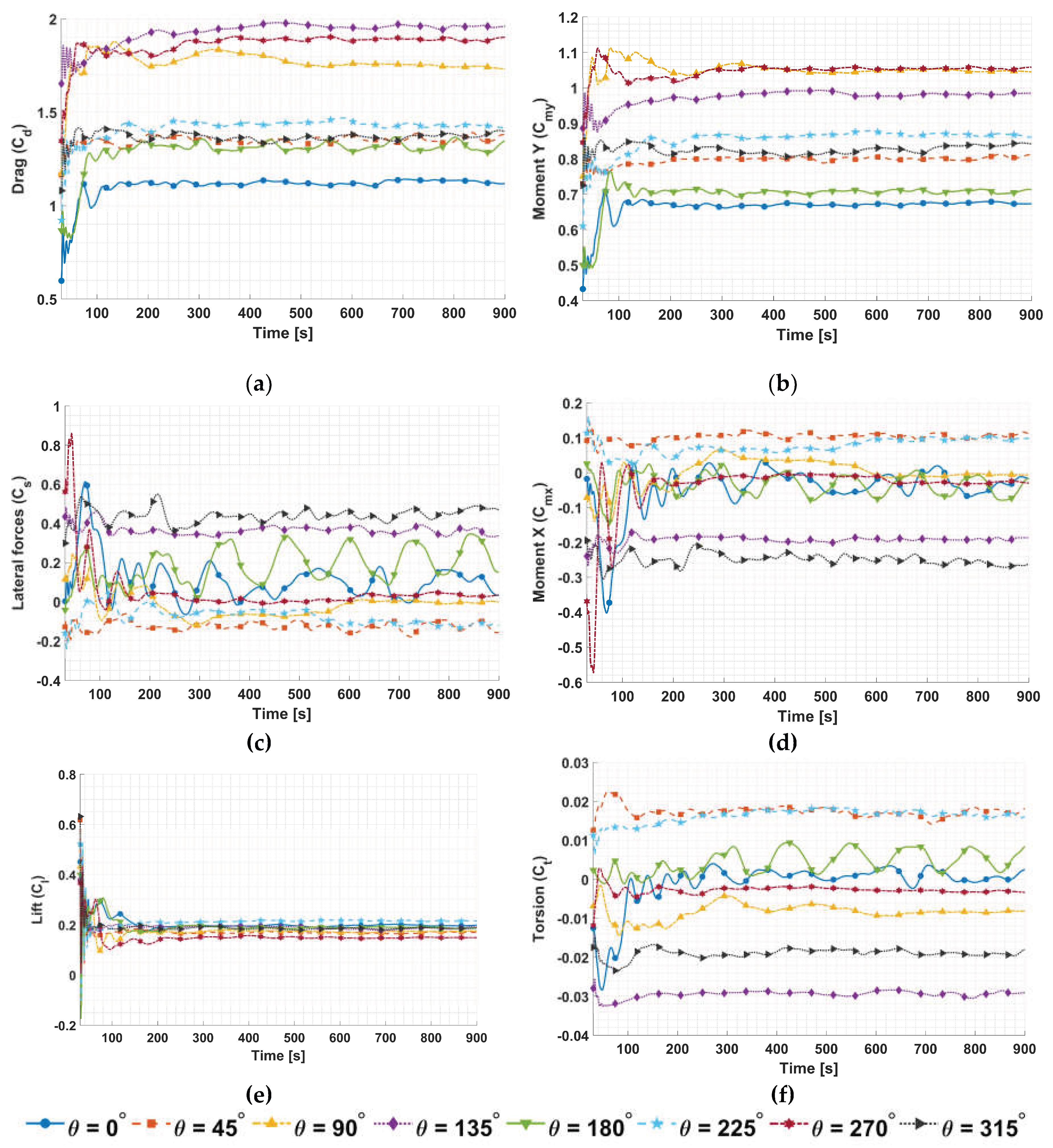
Figure A2.
Convergence histories of the aerodynamic coefficients of the isolated configuration using the RANS SST turbulence model: (a) drag, (b) moment Y, (c) lateral forces, (d) moment X, (e) lift and (f) torsion.
Figure A2.
Convergence histories of the aerodynamic coefficients of the isolated configuration using the RANS SST turbulence model: (a) drag, (b) moment Y, (c) lateral forces, (d) moment X, (e) lift and (f) torsion.
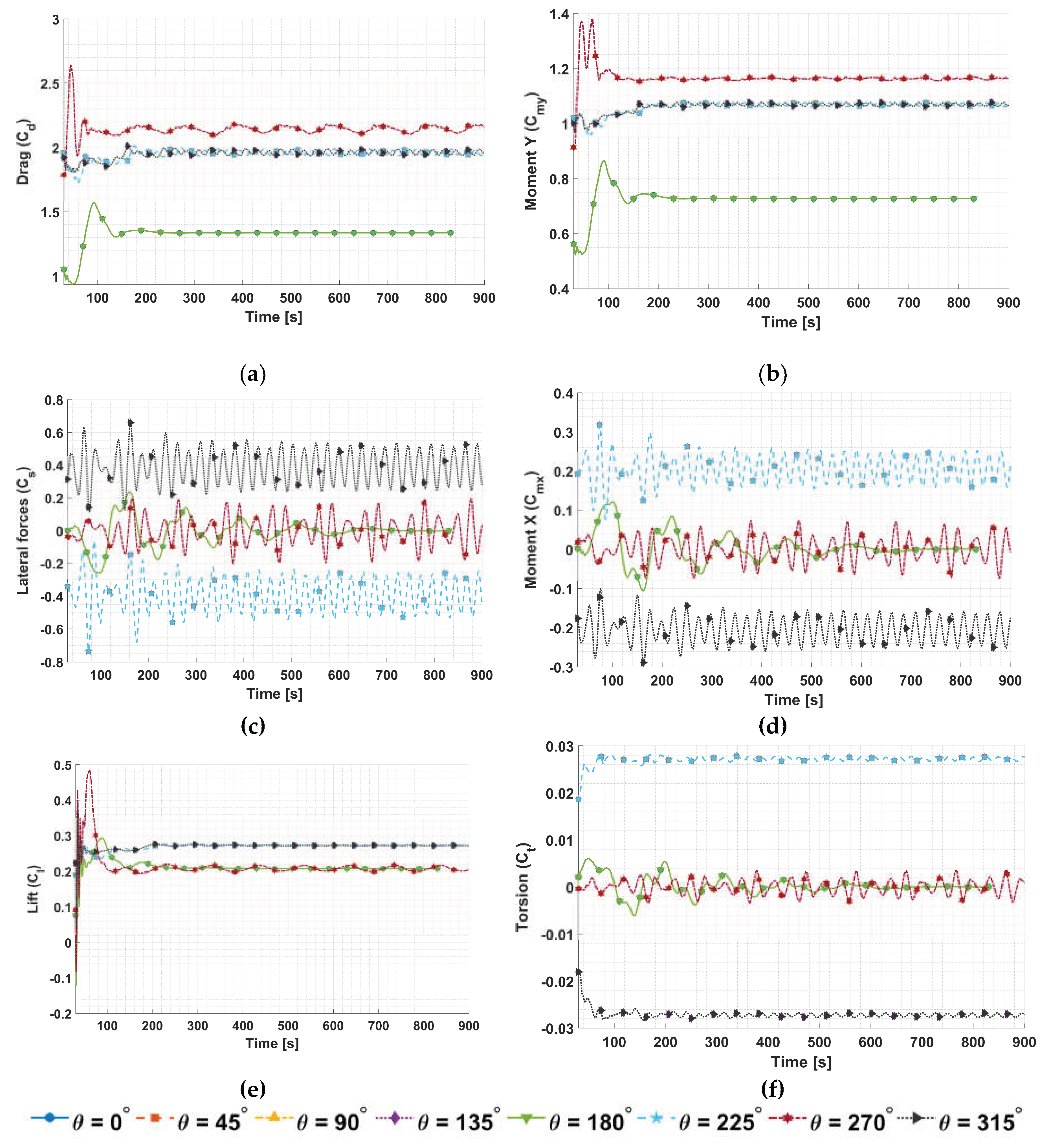
Figure A3.
Time-domain plot of the aerodynamic coefficients of the neighborhood configuration using the SSTDDES turbulence model: (a) drag, (b) moment Y, (c) lateral forces, (d) moment X, € lift and (f) torsion.
Figure A3.
Time-domain plot of the aerodynamic coefficients of the neighborhood configuration using the SSTDDES turbulence model: (a) drag, (b) moment Y, (c) lateral forces, (d) moment X, € lift and (f) torsion.
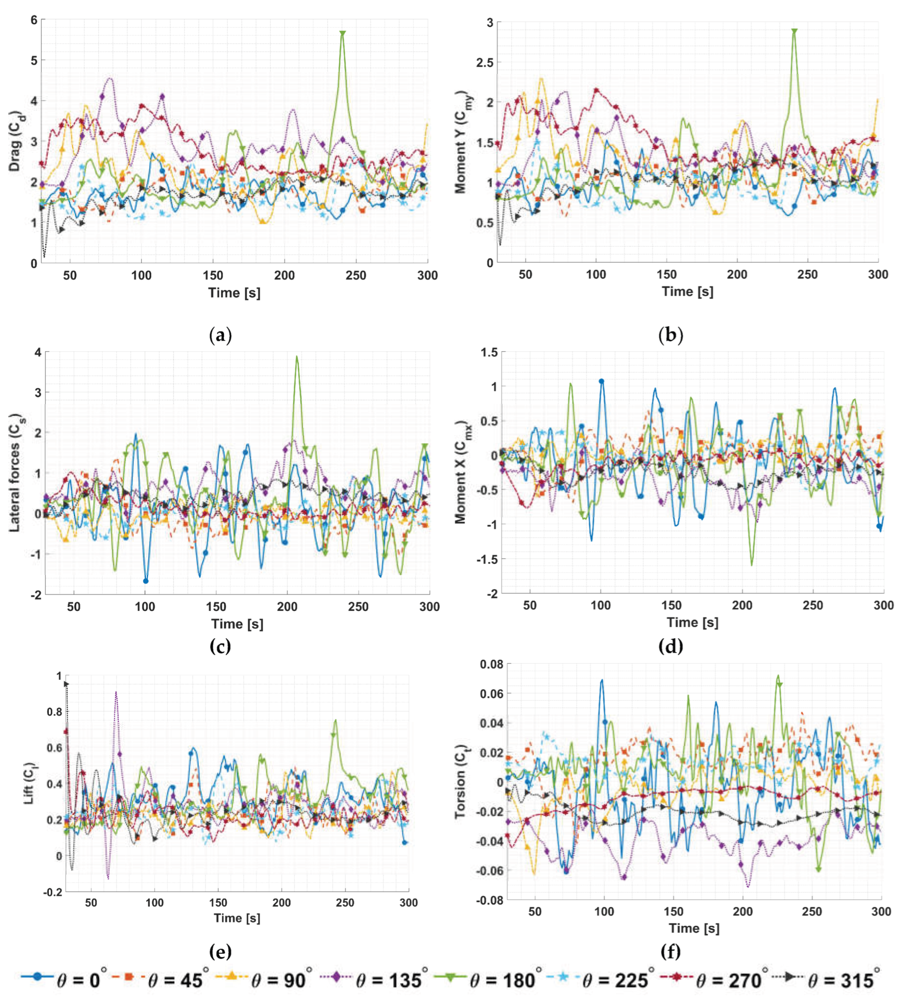
Figure A4.
Time-domain plot of the aerodynamic coefficients of the isolated configuration using the SSTDDES turbulence model: (a) drag, (b) moment Y, (c) lateral forces, (d) moment X, (e) lift and (f) torsion.
Figure A4.
Time-domain plot of the aerodynamic coefficients of the isolated configuration using the SSTDDES turbulence model: (a) drag, (b) moment Y, (c) lateral forces, (d) moment X, (e) lift and (f) torsion.
References
- Caswell, H.; Alidoust, S.; Corcoran, J. Planning for livable compact vertical cities: A quantitative systematic review of the impact of urban geometry on thermal and visual comfort in high-rise precincts. Sustain. Cities Soc. 2025, 119, 106007. [Google Scholar] [CrossRef]
- Ding, C. Building height restrictions, land development and economic costs. Land Use Policy 2013, 30, 485–495. [Google Scholar] [CrossRef]
- Siddique, M.A.; Boqing, F.; Dongyun, L. Modeling the Impact and Risk Assessment of Urbanization on Urban Heat Island and Thermal Comfort Level of Beijing City, China (2005–2020). Sustainability 2023, 15, 6043. [Google Scholar] [CrossRef]
- Chen, L.; Hang, J.; Sandberg, M.; Claverie, R.; Buccolieri, R.; Di Sabatino, S. The impacts of building height variations and building packing densities on flow adjustment and city breathability in idealized urban models. Build. Environ. 2017, 118, 344–361. [Google Scholar] [CrossRef]
- Simões, T.; Estanqueiro, A. A new methodology for urban wind resource assessment. Renew. Energy 2016, 89, 598–605. [Google Scholar] [CrossRef]
- Abohela, I.; Sundararajan, R. Analytical Review of Wind Assessment Tools for Urban Wind Turbine Applications. Atmosphere 2024, 15, 1049. [Google Scholar] [CrossRef]
- Tominaga, Y.; Shirzadi, M.; Mochida, A.; Blocken, B. Accuracy of CFD simulations in urban aerodynamics and microclimate: Progress and challenges. Build. Environ. 2023, 243, 110723. [Google Scholar] [CrossRef]
- Wijesooriya, K.; Mohotti, D.; Amin, A.; Chauhan, K. A technical review of computational fluid dynamics (CFD) applications on wind design of tall buildings and structures: Past, present and future. J. Build. Eng. 2023, 74, 106828. [Google Scholar] [CrossRef]
- Hui, Y.; Tang, Y.; Yang, Q.; Mochida, A. Numerical study on influence of surface vegetation on aerodynamics of high-rise buildings. Sustain. Cities Soc. 2024, 107, 105407. [Google Scholar] [CrossRef]
- Silva, P.U.d.; Bono, G.; Greco, M. Assessing Pedestrian Comfort in Dense Urban Areas Using CFD Simulations: A Study on Wind Angle and Building Height Variations. Fluids 2025, 10, 233. [Google Scholar] [CrossRef]
- Villalobos-García, C.; Pérez-Moreno, L.F.; Arjona-Catzim, I.F.; Rico-García, E. Wind Effects of Surrounding Structures in an Urban Area on a High-Rise Building by Computational Fluid Dynamics. Wind 2026, 6, 16. [Google Scholar] [CrossRef]
- Ibarra-Hernández, C.; Hernández-García, L.; Nájera-Sanchez, R.; Arriaga-Gomez, E.; Martínez-Delgadillo, S.; Medellín-Salazar, D.; García, A.A. Turbulent Flow Analysis of a Representative Low-Height Urban Landscape in Mexico. Fluids 2026, 11, 23. [Google Scholar] [CrossRef]
- Xi, C.; Ren, C.; Wang, J.; Feng, Z.; Cao, S.-J. Impacts of urban-scale building height diversity on urban climates: A case study of Nanjing, China. Energy Build. 2021, 251, 111350. [Google Scholar] [CrossRef]
- Guo, X.; Wang, L. Implementation and assessment of a hybrid RANS/LES model using OpenFOAM. J. Wind Eng. Ind. Aerodyn. 2025, 263, 106113. [Google Scholar] [CrossRef]
- Associação Brasileira de Normas Técnicas. ABNT NBR 6123: Forças devidas ao vento em edificações; ABNT. Rio de Janeiro, Brazil, 2023.
- Liu, M.; Wang, X. Three-Dimensional Wind Field Construction and Wind Turbine Siting in an Urban Environment. Fluids 2020, 5, 137. [Google Scholar] [CrossRef]
- Guillas, S.; Glover, N.; Malki-Epshtein, L. Bayesian calibration of the constants of the k–ε turbulence model for a CFD model of street canyon flow. Comput. Methods Appl. Mech. Eng. 2014, 279, 536–553. [Google Scholar] [CrossRef]
- Shirzadi, M.; Mirzaei, P.A.; Naghashzadegan, M. Improvement of k-epsilon turbulence model for CFD simulation of atmospheric boundary layer around a high-rise building using stochastic optimization and Monte Carlo Sampling technique. J. Wind Eng. Ind. Aerodyn. 2017, 171, 366–379. [Google Scholar] [CrossRef]
- Houda, S.; Belarbi, R.; Zemmouri, N. A CFD Comsol model for simulating complex urban flow. Energy Procedia 2017, 139, 373–378. [Google Scholar] [CrossRef]
- Corson, D.; Jaiman, R.; Shakib, F. Industrial application of RANS modelling: capabilities and needs. Int. J. Comput. Fluid Dyn. 2009, 23, 337–347. [Google Scholar] [CrossRef]
- International Organization for Standardization. ISO 2533:1975; Standard Atmosphere. ISO: Geneva, Switzerland, 1975.
- Menter, F.R. Two-equation eddy-viscosity turbulence models for engineering applications. AIAA J. 1994, 32, 1598–1605. [Google Scholar] [CrossRef] [PubMed]
- turbulence model revisited. AIAA J. 2008, 46, 2823–2838. [CrossRef]
- Strelets, M. Detached eddy simulation of massively separated flows. In Proceedings of the 39th AIAA Aerospace Sciences Meeting and Exhibit, Reno, NV, USA, 8–11 January 2001. AIAA Paper 2001-0879. [Google Scholar] [CrossRef]
- Spalart, P.R.; Deck, S.; Shur, M.L.; Squires, K.D.; Strelets, M.K.; Travin, A. A new version of detached-eddy simulation, resistant to ambiguous grid densities. Theor. Comput. Fluid Dyn. 2006, 20, 181–195. [Google Scholar] [CrossRef]
- Shear Stress Transport Model. Flow Turbul. Combust. 2012, 88, 431–449. [CrossRef]
- Kolmogorov, A.N. The local structure of turbulence in incompressible viscous fluid for very large Reynolds numbers. Proc. R. Soc. Lond. Ser. A Math. Phys. Sci. 1991, 434, 9–13. [Google Scholar] [CrossRef]
- Smagorinsky, J. General circulation experiments with the primitive equations I. The basic experiment. Mon. Weather Rev. 1963, 91, 99–164. [Google Scholar]
- Dagnew, A.; Bitsuamlak, G.; Merrick, R. Computational evaluation of wind pressures on tall buildings. In Proceedings of the 11th Americas Conference on Wind Engineering, San Juan, Puerto Rico, 22–26 June 2009; Available online: https://www.researchgate.net/publication/271197966_Computational_evaluation_of_wind_pressures_on_tall_buildings.
- American Society of Civil Engineers. ASCE/SEI 7-22: Minimum Design Loads and Associated Criteria for Buildings and Other Structures; ASCE: Reston, VA, USA, 2022. [Google Scholar]
- European Committee for Standardization. EN 1991-1-1: Eurocode 1: Actions on structures - Part 1-1: General actions - Densities, self-weight, imposed loads for buildings; CEN. Brussels, Belgium, 2002.
- Ministry of Housing and Urban-Rural Constructions of the People's Republic of China. GB 50009-2012: Load Code for the Design of Building Structures; MOHURD. Beijing, China, 2012.
- Silva, P.U.d.; Bono, G.; Greco, M. Application of Topology Optimization as a Tool for the Design of Bracing Systems of High-Rise Buildings. Buildings 2025, 15, 1180. [Google Scholar] [CrossRef]
- Blessmann, J. Aerodinâmica das Construções I, 3rd ed.; Editora da UFRGS: Porto Alegre, Brazil, 2011. [Google Scholar]
- Mirzaei, P.A. CFD modeling of micro and urban climates: Problems to be solved in the new decade. Sustain. Cities Soc. 2021, 69, 102839. [Google Scholar] [CrossRef]
- Li, J.; Guo, F.; Chen, H. A study on urban block design strategies for improving pedestrian-level wind conditions: CFD-based optimization and generative adversarial networks. Energy Build. 2024, 304, 113863. [Google Scholar] [CrossRef]
- Aboshosha, H.; Elshaer, A.; Bitsuamlak, G.T.; El Damatty, A. Consistent inflow turbulence generator for LES evaluation of wind-induced responses for tall buildings. J. Wind Eng. Ind. Aerodyn. 2015, 142, 198–216. [Google Scholar] [CrossRef]
- Elshaer, A.; Aboshosha, H.; Bitsuamlak, G.; El Damatty, A.; Dagnew, A. LES evaluation of wind-induced responses for an isolated and a surrounded tall building. Eng. Struct. 2016, 115, 179–195. [Google Scholar] [CrossRef]
- Elshaer, A.; Bitsuamlak, G.; El Damatty, A. Variations in wind load on tall buildings due to urban development. Sustain. Cities Soc. 2017, 34, 264–277. [Google Scholar] [CrossRef]
- Liu, J.; Zhang, X.; Zhang, M.; Xu, F. LES evaluation of the aerodynamic characteristics of high-rise building with horizontal ribs under atmospheric boundary layer flow. J. Build. Eng. 2023, 71, 106487. [Google Scholar] [CrossRef]
- Franke, J.; Hirsch, C.; Jensen, A.G.; Hibi, K.; Schatzmann, M.; Westbury, P.S.; Wright, N.G.; Stathopoulos, T.; Best, A.I. Recommendations on the use of CFD in wind engineering. In Proceedings of the International Conference on Urban Wind Engineering and Building Aerodynamics (COST C14), Sint-Genesius-Rode, Belgium, 5–7 May 2004. [Google Scholar]
- Tominaga, Y.; Mochida, A.; Yoshie, R.; Kataoka, H.; Nozu, T.; Yoshikawa, M.; Shirasawa, T. AIJ guidelines for practical applications of CFD to pedestrian wind environment around buildings. J. Wind Eng. Ind. Aerodyn. 2008, 96, 1749–1761. [Google Scholar] [CrossRef]
- Schatzmann, M.; Olesen, H.; Franke, J. (Eds.) COST 732 Model Evaluation Case Studies: Approach and Results; Meteorological Institute, University of Hamburg: Hamburg, Germany, 2010; ISBN 3-00-018312-4. [Google Scholar]
- Melbourne, W.H. Comparison of measurements on the CAARC standard tall building model in simulated model wind flows. J. Wind Eng. Ind. Aerodyn. 1980, 6, 73–88. [Google Scholar] [CrossRef]
- model in commercial CFD software to model the neutral atmospheric boundary layer. J. Wind Eng. Ind. Aerodyn. 2007, 95, 355–369. [CrossRef]
- Yang, Y.; Gu, M.; Chen, S.; Jin, X. New inflow boundary conditions for modelling the neutral equilibrium atmospheric boundary layer in computational wind engineering. J. Wind Eng. Ind. Aerodyn. 2009, 97, 88–95. [Google Scholar] [CrossRef]
- Richards, P.J.; Norris, S.E. Appropriate boundary conditions for computational wind engineering models revisited. J. Wind Eng. Ind. Aerodyn. 2011, 99, 257–266. [Google Scholar] [CrossRef]
- Hugenholtz, C.H.; Brown, O.W.; Barchyn, T.E. Estimating aerodynamic roughness length (Z0) from terrestrial laser scanning point cloud data over un-vegetated surfaces. Aeolian Res. 2013, 10, 161–169. [CrossRef]
- Poletto, R.; Craft, T.; Revell, A. A New Divergence Free Synthetic Eddy Method for the Reproduction of Inlet Flow Conditions for LES. Flow Turbul. Combust. 2013, 91, 519–539. [Google Scholar] [CrossRef]
- Agrawal, S.; Sanyal, P.; Roy, A. Assessment of the aerodynamic performance of unconventional building shapes using 3D steady RANS with SST turbulence model. J. Wind Eng. Ind. Aerodyn. 2022, 225, 104988. [Google Scholar] [CrossRef]
- Gimenez, J.M.; Bre, F. An enhanced SST model to predict airflows around isolated and urban buildings. Build. Environ. 2023, 237, 110321. [Google Scholar] [CrossRef]
- Tang, B.; Deng, Y.; Zhang, Z.; Zhou, Y.; Huang, L.; Chen, X. High-resolution simulation of the near-field pollutant dispersion in a nuclear power plant community with high-performance computing. J. Nonlinear Math. Phys. 2024, 31, 6. [Google Scholar] [CrossRef]
- Launder, B.E.; Spalding, D.B. The numerical computation of turbulent flows. Comput. Methods Appl. Mech. Eng. 1974, 3, 269–289. [Google Scholar] [CrossRef]
- Gariazzo, C.; Leitl, B.; Trini Castelli, S.; Baumann-Stanzer, K.; Reisin, T.G.; Barmpas, F.; Tinarelli, G.; Milliez, C.M.; Armand, P.; Bemporad, E. COST Action ES1006. Evaluation, improvement and guidance of local-scale emergency prediction and response tools for airborne hazards in built environments: Ongoing activities, experiments and recent results. Chem. Eng. Trans. 2014, 36, 529–534. [Google Scholar] [CrossRef]
- Rakai, A.; Kristóf, G. Microscale obstacle resolving air quality model evaluation with the Michelstadt case. Sci. World J. 2013, 2013, 781748. [Google Scholar] [CrossRef] [PubMed]
- Efthimiou, G.C.; Andronopoulos, S.; Bartzis, J.G. Prediction of dosage-based parameters from the puff dispersion of airborne materials in urban environments using the CFD-RANS methodology. Meteorol. Atmos. Phys. 2018, 130, 107–124. [Google Scholar] [CrossRef]
- Shaukat, U.; Hertwig, D.; Patruno, C.; Ricci, A.; Blocken, B. Validation of large eddy simulations in urban wind studies using a new overall area metric. Build. Environ. 2025, 267, 112285. [Google Scholar] [CrossRef]
- Shur, M.L.; Spalart, P.R.; Strelets, M.K.; Travin, A.K. A hybrid RANS-LES approach with delayed-DES and wall-modelled LES capabilities. Int. J. Heat Fluid Flow 2008, 29, 1638–1649. [Google Scholar] [CrossRef]
- Chaouat, B. The state of the art of hybrid RANS/LES modeling for the simulation of turbulent flows. Flow Turbul. Combust. 2017, 99, 279–327. [Google Scholar] [CrossRef] [PubMed]
- Guzmán-Solís, V.; Pozos-Estrada, A.; Gomez, R. Experimental study of wind-induced shear, bending, and torsional loads on rectangular tall buildings. Adv. Struct. Eng. 2020, 23, 2982–2995. [Google Scholar] [CrossRef]
- Dagnew, A.; Bitsuamlak, G.T. Computational evaluation of wind loads on buildings: A review. Wind Struct. 2013, 16, 629–660. [Google Scholar] [CrossRef]
- Heinz, S. A review of hybrid RANS-LES methods for turbulent flows: Concepts and applications. Prog. Aerosp. Sci. 2020, 114, 100597. [Google Scholar] [CrossRef]
- Yadav, H.; Roy, A.K. Wind-induced aerodynamic responses of triangular high-rise buildings with varying cross-section areas. Buildings 2024, 14, 2722. [Google Scholar] [CrossRef]
- Zhou, L.; Tse, K.T.; Hu, G. Experimental investigation on the aerodynamic characteristics of a tall building subjected to twisted wind. J. Wind Eng. Ind. Aerodyn. 2022, 224, 104976. [Google Scholar] [CrossRef]
- Alminhana, G.W.; Braun, A.L.; Loredo-Souza, A.M. A numerical-experimental investigation on the aerodynamic performance of CAARC building models with geometric modifications. J. Wind Eng. Ind. Aerodyn. 2018, 180, 34–48. [Google Scholar] [CrossRef]
- Yan, B.W.; Li, Q.S. Inflow turbulence generation methods with large eddy simulation for wind effects on tall buildings. Comput. Fluids 2015, 116, 158–175. [Google Scholar] [CrossRef]
- Chen, K.; Mo, Z.; Hang, J. The recirculation flow after different cross-section shaped high-rise buildings with applications to ventilation assessment and drag parameterization. Build. Simul. 2024, 17, 509–524. [Google Scholar] [CrossRef]
- Santiago, J.L.; Martilli, A. A dynamic urban canopy parameterization for mesoscale models based on computational fluid dynamics Reynolds-averaged Navier–Stokes microscale simulations. Bound.-Layer. Meteorol. 2010, 137, 417–439. [Google Scholar] [CrossRef]
Figure 1.
Atmospheric Boundary Layer and Urban Canopy Layer.
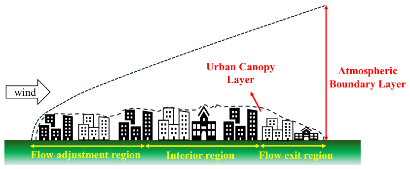
Figure 2.
Forces and moments acting on a building: (a) drag, side and lift forces with geometric parameters, (b) overturning moment Y, (c) overturning moment X and (d) torsional moment.
Figure 2.
Forces and moments acting on a building: (a) drag, side and lift forces with geometric parameters, (b) overturning moment Y, (c) overturning moment X and (d) torsional moment.
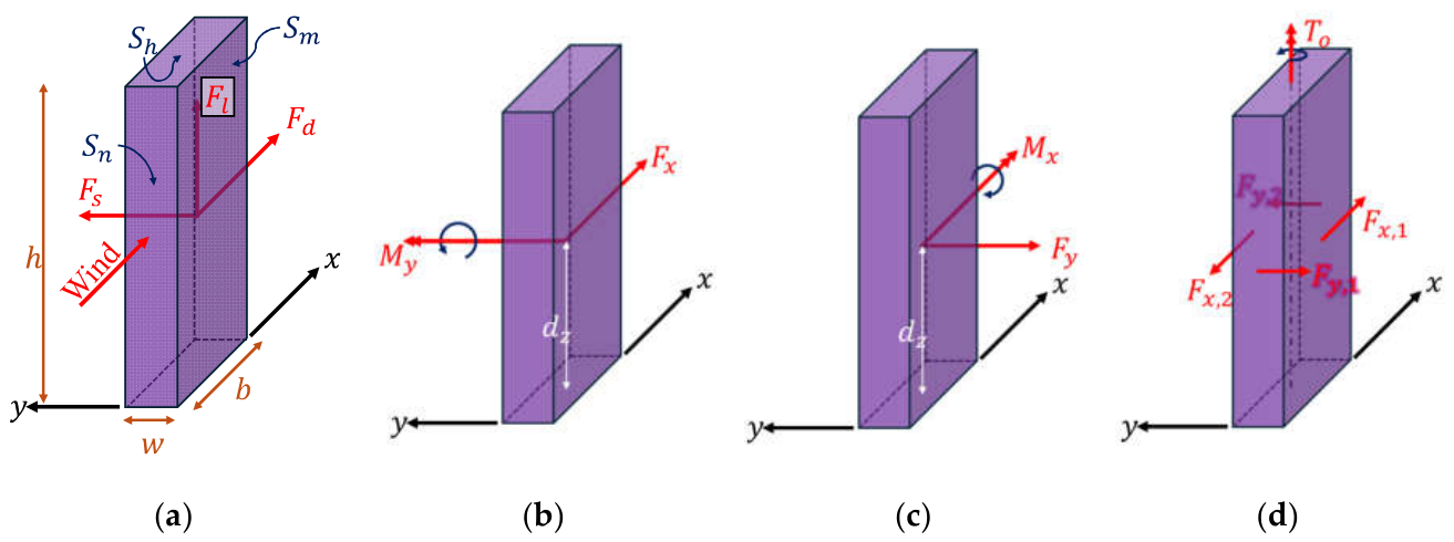
Figure 3.
Simulation domain.
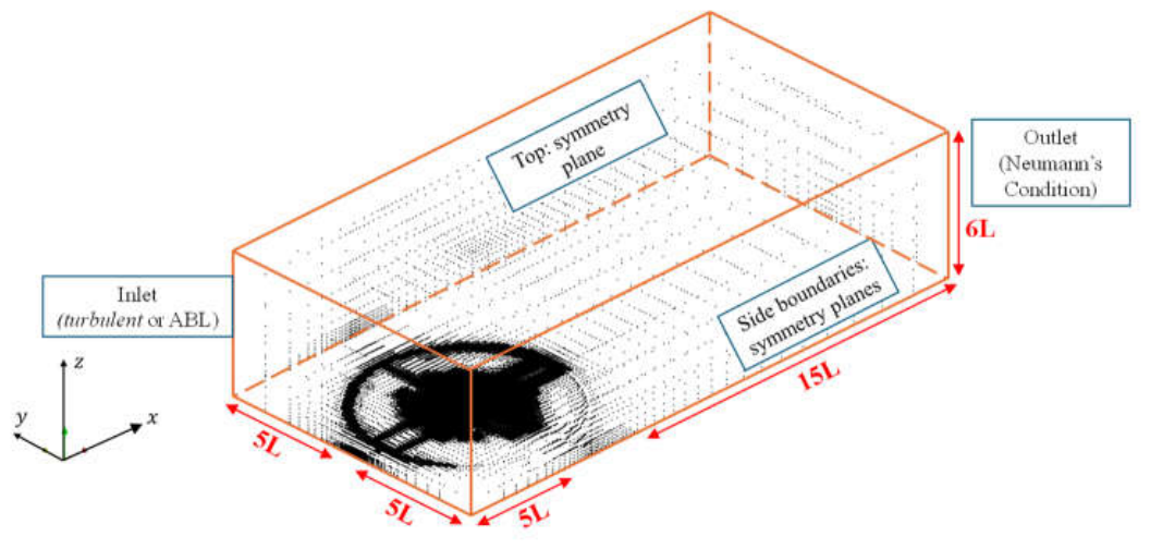
Figure 4.
Mesh detail in the building arrangement: isometric view (a) before and (b) after the CAARC building implementation, and detailed views (c) before and (d) after the insertion of the target structure.
Figure 4.
Mesh detail in the building arrangement: isometric view (a) before and (b) after the CAARC building implementation, and detailed views (c) before and (d) after the insertion of the target structure.
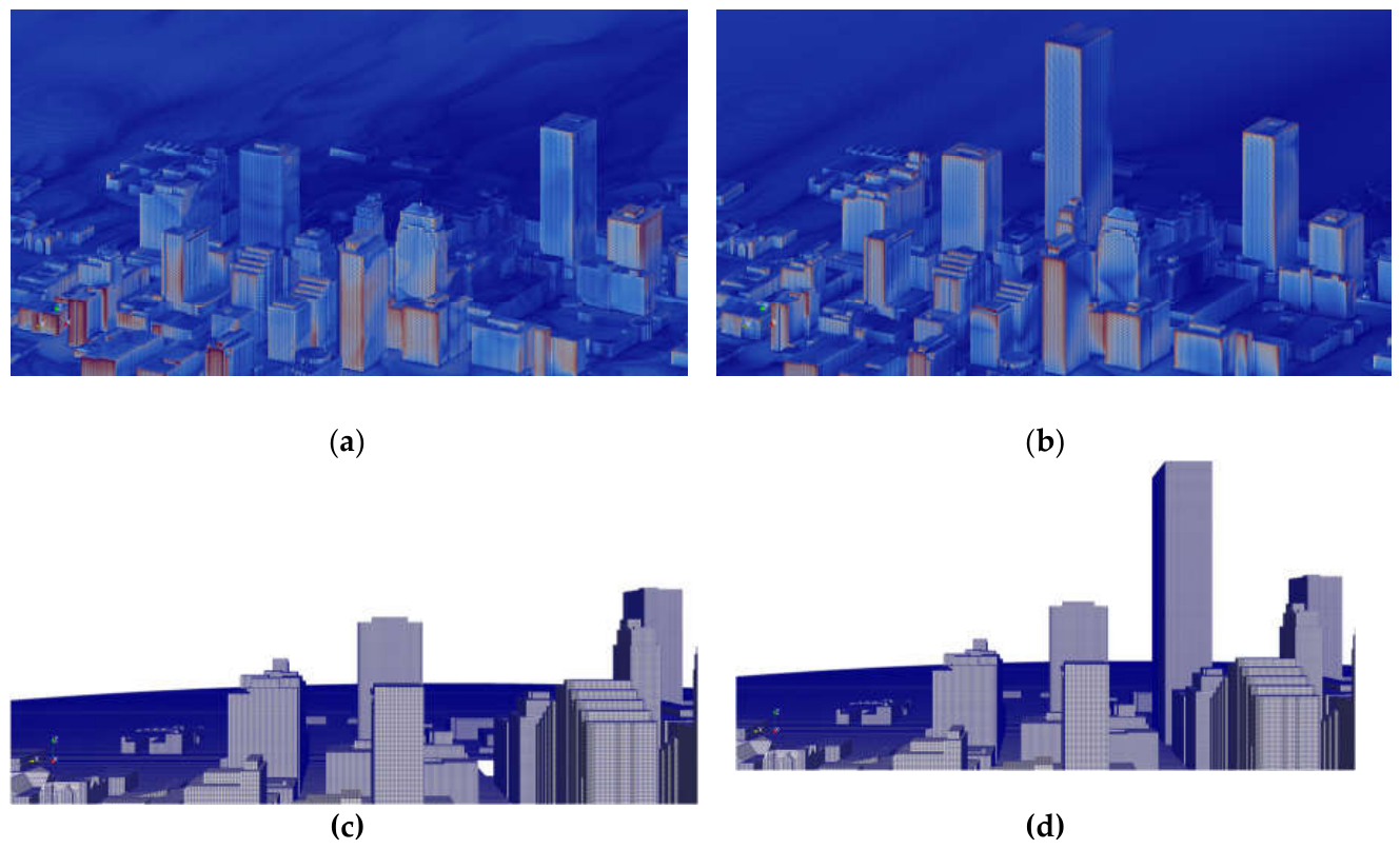
Figure 5.
Michelstadt dataset detailed within M3 level: (a) top and (b) perspective view.
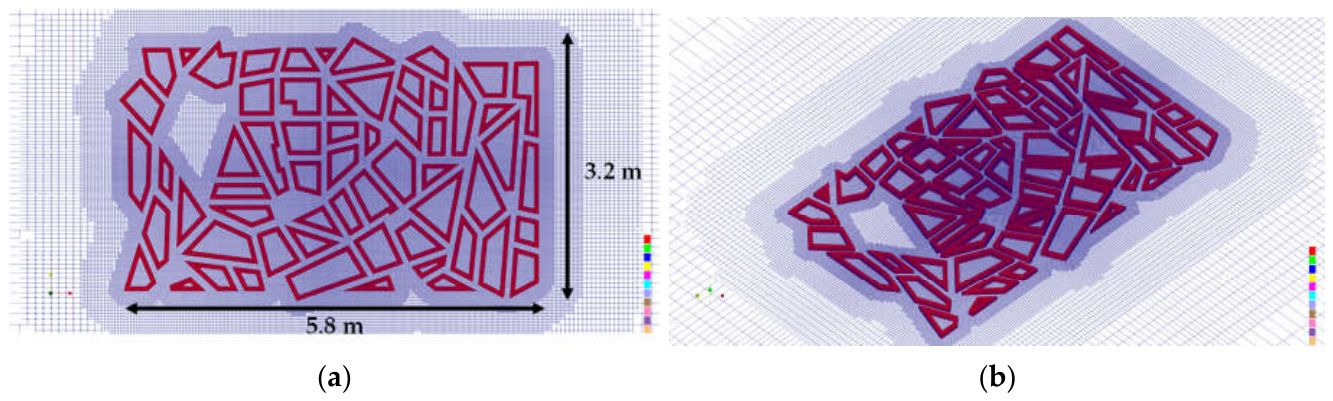
Figure 6.
Analysis threshold of the velocity field: (a) region with the LIDAR detectors from the experimental setup and (b) regions not considered to avoid spurious data.
Figure 6.
Analysis threshold of the velocity field: (a) region with the LIDAR detectors from the experimental setup and (b) regions not considered to avoid spurious data.
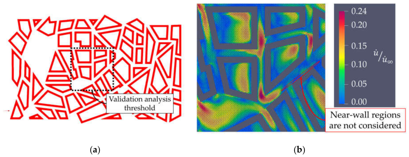
Figure 7.
Refinement detail in near-wall regions within the dataset: (a) M1, (b) M2 and (c) M3.

Figure 8.
Comparative scatter plot for the numerical RANS SST vs. experimental results for (a) M1, (b) M2 and (c) M3.
Figure 8.
Comparative scatter plot for the numerical RANS SST vs. experimental results for (a) M1, (b) M2 and (c) M3.
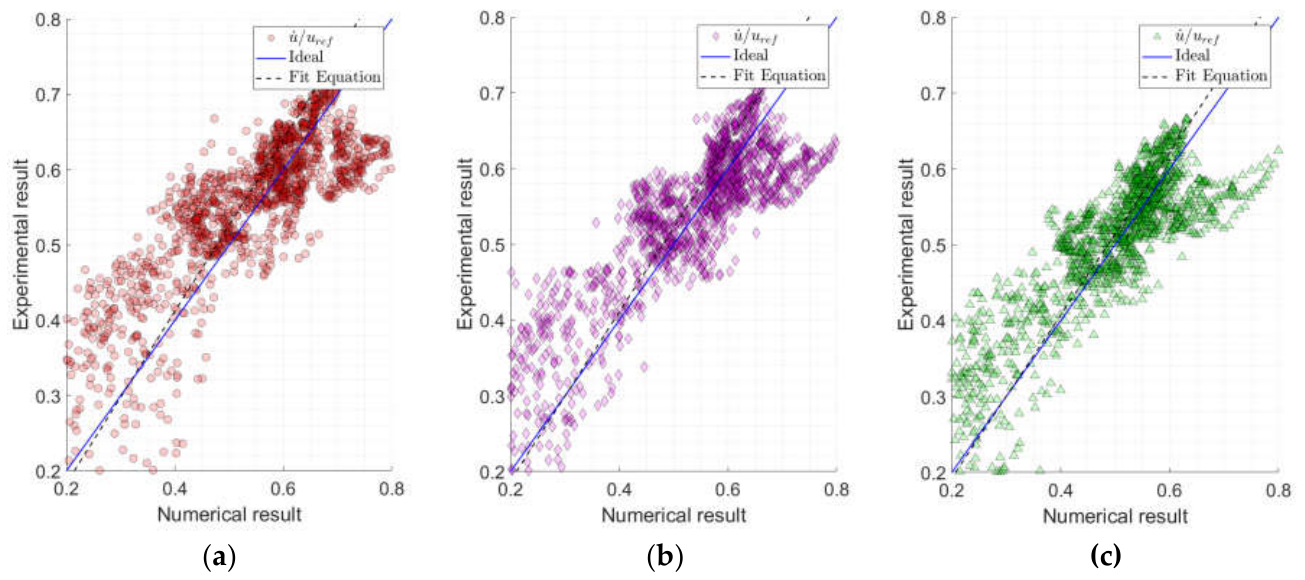
Figure 9.
Comparative scatter plot for the numerical SSTDDES vs. experimental results for (a) M1, (b) M2 and (c) M3.
Figure 9.
Comparative scatter plot for the numerical SSTDDES vs. experimental results for (a) M1, (b) M2 and (c) M3.
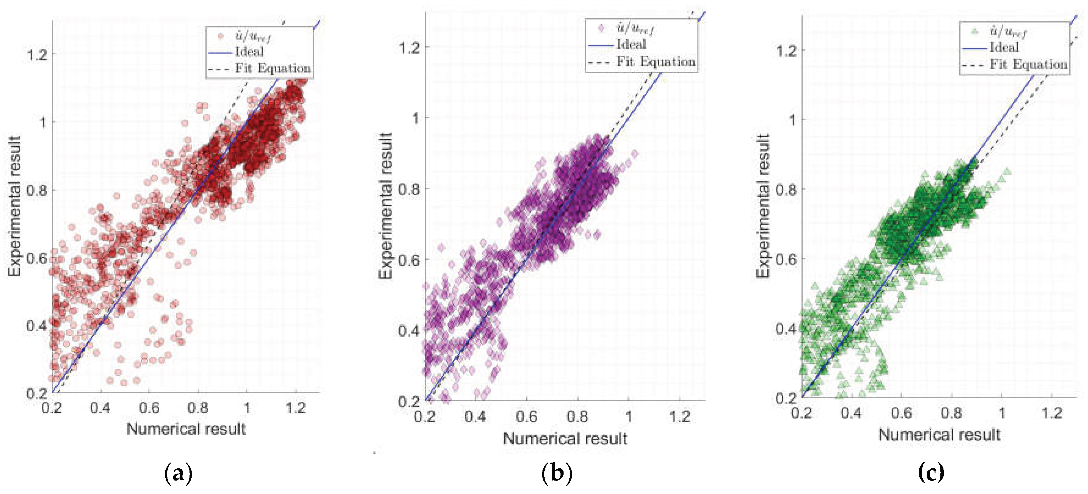
Figure 10.
Analysis of the drag coefficient in both configurations and turbulence models: (a) mean and (b) peak values.
Figure 10.
Analysis of the drag coefficient in both configurations and turbulence models: (a) mean and (b) peak values.
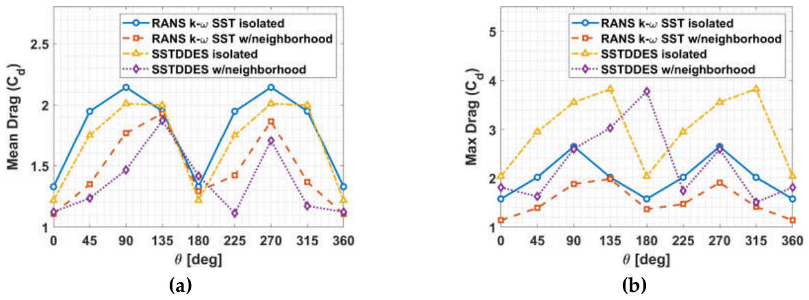
Figure 11.
Analysis of the side forces coefficient in both configurations and turbulence models: (a) mean and (b) peak values.
Figure 11.
Analysis of the side forces coefficient in both configurations and turbulence models: (a) mean and (b) peak values.
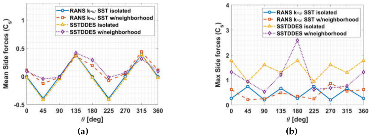
Figure 12.
Analysis of the lift coefficient in both configurations and turbulence models: (a) mean and (b) peak values.
Figure 12.
Analysis of the lift coefficient in both configurations and turbulence models: (a) mean and (b) peak values.
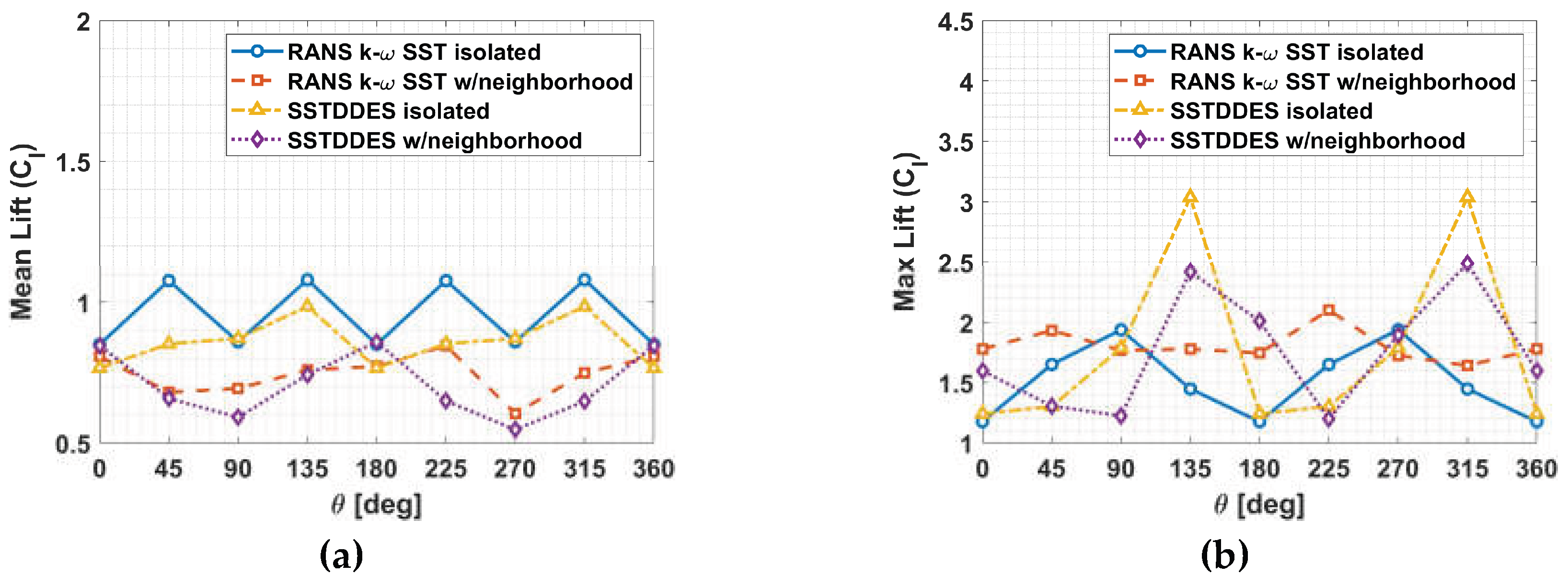
Figure 13.
Analysis of the overturning moment Y coefficient in both configurations and turbulence models: (a) mean and (b) peak values.
Figure 13.
Analysis of the overturning moment Y coefficient in both configurations and turbulence models: (a) mean and (b) peak values.
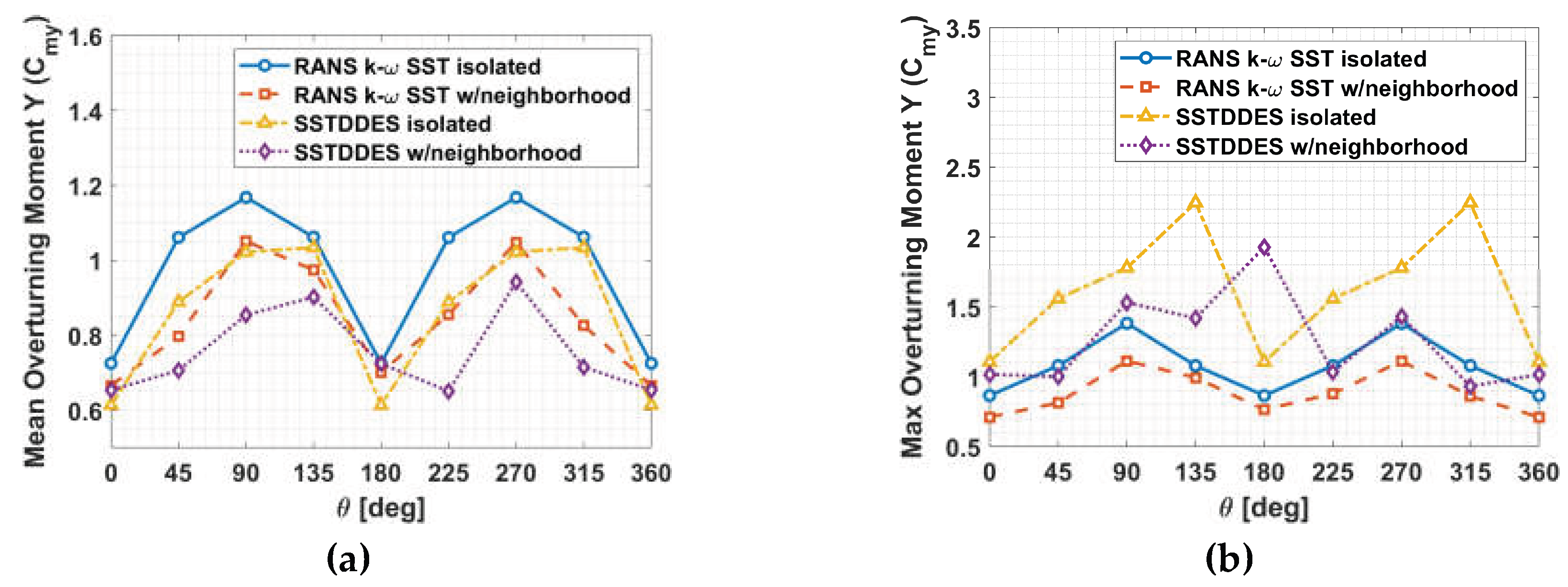
Figure 14.
Analysis of the overturning moment X coefficient in both configurations and turbulence models: (a) mean and (b) peak values.
Figure 14.
Analysis of the overturning moment X coefficient in both configurations and turbulence models: (a) mean and (b) peak values.
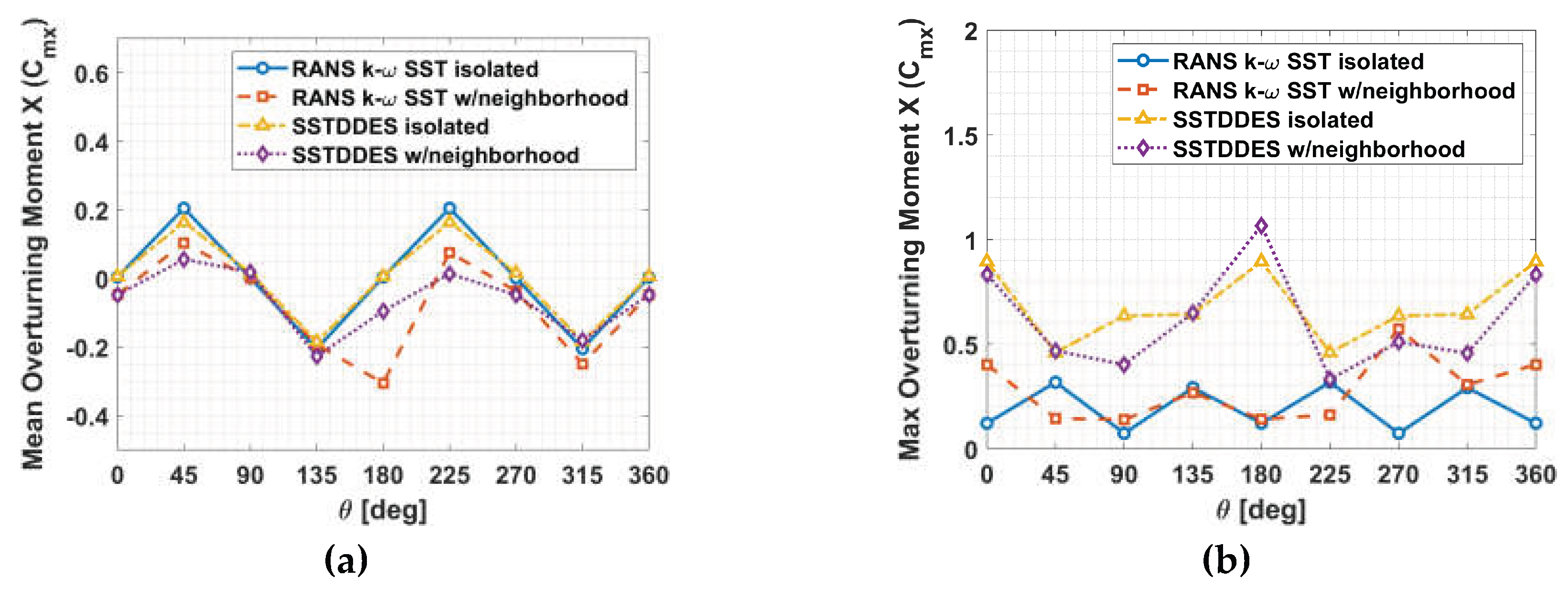
Figure 15.
Analysis of the torsion coefficient in both configurations and turbulence models: (a) mean and (b) peak values.
Figure 15.
Analysis of the torsion coefficient in both configurations and turbulence models: (a) mean and (b) peak values.
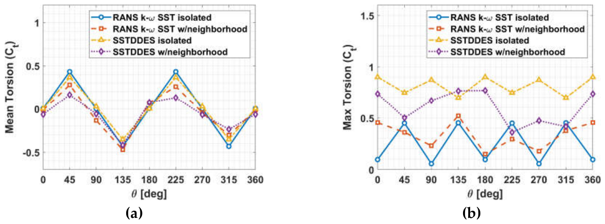
Table 3.
Statistical coefficients and mean values along the simulation for the dimensionless parameter in the Michelstadt dataset using RANS SST model.
Table 3.
Statistical coefficients and mean values along the simulation for the dimensionless parameter in the Michelstadt dataset using RANS SST model.
| Mesh | Time | Fit Equation | R² | FB | FAC2 | RMSE | MAE | |||
|---|---|---|---|---|---|---|---|---|---|---|
| M1 M2 M3 |
0.41 0.68 1.00 |
1.141x – 0.045 1.114x – 0.038 1.073x – 0.022 |
0.970 0.979 0.991 |
0.039 0.030 0.027 |
0.998 0.999 0.999 |
0.087 0.071 0.046 |
0.071 0.058 0.037 |
0.28 0.12 0.05 |
65.10 55.69 47.81 |
10.97 7.98 6.34 |
Table 4.
Statistical coefficients and mean values along the simulation for the dimensionless parameter in the Michelstadt dataset using SSTDDES model.
Table 4.
Statistical coefficients and mean values along the simulation for the dimensionless parameter in the Michelstadt dataset using SSTDDES model.
| Mesh | Time | Fit Equation | R² | FB | FAC2 | RMSE | MAE | |||
|---|---|---|---|---|---|---|---|---|---|---|
| M1 M2 M3 |
15.20 24.01 35.59 |
1.180x – 0.065 1.059x – 0.028 0.944x + 0.011 |
0.958 0.996 0.991 |
0.003 0.036 0.014 |
0.965 0.988 0.975 |
0.105 0.035 0.040 |
0.086 0.025 0.033 |
0.86 0.45 0.25 |
118.78 97.49 87.92 |
21.74 13.79 10.35 |
Disclaimer/Publisher’s Note: The statements, opinions and data contained in all publications are solely those of the individual author(s) and contributor(s) and not of MDPI and/or the editor(s). MDPI and/or the editor(s) disclaim responsibility for any injury to people or property resulting from any ideas, methods, instructions or products referred to in the content. |
© 2026 by the authors. Licensee MDPI, Basel, Switzerland. This article is an open access article distributed under the terms and conditions of the Creative Commons Attribution (CC BY) license.
Copyright: This open access article is published under a Creative Commons CC BY 4.0 license, which permit the free download, distribution, and reuse, provided that the author and preprint are cited in any reuse.