

Submitted:
17 September 2026
Posted:
18 September 2026
You are already at the latest version
Abstract
Controller Area Network (CAN) intrusion detection across vehicles is challenging because identifiers, timing patterns, and payload encodings are vehicle-specific, while serial correlation complicates alarm calibration. This study evaluated target-specific, normal-only adaptation rather than zero-shot transfer. Benchmark labels served only to delimit verified-clean target prefixes; attack labels were excluded from feature construction, model fitting, and calibration. A 12-dimensional residual representation captured per-identifier payload and timing deviations, identifier rarity and novelty, transition surprise, and window-level distributional change. A dependence-informed empirical block-rank (EBR) procedure calibrated Isolation Forest anomaly scores at block level. Across four can-train-and-test target scenarios (five random seeds each), the residual detector achieved an area under the receiver operating characteristic curve (AUROC) of 0.918 (standard deviation (SD) 0.081), an area under the precision–recall curve (AUPRC) of 0.622 (SD 0.372), and a Matthews correlation coefficient (MCC) of 0.573 (SD 0.232). Capture-disjoint and leave-one-capture-out evaluation reduced AUPRC to 0.553 and 0.521, respectively; simultaneous 5% contamination of adaptation and calibration data reduced it to 0.548. At α = 0.05, EBR yielded a block false-positive rate (FPR) of 0.072 and attack-block recall of 0.786, although the merged alarm burden remained 11.1 events per hour. Refitting on ROAD preserved ranking performance (AUROC 0.793; AUPRC 0.503) but produced low and variable alarm recall. These findings support target-specific workflow replication; capture separation, commissioning-data quality, and operating-point selection remain critical for deployment.
Keywords:
controller area network
; automotive cybersecurity
; target-normal adaptation
; normal-only anomaly detection
; Isolation Forest
; alarm calibration
1. Introduction
Modern vehicles depend on continuous communication among electronic control units (ECUs) for powertrain, chassis, body, and advanced driver-assistance functions. Controller Area Network (CAN) remains widely used because of its low cost, priority-based arbitration, reliability, and mature automotive ecosystem [1]. However, CAN was designed for a trusted in-vehicle environment and does not natively provide sender authentication or payload confidentiality. An adversary who gains access through a diagnostic interface, telematics or infotainment system, compromised ECU, or exposed gateway can inject, replay, suppress, or modify syntactically valid frames [2,3,4]. Anomaly-based intrusion detection is therefore attractive for legacy and heterogeneous platforms because it can monitor raw communication without redesigning the underlying protocol.
Existing CAN intrusion detection systems (IDSs) exploit several complementary forms of evidence. Timing- and frequency-based approaches model periodicity, inter-arrival behavior, message counts, and transmission gaps [5,6,7], while related temporal formulations extend these cues [8,9,10]. Payload-oriented and signal-aware methods capture byte- or signal-level manipulations that may preserve nominal transmission rates [11,12,13]. Recent work has also explored signal-level deep models, multimodal and ensemble fusion [14,15,16], knowledge- and graph-based representations [17,18], lightweight image or graph encodings [19,20], and multi-knowledge, adaptive, and physical-layer designs [21,22,23]. Although these advances have improved in-domain accuracy, many evaluations remain tied to a particular vehicle or dataset. High benchmark performance therefore does not necessarily indicate that a learned representation will transfer to vehicles with different identifier assignments, timing scales, payload encodings, and transition structures.
Configuration dependence is especially important when an IDS is deployed across heterogeneous vehicles. The can-train-and-test and ROAD datasets support evaluation across vehicles, attacks, and collection conditions [24,25], while subsequent studies show that capture design and evaluation protocol can materially affect reported IDS performance [26,27]. The official can-train-and-test unknown-vehicle setting withholds the target vehicle from source training. This study deliberately modifies that setting by allowing a trusted, normal-only target commissioning period and therefore evaluates target adaptation rather than zero-shot vehicle transfer. The distinction is operationally important: numerical CAN identifiers and absolute communication statistics can encode vehicle configuration, whereas target-local residuals measure deviations from a vehicle-specific normal reference without requiring labeled target attacks.
A separate deployment challenge arises after an anomaly score has been generated. Recent CAN IDS studies often emphasize discrimination under benchmark-specific thresholds [28,29,30]. Conformal methods provide a principled way to rank nonconformity scores, but their standard finite-sample interpretation relies on exchangeability. Research on prediction beyond exchangeability, time-series conformal inference, and adaptive calibration shows that serial dependence and distribution shift require additional assumptions or adaptive procedures [31,32,33]. In CAN streams, adjacent scores are correlated, and a window-level significance level does not translate directly into block-level performance or operational false-alarm burden. Calibration must therefore specify the testing unit, multiplicity convention, temporal assumptions, and deployment metric.
These observations lead to two related but distinct requirements. First, representation comparability must be separated from attack sensitivity. Vehicle-relative ranks can suppress configuration-specific scale differences but may attenuate sparse local deviations; the primary detector therefore uses target-normal residuals, while behavioral roles are retained for diagnostics and controlled baselines. Second, anomaly ranking must be separated from alarm calibration. The detector is fitted on a trusted target-normal adaptation partition, and a later, disjoint target-normal calibration partition converts the fixed score into block-level alarms. All model estimation and calibration are target specific. Accordingly, heterogeneity in this study refers to repeated evaluation across vehicle datasets, not transfer of learned source-vehicle parameters.
This study makes two contributions. First, it formulates a 12-dimensional target-normal residual representation for normal-only target adaptation. The representation combines robust per-identifier payload and timing deviations, unseen- and rare-identifier ratios, transition and identifier surprise, and window-level changes in the identifier distribution. Vehicle-relative behavioral roles are used to diagnose representation discrepancy rather than to assert vehicle-invariant detection. Second, the study evaluates a dependence-informed empirical block-rank calibration procedure that estimates a candidate temporal scale from target-normal scores, constrains block length to preserve rank resolution, and compares test-block maxima with a disjoint target-normal calibration set. The evaluation separates target-specific ranking, alarm-unit effects, thresholded decision behavior, and operational false-alarm burden. It also includes capture-separated partitions, controlled target-normal contamination, stronger normal-only baselines, and sensitivity analyses of α, event aggregation, and block length. Isolation Forest and empirical ranking are established components; the contribution lies in the residual representation and their controlled integration. Exact calibration validity is not claimed when block exchangeability remains unresolved.
The remainder of this paper is organized as follows. Section 2 defines the target-specific learning setting, residual representation, behavioral diagnostics, empirical block-rank decision rule, and evaluation protocols. Section 3 presents the can-train-and-test results, operational diagnostics, ROAD replication, and robustness and sensitivity analyses. Section 4 discusses the methodological and deployment implications and the principal limitations. Section 5 concludes the paper.
2. Materials and Methods
2.1. Problem Formulation and Overall Framework
Let the chronologically ordered CAN stream from vehicle be , where each frame contains timestamp , CAN identifier , data length , and payload vector . The frame representation is
Model estimation does not use attack labels. Source-domain training uses only normal frames. Trusted target-normal traffic is divided chronologically into an adaptation set and a disjoint calibration set, and the remaining stream is reserved for evaluation. The adaptation set defines target-normal references, fits and standardizes the residual detector, adapts the behavioral baseline, and estimates temporal dependence. The calibration set is used only to construct the empirical alarm-calibration distribution. No attack example or attack-family label is used to define features, fit an anomaly model, select block length, or determine the alarm threshold. In the can-train-and-test experiment, however, ground-truth labels are used before fitting to delimit a verified-clean prefix. Thus, attack-label-free refers to model estimation, whereas the data-selection protocol remains oracle clean and does not represent unsupervised discovery of a clean commissioning interval.
Controlled contamination protocol. Sensitivity to imperfect commissioning data were evaluated at the analysis-window level. At each contamination fraction, randomly sampled target windows overlapping labeled attacks replaced an equal number of nominal windows in the affected adaptation or calibration partition. The substituted windows were then treated as nominal during reference estimation, detector fitting, or calibration, while partition sizes remained fixed. The main sweep contaminated both partitions at 0%, 1%, 3%, 5%, and 10%; a separate location analysis introduced 5% contamination into adaptation only, calibration only, or both. Sampled contamination windows did not overlap the final evaluation blocks. Ground-truth attack overlap was used solely to construct these controlled sensitivity conditions and was not used for feature design, hyperparameter optimization, or threshold selection.
Frames were segmented into non-overlapping fixed-duration windows of length , and windows with fewer than frames were discarded. The workflow then proceeded in three stages. First, a vehicle-relative behavioral representation was constructed for transfer analysis and controlled baselines, while a target-normal residual representation preserved local anomaly evidence. Second, a target-residual Isolation Forest (IF) generated the primary anomaly score; behavioral-only and role-plus-residual models were retained as prespecified sensitivity analyses. Third, a dependence-informed block-maximum calibration layer converted the fixed residual score into alarms using only .
2.2. Behavioral Diagnostics and Target-Normal Residual Scoring
Behavioral-role representation. The same numerical CAN identifier need not represent the same function across vehicles. Each identifier was therefore characterized by an eight-dimensional normal-traffic signature comprising transmission frequency , median same-ID inter-arrival time , coefficient of variation , normalized payload entropy , bit-flip rate , transition entropy , and normalized transition-graph in- and out-degrees and :
Because absolute signature values remain vehicle dependent, each dimension was converted to a within-vehicle rank. For signature dimension , the resulting role coordinate is
For each window , the behavioral representation aggregated frame-level role vectors using component-wise mean, 90th percentile, and standard deviation, together with the fraction of reference identifiers active in the window. With denoting the role vector of frame and the active identifier set, the window representation is
Target-normal residual representation. Behavioral normalization can improve comparability while attenuating sparse local deviations. A separate target-local reference was therefore constructed using only . For payload byte of identifier , the normal center and scale were estimated by the median and median absolute deviation (MAD), with a floor for nearly constant bytes:
Frame-level payload and inter-arrival residuals were defined by robust standardized deviations. The empirical target-normal identifier probability and transition probability additionally defined identifier- and transition-surprise terms. Residual magnitudes were clipped at 12; identifiers absent from received a fixed penalty of 8; and the bottom 20% of positive target-normal identifier probabilities defined the rare-ID set. For frame , the principal residual quantities are
Residual implementation. Equation (5) defines the payload center and scale; the superscript x used in Equation (6) is omitted here for compactness. Analogous centers and scales were estimated from same-identifier inter-arrival times and denoted by the superscript Delta. Zero-probability identifier or transition events were assigned the fixed unseen-event penalty before logarithmic scoring, which avoids undefined log-zero values. Numerical scale floors, the smoothing convention, payload-byte aggregation, and capture-boundary handling are fixed implementation parameters and were applied uniformly across the reported experiments.
Each residual window combined the unseen-ID and rare-ID ratios; mean, upper-quantile, and maximum payload deviations; mean and upper-quantile timing deviations; transition- and identifier-surprise statistics; and the total-variation distance between the window identifier distribution and the target-normal distribution . The implemented 12-dimensional residual vector is
One-class scoring. Isolation Forest serves as a lightweight normality estimator rather than a methodological contribution. The primary residual model was trained only on target-adaptation residual vectors and contained 100 trees with at most 256 observations per learner. Before fitting, each residual feature was robustly standardized using the median and MAD estimated from the target-adaptation residual vectors, as defined in Equation (8). The anomaly score returned by the fitted forest was then used directly for calibration. A transfer-oriented behavioral IF was trained on source behavioral windows and target-adaptation behavioral windows, with source windows subsampled at a fixed 1:4 source-to-target ratio. The one-class support vector machine (OCSVM) and local outlier factor (LOF) used the same target-adapted behavioral input after identical robust standardization, thereby providing detector baselines under a controlled representation.
Comparator implementation. All comparisons used identical target-normal information boundaries, evaluation windows, and block construction. The behavioral IF, OCSVM, and LOF baselines used the same standardized behavioral input. Neural baselines were trained only on target-normal adaptation data, produced one scalar anomaly score per evaluation window, and used the same target-normal calibration partitions and block-level decision layer as the residual IF. Attack labels were not used for optimization. The common pipeline settings are summarized in Table 1.
The MLP-AE used a symmetric 12-32-8-32-12 encoder-decoder with rectified linear unit (ReLU) hidden units and a linear output. The LSTM-AE processed sequences of 16 residual windows with encoder widths of 64 and 32, a mirrored decoder, and dropout of 0.20. Deep SVDD used a bias-free 12-32-16-8 embedding and a one-class center objective. The TCN-AE used 16-window sequences, three causal residual blocks with 32, 64, and 64 channels, a kernel size of 3, dilations of 1, 2, and 4, and a 16-dimensional latent code. The autoencoders used mean squared reconstruction error, Adam with a learning rate of 0.001, a batch size of 64, a maximum of 100 epochs, and early stopping with a patience of 10 epochs. Deep SVDD used Adam with a learning rate of 0.0001, a batch size of 128, and 150 epochs. Reconstruction error or squared distance from the Deep SVDD center defined the window score. These settings follow representative normal-only CAN and time-series designs [34,35,36] and were applied consistently across the reported comparisons. Hyperparameters were selected a priori from these reference designs and held fixed across scenarios; no hyperparameter was tuned on evaluation data or with attack labels.
Behavioral-only and hybrid analyses were retained to determine whether source-derived behavioral information adds evidence beyond target-local residuals. In the hybrid sensitivity analysis, behavioral and residual scores were standardized separately using target-normal adaptation scores and combined by a predefined maximum rule. The rule was not optimized with attack labels. For all method comparisons, block length was derived from the fixed primary residual score so that scoring effects are not conflated with calibration effects.
2.3. Dependence-Informed Empirical Block-Rank Calibration, Decision Rules, and Experimental Protocol
Dependence-informed calibration. Consecutive CAN windows can remain dependent even when they do not overlap. The sample autocorrelation function (ACF) of target-residual adaptation scores was therefore estimated within capture boundaries. Starting from 80 lags, the inspected range was extended in steps of 40 up to 240 lags whenever the current tail remained unresolved. The candidate length was the first lag of a run of eight consecutive autocorrelations falling within the approximate 95% sampling band; if no such run was observed, the candidate was set immediately after the last significant lag within the inspected range. Because an excessively large block would reduce empirical rank resolution, the operational length was further constrained to retain at least 100 normal calibration blocks whenever feasible:
Here, the capture-specific calibration-window counts determine the largest block length that retains the required rank resolution. The minimum of 100 blocks was chosen because the smallest evaluated significance level, α = 0.01, requires approximately 100 calibration blocks to resolve an upper-tail rank near that level. Calibration scores were partitioned into non-overlapping blocks within capture boundaries, and each block was represented by its maximum anomaly score. For calibration block j,
For a test block with maximum score S*, Equation (11) defines a smoothed upper-tail empirical rank statistic by counting calibration-block maxima at least as large as S*. A block is declared positive when that statistic does not exceed α:
The default operating point was α = 0.05, and {0.01, 0.025, 0.05, 0.075, 0.10} was used to examine calibration across operating levels. Under exchangeable blocks, the statistic in Equation (11) has the usual finite-sample conformal interpretation. In the present CAN setting, however, blocking is only a dependence-reduction heuristic; exact validity is not claimed when long-range autocorrelation remains unresolved or operating conditions drift. The rule is therefore referred to as empirical block-rank (EBR) calibration; realized FPR, attack-block recall, block-length diagnostics, and benign-condition shift are reported, and the rank is not interpreted as a calibrated p-value.
Evaluation unit and block labeling. All block-level decision metrics used the same non-overlapping test blocks of operational length b. A block was labeled positive when at least one constituent evaluation window overlapped a labeled attack interval; blocks containing only benign windows formed the FPR denominator. The final incomplete block in each capture was discarded, and blocks never crossed capture boundaries. Threshold-free block metrics used the block-maximum score, whereas MCC used the default α = 0.05 decision rule. Window rules were mapped to the same block-level reporting unit only in explicitly labeled descriptive comparisons.
Comparator decision rules. Window Percentile applied the empirical 1 − α quantile of calibration-window scores to individual test windows and mapped the resulting decisions to a block alarm using an any-window rule. Window empirical rank (Window ER) replaced the percentile threshold with the same upper-tail rank construction at the window level and used the same any-window mapping. Bonferroni empirical rank (Bonferroni ER) tested each constituent window at α/b before applying the any-window rule. ACF-Block Percentile applied an empirical 1 − α quantile to calibration-block maxima, whereas EBR applied Equation (11) directly to the test-block maximum. These rules share the same anomaly score but not the same primitive testing unit; comparisons involving window rules therefore combine within-block multiplicity with temporal and distributional dependence.
Interpretive scope. The block procedure is dependence-informed, not dependence-eliminating. When the operational block length was shortened by the calibration-resolution constraint or the ACF tail remained unresolved, block exchangeability was not established and the empirical tail ranks did not provide exact finite-sample FPR control. EBR was therefore described as a block-maximum calibration heuristic, and its results were reported as descriptive operating characteristics together with block length, rank resolution, and benign-condition shift.
Can-train-and-test protocol. The principal evaluation used the four official can-train-and-test sets [24]. Each set contributed its test_04_unknown_vehicle_unknown_attack subset, but the present protocol departed from the official zero-shot interpretation by observing target-normal data. The four scenarios were Chevrolet Impala/Chevrolet Silverado, Chevrolet Traverse/Subaru Forester, Chevrolet Silverado/Subaru Forester, and Subaru Forester/Chevrolet Traverse; the first name denotes the official source vehicle and the second the target. Frames labeled as attacks in the source data were removed. For each target capture, benchmark labels delimited the prefix preceding the first labeled attack; 40% of this verified-clean prefix was reserved as oracle-clean target-normal traffic. The first chronological half was assigned to adaptation and the second to calibration, while the remaining stream was reserved for evaluation. Adaptation and calibration were temporally disjoint but not capture-level disjoint. Five random seeds were used to vary source subsampling and Isolation Forest construction. The principal estimate therefore represents a within-capture temporal holdout under oracle-clean target adaptation, not fixed-model unknown-vehicle transfer. Capture separation and controlled target-normal contamination were evaluated separately as robustness analyses in Section 3.5.
ROAD protocol. The same feature specification, detector settings, block-selection rule, and alarm levels were applied to ROAD [25], but the target-normal references and residual detector were refitted using ROAD normal files. Five file-level splits rotated the available normal files through adaptation, calibration, and benign evaluation roles while reusing a limited pool of attack captures. The splits therefore assessed workflow reproducibility after target-specific refitting on a single vehicle; they are overlapping resamples rather than independent external cohorts. Four accelerator post-exploit captures were summarized separately because they represent vehicle-state effects rather than labeled injected-frame intervals.
The area under the receiver operating characteristic curve (AUROC) and the area under the precision-recall curve (AUPRC) summarized the ranking performance of block-maximum scores. Within each scenario, AUPRC lift was calculated as AUPRC divided by attack-block prevalence before aggregation across scenarios. The Matthews correlation coefficient (MCC), empirical block false-positive rate (FPR), and attack-block recall were calculated at the default operating level of α = 0.05. For can-train-and-test analyses, random seeds were first averaged within each physical scenario, after which the mean and standard deviation were calculated across the four scenario means. ROAD summaries are reported as mean (SD) across five file-level splits. The capture-separation, normal-only baseline, contamination, operating-level, event-processing, and block-length analyses used the same information boundaries and aggregation logic. The analyses report scenario-aggregated point estimates and sensitivity curves; because only four vehicle scenarios were available, the comparisons are interpreted descriptively rather than as population-level hypothesis tests.
The robustness and sensitivity analyses included contamination levels of 0%, 1%, 3%, 5%, and 10%; same-capture chronological, capture-disjoint, and leave-one-capture-out partitions; MLP-AE, LSTM-AE, Deep SVDD, and TCN-AE normal-only baselines; an α sweep over {0.01, 0.025, 0.05, 0.075, 0.10} with alarm-merging and refractory comparisons; and block lengths of {16, 32, 48, 64, 96} windows. The same-capture condition was the principal chronological split defined above. In the capture-disjoint condition, complete target captures were assigned to commissioning or evaluation so that no capture contributed to both. In leave-one-capture-out evaluation, each available target capture was held out once, while the remaining target captures provided adaptation and calibration data. Held-out predictions were aggregated at the target-scenario level before the four-scenario summary was calculated.
All estimators used the same target-normal information boundary and the same evaluation and calibration units. Each neural model was trained without attack examples, returned a scalar anomaly score for each evaluation window, and was assessed through the common block-maximum protocol. Fixed settings were retained across scenarios. The comparison therefore evaluated sensitivity to estimator family under a matched protocol and was not interpreted as evidence of architectural optimality.
With M = 100 calibration blocks, the smallest attainable smoothed empirical rank is 1/(M + 1) = 0.0099; α values below 0.01 were therefore excluded. At α = 0.05, event postprocessing compared no merging with merge/refractory settings of 5/15 s, 10/30 s, and 20/60 s. The five block lengths correspond to durations of 0.8, 1.6, 2.4, 3.2, and 4.8 s at a window duration of 0.05 s. These finite grids were used for sensitivity analysis rather than optimization with attack labels.
3. Results
3.1. Target-Adaptive Detection and Representation Diagnostics
Across four can-train-and-test target-adaptation scenarios, the primary target-residual IF achieved an AUROC of 0.918 (SD 0.081), an AUPRC of 0.622 (SD 0.372), an AUPRC lift of 7.805 (SD 2.962), and an MCC of 0.573 (SD 0.232) after hierarchical aggregation across scenarios and random seeds. Scenario-level AUPRC ranged from 0.210 for Traverse/Forester to 0.962 for Forester/Traverse, while attack-block prevalence ranged from approximately 0.027 to 0.251. These results describe performance after fitting a target-specific normal model; they do not measure zero-shot source-to-target parameter transfer. Reporting AUPRC lift alongside raw AUPRC helps distinguish prevalence effects from ranking quality, but the wide SD indicates substantial scenario heterogeneity. Figure 1 presents the scenario-level results and provides the context needed to interpret the aggregate metrics alongside their between-scenario dispersion.
Figure 1 shows high AUROC in all four scenarios but substantial variation in AUPRC and MCC. The contrast is clearest for Traverse/Forester: AUROC remained 0.896, whereas AUPRC fell to 0.210; by comparison, Silverado/Forester and Forester/Traverse achieved AUPRC values of 0.909 and 0.962, respectively. MCC did not vary monotonically with AUPRC, indicating that thresholded decision quality depends on score overlap and the selected operating point rather than ranking alone. Because the primary residual model does not use source data, the source/target labels denote official dataset pairings rather than learned source contributions. Differences in target capture, attack composition, and prevalence remain plausible explanations for the between-scenario variation. Table 2 summarizes the implemented baselines and decision rules; the matched analyses in Section 3.3 separate the effects of target adaptation, residual representation, and detector family.
As shown in Table 2, the target-residual IF achieved the highest mean ranking performance and default-threshold MCC among the implemented configurations, with an AUPRC of 0.622 and an MCC of 0.573. The target-adapted behavioral IF and OCSVM were weaker on average, and the fixed hybrid score did not improve on residual-only detection. The matched target-normal raw-feature baseline, residual detector-family comparison, and feature-group ablations in Section 3.3 further isolate the contribution of the residual representation from target adaptation and estimator choice. Figure 2 compares raw identifier signatures with behavioral-role signatures across the same four vehicle pairings.
Figure 2 shows that within-vehicle ranking reduced the standardized squared radial basis function (RBF)-kernel maximum mean discrepancy (MMD) by 81.7–98.2% across scenarios, with a mean reduction of 91.2%. The largest raw discrepancy, 0.203 for Impala/Silverado, decreased to 0.004 after role normalization. The Silverado/Forester discrepancy similarly decreased from 0.104 to 0.006, while the already smaller Forester/Traverse discrepancy decreased from 0.048 to 0.009. The reduction was therefore greatest where raw identifier signatures were most vehicle specific. Because marginal rank normalization is designed to equalize scale, however, this result is best interpreted as a representation diagnostic rather than evidence of invariant detector inputs. Both raw and role-window domain classifiers remained almost perfectly discriminative, demonstrating that vehicle identity persisted at the complete-window level. Figure 3 therefore examines attack-family behavior and adaptation budget without assuming that behavioral ranks form a transferable anomaly detector.
Figure 3a shows that the residual branch achieved the highest or joint-highest mean AUPRC for every displayed attack family. Relative to the target-adapted role IF, AUPRC increased from 0.40 to 0.68 for combined spoofing and from 0.23 to 0.61 for speed spoofing, whereas the improvement for gear spoofing was only from 0.02 to 0.11. The largest gains therefore occurred for attacks that produced conspicuous payload or timing residuals, while subtle gear and RPM manipulations remained difficult. Figure 3b shows limited change in mean residual AUPRC as the target-normal adaptation fraction decreased, including an AUPRC of 0.580 at the 5% budget. The between-scenario error bars were much larger than the change in the mean curve, so the result supports robustness to adaptation budget only within the evaluated range, not budget invariance. Because absolute duration, window count, and identifier coverage vary by capture, the percentage-budget result does not establish an absolute minimum commissioning requirement. Figure 4 compares detector choice and attack-label-free fusion under the adapted-role setting.
Figure 4a shows that OCSVM and Isolation Forest performed similarly on adapted-role inputs. OCSVM achieved the higher mean AUPRC (0.492 versus 0.456), whereas Isolation Forest achieved the slightly higher MCC (0.438 versus 0.427); the wide, overlapping dispersions do not support a decisive ranking. LOF was consistently weaker, with a mean AUPRC of 0.202 and an MCC of 0.079. Figure 4b shows only modest differences among the fixed max-z, mean-z, and empirical cumulative distribution function (ECDF)-mean fusion rules, whose AUPRC values were 0.561, 0.569, and 0.529, respectively; none exceeded the residual-only mean AUPRC of 0.622. Detector and fusion choices therefore had a smaller effect than the choice of representation. The matched residual-input analysis in Section 3.3 tests this interpretation while holding the learning setting constant.
3.2. Block-Length Selection and Decision-Rule Comparison
The ACF-based candidate length frequently exceeded the block size supported by the available calibration data. Across 20 scenario-seed runs, the median operational block length was 48 windows (2.4 s). The calibration-resolution constraint was active in all 20 runs, and the ACF tail remained unresolved at the maximum inspected lag in 10 runs. The implemented block lengths therefore balance the estimated dependence scale against finite calibration resolution; they do not establish independence or exchangeability of the block maxima. Figure 5 shows the resulting scenario-specific block lengths and corresponding durations.
Figure 5 shows that scenario-specific operational block lengths ranged from 27 windows (1.35 s) for Silverado/Forester to 94 windows (4.70 s) for Impala/Silverado, with intermediate values of 44 and 52 windows. The longest block was approximately 3.5 times the shortest. A single global block length would therefore either truncate the estimated dependence scale in some scenarios or unnecessarily delay decisions in others. Longer blocks also reduce the number of calibration maxima available for threshold estimation, exposing a direct tradeoff among dependence coverage, calibration resolution, and detection delay. Because the resolution constraint was active in every run, the displayed lengths should not be interpreted as fully resolved empirical dependence horizons. Figure 6 compares the five decision rules after mapping them to a common block-level reporting unit.
After window-level decisions were mapped to block alarms, Window Percentile and Window ER produced block FPRs of 0.668 and 0.665, respectively, with recall of 0.981 for both. These FPRs exceeded the nominal 0.05 level by more than a factor of 13, showing that an any-window block alarm achieved high recall only at an unacceptable false-alarm cost. Bonferroni ER reduced FPR to 0.053 but also reduced recall to 0.605. ACF-Block Percentile and EBR retained higher recalls of 0.794 and 0.786 while reducing FPR to 0.080 and 0.072, respectively. The small difference between the two block-maximum rules suggests that redefining the testing unit accounts for most of the improvement, while empirical ranking provides a smaller refinement. The matched-FPR analysis in Section 3.3 separates this decision-granularity effect from the calibration rule.
Operational interpretation. The reported FPR is the fraction of benign blocks declared positive, not an alarm-event rate. At the median block duration of 2.4 s, this aggregate block FPR corresponds to approximately 108 alarm-positive blocks per hour under continuous assessment. After adjacent positive blocks were merged within 10 s and a 30 s refractory interval was applied, the pooled rate decreased to 11.1 alarm events per hour. Event aggregation therefore reduced repeated alarms, but the remaining burden was still too high for unsuppressed deployment. Mean feature-construction, scoring, and calibration times were 772.7 s, 35.6 s, and 0.038 s, respectively, corresponding to 9,222 frames/s in the reported batch environment. These throughput measurements exclude hardware-specific memory use and end-to-end online latency and therefore do not establish real-time deployment readiness.
3.3. Matched Baselines, Feature Ablations, and Block-Level Comparison
Matched comparisons indicated that target-normal adaptation contributed more than the choice among the evaluated one-class estimators. The target-normal raw-feature IF outperformed the zero-shot source-normal residual model, and the full target-residual representation increased AUPRC from 0.505 to 0.622. On the same residual inputs, OCSVM and LOF approached but did not match the primary IF. The detector and ablation results in Figure 7 therefore support a representation-driven interpretation rather than a claim of IF-specific superiority.
Across the four scenario-level paired comparisons, target-residual IF exceeded target-normal raw-feature IF by 0.039 in AUROC, 0.117 in AUPRC, and 0.101 in MCC. By contrast, the AUPRC difference between residual IF and residual OCSVM was 0.035. These values are descriptive paired differences across the observed scenarios, not population-level hypothesis tests. Figure 7b shows a coherent ablation ordering: removing payload residuals caused the largest AUPRC decrease (−0.074), followed by retaining only maximum and mean summaries (−0.065), removing transition and surprise features (−0.056), removing identifier-rarity and distribution-shift features (−0.039), and removing timing features (−0.027). The full representation performed best on every displayed metric, indicating that payload information made the largest individual contribution while the remaining feature groups provided complementary rather than redundant information.
A retrospective matched-FPR analysis substantially reduced the apparent advantage associated with changing the test unit. Thresholds were aligned post hoc to an empirical evaluation-set benign block-FPR target near 0.05. They were used only to compare ranking and decision granularity and are not deployable calibration rules. Under this matched condition, EBR achieved a recall of 0.760, compared with 0.742 for Window Percentile, 0.748 for Window ER, and 0.751 for ACF-Block Percentile. The difference from the non-rank block-maximum rule was small, whereas the window rules alarmed earlier because they acted before block completion. Figure 8 reports the point estimates and descriptive error bars for all four decision metrics.
Figure 8a–c shows that all five retrospectively matched methods operated within a narrow block-FPR range of 0.049–0.053, allowing recall and MCC to be compared without the large false-alarm imbalance in Figure 6. EBR had the highest point estimates for recall (0.760) and MCC (0.572), but its recall advantage over ACF-Block Percentile was only 0.009. Figure 8d shows the associated timing cost: the two window rules had median latencies near 1.1 s, whereas EBR waited approximately 2.4 s for block completion; Bonferroni ER was the slowest, at 2.85 s. This latency penalty is operationally material. Most of the improvement over the original window-wise rules is therefore attributable to testing and calibrating block maxima, with empirical ranking providing only a small additional benefit.
3.4. Scenario Heterogeneity, Operational Burden, and ROAD Replication
The descriptive, capture-respecting uncertainty intervals preserved the separation between the stronger Silverado/Forester and Forester/Traverse scenarios and the more difficult Traverse/Forester scenario. Because only four vehicle scenarios were available, the intervals display within-dataset uncertainty and do not support population-level inference about cross-vehicle performance. Figure 9 presents this heterogeneity directly.
Across the three panels of Figure 9, the two strongest scenarios were Silverado/Forester (AUROC 0.977, AUPRC 0.909, MCC 0.788) and Forester/Traverse (AUROC 0.986, AUPRC 0.962, MCC 0.743). By contrast, Traverse/Forester retained an AUROC of 0.896 but had an AUPRC of 0.210, demonstrating that favorable ranking can coexist with weak precision under scenario-specific prevalence and score overlap. The aggregate estimates fell between these markedly different regimes, and their intervals did not obscure the separation. Reporting only aggregate AUROC or AUPRC would therefore conceal the main generalization result: performance was high for two vehicle pairings but remained fragile in at least one target setting.
Even after event merging, the false-alarm rate ranged from 5.6 to 16.1 events per hour and remained too high for unsuppressed deployment. Benign-state average run length ranged from 19.0 to 83.9 s, while median detection delay followed the scenario-specific block duration. Figure 10 illustrates the practical benefit of block calibration while also showing that the α = 0.05 operating point was not deployment ready.
Figure 10a shows that empirical block FPR varied from 0.056 to 0.093 across scenarios, with Traverse/Forester farthest above the nominal 0.05 level. In Figure 10b, Silverado/Forester produced the largest raw and merged burden (189.3 positive blocks and 16.1 alarm events per hour), whereas Impala/Silverado produced 42.9 positive blocks and 5.6 events per hour. Figure 10c shows the expected inverse relationship between false alarms and benign-state average run length, which ranged from 19.0 to 83.9 s. Figure 10d further indicates that scenarios with longer blocks tended to incur longer median detection delays. Event merging reduced repeated alarms by approximately an order of magnitude in the pooled result, but it did not produce a deployment-ready operating point because alarm burden and delay remained scenario dependent.
Split-level ROAD results showed that aggregate recall and FPR were driven primarily by one split. The first three splits produced zero recall and zero FPR; the fourth yielded a recall of 0.014 and an FPR of 0.011; and the fifth combined a recall of 0.571 with an FPR of 0.249. Figure 11 makes this instability explicit and prevents the five overlapping splits from being interpreted as independent external cohorts.
Figure 11a shows AUROC, AUPRC, and MCC increasing from 0.683, 0.246, and −0.113 in split 1 to 0.903, 0.760, and 0.227 in split 5. Because split number is only a file-partition label, this visual trend does not indicate progressive learning. Figure 11b explains the instability of the aggregate alarm metrics: splits 1–3 generated no positive attack or benign blocks, split 4 remained near zero, and split 5 alone accounted for the observed recall and FPR. The same split contributed most detections and most false alarms; averaging the five overlapping partitions therefore obscures dependence on the selected normal-refitting and calibration files.
A separate exploratory capture-level analysis compared four accelerator post-exploit captures with ten ambient controls. Three captures had clearly elevated median standardized scores and positive-block fractions, whereas Accelerator A3 was intermediate. Because no independently validated capture-level decision threshold was specified and only four attack captures were available, Figure 12 is interpreted descriptively rather than as an estimate of sensitivity or specificity.
Figure 12 shows elevated values for Accelerator A1, A2, and A4, with median standardized scores of 3.21, 2.64, and 3.87 and positive-block fractions of 0.184, 0.129, and 0.231, respectively. Accelerator A3 had a lower score of 1.42 and a positive-block fraction of 0.041, although both remained above the ambient-control means of 0.61 and 0.018. This descriptive gradient indicates that the post-exploit state contained anomaly evidence of varying strength. It does not support a capture-level sensitivity or specificity claim without a predefined threshold and a larger, independent set of attack and ambient captures.
The fixed analysis procedure was applied to ROAD without reselecting the feature specification, but the residual reference and detector were refitted using ROAD normal files. The experiment therefore evaluates cross-dataset workflow replication after target-specific refitting rather than transportability of a fixed trained model. Across five overlapping file-level splits, the target-residual IF achieved an AUROC of 0.793 (SD 0.087), an AUPRC of 0.503 (SD 0.203), and an AUPRC lift of 1.905 (SD 0.391). At α = 0.05, however, MCC was 0.057 (SD 0.134), attack-block recall was 0.117 (SD 0.254), and block FPR was 0.052 (SD 0.110). The mean FPR alone therefore does not demonstrate stable calibration. Table 3 summarizes the implemented ROAD configurations.
Table 3 shows that the target-refitted residual detector achieved the highest mean AUROC and AUPRC among the implemented ROAD configurations. Nevertheless, its low mean MCC and recall, together with standard deviations larger than the corresponding means, indicate unstable alarm power across file splits. Because the five splits reuse a small pool of normal files and the same attack captures, they are not independent external cohorts. The evidence therefore supports reproducibility of the workflow on a second dataset more strongly than operational generalization. Figure 13 compares the target-refitted configurations and decomposes the primary result by ROAD attack family.
Figure 13a shows that the target-refitted residual IF achieved a mean AUPRC of 0.503, compared with 0.282 for the target-adapted role IF and 0.381 for the hybrid sensitivity configuration. Its mean MCC was nevertheless only 0.057, and the error bars overlapped broadly, reinforcing the distinction between ranking performance and stable alarm decisions. Figure 13b shows that the apparent advantage was driven primarily by fuzzing, for which both AUPRC and recall were approximately 0.4; targeted fabrication and simulated masquerade remained below approximately 0.12. Raw-byte residuals therefore detected conspicuous distributional disruption more readily than semantic manipulations that preserved normal-looking identifiers, timing, or inter-signal relationships. Accelerator captures were excluded from interval-based metrics because they describe post-exploit vehicle states; their exploratory capture-level profile is reported in Figure 12. Figure 14 examines whether ROAD false-alarm behavior tracked the requested calibration level and remained stable across benign operating conditions.
Figure 14a reports empirical FPR across requested α levels. The two uncorrected window curves rose much more rapidly than the ideal line and exceeded the requested level throughout the range, whereas the block-based rules remained substantially closer to the target. Wide split-level error bars show that a favorable mean does not imply stable calibration. Recall differences are reported separately in Table 3 and Figure 13 rather than inferred from this panel. Figure 14b shows similar mean FPRs for held-out dynamometer and road-driving ambient traffic, both near but above 0.05, although the error bars span a much wider range than the difference between the means. File-split variability therefore dominated the observed benign-condition shift. The ACF candidate reached the inspection limit in all five splits, and the residual dependence tail remained unresolved; consequently, the mean FPR near 0.05 is descriptive rather than a calibration guarantee.
3.5. Robustness and Operational Sensitivity Analyses
Table 4 summarizes the capture-separation, matched normal-only baseline, and controlled contamination analyses.
Capture separation consistently reduced performance relative to the same-capture chronological analysis. Capture-disjoint and leave-one-capture-out AUPRC values were 0.553 and 0.521, respectively, compared with 0.622 in the principal analysis; the corresponding MCC values decreased from 0.573 to 0.486 and 0.451. Among the neural normal-only baselines, TCN-AE was the closest comparator (AUPRC 0.609; MCC 0.562), followed by Deep SVDD (0.600; 0.555), but neither exceeded the residual IF. At 5% contamination, corruption of both adaptation and calibration produced the largest loss in ranking and decision quality (AUPRC 0.548; MCC 0.492). Calibration-only contamination preserved AUPRC at 0.601 but reduced attack-block recall to 0.676 and block FPR to 0.057, a pattern consistent with threshold inflation rather than improved calibration. Figure 15 extends the contamination analysis across the full 0% to 10% range.
Performance deteriorated progressively as contamination increased (Figure 15). At 5% contamination of both target-normal partitions, AUROC, AUPRC, MCC, and attack-block recall decreased by 0.026, 0.074, 0.081, and 0.085, respectively, relative to the uncontaminated condition. Block FPR also decreased from 0.072 to 0.065. Because this lower FPR coincided with reduced recall and weaker ranking performance, it reflects contamination-induced inflation of the calibration scores and the resulting alarm threshold rather than a safer operating point. The continued degradation at 10% indicates that the method depends materially on the quality of the target-normal commissioning data. Figure 16 examines the corresponding EBR operating-level and event-processing tradeoffs.
Relaxing α from 0.01 to 0.10 increased empirical block FPR, attack-block recall, and alarm burden (Figure 16). At the predefined α = 0.05 operating point, EBR achieved a block FPR of 0.072 and an attack-block recall of 0.786, corresponding to approximately 108 alarm-positive blocks per hour. Merging adjacent positive blocks within 10 s and applying a 30 s refractory interval reduced this burden to 11.1 alarm events per hour, but did not make the operating point deployment ready. Smaller α values reduced alarm burden at the cost of substantial recall, whereas larger values increased recall together with both raw and merged alarm rates. Figure 17 evaluates the independent effect of block length.
Increasing block duration from 0.8 s (16 windows) to 4.8 s (96 windows) reduced block FPR from approximately 0.124 to 0.059 and attack-block recall from approximately 0.848 to 0.684, while median detection latency increased from 0.8 to 4.8 s (Figure 17). The 48-window condition reproduced the default 2.4 s operating scale. These results expose a direct tradeoff: shorter blocks provide earlier and more sensitive alarms but increase false positives, whereas longer blocks reduce false alarms at the cost of recall and delay. The data-driven block-selection rule was retained for the primary analysis; the sensitivity grid is not used to claim that 48 windows is universally optimal.
4. Discussion
The ROAD analysis demonstrates that the fixed feature specification and analysis workflow can be re-executed on a second public CAN dataset after target-specific normal refitting. It does not demonstrate transportability of a fixed source-trained detector: ranking performance was retained on average, but thresholded recall and FPR were dominated by the selected file split, and fuzzing contributed most of the apparent attack sensitivity. Within can-train-and-test, capture-disjoint and leave-one-capture-out evaluation reduced AUPRC relative to the same-capture chronological analysis (Section 3.5), confirming that within-capture temporal holdout is optimistic relative to stricter capture separation. Together, these results support target-specific workflow replication across datasets, while operational generalization still requires independent captures from more vehicles, sites, and operating conditions.
The can-train-and-test results refine, but do not resolve, the representation problem. Within-vehicle ranking substantially reduced identifier-signature MMD but did not remove window-level domain information. Under matched normal-only training and block-level evaluation, the strongest neural baselines, TCN-AE (AUPRC 0.609; MCC 0.562) and Deep SVDD, approached the ranking and decision performance of the target-normal residual branch, whereas MLP-AE and LSTM-AE were weaker. The relatively small margin over the strongest neural comparators argues against attributing the result to Isolation Forest alone; the principal gain is more plausibly associated with the target-local residual representation and the matched commissioning protocol.
The calibration results also require a narrow interpretation. Window-wise rules mapped by any-window aggregation are affected by within-block multiplicity as well as temporal dependence, whereas block rules test a single block maximum. The comparison therefore demonstrates the practical effect of redefining and calibrating the block-level decision unit, not a causal estimate of dependence correction. Bonferroni ER approached the nominal block FPR but sacrificed recall; ACF-block percentile and EBR retained more recall, with only a small difference between them. The α sweep confirmed that higher recall was purchased with a rapidly increasing alarm burden, while the block-length analysis showed that lower FPR required longer delay and lower recall. Because the implemented block lengths remained resolution constrained and several ACF tails were unresolved, EBR should still be viewed as a dependence-informed empirical block-maximum heuristic. Even after event merging, the remaining alarm burden at α = 0.05 remained too high for unsuppressed deployment. Several concrete routes could reduce this burden toward deployment-grade levels: sequential or adaptive recalibration under drift [31,32,33], alarm triage that prioritizes positive blocks by their residual-feature signatures, and fusion with complementary signal-semantic or physical-layer evidence [12,13,23].
Several limitations define the scope of the evidence. First, the primary can-train-and-test target-normal partitions were selected from a label-delimited verified-clean prefix. The controlled contamination study quantified sensitivity to injected attack windows, but it does not reproduce naturally contaminated commissioning data, gradual drift, or adaptive poisoning. Second, the primary residual detector was fitted entirely on target-normal data and did not transfer source-model parameters; heterogeneity claims therefore refer to repeated target-specific evaluation across datasets. Third, the capture-disjoint and leave-one-capture-out analyses remained limited to the available can-train-and-test captures, while ROAD provided file-level separation for only one vehicle and used overlapping splits. Fourth, the neural baselines were evaluated with fixed representative architectures and hyperparameters rather than an exhaustive architecture search. Fifth, the α, event-processing, and block-length analyses were retrospective sensitivity analyses and do not substitute for prospective operating-point validation. Sixth, paired differences and uncertainty summaries were based on a small number of vehicle scenarios or reused splits and do not support population-level inference. Seventh, the accelerator profile contained only four attack captures and lacked an independently validated capture-level threshold. Eighth, memory use, hardware-specific throughput, and end-to-end online latency were not evaluated. Finally, residual modeling remained weak for semantic attacks that preserved the modeled byte, timing, identifier, and transition distributions, while unresolved long-range dependence and drift limited calibration validity. Further work should evaluate naturally contaminated commissioning streams, independent multi-vehicle and multi-site captures, sequential or adaptive calibration, explicit drift detection, semantic residuals, formal nonparametric inference over larger vehicle-scenario cohorts, and prospective event-level alarm burden and detection delay.
5. Conclusions
This study evaluated target-specific, normal-only CAN intrusion detection across heterogeneous vehicle datasets. Across four can-train-and-test target scenarios, the target-residual IF achieved a mean AUROC of 0.918, an AUPRC of 0.622, an AUPRC lift of 7.805, and an MCC of 0.573, with substantial between-scenario variation. Vehicle-relative ranks reduced identifier-level discrepancy but did not eliminate window-level vehicle information. Under stricter capture separation, AUPRC decreased to 0.553 for capture-disjoint evaluation and to 0.521 for leave-one-capture-out evaluation. The residual IF remained slightly stronger than TCN-AE, the strongest neural comparator, while simultaneous 5% contamination of the adaptation and calibration partitions reduced AUPRC and MCC to 0.548 and 0.492. These findings show that the primary result depends on both the target-local representation and the quality and independence of the commissioning data.
At α = 0.05, EBR yielded a block FPR of 0.072 and an attack-block recall of 0.786, although comparisons with window rules combine multiplicity and dependence effects. Operating-level and block-length sensitivity analyses confirmed that reducing false alarms required lower recall or longer detection delay; even after event merging, the default operating point produced 11.1 alarms per hour. ROAD replication after target-specific refitting preserved threshold-free ranking performance (AUROC 0.793; AUPRC 0.503) but yielded low and variable alarm recall. The proposed workflow therefore supports target-specific replication across heterogeneous CAN datasets, but it should not be interpreted as zero-shot transfer, exact false-positive control, or deployment readiness without cleaner commissioning data and broader prospective validation.
Author Contributions
Conceptualization, T.X.; methodology, T.X.; software, T.X.; validation, T.X. and A.Y.; formal analysis, T.X.; investigation, T.X.; resources, A.Y.; data curation, A.Y.; writing—original draft preparation, T.X.; writing—review and editing, T.X. and G.S.; visualization, A.Y.; supervision, G.S.; project administration, G.S.; funding acquisition, T.X.
Funding
This research received no external funding.
Data Availability Statement
Conflicts of Interest
The authors declare no conflicts of interest.
References
- Tanksale, V. Intrusion detection system for controller area network. Cybersecurity 2024, 7, 4. [CrossRef]
- Fayyaz Khan, O.; Mubashir, M.; Iqbal, J. Comprehensive review of CAN bus security: Vulnerabilities, cryptographic and IDS approaches, and countermeasures. J. Eng. Technol. Appl. Phys. 2025, 7, 19–26. [CrossRef]
- Rai, R.; Grover, J.; Sharma, P.; Pareek, A. Securing the CAN bus using deep learning for intrusion detection in vehicles. Sci. Rep. 2025, 15, 13820. [CrossRef]
- Yang, H.; Effatparvar, M. A deep learning based intrusion detection system for CAN vehicle based on combination of triple attention mechanism and GGO algorithm. Sci. Rep. 2025, 15, 19462. [CrossRef]
- Olufowobi, H.; Young, C.; Zambreno, J.; Bloom, G. SAIDuCANT: Specification-based automotive intrusion detection using Controller Area Network (CAN) timing. IEEE Trans. Veh. Technol. 2020, 69, 1484–1494. [CrossRef]
- Bozdal, M.; Samie, M.; Jennions, I.K. WINDS: A wavelet-based intrusion detection system for Controller Area Network (CAN). IEEE Access 2021, 9, 58621–58633. [CrossRef]
- Lee, S.; Jo, H.J.; Cho, A.; Lee, D.H.; Choi, W. TTIDS: Transmission-resuming time-based intrusion detection system for Controller Area Network (CAN). IEEE Access 2022, 10, 52139–52153. [CrossRef]
- Kim, W.; Lee, J.; Lee, Y.; Kim, Y.; Chung, J.; Woo, S. Vehicular multilevel data arrangement-based intrusion detection system for in-vehicle CAN. Secur. Commun. Netw. 2022, 2022, 4322148. [CrossRef]
- Desta, A.K.; Ohira, S.; Arai, I.; Fujikawa, K. Rec-CNN: In-vehicle networks intrusion detection using convolutional neural networks trained on recurrence plots. Veh. Commun. 2022, 35, 100470. [CrossRef]
- Lo, W.; AlQahtani, H.; Thakur, K.; Almadhor, A.S.; Chander, S.; Kumar, G. A hybrid deep learning based intrusion detection system using spatial-temporal representation of in-vehicle network traffic. Veh. Commun. 2022, 35, 100471. [CrossRef]
- Zhang, G.; Liu, Q.; Cao, C.; Li, J.; Li, Y. Bit scanner: Anomaly detection for in-vehicle CAN bus using binary sequence whitelisting. Comput. Secur. 2023, 134, 103436. [CrossRef]
- Nichelini, A.; Pozzoli, C.A.; Longari, S.; Carminati, M.; Zanero, S. CANova: A hybrid intrusion detection framework based on automatic signal classification for CAN. Comput. Secur. 2023, 128, 103166. [CrossRef]
- Jeong, S.; Lee, S.; Lee, H.; Kim, H.K. X-CANIDS: Signal-aware explainable intrusion detection system for Controller Area Network-based in-vehicle network. IEEE Trans. Veh. Technol. 2024, 73, 3230–3246. [CrossRef]
- Shahriar, M.H.; Xiao, Y.; Moriano, P.; Lou, W.; Hou, Y.T. CANShield: Deep-learning-based intrusion detection framework for Controller Area Networks at the signal level. IEEE Internet Things J. 2023, 10, 22111–22127. [CrossRef]
- Kang, H.; Vo, T.; Kim, H.K.; Hong, J.B. CANival: A multimodal approach to intrusion detection on the vehicle CAN bus. Veh. Commun. 2024, 50, 100845. [CrossRef]
- Khan, M.H.; Javed, A.R.; Iqbal, Z.; Asim, M.; Awad, A.I. DivaCAN: Detecting in-vehicle intrusion attacks on a controller area network using ensemble learning. Comput. Secur. 2024, 139, 103712. [CrossRef]
- Sun, H.; Wang, J.; Weng, J.; Tan, W. KG-ID: Knowledge graph-based intrusion detection on in-vehicle network. IEEE Trans. Intell. Transp. Syst. 2025, 26, 4988–5000. [CrossRef]
- Al-Absi, G.A.; Fang, Y.; Qaseem, A.A. STC-GraphFormer: Graph spatial-temporal correlation transformer for in-vehicle network intrusion detection system. Veh. Commun. 2025, 51, 100865. [CrossRef]
- Xia, Z.; Huang, L.; Tan, J.; Yu, Y.; Hao, W.; Long, K. A lightweight intrusion detection system for connected autonomous vehicles based on ECANet and image encoding. J. Inf. Secur. Appl. 2025, 92, 104082. [CrossRef]
- Sreelekshmi, M.S.; Aji, S. A deep architecture for in-vehicle intrusion detection using controller area network-graph relied feature images. Comput. Electr. Eng. 2025, 127, 110584. [CrossRef]
- Cheng, P.; Liu, S.; Wu, Z.; Tan, L.; Liu, G. MKF-ADS: Multi-knowledge fusion based anomaly detection system in vehicular control area networks. IEEE Trans. Veh. Technol. 2025, 74, 13795–13808. [CrossRef]
- Ileri, K.; Rakib, A.; Djahel, S. MetaCAN: An optimized adaptive hybrid metaheuristic-based intrusion detection system for CAN bus security. Veh. Commun. 2025, 55, 100956. [CrossRef]
- Zhang, M.; Li, J.; Lai, Y.; Huan, S.; Shang, W. A lightweight voltage-based ECU fingerprint intrusion detection system for in-vehicle CAN bus. IEEE Trans. Veh. Technol. 2025, 74, 15536–15548. [CrossRef]
- Lampe, B.; Meng, W. can-train-and-test: A curated CAN dataset for automotive intrusion detection. Comput. Secur. 2024, 140, 103777. [CrossRef]
- Verma, M.E.; Bridges, R.A.; Iannacone, M.D.; Hollifield, S.C.; Moriano, P.; Hespeler, S.C.; Kay, B.; Combs, F.L. A comprehensive guide to CAN IDS data and introduction of the ROAD dataset. PLoS ONE 2024, 19, e0296879. [CrossRef]
- Kidmose, B.; Kidmose, A.; Meng, W. can-sleuth: Sleuthing out the capabilities, limitations, and performance impacts of automotive intrusion detection datasets. Int. J. Inf. Secur. 2025, 24, 193. [CrossRef]
- Ghadi, A.; Mohd, T.K. Learning-based intrusion detection systems for in-vehicle CAN networks: A comprehensive survey with deployment and real-time considerations. J. Braz. Comput. Soc. 2026, 32, 1755–1785. [CrossRef]
- Wang, X.; Zhao, J.; Liu, P.; Yao, N.; Xu, Z. CAN bus intrusion detection based on deep learning with data augmentation for connected autonomous vehicles. IEEE Trans. Veh. Technol. 2026, 75, 2253–2266. [CrossRef]
- Yin, Z.; Li, Z.; Zhang, Y.; Li, J.; Liu, D.; Wei, H. Temporal-spatial feature fusion based intrusion detection system for in-vehicle networks. Comput. Secur. 2026, 161, 104781. [CrossRef]
- El-Fatyany, A.; Wang, X.; Lu, L.; Ren, K. EF-IDS: An efficient intrusion detection system with enriched features for CAN bus in modern vehicles. J. Syst. Archit. 2026, 171, 103646. [CrossRef]
- Barber, R.F.; Candès, E.J.; Ramdas, A.; Tibshirani, R.J. Conformal prediction beyond exchangeability. Ann. Stat. 2023, 51, 816–845. [CrossRef]
- Xu, C.; Xie, Y. Conformal prediction interval for dynamic time-series. Proc. Mach. Learn. Res. 2021, 139, 11559–11569. Available online: https://proceedings.mlr.press/v139/xu21h.html (accessed on 7 September 2026).
- Gibbs, I.; Candès, E.J. Adaptive conformal inference under distribution shift. Adv. Neural Inf. Process. Syst. 2021, 34, 1660–1672. Available online: https://proceedings.neurips.cc/paper/2021/hash/0d441de75945e5acbc865406fc9a2559-Abstract.html (accessed on 7 September 2026).
- Ruff, L.; Vandermeulen, R.A.; Goernitz, N.; Deecke, L.; Siddiqui, S.A.; Binder, A.; Müller, E.; Kloft, M. Deep one-class classification. Proc. Mach. Learn. Res. 2018, 80, 4393–4402. Available online: https://proceedings.mlr.press/v80/ruff18a.html (accessed on 7 September 2026).
- Thill, M.; Konen, W.; Wang, H.; Bäck, T. Temporal convolutional autoencoder for unsupervised anomaly detection in time series. Appl. Soft Comput. 2021, 112, 107751. [CrossRef]
- Althunayyan, M.; Javed, A.; Rana, O. A robust multi-stage intrusion detection system for in-vehicle network security using hierarchical federated learning. Veh. Commun. 2024, 49, 100837. [CrossRef]
Figure 1.
Scenario-level target-adaptive performance of the primary target-residual IF on can-train-and-test: AUROC, AUPRC, and MCC across the four official source/target vehicle scenarios.
Figure 1.
Scenario-level target-adaptive performance of the primary target-residual IF on can-train-and-test: AUROC, AUPRC, and MCC across the four official source/target vehicle scenarios.
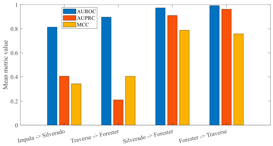
Figure 2.
Identifier-level source-target representation discrepancy across four can-train-and-test scenarios: raw identifier signatures versus within-vehicle rank-normalized behavioral-role signatures.
Figure 2.
Identifier-level source-target representation discrepancy across four can-train-and-test scenarios: raw identifier signatures versus within-vehicle rank-normalized behavioral-role signatures.
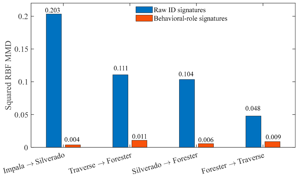
Figure 3.
Attack-family AUPRC and target-normal adaptation-budget sensitivity on can-train-and-test: (a) attack-family performance; (b) target-normal adaptation-budget sensitivity.
Figure 3.
Attack-family AUPRC and target-normal adaptation-budget sensitivity on can-train-and-test: (a) attack-family performance; (b) target-normal adaptation-budget sensitivity.
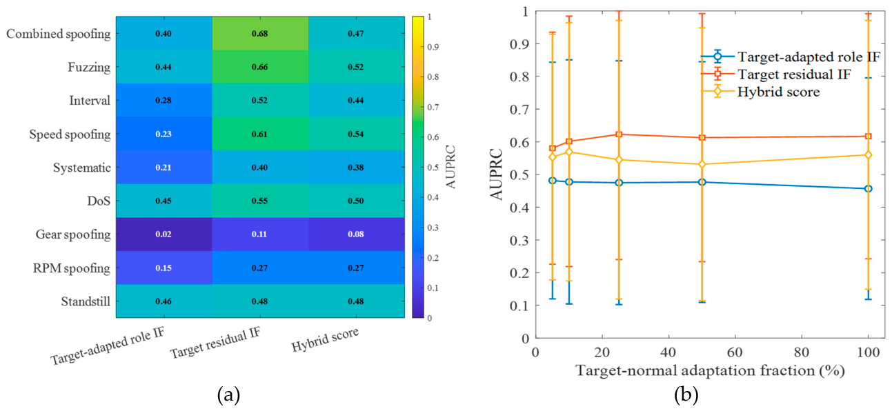
Figure 4.
Detector and fusion sensitivity analyses: (a) adapted-role detector baselines and (b) attack-label-free fusion rules.
Figure 4.
Detector and fusion sensitivity analyses: (a) adapted-role detector baselines and (b) attack-label-free fusion rules.
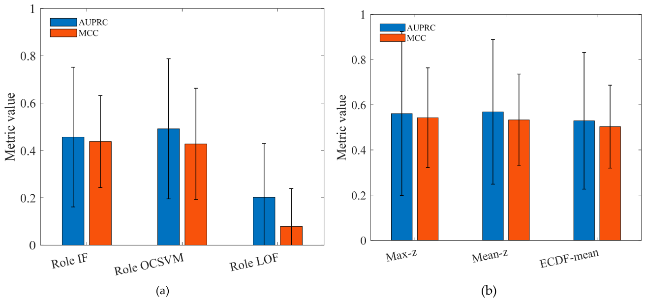
Figure 5.
Resolution-constrained, dependence-informed block lengths across four can-train-and-test scenarios. Bars show operational block length in windows; labels give the corresponding duration at 0.05 s per window.
Figure 5.
Resolution-constrained, dependence-informed block lengths across four can-train-and-test scenarios. Bars show operational block length in windows; labels give the corresponding duration at 0.05 s per window.
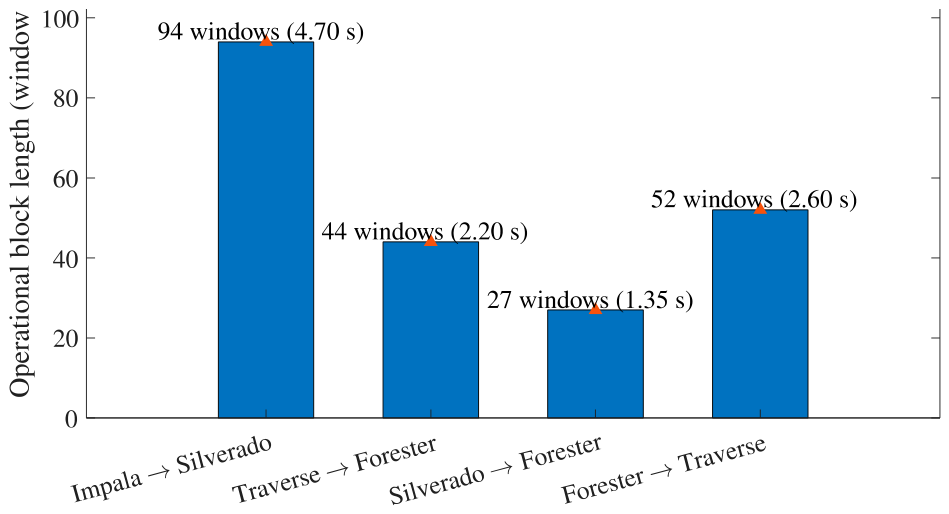
Figure 6.
Descriptive can-train-and-test block-level comparison at α = 0.05: (a) empirical block FPR; (b) attack-block recall. Window rules are mapped to blocks by an any-window alarm rule.
Figure 6.
Descriptive can-train-and-test block-level comparison at α = 0.05: (a) empirical block FPR; (b) attack-block recall. Window rules are mapped to blocks by an any-window alarm rule.
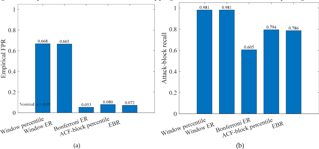
Figure 7.
Matched detector baselines and residual-feature ablations on can-train-and-test: (a) matched learning-setting and detector comparisons, reported as mean with SD across four scenarios; (b) residual feature-group ablations using Isolation Forest.
Figure 7.
Matched detector baselines and residual-feature ablations on can-train-and-test: (a) matched learning-setting and detector comparisons, reported as mean with SD across four scenarios; (b) residual feature-group ablations using Isolation Forest.
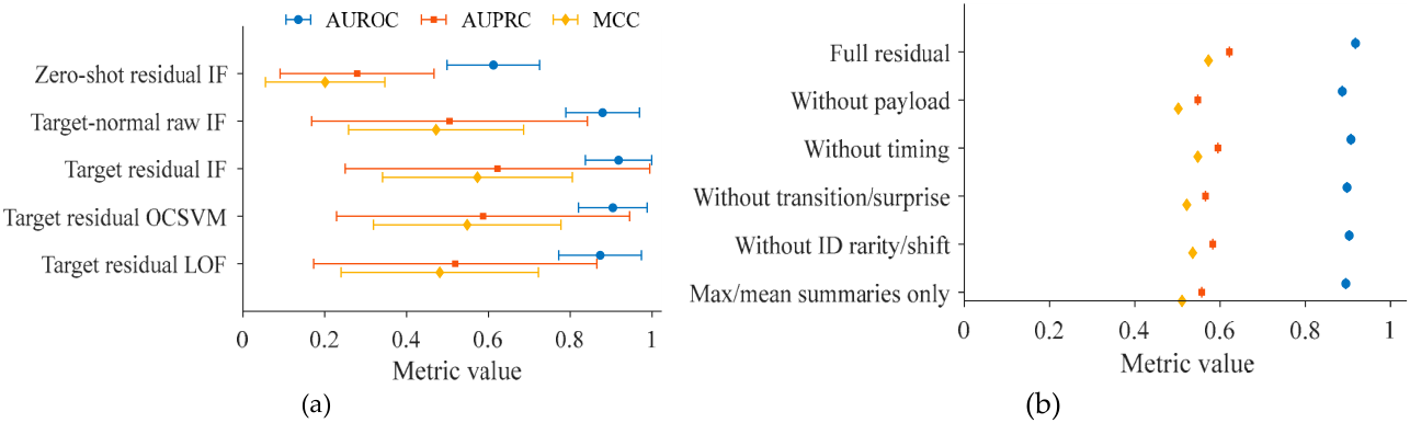
Figure 8.
Post hoc decision comparison after matching empirical evaluation-set block FPR near 0.05: (a) block FPR; (b) attack-block recall; (c) MCC; (d) median detection latency. Error bars are descriptive uncertainty intervals conditioned on the observed evaluation partitions; the matched thresholds are not deployment calibration rules.
Figure 8.
Post hoc decision comparison after matching empirical evaluation-set block FPR near 0.05: (a) block FPR; (b) attack-block recall; (c) MCC; (d) median detection latency. Error bars are descriptive uncertainty intervals conditioned on the observed evaluation partitions; the matched thresholds are not deployment calibration rules.
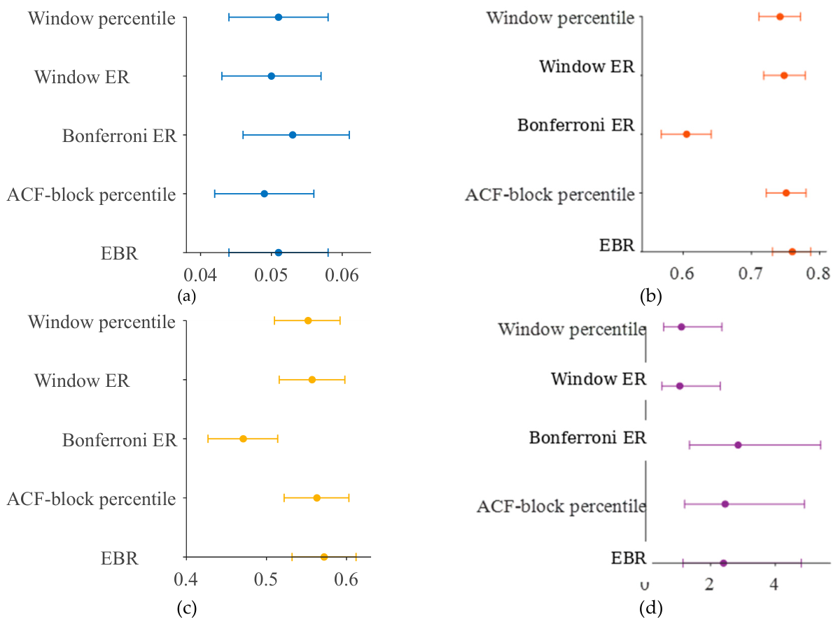
Figure 9.
Scenario-level performance of the primary target-residual IF with descriptive capture-respecting uncertainty intervals: (a) AUROC; (b) AUPRC; (c) MCC. The aggregate row summarizes the four observed scenarios and is not a population-level confidence statement.
Figure 9.
Scenario-level performance of the primary target-residual IF with descriptive capture-respecting uncertainty intervals: (a) AUROC; (b) AUPRC; (c) MCC. The aggregate row summarizes the four observed scenarios and is not a population-level confidence statement.
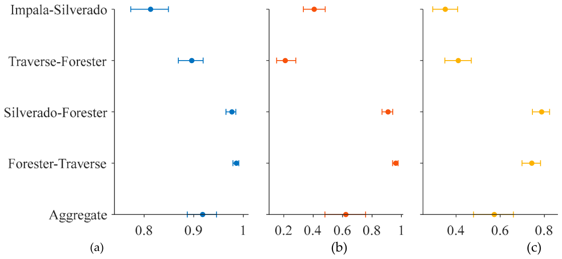
Figure 10.
Operational alarm burden for EBR at α = 0.05: (a) empirical block FPR; (b) alarm-positive blocks and merged alarm events per hour; (c) benign-state average run length; (d) median detection latency with descriptive error bars. Adjacent positive blocks were merged within 10 s and a 30 s refractory interval was applied.
Figure 10.
Operational alarm burden for EBR at α = 0.05: (a) empirical block FPR; (b) alarm-positive blocks and merged alarm events per hour; (c) benign-state average run length; (d) median detection latency with descriptive error bars. Adjacent positive blocks were merged within 10 s and a 30 s refractory interval was applied.
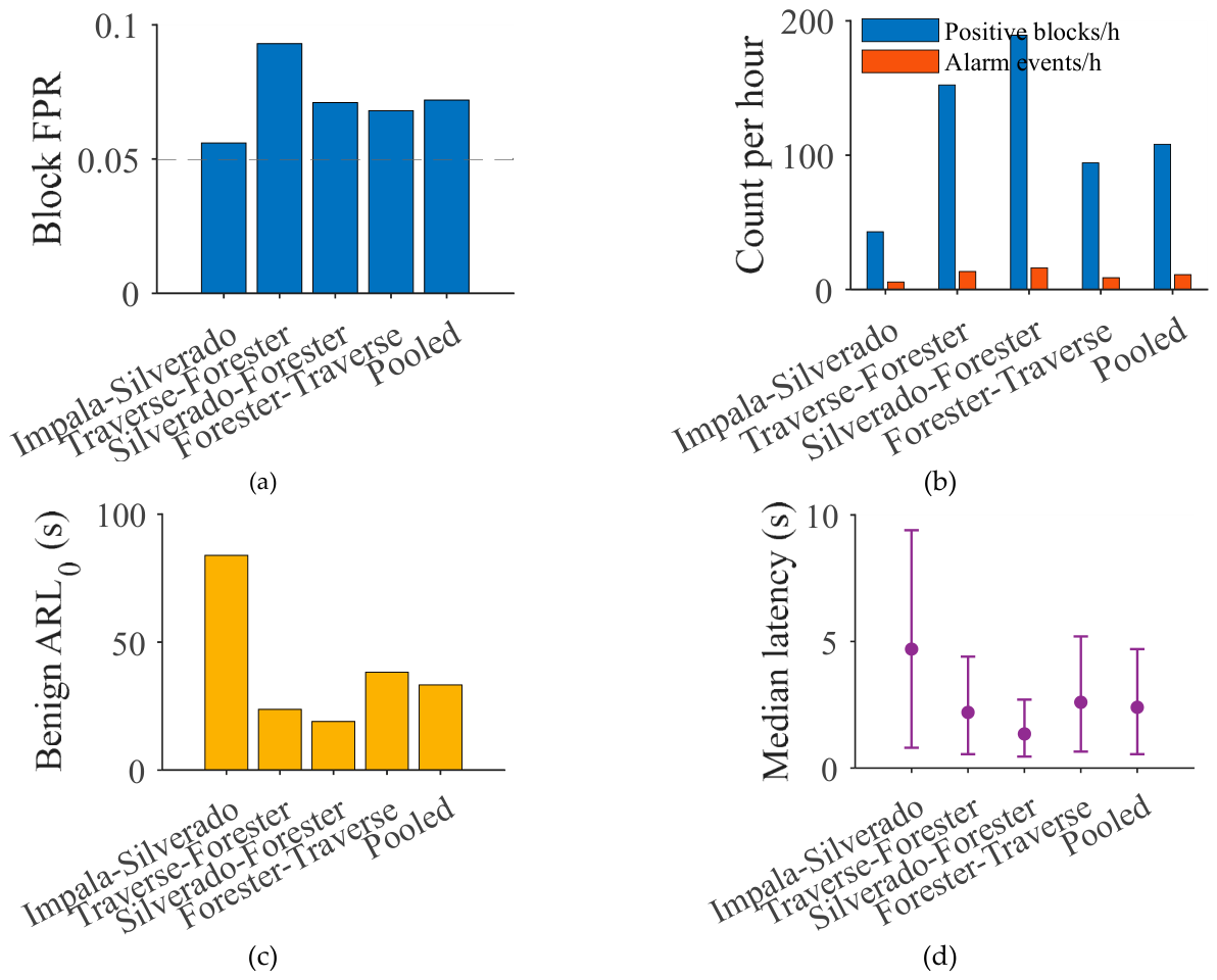
Figure 11.
Split-level stability of the ROAD target-refitted residual IF: (a) AUROC, AUPRC, and MCC; (b) attack-block recall and block FPR across five file-level splits.
Figure 11.
Split-level stability of the ROAD target-refitted residual IF: (a) AUROC, AUPRC, and MCC; (b) attack-block recall and block FPR across five file-level splits.
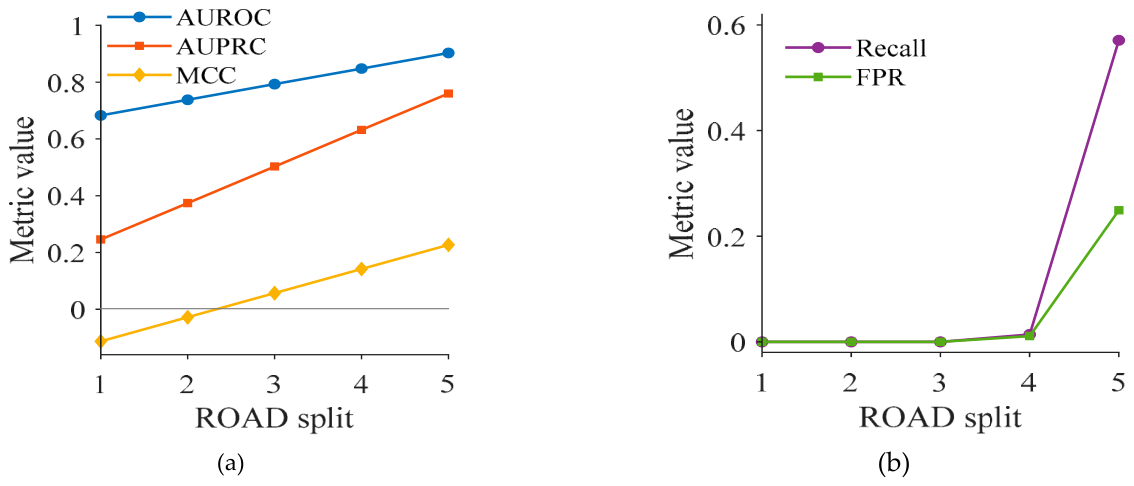
Figure 12.
Exploratory capture-level accelerator/post-exploit summary on ROAD: (a) median standardized score; (b) positive-block fraction. Green bars mark the three captures with the largest values, gray marks the intermediate Accelerator A3 capture, and blue summarizes the ambient controls; colors do not encode a validated capture-level classifier.
Figure 12.
Exploratory capture-level accelerator/post-exploit summary on ROAD: (a) median standardized score; (b) positive-block fraction. Green bars mark the three captures with the largest values, gray marks the intermediate Accelerator A3 capture, and blue summarizes the ambient controls; colors do not encode a validated capture-level classifier.
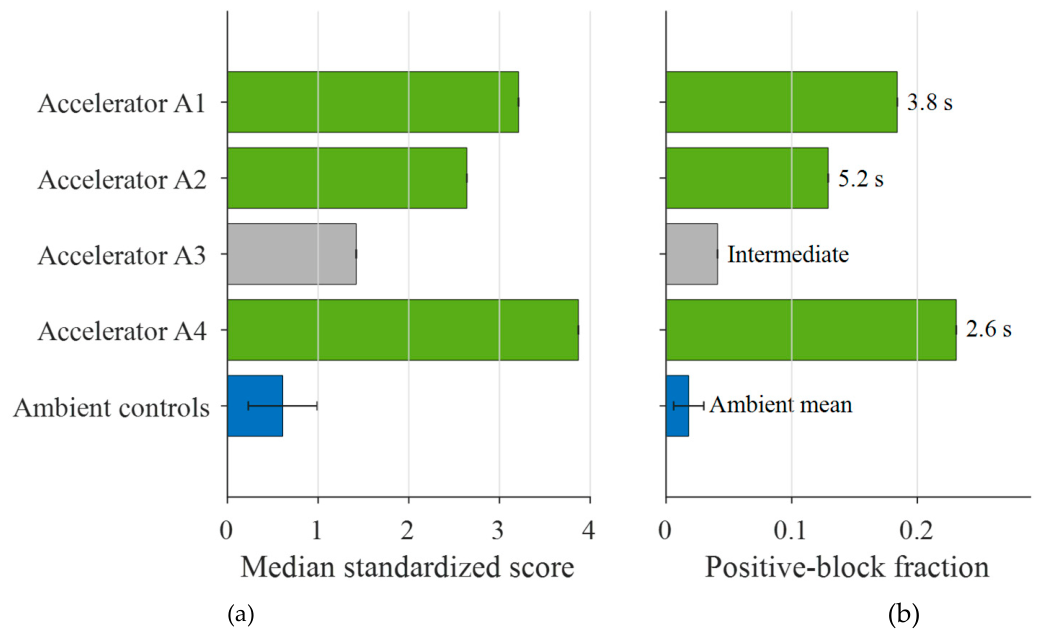
Figure 13.
ROAD cross-dataset replication: (a) target-refitted detector comparison; (b) attack-family performance.
Figure 13.
ROAD cross-dataset replication: (a) target-refitted detector comparison; (b) attack-family performance.
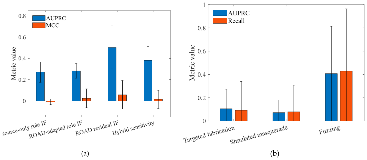
Figure 14.
ROAD calibration: (a) empirical FPR across requested α levels for Window Percentile, Window ER, Bonferroni ER, ACF-Block Percentile, and EBR; (b) benign-condition FPR shift at α = 0.05.
Figure 14.
ROAD calibration: (a) empirical FPR across requested α levels for Window Percentile, Window ER, Bonferroni ER, ACF-Block Percentile, and EBR; (b) benign-condition FPR shift at α = 0.05.
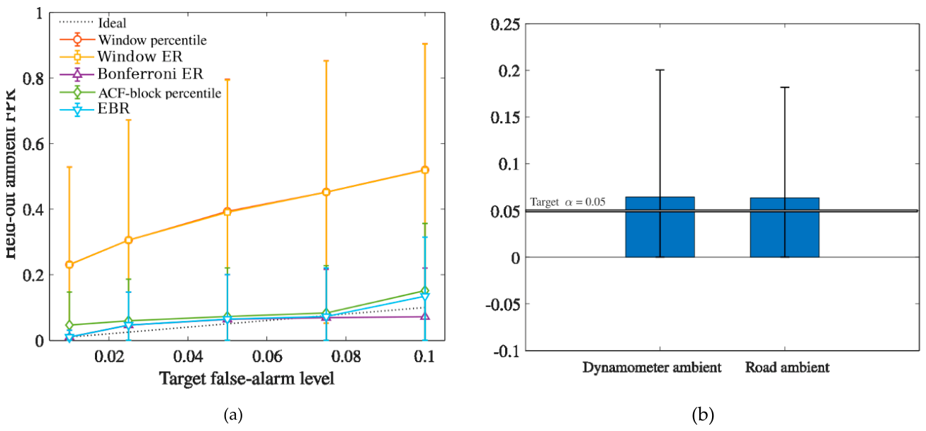
Figure 15.
Sensitivity to target-normal contamination from 0% to 10%: (a) AUROC, AUPRC, and MCC; (b) attack-block recall and block FPR.
Figure 15.
Sensitivity to target-normal contamination from 0% to 10%: (a) AUROC, AUPRC, and MCC; (b) attack-block recall and block FPR.
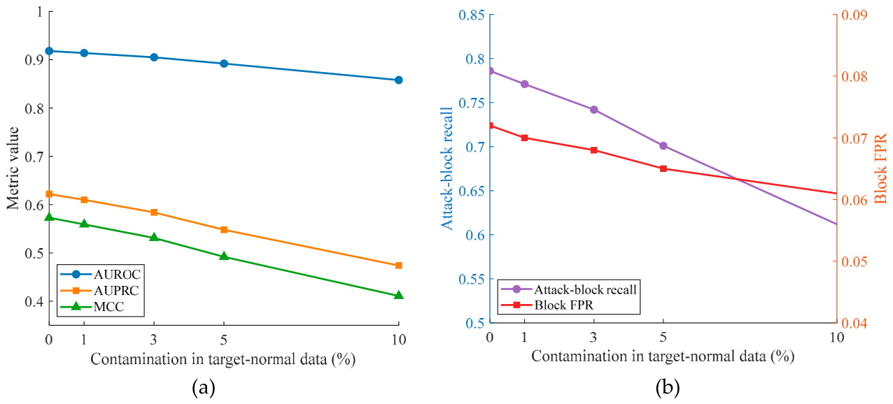
Figure 16.
EBR operating-level tradeoff: (a) block FPR; (b) attack-block recall; (c) alarm-positive blocks and merged alarm events per hour. The α grid begins at 0.01 because M = 100 provides a rank resolution of approximately 0.0099.
Figure 16.
EBR operating-level tradeoff: (a) block FPR; (b) attack-block recall; (c) alarm-positive blocks and merged alarm events per hour. The α grid begins at 0.01 because M = 100 provides a rank resolution of approximately 0.0099.
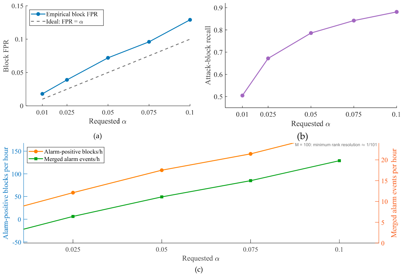
Figure 17.
Block-length sensitivity across 16, 32, 48, 64, and 96 windows: (a) block FPR and attack-block recall; (b) median detection latency.
Figure 17.
Block-length sensitivity across 16, 32, 48, 64, and 96 windows: (a) block FPR and attack-block recall; (b) median detection latency.
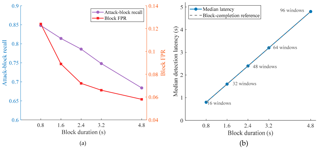

Table 1.
Prespecified analysis parameters common to the can-train-and-test and ROAD experiments.
| Setting | Parameter | Prespecified value |
| Window construction | Duration; minimum frames | 0.05 s; 8 frames |
| Residual scoring | Magnitude clip; unseen-event penalty | 12; 8 |
| Rare-identifier rule | Positive-probability cutoff | Bottom 20% |
| Isolation Forest | Trees; maximum observations per learner | 100; 256 |
| Behavioral baseline | Source-to-target window ratio | 1:4 |
| ACF search | Initial lags; extension; maximum; in-band run | 80; 40; 240; 8 lags |
| Rank resolution | Minimum calibration blocks | 100 |
| Alarm levels | Evaluated α; default α | {0.01, 0.025, 0.05, 0.075, 0.10}; 0.05 |
| Target-normal split | Oracle-clean prefix reserved; adaptation/calibration | 40%; equal chronological halves |
| Repeated fits | Isolation Forest seeds per scenario | 5 |
| Event post-processing | Merge horizon; refractory interval | 10 s; 30 s |
Table 2.
Target-adaptive anomaly-scoring performance and descriptive block-level decisions on can-train-and-test. Anomaly-scoring metrics are mean (SD) across four vehicle scenarios; decision metrics are evaluated at α = 0.05.
Table 2.
Target-adaptive anomaly-scoring performance and descriptive block-level decisions on can-train-and-test. Anomaly-scoring metrics are mean (SD) across four vehicle scenarios; decision metrics are evaluated at α = 0.05.
| Representation and anomaly-scoring performance | ||||
| Method | AUROC | AUPRC | AUPRC lift | MCC |
| Raw source IF | 0.567 (0.140) | 0.248 (0.239) | 2.928 (2.047) | 0.158 (0.218) |
| Behavioral-role source IF | 0.498 (0.120) | 0.161 (0.131) | 1.773 (0.479) | 0.109 (0.077) |
| Target-adapted role IF | 0.854 (0.056) | 0.456 (0.331) | 5.292 (2.112) | 0.438 (0.212) |
| Target-adapted role OCSVM | 0.857 (0.063) | 0.492 (0.330) | 6.214 (3.097) | 0.427 (0.253) |
| Target-adapted role LOF | 0.585 (0.105) | 0.202 (0.255) | 1.761 (0.689) | 0.079 (0.180) |
| Target residual IF (primary) | 0.918 (0.081) | 0.622 (0.372) | 7.805 (2.962) | 0.573 (0.232) |
| Hybrid role+residual sensitivity | 0.915 (0.087) | 0.561 (0.407) | 6.446 (2.471) | 0.543 (0.246) |
| Descriptive block-level decision comparison at the default operating point | ||||
| Decision rule | Block FPR at α = 0.05 | Attack-block recall | Interpretation | |
| Window Percentile | 0.668 | 0.981 | Window threshold mapped to any-window block alarm | |
| Window ER | 0.665 | 0.981 | Window empirical rank mapped to any-window block alarm | |
| Bonferroni ER | 0.053 | 0.605 | Within-block multiplicity correction | |
| ACF-Block Percentile | 0.080 | 0.794 | Empirical threshold for block maxima | |
| EBR | 0.072 | 0.786 | Empirical ranking of block maxima; descriptive under unresolved dependence | |
Table 3.
ROAD cross-dataset replication after target-specific refitting. Values are mean (SD) across five overlapping file-level splits.
Table 3.
ROAD cross-dataset replication after target-specific refitting. Values are mean (SD) across five overlapping file-level splits.
| Method | AUROC | AUPRC | AUPRC lift | MCC | Attack-block recall | Block FPR |
| Source-only behavioral-role IF | 0.519 (0.093) | 0.270 (0.095) | 1.035 (0.158) | −0.009 (0.026) | 0.026 (0.059) | 0.028 (0.054) |
| ROAD target-adapted behavioral IF | 0.522 (0.085) | 0.282 (0.068) | 1.111 (0.222) | 0.024 (0.088) | 0.040 (0.088) | 0.017 (0.031) |
| ROAD target-refitted residual IF (primary) | 0.793 (0.087) | 0.503 (0.203) | 1.905 (0.391) | 0.057 (0.134) | 0.117 (0.254) | 0.052 (0.110) |
| Hybrid role+residual sensitivity | 0.666 (0.073) | 0.381 (0.129) | 1.469 (0.276) | 0.015 (0.086) | 0.051 (0.113) | 0.027 (0.051) |
Table 4.
Capture-separation, normal-only baseline, and 5% target-normal contamination results. Values are scenario-aggregated point estimates.
Table 4.
Capture-separation, normal-only baseline, and 5% target-normal contamination results. Values are scenario-aggregated point estimates.
| Configuration or method | AUROC | AUPRC | MCC | Attack-block recall | Block FPR |
| Capture-partition sensitivity analysis | |||||
| Same-capture chronological | 0.918 | 0.622 | 0.573 | 0.786 | 0.072 |
| Capture-disjoint | 0.889 | 0.553 | 0.486 | 0.714 | 0.079 |
| Leave-one-capture-out | 0.875 | 0.521 | 0.451 | 0.681 | 0.083 |
| Stronger normal-only baselines | |||||
| Target-normal raw IF | 0.879 | 0.505 | 0.472 | 0.682 | 0.077 |
| MLP-AE | 0.892 | 0.546 | 0.492 | 0.701 | 0.080 |
| LSTM-AE | 0.903 | 0.578 | 0.526 | 0.728 | 0.078 |
| Deep SVDD | 0.910 | 0.600 | 0.555 | 0.749 | 0.075 |
| TCN-AE | 0.914 | 0.609 | 0.562 | 0.762 | 0.074 |
| Residual IF | 0.918 | 0.622 | 0.573 | 0.786 | 0.072 |
| Diagnostic at 5% target-normal contamination | |||||
| Adaptation only | 0.894 | 0.556 | 0.501 | 0.719 | 0.074 |
| Calibration only | 0.913 | 0.601 | 0.538 | 0.676 | 0.057 |
| Adaptation and calibration | 0.892 | 0.548 | 0.492 | 0.701 | 0.065 |
Disclaimer/Publisher’s Note: The statements, opinions and data contained in all publications are solely those of the individual author(s) and contributor(s) and not of MDPI and/or the editor(s). MDPI and/or the editor(s) disclaim responsibility for any injury to people or property resulting from any ideas, methods, instructions or products referred to in the content. |
© 2026 by the authors. Licensee MDPI, Basel, Switzerland. This article is an open access article distributed under the terms and conditions of the Creative Commons Attribution (CC BY) license (http://creativecommons.org/licenses/by/4.0/).
Copyright: This open access article is published under a Creative Commons CC BY 4.0 license, which permit the free download, distribution, and reuse, provided that the author and preprint are cited in any reuse.