

Submitted:
17 September 2026
Posted:
18 September 2026
You are already at the latest version
Abstract
A clay flow rule governs contraction or dilation during plastic shearing. A fractional replacement must preserve the zero-dilatancy critical state and remain compatible with elasticity and hardening. We examine these requirements for a terminal-directed Caputo operator on a teardrop surface. The operator integrates surface slopes over a logarithmic stress interval, not elapsed loading history. Analytical derivations and incremental tests separate terminal compatibility, operator composition, stress-path identifiability and admissibility. The operator zero matches the non-associated base-model critical state only if Ω = Ψ. For kaolin, the alternative zero raises the normally consolidated undrained terminal mean stress by 18.6%. An exact identity shows why the flow candidates share the same normally consolidated stress locus yet progress differently in a numerical coordinate. Mean-stress preservation permits exact scalar composition with the SMP transformation but supplies no physical strain mapping. Two direct overconsolidated substitutions expose distinct deficiencies: coupling the loading modulus to the fractional dilatancy (F2) reverses its sign above OCR=exp(1/Ψ), whereas retaining the inherited loading modulus (F1) causes hardening inconsistency, low-OCR surface drift or negative assigned work at high OCR. These results define requirements a fractional clay formulation must satisfy before stress and strain data can test its predictions.
Keywords:
fractional plasticity
; transformed stress
; caputo derivative
; critical state
; constitutive admissibility
; clay
1. Introduction
When saturated clay is sheared, its skeleton can tend to contract or dilate. A constitutive flow rule describes the irreversible volumetric deformation accompanying plastic shear. Under the ideal undrained constraint used here, total volumetric deformation is zero: the plastic tendency must be balanced by an elastic volumetric increment, which changes mean effective stress. The flow rule therefore matters even when the specimen cannot change its total volume. Critical-state clay plasticity connects this response to the loading surface, elastic compressibility and hardening [1,2]. The present question is whether replacing one flow ingredient by a fractional operator preserves those connections.
The fractional ingredient considered here is a weighted integral of slopes along a prescribed stress-space meridian. Its intended constitutive role is to supply a scalar contraction–dilation ratio. This is a phenomenological choice at continuum scale: neither a grain-scale derivation of the kernel nor a time-memory law is supplied. Stress-fractional approaches have used related ideas to construct non-associated response without an independently prescribed plastic potential [3,4,5,6,7]. Our component-interaction study combined a teardrop surface, a fixed-window fractional flow approximation and nonlinear compression [8]. The subsequent closed-form study established the teardrop terminal and evaluated a terminal-directed Caputo operator, while distinguishing the surface apex from the embedded non-associated critical state [9]. Here we examine what follows when that established scalar construction is coupled to specified incremental equations.
The first physical question is where plastic volume change ceases during continued shearing. In the published non-associated base model, the radial-mapping flow rule vanishes at the transformed stress ratio [10]. A terminal chosen from the stationary point of the teardrop surface instead places the zero according to the surface-shape parameter . The two states need not coincide when the second surface parameter is independent. Calling either point a critical state does not establish that the same limiting stress and volume response has been retained. We derive the condition for coincidence and calculate the resulting difference in an undrained terminal stress.
A second question arises in three dimensions. Soil strength depends on the relative principal stresses, so a meridional pressure–deviator relation must be connected to compression, extension and other Lode angles. The Spatially Mobilised Plane (SMP) transformation provides such a stress representation by preserving mean stress and changing the deviatoric radius [11,12,13]. A nonlocal operator samples an interval, whereas an ordinary Jacobian describes a local change. The usual local chain rule therefore cannot be assumed for a fractional stress derivative [4,14]. We identify a sufficient condition under which the present scalar integral is unchanged by the transformation, and keep that statement separate from the strain mapping required for a complete physical model.
The third question is how the selected flow changes the incremental response. We first eliminate volumetric deformation and hardening to derive the normally consolidated undrained stress locus. This shows why a close stress-path fit may carry no independent information about the flow direction. We then test two direct substitutions in the inherited overconsolidated loading structure: retaining its loading modulus, or coupling that modulus directly to the fractional dilatancy. The purpose is to expose the consequences of these precise choices before calibration. The contributions beyond [9] are the explicit terminal-compatibility condition, the exact normally consolidated locus identity, the invariant-coordinate composition criterion and the incremental substitution diagnostics. Together they specify requirements for subsequent model development; they do not constitute a validated three-dimensional fractional clay model.
1.1. Relation to Existing Models and Organization of the Study
Fractional soil models use different mathematical objects. A component-wise fractional gradient requires a multiaxial definition [5,6,7], while state-dependent scalar stress–dilatancy relations specify one part of the flow [5,6,15]. Recent formulations include shift stress, cyclic interfaces, overconsolidation, reduced elastic domains and dissipation analysis [16,17,18,19,20]; anisotropic clay models additionally introduce rotational hardening [7,21]. Bounding-surface response, non-coaxiality and calibration are separate parts of the constitutive architecture [22,23,24]. Our one-dimensional meridional integral provides none of those components by itself. Table 1 identifies the question answered by each part of this study and the evidence needed to connect it to physical prediction.
Section 2 introduces the physical assumptions, stress variables and numerical update. Section 3 asks whether the prescribed zero represents the same terminal state as the base model. Section 4 treats the stress transformation. Section 5 examines the common normally consolidated locus and the two overconsolidated substitutions. Section 6 interprets what the calculations establish about model construction and what remains to be tested experimentally.
Table 1 is the logical map of the study. Coordinate composition asks whether the same scalar operation is obtained before and after changing the stress representation. Terminal compatibility asks whether the zero selected by that operation is the state at which the inherited material model permits continuing shear without further plastic volume change. Incremental consistency asks whether the stress increment, plastic volume change and evolution of the surface size satisfy one common set of equations. The work-sign test then asks a separate question about the declared stress–plastic-coordinate pairing, whereas experimental validation requires measured observables that are actually sensitive to the chosen flow. Passing one test therefore supplies no automatic evidence for the next. This separation is used throughout the paper to prevent a mathematical property of one scalar quantity from being read as validation of a complete constitutive model.
2. Physical Basis and Mathematical Construction
2.1. Physical Assumptions and the Role of Each Equation
We work at the scale of a homogeneous material point, using an effective-stress, small-increment elastoplastic description. Elastic volumetric deformation is recoverable; plastic volumetric deformation changes the hardening state. For the ideal undrained calculations, their increments sum to zero. This provides a simple physical reading of the pressure update: with compression positive and bulk modulus , a contractive plastic increment requires elastic expansion and hence . A dilative plastic increment has the opposite effect. These implications follow from the stipulated volume balance. No pore-pressure field or drainage problem is solved.
The surface describes the stress states associated with the current hardening scale. The flow rule selects the relative plastic volumetric and shear increments. The plastic multiplier sets their magnitude, and hardening describes how the surface changes after plastic volume change. These ingredients must agree: using one volume increment to change stress and a different one implicitly to change the surface breaks the intended consistency relation. The overconsolidated tests below examine precisely that issue.
In a physical meridional model, dilatancy would be a ratio of plastic volumetric to plastic shear strain increments. Here we first define the analogous scalar-coordinate ratio during active plastic loading. Positive means contraction and negative means dilation within this declared coordinate system. The variable is introduced through a transformed elastic update and has not been proved equal to measured shear strain. A zero of is therefore called an operator zero or candidate terminal until the remaining stress, hardening and kinematic conditions are specified.
2.2. Teardrop Surface and the Two Candidate Terminals
Compression is positive. Mean effective stress measures the isotropic part of stress carried by the soil skeleton. A tilde distinguishes the transformed deviatoric magnitude from the real magnitude ; all extension deviators are reported as non-negative magnitudes. Define . The current surface size has stress units and changes with plastic volumetric deformation. The positive dimensionless parameters , and specify the transformed critical stress ratio and the teardrop geometry. The inherited loading surface [10] is
At isotropic loading, Equation (1) gives the intercept . Thus records the pressure scale of the current surface, rather than a fixed normalization. With , and , its positive meridian becomes
The coordinate increases as pressure decreases relative to the current surface size. It is dimensionless and is not time. In Equation (2), controls the exponent and hence the curvature; also scales the stress ratio at a given . These are phenomenological surface parameters, not separately measured microstructural quantities. Along the surface, the base-model condition gives . Differentiating the surface ordinate instead gives a stationary point at . Subscripts and distinguish the material terminal selected by the base flow from the surface stationary point.
The same coordinate needs a different reading at an overconsolidated initial state. Under the normalization used in the scalar diagnostics, the isotropic starting value is ; this is a geometric statement about the position of the current stress relative to the outer-surface size. It is not a record of how long the specimen has been loaded. Likewise, the prescribed value is the destination of the terminal-directed integration interval, not a reversal point in a chronological loading path. A cyclic-memory interpretation would require additional history variables and update rules that are absent here. To keep the two endpoint descriptions visible, the labels ‘op’ and ‘*’ both denote the operator-defined terminal, whereas ‘base’ and ‘b’ denote the independently selected base-model terminal.
2.3. What the Terminal-Directed Caputo Operator Represents
An ordinary associated flow rule uses the local normal to a surface. The present construction replaces one local slope by an integral of meridional slopes between the current stress coordinate and a prescribed terminal. For and , we define the candidate by
The kernel weights slopes closer to the evaluation point more strongly, with controlling that weighting. The chosen orientation gives a positive value on the side and a negative value on the side. The interval collapses at , where the value is prescribed as zero. These are construction properties. Interpreting the output as a volumetric-to-shear plastic-coordinate ratio is the additional constitutive assumption tested below. During each evaluation, , , and are held fixed. The sampled points belong to the current meridian; they need not be states previously visited by the specimen. In particular, Equation (3) contains no elapsed time, loading rate or stored reversal history.
Standard fractional definitions are given in [25,26], and the earlier closed-form construction is reported in [9]. Under its notation, the present sign convention is ; the earlier pressure-coordinate evolution contains the additional positive factor , and recovering physical dilatancy introduces . Those factors preserve the zero and sign of the present integral but change its magnitude. We deliberately test Equation (3) directly as , so our trajectories must not be read as reproductions of that earlier evolution law.
As , Equation (3) tends to at an interior point. The associated pressure-coordinate slope would instead involve . Thus the integer-order limit of this integral is well defined, but does not by itself recover the complete associated constitutive model. The reference value is inherited, not calibrated against the present records. At , the integral is finite only if ; all sign proofs use , and the numerical cutoff is specified in Section 2.5.
This distinction also clarifies the limited meaning of nonlocality in the present paper. The ordinary surface normal uses the slope at the current stress coordinate, whereas Equation (3) combines slopes from the current coordinate to the prescribed terminal on the same current meridian. The parameter changes the relative geometric weight assigned within that interval. Because the interval is in stress space, is not interpreted here as viscosity, a rate parameter or a measure of temporal memory. Its physical identification would require observations and a complete stress–strain relation that are not part of this audit.
2.4. Why Transformed Stress Is Introduced
For positive principal effective stresses , let , and , and define = − and = − 9. Write and , where is the identity tensor. The operational SMP-equivalent deviator used in the supplied implementation, away from the hydrostatic state, is [11,12]
Equation (4) changes the deviatoric radius while preserving mean effective stress. Under triaxial compression the implemented radius equals the real deviator; under extension the inverse is . This allows a common transformed stress ratio to correspond to different real compression and extension strengths. At the hydrostatic state, both deviators vanish and the mapped stress is taken as . The scalar composition proof uses only the invariance of and, for fixed , of . It does not require or establish differentiability of the complete tensor mapping at every hydrostatic approach.
2.5. Data Provenance and Numerical Protocol
The numerical sets in Table 2 were carried forward from the base-model calibration files associated with [10]; no parameter is fitted in the present study. The Fujinomori stress points used here were digitized from Matsuoka et al. [12], which attributes the original test to Nakai and Matsuoka [27]. The kaolin parameter lineage is the Banerjee--Stipho test family [28,29], using plots reproduced by Xu et al. [30]. Eastern Osaka is represented only by an inherited parameter set associated with the natural-clay study [31], not by a validated trajectory here. S1 identifies the files actually used and preserves additional transcriptions without treating them as evidence for the fractional candidate. In particular, the kaolin pair is distinct from the Wroth--Loudon pair used in [8].
We evaluate Equation (3) by SciPy algebraically weighted quadrature [32]. A table with 1800 distance-coordinate points on each side of the terminal includes the exact zero and 500 extra geometric points near the isotropic cutoff. Comparison with direct quadrature at 30 seeded interior pressures and 70 pressures between 0.985 and 0.9995 gives a maximum absolute discrepancy of . The evaluation is capped at , and the table spans . This cutoff defines the numerical initial neighborhood; it is not an independently measured material parameter.
The imposed variable enters the scalar elastic update . We use , and . Fujinomori runs use 240,000 increments to ; kaolin F1 diagnostics use 60,000 increments to . Initial conditions are , , and . Appendix B gives the multiplier, image-point evaluation, explicit update and stopping rules so that the link between flow and output is fully specified.
The incremental cause-and-effect sequence is therefore as follows. An imposed supplies a transformed shear-loading increment. Together with the elastic moduli, surface-normal components, loading modulus and selected flow ratio , it determines the plastic multiplier .
The resulting multiplier sets the plastic shear and volumetric-coordinate increments. The volumetric increment changes through hardening, while the zero-total-volume condition produces the accompanying change in ; the transformed deviator is then updated and the next values of and are evaluated from the new state. A change in consequently propagates through pressure, hardening and the next surface location. This is why replacing the flow factor without rederiving the multiplier and hardening terms is not a local cosmetic substitution.
To compare with the experiment, calculated stresses are converted back to real triaxial extension coordinates. Measured strain is not overlaid on : the differential of the nonlinear stress map, discussed in Section 4.3, has not been coupled here to a physical strain transformation. Two additional diagnostics are the surface residual and a declared plastic-work increment
The tests impose . In Equation (5), is on the surface and is outside it. The second expression is the work assigned to the declared transformed stress–plastic-coordinate pairing, evaluated at the pre-increment stress. We monitor its sign, the loading-modulus sign and the algorithmic denominator separately. A negative value fails the chosen work condition; calling that quantity physical dissipation would additionally require a strain mapping and a stored-energy model. S1 documents the reproduction environment: Python 3.12.14, NumPy 2.3.5, SciPy 1.17.0 and Matplotlib 3.10.8.
3. Does the Operator Preserve the Intended Critical State?
3.1. Exact Condition
At a critical state, continued shearing should be possible without continuing change in stress or volume within the adopted idealization. A zero of volumetric flow is therefore necessary, but by itself is not a complete critical-state condition. We first locate the zero imposed by the scalar construction. Differentiating Equation (2) gives
The derivative changes sign at , which is the zero anchoring Equation (3). On the positive meridian, its stress coordinates are
In the base radial-mapping model, the normally consolidated rule is . Continued plastic shear therefore has zero volumetric increment at , which gives . Comparing that independently selected state with Equation (7) yields
The two definitions select the same point if and only if , independently of fractional order. The physical issue is that the zero specifies where the chosen contraction–dilation mechanism ceases. Moving it changes the candidate terminal stress, even though the yield-surface equation itself has not been changed. Because the base model is non-associated, its zero need not lie at the surface apex. Equality of the terminals also does not imply equality of the complete flow direction or of its magnitude away from that point.
3.2. Consequence for Normally Consolidated Undrained Terminals
The consequence for an undrained specimen follows from the declared volume balance. Elastic compression contributes , while isotropic hardening gives . Setting their sum to zero links a change in surface size to a change in effective pressure. For , integration from the isotropic normally consolidated pressure to either candidate zero gives
Equation (9) evaluates the two candidate endpoints on the normally consolidated locus; reaching them requires an admissible incremental branch. The calculation depends on the ratio of the two compression coefficients, so a common specific-volume normalization cancels. The complete derivation of the locus is given in Section 5.1. Table 3 distinguishes the surface coordinate from the terminal mean stress normalized by the initial pressure .
For the compatible Fujinomori pair, both constructions select the same terminal. For Eastern Osaka, their normally consolidated mean stresses differ by about 1.6%. The kaolin separation is larger: the operator zero is at , and its candidate terminal pressure is 18.6% above that selected by the base flow. Thus a change presented as only a replacement of the flow can also change the limiting undrained effective-stress state. The 18.6% is a difference between two model-defined endpoints under identical inherited coefficients; it is not a measured prediction error. Figure 1 illustrates the geometry behind this difference.
This pressure difference has a conditional undrained interpretation: if two material-point calculations share the same prescribed total mean stress, the relation would assign the higher effective pressure to a lower pore pressure by the same amount. No total-stress path or pore-pressure prediction is supplied here, so Table 3 reports effective-stress endpoints only. The comparison demonstrates why the location of a volumetric-flow zero matters physically without claiming a new pore-pressure validation.
4. Can the Scalar Operator Be Carried Through a Stress Transformation?
4.1. Why the Ordinary Local-Chain Substitute Fails
A nonlinear coordinate map changes distances throughout the interval sampled by a fractional operator. Its Jacobian at the current state therefore need not reproduce the transformed weighting of all the sampled slopes. To show this directly, let be smooth and strictly increasing, let , and let be continuously differentiable on the transformed interval. For a left-sided Caputo derivative with terminal , differentiating the composite inside the integral gives
The common local-chain substitute multiplies a derivative evaluated in the transformed coordinate by the current Jacobian,
The exact expression contains the local derivative at every integration point and the kernel measured in the original coordinate. The substitute evaluates a different integral in the transformed coordinate and multiplies it by only at the endpoint. For the illustrative map , , and , independent weighted quadrature gives a relative discrepancy of 19.704% at (Figure 2). The map coefficient and parameter values are illustrative choices, not values fitted to any clay; the marked fractional order is the inherited reference value stated in Section 2.3. This is a counterexample to the proposed local-chain substitute, not a 19.704% error of the SMP mapping or of a clay prediction. The discrepancy tends to zero as approaches one, when the ordinary derivative is recovered.
4.2. A Sufficient Invariant-Coordinate Criterion
The failure of Equation (11) does not prevent every transformed-stress use. A narrower construction avoids a chain rule altogether. Let a scalar state function be , where is absolutely continuous on the integration interval. Let be a one-dimensional nonlocal operator acting only in , with all other state variables held fixed, and let the stress transformation satisfy . If the integration terminal is expressed in the same invariant coordinate, then
Both sides integrate the same function over the same interval with the same kernel, because the transformation leaves the integration coordinate and terminal unchanged. This proves a sufficient criterion for the scalar construction. It is not a general chain rule for component-wise fractional gradients. In physical terms, the stress representation may change the deviatoric radius while leaving the pressure coordinate sampled by this particular operator untouched.
4.3. SMP Corollary and Its Boundary
For Equation (3), the integration coordinate is . Equation (4) preserves , and is held fixed as an internal scalar during the integral evaluation. Consequently, both and remain unchanged: applying the stress transformation before or after the scalar operation gives the same value. This establishes coordinate compatibility for the chosen meridional integral.
A corresponding physical strain transformation is a separate requirement. For example, differentiating the extension inverse gives . Both stress increments contribute. It is therefore not justified to reinterpret the coordinate in as measured shear strain solely because the scalar integral is invariant. The real-stress elasticity and transformation derivatives in [12] illustrate why this extra step matters. In this study, remains a declared numerical coordinate.
The distinction can also be expressed through power. A stress transformation becomes constitutively complete only after a dual strain transformation is chosen so that the stress–strain power is preserved. Mean-stress invariance and equality of the scalar Caputo integral establish neither that dual relation nor work conjugacy. The exact scalar composition proved here is therefore a statement about representation of the stress-coordinate operation; it is not, by itself, a proof that is a physical shear-strain increment or that the transformed stress product equals material dissipation.
5. What the Incremental Calculations Establish
5.1. Normally Consolidated Fujinomori Stress Locus and Loading Coordinate
The Fujinomori pair satisfies , so terminal mismatch does not obscure the comparison. We keep the same surface, elastic coefficients, hardening, stress transformation and initial state. One run uses the inherited radial-mapping dilatancy; the other uses Equation (3) with the loading modulus coupled consistently at normal consolidation. The calculation isolates the consequences of that scalar substitution. Neither run is presented as a complete reproduction of all ingredients in a published three-dimensional model.
The effective-stress locus can be determined without solving for either plastic multiplier. Under zero total volume change, elastic volume change and plastic hardening cancel. Since , their differential relation becomes
This equation says that pressure loss and growth of the surface size are linked by the prescribed compression coefficients. Substitution into the surface relation and integration from give
No flow ratio appears in Equation (14). Under these assumptions, changing the flow ratio changes the progression along an admissible reachable branch, while the equations fixing that branch in stress space remain the same. Accordingly, Table 4 gives nearly identical effective-stress-path RMS discrepancies, 4.31200% and 4.31311% of . The difference of about 0.0011 percentage point reflects numerical integration and curve sampling along their common locus. The shared agreement in Figure 3a therefore tests the adopted stress locus; it cannot identify the fractional order or validate one flow candidate over the other.
The progression coordinate does change. The first crossing of 99% of the analytical terminal occurs at for the base candidate and 2.99 for Equation (3), as shown in Figure 3b. Appendix A explains this through two contributions: the elastic shear increment and the plastic shear coordinate required to balance volumetric hardening. The target is the analytical terminal, not the deviator reached at the imposed 15% endpoint. Independent path integration gives 1.44549% and 2.98886%; the 240,000-step values differ by less than 0.0015 percentage point and converge toward them under refinement.
For transparency, the ESP metric is the root-mean-square difference in real at the digitized experimental values of , multiplied by 100. The computed curve is interpolated in pressure; this is not an orthogonal distance or a strain-matched residual. The common calculated locus can consequently agree with the same stress points while the two internal parameterizations differ. A physical flow comparison would need an independently defined strain mapping and strain-sensitive observations.
Figure 3 should be read in two stages. Panel (a) shows that the adopted surface, volume balance and hardening constrain both calculations to essentially the same curve in effective-stress space. Panel (b) then shows that the two calculations use different amounts of the internal coordinate to traverse that curve. These observations are complementary rather than contradictory: the first concerns the locus, and the second concerns its numerical parameterization. In particular, the approximately twofold difference between the marked values must not be translated into a twofold physical strain, time or stiffness without the missing kinematic and work-conjugate mapping.
5.2. Why Direct Overconsolidated Substitutions Need Further Equations
An overconsolidated initial state lies inside the current outer surface. The inherited bounding-surface architecture therefore introduces an image point on that surface and a radial mapping ratio . In the supplied implementation, and . The ratios and enter different equations: controls plastic volume change, while controls the loading modulus. The inherited exponent is . This separation is important because an interior state can require a different loading stiffness even when the flow changes sign.
We examine two explicit choices. F1 replaces by Equation (3) in the plastic increments but retains the inherited loading modulus. F2 also replaces the dilatancy-dependent factor in that modulus. With and the positive common flow scale , they are
The candidate in these tests is evaluated at the actual normalized pressure , with the stated cutoff. The surface normal and common scale are evaluated at the image point. This choice is part of the experiment on equations, not a general fractional bounding-surface prescription. F1 and F2 are neither new validated models nor implementations of the complete architectures in [7,17]. Their purpose is to determine which inherited relations survive each direct substitution.
5.2.1. Analytical Sign Boundary for F2
Equation (6) is positive on one side of and negative on the other. Since the kernel in Equation (3) is positive, the integral has the same respective signs for every and . At the isotropic overconsolidated initial state, and . All other factors in are positive, hence
For , the boundary is . In F2, a candidate dilative response at a larger OCR is therefore tied directly to a negative loading modulus. Dilative plastic volume change is not itself the failure: the failure is the loss of the positive-modulus loading structure that this substitution is intended to retain. Figure 4a shows that changing changes the magnitude but cannot move the boundary. The numerical illustration spans ; the exactly isotropic NC evaluation uses the stated cutoff.
5.2.2. Transformed Plastic Work and Consistency Conditions for F1
For the declared transformed-stress pairing, the plastic coordinate increments are and . During active plastic loading with , and , Equation (5) reduces to
For positive , and active plastic multiplier, the bracket is the entire sign condition for the declared work pairing. A negative candidate makes the volumetric contribution negative; sufficient positive shear work can compensate only when . Figure 4b shows that balance. When the plastic multiplier is zero, the assigned plastic work is zero irrespective of the bracket. This interpretation explains the computed sign without equating it to a general thermodynamic dissipation theorem.
The other F1 defect concerns the connection between volume change and hardening. At normal consolidation, consistency requires the stress increment and the surface-size increment to satisfy the differential of Equation (1). Because changes through the adopted plastic volumetric increment, its contribution to the loading modulus must use the same as the flow. Retaining the base factor after changing leaves
The mismatch is generally non-zero, so the computed plastic multiplier does not enforce the surface consistency equation for the substituted flow. This is a structural difference between equations, rather than an increment-size error. Equation (18) is a necessary check at normal consolidation; for interior states, a complete overconsolidated derivation must also include the image-mapping structure. Appendix B makes explicit that no surface projection is applied to hide the residual.
The two panels diagnose different couplings. In panel (a), a negative represents dilation under the declared sign convention; dilation itself is physically plausible for overconsolidated clay. The F2 problem is narrower: that sign is transferred directly into a loading modulus that the inherited bounding-surface architecture intends to remain positive. Panel (b) asks instead whether the positive deviatoric contribution is sufficient to offset the negative volumetric contribution in the declared pairing. Neither curve is a yield surface, a failure envelope or an experimentally identified OCR boundary. They are sign boundaries for the two precisely stated trial substitutions.
Table 5 combines the analytical F2 initial-state sign test with integrated F1 diagnostics. No complete F2 overconsolidated trajectory is claimed. For F1, the maximum residual tests whether the stress has crossed outside the outer surface, while the minimum work rate tests the separately declared sign condition.
At OCR 6 and 10, F2 starts with negative , in agreement with Equation (16). This violates the inherited positive-modulus requirement, but does not prove that every possible solver with a negative plastic modulus is singular. F1 remains numerically integrable over the reported runs. At OCR 1 and 1.2, however, its maximum is about 0.28: the computed stress has moved outside the surface whose hardening was prescribed. At OCR 6 and 10 the maximum residual remains negative, but the assigned plastic-work rate becomes negative. The two diagnostics therefore detect different problems. A dimensionless residual of 0.28 is not a 28% stress error.
Halving and doubling the increment count preserves these signs. The largest change in maximum residual is , and the largest change in minimum work rate is below in the reported normalized units. The persistence under refinement supports the analytical diagnosis of the specified substitutions. It does not reject other fractional bounding-surface architectures, such as those in [7,17], which have their own gradients, surfaces and hardening laws. Earlier base-model fits cannot supply the missing validation for the different equations tested here.
6. Discussion
6.1. Connecting Each Mathematical Result to a Physical Question
The terminal calculation concerns the state at which the selected volumetric-flow mechanism ceases. The coordinate-composition calculation concerns whether the same scalar operation survives a change in stress representation. The incremental tests concern whether flow, pressure change and hardening still obey the equations declared for the embedding. These questions require different evidence. In particular, a mathematically unchanged integral cannot establish that its zero is the intended material terminal, and a coincident zero cannot establish consistent evolution toward it.
The extension/compression comparison makes the distinction concrete. For a transformed ratio , the axisymmetric SMP inverse gives a real TE/TC ratio . At this becomes . At the incompatible operator zero, it must instead be evaluated at . For kaolin, these are 0.7407 and 0.7825. The difference follows from evaluating the same stress transformation at different terminals, not from a failure of the transformation. Figure 5 shows how the separation depends on the two independent surface parameters.
The direction of the mismatch is systematic. When , the operator terminal lies below the base terminal in transformed stress ratio, while its normalized surface pressure is higher; when , both directions reverse. Only makes the two ratios equal to unity. The colors display these deterministic consequences of the two selected surface parameters. They do not represent confidence limits, data density or prediction error, and the pressure ratio in panel (b) remains distinct from the evolving normally consolidated mean-stress ratio reported in Table 3.
6.2. What the Data can and Cannot Identify
Under Equations (13)–(14), the NC stress locus contains no independent flow-direction information. Its RMS discrepancy cannot therefore identify . The numerical loading coordinate can distinguish the two embeddings, but an experimental comparison would first require the mapping between that coordinate and a measured shear strain, together with compatible elasticity. Figure 3b is useful as a controlled calculation of how the declared equations progress; it is not evidence that the clay needs twice as much physical strain under fractional flow.
The roles of the inherited datasets are correspondingly unequal. Fujinomori supplies stress-path context for the NC identity. Kaolin supplies coefficients for a terminal comparison and substitution diagnostics. Eastern Osaka supplies only an algebraic parameter illustration. No new fit or independent identification of fractional order is performed. The documented Fujinomori normalization in [12] should not be extended automatically to the other coefficient pairs, and preserving digitized files does not establish their original experimental accuracy.
6.3. Consequences for Further Constitutive Development
For the terminal issue, imposing would make the two selected zeros coincide, at the cost of removing one degree of freedom in the surface geometry. Retaining independent parameters would instead require a different operator terminal or a revised material critical-state specification. Either choice would require a new consistency derivation; the current results do not demonstrate that simply moving the integration limit preserves the other properties of Equation (3).
For physical validation, a complete stress–strain relation is needed before laboratory shear or volumetric measurements can distinguish the proposed flow. A useful experimental comparison would then include observables sensitive to contraction and dilation, with the loading path and terminal behavior documented. Overconsolidated and intermediate-Lode responses require their own loading, direction and hardening definitions. The present equations do not provide those missing parts merely by fitting additional parameters.
The immediate result is a set of constraints on model construction. The shared NC locus explains why further stress-path fitting alone cannot settle the flow question. The incompatible zero changes the candidate endpoint. The two direct substitutions reveal where hardening and the chosen work condition cease to match the adopted flow. These findings narrow the next task to completing and testing the constitutive equations.
6.4. Relation to Established Clay-Plasticity Architectures
Critical-state formulations assign different roles to elasticity, the loading surface, plastic flow and hardening [1,2,33]. Bounding-surface plasticity additionally defines an image rule and a modulus for states inside the outer surface [22,34,35]. Natural and anisotropic clay models may include fabric evolution, rotational hardening, non-coaxiality and loss of structure [23,36,37]. Calibration is conditional on that complete architecture and the selected observables [24]. Our F1/F2 results illustrate why a fractional replacement of one ingredient must be accompanied by a consistent definition of the others.
A physical work statement also requires care. Transformed stresses are a mathematical representation of the same material state, but an arbitrary stress–coordinate product is not automatically physical work. A successor formulation must specify a conjugate strain mapping and stored energy before it can use a dissipation inequality as a physical admissibility test. Here, the limited pairing in Equation (5) is stated explicitly so that its positive and negative values can be interpreted without a stronger claim.
7. Limitations
The analysis concerns a scalar phenomenological construction on an isotropic, rate-independent meridian. It provides no micromechanical derivation of the fractional kernel, time-memory law, complete tensorial strain mapping, hydrostatic regularization, consistent finite-element tangent or boundary-value prediction. Eastern Osaka is natural and structured, so its parameters enter only the conditional algebraic terminal comparison. F1 and F2 are specified diagnostic substitutions and do not exhaust fractional plasticity.
The available records are digitized from published figures, rather than raw laboratory files, and only the Fujinomori stress path is used as experimental context for a numerical curve in this study. Laboratory strain does not validate . Fractional order is inherited rather than fitted, and the near-isotropic cutoff is part of the numerical definition. The conclusions apply to the stated coefficients, surface, hardening and work pairing; numerical reproduction cannot remove these physical and evidential limits.
8. Conclusions
The analysis was organized as a physical sequence: identify what the operator is intended to represent, determine whether its zero preserves the material terminal, establish whether the scalar operation survives the stress transformation, and test whether the resulting increments remain consistent with hardening and the declared work pairing. The results show that these requirements are logically separate.
(1) The terminal-directed integral fixes a zero of the candidate volumetric flow at the surface stationary point. That zero coincides with the non-associated base-model terminal if and only if . For kaolin , the alternative zero occurs at and gives a candidate NC undrained mean stress 18.6% above the base terminal. This is a change in the selected model endpoint, not a measured error.
(2) The scalar operator is invariant under a stress transformation that preserves its integration coordinate, terminal and kernel. SMP satisfies this sufficient condition for the present pressure-based coordinate. A generic nonlinear map gives 19.704% discrepancy for the ordinary local-chain substitute at . Neither result supplies the physical strain mapping needed by a complete constitutive model.
(3) The NC undrained stress locus follows from the surface, elastic volume balance and hardening without selecting a flow direction. Accordingly, the Fujinomori stress-path discrepancies are 4.312% and 4.313% for the two candidates, while the first 99% terminal crossings occur at about 1.45% and 2.99% of the numerical coordinate. The latter values demonstrate different calculated progression and are not laboratory-strain predictions.
(4) The direct OC substitutions expose two different inconsistencies. F2 couples the loading modulus to a sign-changing candidate, reversing its initial sign for ; the kaolin threshold is 2.301. F1 retains an incompatible hardening contribution and exhibits exterior surface drift at low OCR or negative work under the declared pairing at high OCR. Refinement preserves the reported signs.
(5) A fractional flow construction must connect its selected zero, stress representation and incremental hardening to the intended physical response. The present study establishes constraints on that connection. Experimental validation of a completed model requires strain and volumetric observables, a defined stress–strain mapping and a justified physical dissipation statement.
The practical implication is that additional stress-path fitting is not the next constitutive step. A successor model should first select and justify its material terminal, derive the loading modulus and hardening law consistently with the selected flow measure, and formulate a strain mapping conjugate to the transformed stress. It can then be tested against measured shear and volumetric strains across OCR and Lode angle, with an explicit stored-energy statement where a physical dissipation inequality is used. Only after those links are specified can the fractional order be identified from physical observations rather than retained as an inherited numerical setting.
Supplementary Materials
The following supporting information can be downloaded at the website of this paper posted on Preprints.org., File S1: Reproducibility package containing digitized records, source and coefficient provenance, executable reproduction and independent-verification scripts, frozen numerical outputs, step-size checks, and source files for Figure 1, Figure 2, Figure 3, Figure 4 and Figure 5 in 1000 dpi PNG and SVG formats.
Author Contributions
Conceptualization, N.K. and T.C.; methodology, N.K. and T.C.; software, N.K. and T.C.; validation, N.K., A.K. and S.E.; formal analysis, N.K. and T.C.; investigation, T.C., A.K. and S.S.; resources, S.S.; data curation, T.C.; writing—original draft preparation, N.K. and T.C.; writing—review and editing, N.K., A.K., S.E. and S.S.; visualization, N.K. and S.E.; supervision, A.K., S.E. and S.S.; project administration, N.K.; funding acquisition, N.K.
Funding
This research project was financially supported by Mahasarakham University.
Institutional Review Board Statement
Not applicable. The study uses previously published laboratory data and involves no human participants, personal data or animals.
Data Availability Statement
The digitized records, complete reproduction script, numerical outputs and independent checks are available in Supplementary Material S1. Original laboratory records remain attributable to the cited sources; no independent re-digitization or laboratory validation of the loading coordinate is claimed.
Acknowledgments
During the preparation of this work, the authors used Claude (Anthropic) and ChatGPT (OpenAI) to assist with manuscript editing and language refinement and with drafting scripts for figure preparation and numerical cross-checking. All scientific content, mathematical formulations, calculations, results, interpretations, and conclusions were independently developed, reviewed, and verified by the authors. The authors subsequently reviewed and edited all AI-assisted content and take full responsibility for the content of the published article.
Conflicts of Interest
The authors declare no conflicts of interest.
Appendix A. Independent Calculation of the Numerical Loading Coordinate
This appendix checks progression along the exact NC stress locus independently of the explicit recurrence. In Equation (14), set and . Applying the axisymmetric SMP inverse gives the real extension magnitude
For compatible Fujinomori parameters, gives . We locate the first root of . To recover the internal coordinate, the transformed elastic increment gives . Zero total volume implies , while the flow definition gives . Combining these relations yields
Here , and is either or Equation (3). Integration stops at the first 99% crossing, before the zero of . The fractional evaluation uses , matching the explicit calculation. Direct integration gives and 2.988860. These values check the progression coordinate on the exact locus independently of the stepping recurrence; they do not derive a laboratory strain mapping.
Appendix B. Incremental Equations Used in the Scalar Diagnostics
This appendix states the operations implemented in S1. All stresses and coefficients below are evaluated at the beginning of an increment, unless a new-state superscript is shown. The stresses are normalized by the initial surface size, so the initial state is , and . Define , , and the radial image point by
The surface-normal components are evaluated at the image point, which has the same stress ratio as the current point. They differ from the flow coefficients. The supplied expressions are
For a chosen and loading modulus , impose and . With the elastic coefficients in Section 2.5, the multiplier and plastic-coordinate increments are
The explicit recurrence then updates effective stress and the surface size:
The hardening update is forward Euler for . For the base comparison, and . For the NC fractional run, is Equation (3) and . F1 uses Equation (3) for while retaining the base . F2 is examined through its initial loading-modulus sign and Equation (16); no integrated OC F2 result is reported.
At normal consolidation, and the image normal equals the local surface normal. Differentiating Equation (1), inserting the hardening relation and applying the volume-constrained stress update gives the consistency requirement
Equation (B7) explains the coupled NC modulus and the F1 mismatch in Equation (18). For , an image-normal update is an additional constitutive prescription; Equation (B7) alone does not derive a complete interior loading rule.
The fractional NC and F1 routines stop if , if or if . The base comparison stops at or the latter stress limits. The cutoff is applied to the operator evaluation, while is capped at one; the state itself is not projected back onto the surface. The residual is computed after the update, and work uses the pre-increment stress in Equation (5). This separation allows persistent drift and negative assigned work to remain visible as diagnostics.
References
- Schofield, A.N.; Wroth, C.P. Critical State Soil Mechanics; McGraw-Hill: London, UK, 1968.
- Roscoe, K.H.; Burland, J.B. On the generalised stress–strain behaviour of wet clay. In Engineering Plasticity; Heyman, J., Leckie, F.A., Eds.; Cambridge University Press: Cambridge, UK, 1968; pp. 535–609.
- Sumelka, W. Fractional viscoplasticity. Mech. Res. Commun. 2014, 56, 31–36. [CrossRef]
- Qu, P.; Sun, Y.; Sumelka, W. Review on stress-fractional plasticity models. Materials 2022, 15, 7802. [CrossRef] [PubMed]
- Sun, Y.; Gao, Y.; Zhu, Q. Fractional order plasticity modelling of state-dependent behaviour of granular soils without using plastic potential. Int. J. Plast. 2018, 102, 53–69. [CrossRef]
- Lu, D.; Liang, J.; Du, X.; Ma, C.; Gao, Z. Fractional elastoplastic constitutive model for soils based on a novel 3D fractional plastic flow rule. Comput. Geotech. 2019, 105, 277–290. [CrossRef]
- Sun, Y.; Sumelka, W. Multiaxial stress-fractional plasticity model for anisotropically overconsolidated clay. Int. J. Mech. Sci. 2021, 205, 106598. [CrossRef]
- Kaewhanam, N.; Chatwong, T.; Kampala, A.; Eua-apiwatch, S.; Sultornsanee, S. Continuous Geometry, Continuous Flow, Continuous Compression: A Numerical Component-Interaction Assessment for Fractional Clay Plasticity. Fractal Fract. 2026, 10, 501. [CrossRef]
- Kaewhanam, N.; Chatwong, T.; Kampala, A.; Eua-apiwatch, S.; Sultornsanee, S. Closed-Form Critical-State Caputo Flow for a Teardrop Bounding Surface: Operator Semantics and Factorial Consequences. Fractal Fract. 2026, 10, 585. [CrossRef]
- Chatwong, T.; Kaewhanam, N.; Kaewplang, S.; Phonchamni, N.; Inthidech, S.; Kampala, A.; Sultornsanee, S. A robust constitutive model for clays over a wide range of plasticity and overconsolidation ratio (OCR) with symmetric, continuous curvature control of a teardrop yield surface. Symmetry 2026, 18, 215. [CrossRef]
- Matsuoka, H.; Nakai, T. Stress-deformation and strength characteristics of soil under three different principal stresses. Proc. Jpn. Soc. Civ. Eng. 1974, 232, 59–70. [CrossRef] [PubMed]
- Matsuoka, H.; Yao, Y.P.; Sun, D. The Cam-clay models revised by the SMP criterion. Soils Found. 1999, 39, 81–95. [CrossRef]
- Nakai, T.; Hinokio, M. A simple elastoplastic model for normally and over consolidated soils with unified material parameters. Soils Found. 2004, 44, 53–70. [CrossRef] [PubMed]
- Almeida, R. A Caputo fractional derivative of a function with respect to another function. Commun. Nonlinear Sci. Numer. Simul. 2017, 44, 460–481. [CrossRef]
- Sun, Y.; Sumelka, W.; Gao, Y.; Nimbalkar, S. Phenomenological fractional stress–dilatancy model for granular soil and soil-structure interface under monotonic and cyclic loads. Acta Geotech. 2021, 16, 3115–3132. [CrossRef]
- Huang, X.; Sun, Y.; Sumelka, W.; Gao, Y. Formulation and implementation of an isotropic plasticity model enriched with shift stress and fractional flow rule. Acta Geotech. 2025, 20, 803–821. [CrossRef]
- Sun, Y.; Sumelka, W.; Gao, Y. Fractional plasticity for over-consolidated soft soil. Meccanica 2022, 57, 845–859. [CrossRef]
- Sun, Y.; Sumelka, W.; Gao, Y. Reformulated fractional plasticity for soil-structure interface. Mech. Res. Commun. 2020, 108, 103580. [CrossRef]
- Sun, Y.; Nimbalkar, S. Stress-fractional soil model with reduced elastic region. Soils Found. 2019, 59, 2007–2023. [CrossRef]
- Tai, P.; Sun, Y. Plastic dissipation of the fractional plasticity using Modified Cam-Clay yielding function. J. Mech. 2020, 36, N1–N7. [CrossRef]
- Sun, Y.; Chen, C.; Gao, Y. Stress-fractional model with rotational hardening for anisotropic clay. Comput. Geotech. 2020, 126, 103719. [CrossRef]
- Chen, J. A monotonic bounding surface critical state model for clays. Acta Geotech. 2017, 12, 225–230. [CrossRef]
- Du, Z.; Shi, Z.; Qian, J.; Huang, M.; Guo, Y. Constitutive modeling of three-dimensional non-coaxial characteristics of clay. Acta Geotech. 2022, 17, 2157–2172. [CrossRef]
- Kadlíček, T.; Janda, T.; Šejnoha, M.; Mašín, D.; Najser, J.; Beneš, Š. Automated calibration of advanced soil constitutive models. Part II: hypoplastic clay and modified Cam-Clay. Acta Geotech. 2022, 17, 3439–3462. [CrossRef]
- Podlubny, I. Fractional Differential Equations; Academic Press: San Diego, CA, USA, 1999.
- Diethelm, K. The Analysis of Fractional Differential Equations; Springer: Berlin, Germany, 2010. [CrossRef]
- Nakai, T.; Matsuoka, H. A generalized elastoplastic constitutive model for clay in three-dimensional stresses. Soils Found. 1986, 26, 81–98. [CrossRef] [PubMed]
- Banerjee, P.K.; Stipho, A.S. Associated and non-associated constitutive relations for undrained behaviour of isotropic soft clays. Int. J. Numer. Anal. Methods Geomech. 1978, 2, 35–56. [CrossRef]
- Banerjee, P.K.; Stipho, A.S. An elasto-plastic model for undrained behaviour of heavily overconsolidated clays. Int. J. Numer. Anal. Methods Geomech. 1979, 3, 97–103. [CrossRef]
- Xu, B.; Chen, K.; Pang, R. A bounding surface model for overconsolidated clays with unified plastic potential function in triaxial and general stress state. Comput. Geotech. 2024, 172, 106429. [CrossRef]
- Adachi, T.; Oka, F.; Hirata, T.; Hashimoto, T.; Nagaya, J.; Mimura, M.; Pradhan, T.B.S. Stress-strain behavior and yielding characteristics of eastern Osaka clay. Soils Found. 1995, 35, 1–13. [CrossRef]
- Virtanen, P.; Gommers, R.; Oliphant, T.E.; et al. SciPy 1.0: fundamental algorithms for scientific computing in Python. Nat. Methods 2020, 17, 261–272. [CrossRef] [PubMed]
- Collins, I.F.; Houlsby, G.T. Application of thermomechanical principles to the modelling of geotechnical materials. Proc. R. Soc. Lond. A 1997, 453, 1975–2001. [CrossRef]
- Dafalias, Y.F. Bounding surface plasticity. I: Mathematical foundation and hypoplasticity. J. Eng. Mech. 1986, 112, 966–987. [CrossRef]
- Dafalias, Y.F.; Herrmann, L.R. Bounding surface plasticity. II: Application to isotropic cohesive soils. J. Eng. Mech. 1986, 112, 1263–1291. [CrossRef]
- Rouainia, M.; Muir Wood, D. A kinematic hardening constitutive model for natural clays with loss of structure. Géotechnique 2000, 50, 153–164. [CrossRef]
- Wheeler, S.J.; Näätänen, A.; Karstunen, M.; Lojander, M. An anisotropic elastoplastic model for soft clays. Can. Geotech. J. 2003, 40, 403–418. [CrossRef]
Figure 1.
Two definitions of zero volumetric flow. (a) The kaolin surface apex fixes the operator terminal at , whereas the non-associated base flow selects . The points are on the same surface but represent different candidate terminal states. (b) Dimensionless compatibility metrics for the three inherited parameter sets; unity indicates coincidence. These are calculated comparisons, not experimental errors.
Figure 1.
Two definitions of zero volumetric flow. (a) The kaolin surface apex fixes the operator terminal at , whereas the non-associated base flow selects . The points are on the same surface but represent different candidate terminal states. (b) Dimensionless compatibility metrics for the three inherited parameter sets; unity indicates coincidence. These are calculated comparisons, not experimental errors.
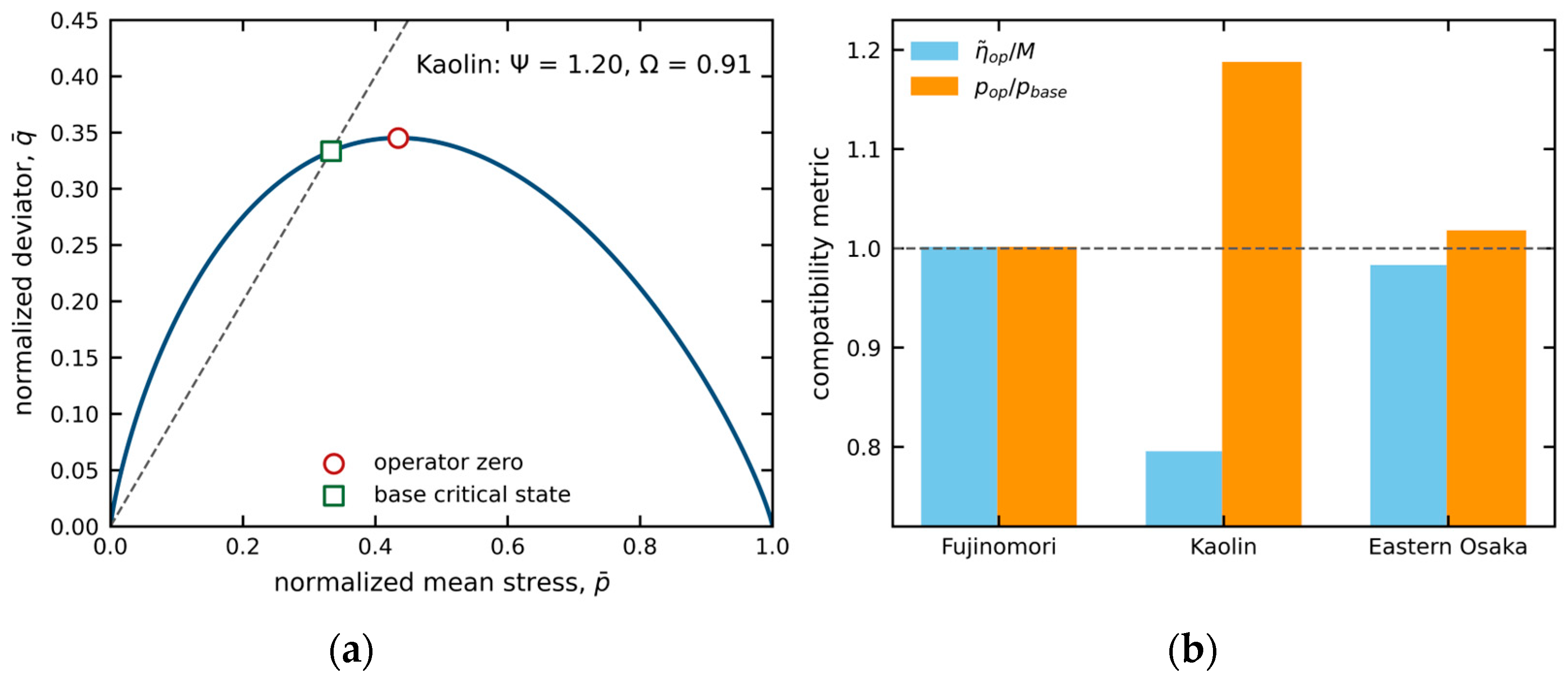
Figure 2.
A scalar counterexample to the ordinary local-chain substitute. The ordinate is the absolute difference between the exact and substituted values, divided by the absolute exact value, for the specified map and meridian. The marked value is 19.704% at . The calculation concerns operator composition; it is not an experimental error metric.
Figure 2.
A scalar counterexample to the ordinary local-chain substitute. The ordinate is the absolute difference between the exact and substituted values, divided by the absolute exact value, for the specified map and meridian. The marked value is 19.704% at . The calculation concerns operator composition; it is not an experimental error metric.
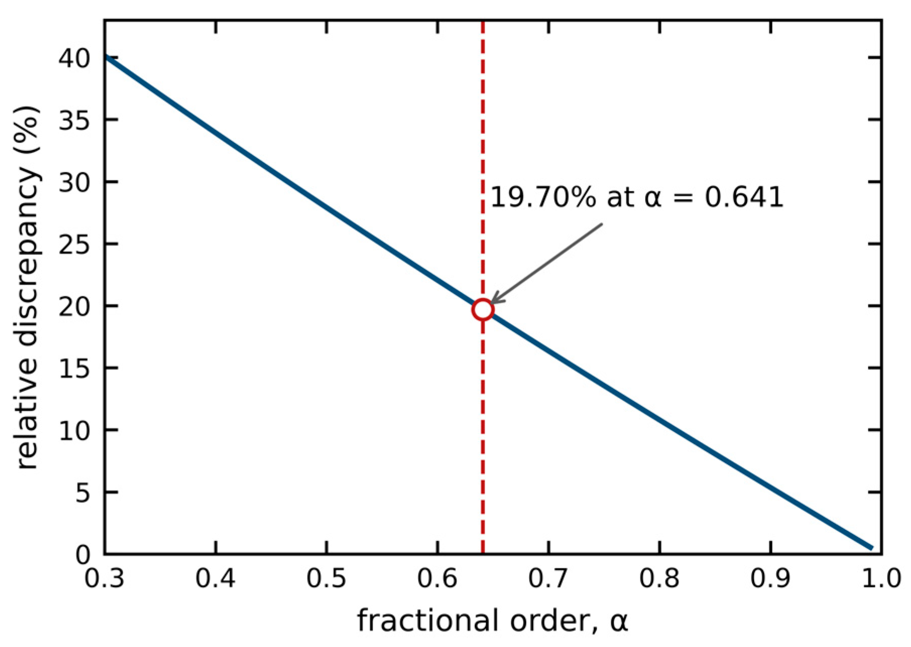
Figure 3.
Stress-locus agreement and numerical progression are different observables. (a) Digitized Fujinomori extension stresses and the common calculated normally consolidated locus. The dashed critical-state line is , with . (b) Real extension stress plotted against the internal loading coordinate for the two scalar embeddings. Dotted vertical lines mark first crossing of 99% of the analytical terminal, indicated by the horizontal dash-dot line. No measured strain is plotted against .
Figure 3.
Stress-locus agreement and numerical progression are different observables. (a) Digitized Fujinomori extension stresses and the common calculated normally consolidated locus. The dashed critical-state line is , with . (b) Real extension stress plotted against the internal loading coordinate for the two scalar embeddings. Dotted vertical lines mark first crossing of 99% of the analytical terminal, indicated by the horizontal dash-dot line. No measured strain is plotted against .
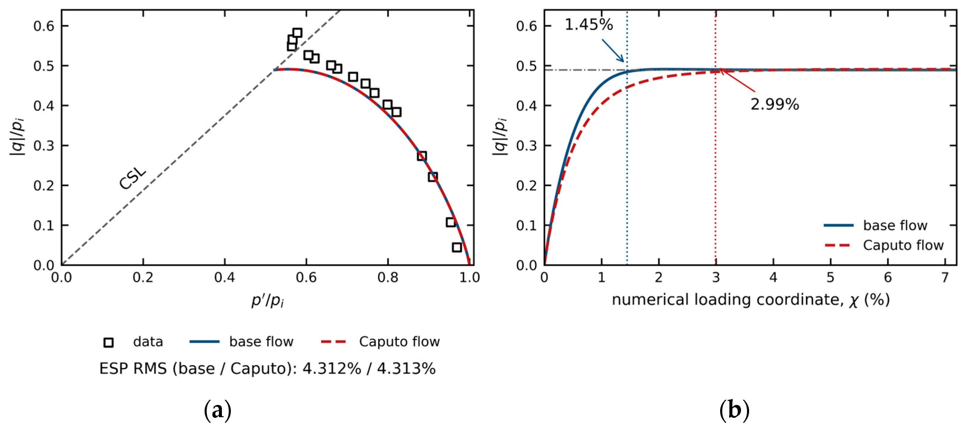
Figure 4.
Mechanisms behind the direct-substitution diagnostics for kaolin parameters. (a) F2 ties the sign-changing volumetric-flow candidate to the loading modulus, giving the same initial sign boundary for every plotted order. (b) The shear contribution compensates the negative volumetric contribution to the declared plastic work only above . These are boundaries of the specified equations, not measured material-failure envelopes.
Figure 4.
Mechanisms behind the direct-substitution diagnostics for kaolin parameters. (a) F2 ties the sign-changing volumetric-flow candidate to the loading modulus, giving the same initial sign boundary for every plotted order. (b) The shear contribution compensates the negative volumetric contribution to the declared plastic work only above . These are boundaries of the specified equations, not measured material-failure envelopes.
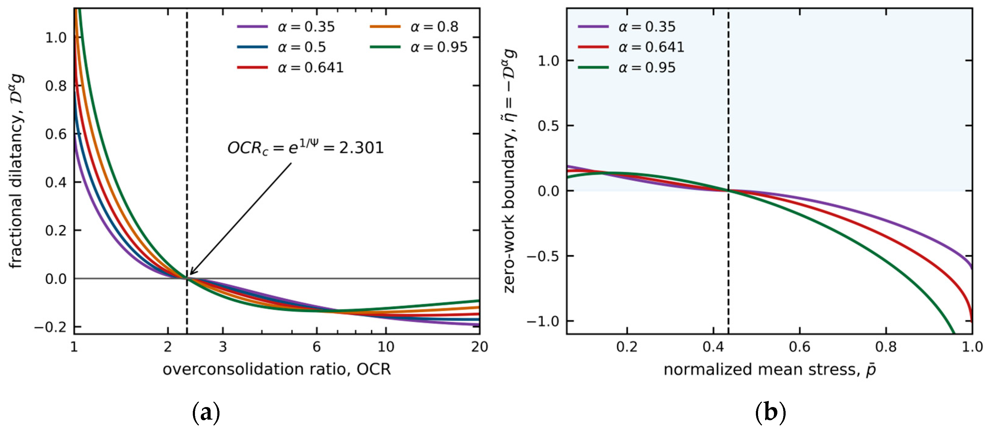
Figure 5.
Sensitivity of the two candidate terminal definitions to independent and . (a) Operator-terminal ratio . (b) Ratio of terminal surface coordinates . The latter is distinct from the NC mean-stress ratio in Table 3 because evolves during undrained loading. The black line is the coincidence condition. Rectangular colorbar end segments indicate values beyond the displayed interior levels.
Figure 5.
Sensitivity of the two candidate terminal definitions to independent and . (a) Operator-terminal ratio . (b) Ratio of terminal surface coordinates . The latter is distinct from the NC mean-stress ratio in Table 3 because evolves during undrained loading. The black line is the coincidence condition. Rectangular colorbar end segments indicate values beyond the displayed interior levels.
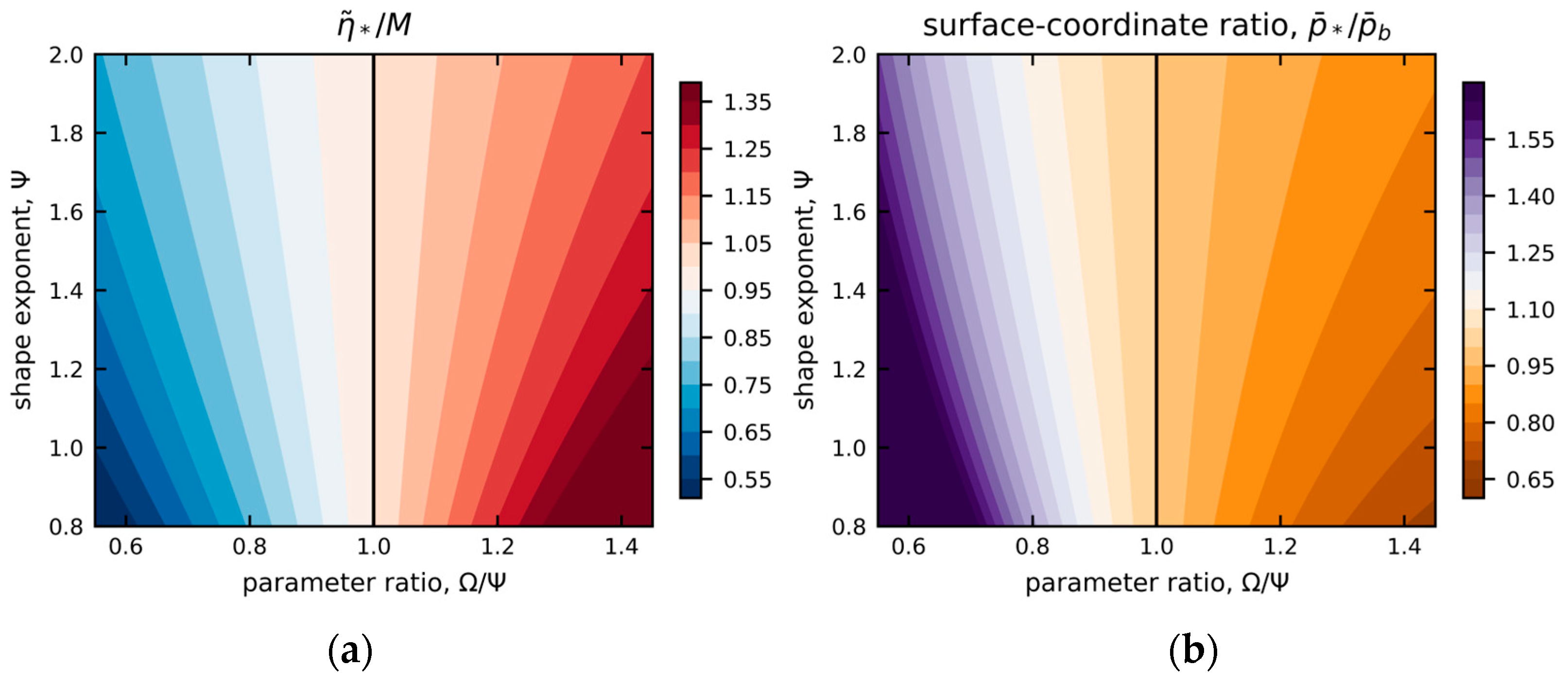

Table 1.
Constitutive questions separated in the present study and their evidential requirements.
| Question | Mathematical object | What can establish it | What cannot establish it |
| Coordinate composition | Scalar nonlocal integral | Invariant integration coordinate, terminal and kernel | Ordinary local Jacobian alone |
| Terminal compatibility | Surface stationary point versus material critical state | Equality of the two independently derived states | Calling both points ‘critical’ |
| Incremental consistency | Flow, hardening and plastic multiplier | Zero consistency rate and bounded surface residual | A fitted loading surface |
| Work and dissipation | Declared stress–plastic-coordinate pairing | Sign test for that pairing; energy model for physical dissipation | Convergence alone |
| Experimental validation | Complete parameterized response | Independent stress and strain observables | Replotting paths generated by another flow rule |
Table 2.
Inherited parameter sets and their roles in the audit.
| Clay | Source and context | Use here | |||||
| Fujinomori | 1.3615 | 0.0508 | 0.0112 | 1.20 | 1.20 | NC extension; digitized from [12] | Terminal + NC audit |
| Kaolin | 1.0500 | 0.1400 | 0.0500 | 1.20 | 0.91 | OCR 1, 1.2, 6, 10 [28,29,30] | Terminal + OC audit |
| Eastern Osaka | 1.2790 | 0.3550 | 0.0477 | 1.48 | 1.44 | Natural, structured clay [31] | Terminal audit only |
NC normally consolidated; OCR overconsolidation ratio. and are the numerical compression and swelling coefficients. For Fujinomori, Table 3 of [12] explicitly gives and , where and are void-ratio slopes. An additional specific-volume division would duplicate this normalization. For kaolin and Eastern Osaka, the supplied coefficient pairs are retained as audit inputs; their absolute laboratory-strain normalization is not established here. The terminal-pressure audit uses only their ratio, which is invariant under a common normalization.
Table 3.
Terminal-compatibility audit of the data-specific parameter sets.
| Clay | /(NC) | Real TE/TC at * | ||||
| Fujinomori | 1.00000 | 0.43460 | 0.43460 | 1.00000 | 0.68784 | 0.68784 |
| Kaolin | 0.79412 | 0.43460 | 0.33324 | 1.18616 | 0.78251 | 0.74074 |
| Eastern Osaka | 0.98166 | 0.50881 | 0.49935 | 1.01638 | 0.70496 | 0.70110 |
‘Real TE/TC at *’ is obtained by inverting the SMP mapping at . is the usual extension/compression criterion ratio evaluated at = . They are equal only when the operator terminal lies at = . TC and TE denote triaxial compression and extension; all deviatoric stresses in the extension comparisons are reported as non-negative magnitudes.
Table 4.
Fujinomori NC stress-locus error and numerical loading coordinate.
| Flow candidate | ESP RMS (%) | numerical (%) | independent (%) | |
| Base radial mapping | 4.31200 | 1.44511 | 1.44549 | 0.48908303 |
| Caputo, = 0.641 | 4.31311 | 2.98743 | 2.98886 | 0.48908303 |
ESP effective-stress path; initial mean effective stress. is the first crossing of 99% of the analytical terminal , using consecutive solver increments and linear interpolation. Independent values integrate along the exact NC locus (Appendix A). All values refer to the internal coordinate and are not laboratory-strain predictions.
Table 5.
Kaolin overconsolidated embedding diagnostics at = 0.641.
| OCR | Initial | F2 initial | F1 max | F1 min |
| 1.0 | 1.03148 | 9.93276 | +0.287648 | |
| 1.2 | 0.40956 | 3.94386 | +0.277312 | |
| 6.0 | -0.13135 | -1.26482 | -0.019047 | |
| 10.0 | -0.15165 | -1.46030 | -0.147487 |
Stresses are normalized by initial . F1 preserves the base loading modulus; F2 couples it to the substituted flow. Positive denotes an exterior state. The work rate uses Equation (5), pre-increment stress and the imposed increment . For OCR = 1, the initial operator is evaluated at . The general operator family does not have a finite value at for every order.
Disclaimer/Publisher’s Note: The statements, opinions and data contained in all publications are solely those of the individual author(s) and contributor(s) and not of MDPI and/or the editor(s). MDPI and/or the editor(s) disclaim responsibility for any injury to people or property resulting from any ideas, methods, instructions or products referred to in the content. |
© 2026 by the authors. Licensee MDPI, Basel, Switzerland. This article is an open access article distributed under the terms and conditions of the Creative Commons Attribution (CC BY) license (http://creativecommons.org/licenses/by/4.0/).
Copyright: This open access article is published under a Creative Commons CC BY 4.0 license, which permit the free download, distribution, and reuse, provided that the author and preprint are cited in any reuse.