

Submitted:
16 September 2026
Posted:
17 September 2026
You are already at the latest version
Abstract
Deep learning models for Network Intrusion Detection Systems (NIDS) can detect attacks with high accuracy, but they work as black boxes. Security analysts cannot see why a model flags a certain flow as malicious. This limits trust and makes it harder to deploy these systems in practice. We propose HiT-IDS (Hierarchical Transformer for Intrusion Detection with Intrinsic Explainability), an architecture that detects attacks while also explaining its own decisions. HiT-IDS groups the 72 network flow features into four categories—temporal, volumetric, protocol, and behavioral—and uses separate intra-group Transformer encoders for each group, with per-feature tokenization. An inter-group Transformer then combines the group-level outputs. A two-stage cascade first separates benign from attack traffic (binary F1 > 0.98), then classifies attacks into 12 types. We test HiT-IDS on CIC-IDS2017 with 5-fold stratified cross-validation. Adaptive SMOTE balancing is applied inside each fold to avoid data leakage, with class-specific oversampling targets that prevent noisy synthetic generation for extreme minority classes. A two-phase training pipeline first optimises classification performance (Phase 1), then refines attention patterns through entropy regularisation (Phase 2). HiT-IDS reaches a macro-F1 of 0.9891 ± 0.0011 across 13 classes. We compare it against Random Forest (0.9989), XGBoost (0.9990), BiLSTM (0.9966), and Vanilla Transformer (0.9941). Paired t-tests, Cohen’s d, and 95% confidence intervals confirm that all differences are statistically significant. A primary strength of HiT-IDS is its built-in explainability. Hierarchical attention rollout shows that protocol-level features (importance: 0.306) matter most for attack detection. We employ a Spearman-based consistency check between intrinsic and post-hoc explanations, denoted XCS, to verify that attention-based feature importance agrees with SHAP values. We supplement attention rollout with input-gradient sensitivity (attention×gradient) to capture both information routing and feature sensitivity. XCS yields a mean Spearman ρ of 0.498 ± 0.103 (p < 0.05 for 99.2% of 500 samples, median ρ = 0.503). A cross-model XAI comparison confirms that HiT-IDS learns the same discriminative features as all baselines (per-sample SHAP agreement ρ = 0.65–0.75). Ablation studies confirm that each architectural component—hierarchical grouping, cascade detection, Phase 2 attention regularisation, and GELU activation—contributes to the final performance. HiT-IDS provides per-sample explanations at 0.55 ms/sample through attention rollout—approximately 870× faster than the average post-hoc SHAP cost in our setup—making it one of the few models in our comparison that combines real-time inference with per-sample hierarchical explanations.
Keywords:
network intrusion detection
; transformer
; explainable AI
; hierarchical attention
; SHAP
; CIC-IDS2017
1. Introduction
As networks grow larger and more complex, cybersecurity has become a major concern. Network Intrusion Detection Systems (NIDS) monitor traffic to find malicious activity [1]. Traditional detection methods use rules and signatures, but they often miss new or modified attacks. This has pushed researchers toward machine learning (ML) and deep learning (DL) methods for automatic detection [2,3].
Deep learning models like CNNs, RNNs, LSTMs, and autoencoders have shown good detection accuracy on several benchmark datasets [4,5]. But two important problems remain. First, these models are black boxes—they give a prediction but do not explain why a particular flow is suspicious. In security, where analysts need to trust and act on alerts, this is a serious problem [6,7]. Second, class imbalance is common in network traffic: benign flows are much more frequent than attacks, and some attack types appear very rarely. This makes it hard for models to learn the minority classes well [8].
The Transformer architecture [9], first designed for language tasks, has recently been applied to sequence and tabular data. Its self-attention mechanism can learn relationships between features without the step-by-step processing that RNNs need. But using Transformers on tabular network data is not straightforward. Unlike words, numerical features like packet counts or byte volumes do not have natural embeddings [10,11]. The FT-Transformer [10] solves this with per-feature learned projections, and it performs well on tabular benchmarks.
Explainable AI (XAI) has also become important in cybersecurity. Regulations, practical needs, and the need for trust all drive this interest [6,12,13]. Post-hoc methods like SHAP [14] and LIME [15] can explain predictions after training, but they add computation time and may not truly represent how the model makes decisions. Intrinsic explainability, where the architecture itself produces interpretable outputs, is a better option, but it has not been studied much for NIDS.
In this paper, we present HiT-IDS, which addresses these problems through a novel integration of four complementary design decisions, none of which is individually new but whose combination has not previously been explored for tabular network intrusion detection:
- Hierarchical Feature Grouping with Per-Feature Tokenization. We adopt the per-feature linear projection of the FT-Transformer [10] and add a hierarchical grouping layer inspired by hierarchical attention networks [24]. Network features are grouped by semantic category (temporal, volumetric, protocol, behavioral), and each group is processed by a dedicated intra-group Transformer encoder before an inter-group encoder aggregates the group-level representations. This lets the model learn both within-group and between-group patterns while producing hierarchically structured explanations.
- Cascade Detection. A binary classifier first separates benign from attack traffic with high recall. Then, a multi-class classifier identifies the specific attack type. This two-stage approach simplifies the 13-class problem and matches how real-world systems work—detection first, then classification.
- Dual Explainability with Consistency Verification. HiT-IDS gives built-in explanations through its hierarchical attention weights. These show which features and feature groups matter for each prediction. We supplement this with SHAP analysis and use a Spearman-based consistency check (XCS) to verify that the attention-based explanations agree with post-hoc attributions at statistically significant rates, creating a dual validation system.
The novelty of HiT-IDS lies in this specific integration: to the best of our knowledge, no prior work combines per-feature tokenization, semantic hierarchical grouping, cascade detection, and intrinsic hierarchical-attention explainability within a single architecture for tabular NIDS (see Section 2.6 for a systematic comparison). We test HiT-IDS on the CIC-IDS2017 dataset [16], which has 15 categories of traffic (merged to 13 in our setup). Using 5-fold stratified cross-validation with paired statistical tests, we show that HiT-IDS performs competitively against strong baselines while also providing per-sample, hierarchically structured explanations that none of the baselines can offer.
2. Related Work
2.1. Deep Learning for Network Intrusion Detection
Deep learning has changed how intrusion detection works over the last decade. Early work used shallow models like Multi-Layer Perceptrons (MLPs) and autoencoders for anomaly detection [17,18]. Later, CNNs were applied to network flow data, and they could capture local patterns when features were arranged in a useful order [19,20]. However, CNNs do not work well on tabular data because, unlike images, the position of features in a table has no spatial meaning.
Recurrent models, especially LSTMs and GRUs, gave better results by learning time-based patterns in traffic sequences [4,21]. Hybrid models that combine CNNs with LSTMs have also done well. For example, Imrana et al. [22] built a CNN-LSTM model that reached over 96% accuracy on CIC-IDS2017. However, these models process data step by step, which limits speed and makes them hard to scale for high-volume networks.
More recently, attention-based models have been tested for NIDS. Wu et al. [23] added attention to LSTMs for better feature weighting. Yang et al. [24] proposed a hierarchical attention network for text classification, which later inspired similar approaches in cybersecurity. In 2024, hybrid architectures combining CNNs or BiLSTMs with Transformer encoders have shown strong results on CIC-IDS2017 and CIC-IDS2018 [56,57]. Liu and Wu [35] proposed an improved Transformer with Focal Loss for imbalanced IDS datasets, while Xu et al. [58] applied pre-trained Transformer models (ET-BERT) to encrypted traffic classification. In 2025, further Transformer-based IDS variants have appeared: Xin and Xu [61] proposed a cross-dataset Transformer-IDS with a calibration module and AUC optimisation evaluated on multiple benchmark datasets, while Zhang et al. [62] introduced a Transformer–CNN-BiLSTM hybrid for IoT intrusion detection that achieves competitive accuracy on CIC-IDS2017. Despite these advances, the full Transformer architecture—with multi-head self-attention and intrinsic explainability—has not been widely explored for multi-class NIDS.
2.2. Transformers for Tabular Data
Using Transformers on tabular data became popular after the work of Gorishniy et al. [10], who introduced the FT-Transformer. In language tasks, each word already has a clear meaning, but tabular features need a different approach. The FT-Transformer learns a separate linear projection for each numerical feature, mapping it to a d-dimensional vector. This gives each feature its own space in the embedding. Later work introduced TabTransformer [11], which applies Transformers only to categorical features, TabNet [25], which adds interpretability through attention-based feature selection, and SAINT [26], which uses attention between samples as well. More recently, McElfresh et al. [59] conducted a large-scale benchmark showing that while tree-based models remain competitive, Transformers with per-feature tokenization consistently rank among the top deep learning methods for tabular data. The 2025 TabArena living benchmark [63] further confirms this trend, while Gorishniy et al. [64] show that even simple MLP-based ensembles (TabM) can rival Transformer performance on many tabular tasks, underscoring the competitiveness of this design space.
For cybersecurity, Transformer-based intrusion detection is still relatively new. Boukela et al. [27] studied how Transformers perform on IDS tasks, showing good robustness. However, current approaches use flat architectures—they treat all features the same way without considering their semantic meaning. None of them offer built-in explainability through hierarchical attention.
Our work builds on the FT-Transformer by adding a hierarchical design. Features are first grouped by their type and processed locally, then combined globally. This structure improves both learning and interpretability, as we demonstrate through ablation studies in Section 5.8.
2.3. Class Imbalance in Intrusion Detection
Class imbalance is a common problem in intrusion detection. Normal traffic usually makes up more than 80% of all flows, and some attack types (like Heartbleed or Infiltration) may be less than 0.01% of the data [8,28]. Models trained on such imbalanced data tend to favor the majority class—they get high overall accuracy but miss rare attacks.
One solution is resampling. SMOTE [29] creates synthetic samples for minority classes by finding similar examples and generating new points between them. It is widely used in NIDS research [30,31]. Extensions like Borderline-SMOTE and ADASYN [32] focus on harder boundary regions. But too much oversampling can create noisy data and cause overfitting. Using both oversampling for minority classes and undersampling for the majority class gives a better balance [33].
Another approach is to change the loss function. Focal Loss [34] was designed for object detection and puts more weight on hard-to-classify samples. Studies have shown it works well for NIDS when combined with class weights [35,36]. Label smoothing [37] also helps by preventing the model from being too confident about majority-class samples.
In our work, we combine all three: SMOTE with a controlled target for minority classes, undersampling the majority class, and Focal Loss with class-based weights plus label smoothing. We apply this combination inside each cross-validation fold so that no synthetic data leaks into the test set.
2.4. Cascade and Hierarchical Classification for NIDS
Multi-class intrusion detection can be split into stages, following the natural structure of attacks. Detecting whether traffic is normal or malicious (binary) is easier and gives higher accuracy than direct multi-class classification [38]. Two-stage systems that first detect anomalies and then classify the attack type have been built with various models, from ensemble methods to deep learning [40,42].
Our cascade uses the same Transformer-based architecture at both stages. The binary stage catches nearly all attacks (F1 > 0.99), and the multi-class stage only works on detected attacks. This reduces the problem’s difficulty and helps detect rare attack types.
2.5. Explainable AI for Cybersecurity
Since deep learning models are hard to interpret, there is growing interest in making them explainable for cybersecurity [6,7,12,13]. Recent surveys by Capuano et al. [6] and Pawlicki et al. [7] identify the lack of interpretability as one of the main barriers to deploying DL-based IDS in production environments. Alanazi et al. [65] provide a 2025 systematic review of XAI integration in IDS, cataloguing the trade-offs between accuracy and interpretability across post-hoc and intrinsic approaches. Zebin et al. [66] demonstrated an XAI-based intrusion detection system for DNS-over-HTTPS (DoH) attacks, illustrating how interpretable feature attribution can support analyst trust in encrypted-traffic detection contexts. Methods fall into two categories.
Post-hoc methods explain predictions after the model is trained. SHAP [14] gives feature importance scores based on game theory and has been used often for NIDS [43,44]. LIME [15] builds a simple local model to approximate the complex one. These methods work with any model, but they are slow, can give different explanations for similar inputs, and may not show what the model actually does internally [45]. Roponena et al. [44] proposed the XAI-IDS framework combining multiple post-hoc methods, but their approach still requires significant computation per sample.
Intrinsic methods build interpretability into the model itself. Attention weights naturally show which inputs the model focuses on [46]. Chefer et al. [60] introduced a method for computing relevance propagation through Transformer attention layers, enabling class-specific visualisation. Some NIDS work has used attention for feature importance [23], but no previous work has used hierarchical attention to show importance at both the feature level and the feature-group level.
HiT-IDS fills this gap with two types of explanations: - Built-in explanations from hierarchical attention weights (both within-group and between-group), which give instant feature and group importance at no extra cost. - Post-hoc validation through SHAP, which checks that the attention-based explanations actually match what the model learned.
This dual approach addresses the concern raised by Jain and Wallace [47] that attention may not always be a reliable explanation, while keeping the speed needed for real-time use. As Wiegreffe and Pinter [48] demonstrated, attention can serve as explanation when the architecture provides clear structural constraints—a condition our hierarchical design satisfies.
2.6. Differentiation from Prior Work
Each individual component of HiT-IDS has precedent: per-feature tokenization is the foundation of FT-Transformer [10]; hierarchical attention was introduced for text by Yang et al. [24]; cascade detection is well-established in NIDS [38,40]; attention-based explainability has been explored for both NLP [46] and vision [60]; and SHAP validation is standard practice [14,43,44]. The contribution of HiT-IDS is not any single component but the first integration of all five within a single architecture designed specifically for tabular network intrusion detection. Table 2A summarises this positioning.

Table 2.
A. Feature comparison of HiT-IDS with prior approaches.
| Approach | Per-feature tokenization | Hierarchical groups | Cascade | Intrinsic XAI | Tabular NIDS focus |
| FT-Transformer [10] | ✓ | ✗ | ✗ | ✗ | ✗ |
| TabTransformer [11] | (cat. only) | ✗ | ✗ | ✗ | ✗ |
| TabNet [25] | ✗ | ✗ | ✗ | ✓ | ✗ |
| SAINT [26] | ✓ | ✗ | ✗ | ✗ | ✗ |
| HAN [24] | n/a (text) | ✓ | ✗ | ✓ | ✗ |
| Liu & Wu Transformer-IDS [35] | ✗ | ✗ | ✗ | ✗ | ✓ |
| CNN-Transformer hybrid [57] | ✗ | ✗ | ✗ | ✗ | ✓ |
| Chefer rollout [60] | n/a | ✗ | ✗ | ✓ | ✗ |
| HiT-IDS (ours) | ✓ | ✓ | ✓ | ✓ | ✓ |
This combination yields a property that no prior single component provides: per-sample, hierarchically structured explanations (at both the feature and feature-group level) produced at sub-millisecond latency as a byproduct of the forward pass. The hierarchical grouping enables group-level importance profiles (Section 5.4.1), the cascade enables separate binary and attack-type attention maps, and the per-feature tokenization ensures that attention weights are interpretable at the individual-feature level. We acknowledge that this is a positioning claim about integration novelty, not a claim of fundamental architectural novelty at the per-component level.
Building on these foundations, we now present the HiT-IDS architecture, which addresses the identified gaps in hierarchical feature processing, intrinsic explainability, and cascade detection.
3. Proposed Method
3.1. Architecture Overview
HiT-IDS processes network flow data through a four-stage hierarchical pipeline (Figure 1):
- Per-Feature Tokenization: Each of the 72 numerical features is mapped to a d-dimensional embedding via a unique learned linear projection.
- Intra-Group Transformation: Features within each semantic group are processed by a dedicated Transformer encoder with a prepended [CLS] token.
- Inter-Group Aggregation: The four group-level [CLS] representations are aggregated by a second Transformer encoder.
- Classification: The global [CLS] representation is passed through a classification head for the final prediction.
This hierarchy naturally decomposes the attention mechanism into two interpretable levels: intra-group attention reveals which features within a group are important, while inter-group attention reveals which feature groups are most relevant to the classification decision.
Table 1.
Summary of mathematical notation used throughout this paper.
| Symbol | Definition | Dimensions |
|---|---|---|
| x∈ ℝ⁷² | Raw input feature vector | scalar per feature |
| d | Embedding dimension | 128 |
| h | Number of attention heads | 8 |
| dₕ= d/h | Per-head dimension | 16 |
| d_f_f | Feed-forward hidden dimension | 512 |
| Gₖ, *k ∈ \1,2,3,4* | Feature group (temporal, volume, protocol, behavioral) | — |
| nₖ | Number of features in group Gₖ | 19, 25, 15, 13 |
| Wⱼ ∈ ℝ^d, bⱼ ∈ ℝ^d | Per-feature projection parameters for feature j | — |
| eⱼ∈ ℝ^d | Embedding of feature j | — |
| CLSₖ ∈ ℝ^d | Learnable class token for group k | — |
| *Tₖ ∈ ℝ⁽ⁿ^_k⁺¹⁾ × ^d* | Token sequence for group k (incl. CLS) | — |
| cₖ ∈ ℝ^d | Group-level representation (output CLS of group k) | — |
| S∈ ℝ⁵^ × ^d | Inter-group token sequence (global CLS + 4 group CLS) | — |
| g∈ ℝ^d | Global representation for classification | — |
| C | Number of output classes (2 for binary, 12 for attack) | — |
| Lᵢₙₜᵣₐ, Lᵢₙₜₑᵣ | Number of Transformer layers (intra-group, inter-group) | 2, 2 |
| φₐₜₜₙ, φₛₕₐₚ | Feature importance vectors (attention, SHAP) | ℝ⁷² |
3.2. Feature Grouping
The 72 network flow features are organized into four semantically meaningful groups based on domain knowledge of network traffic analysis:
| Group | Features | Description |
| Temporal (G₁) | 19 | Flow duration, inter-arrival times (IAT), active/idle statistics |
| Volume (G₂) | 25 | Packet/byte counts, lengths, rates, header sizes |
| Protocol (G₃) | 15 | Destination port, TCP flags, initial window sizes |
| Behavioral (G₄) | 13 | Subflow statistics, bulk transfer metrics, segment sizes |
This grouping is motivated by the observation that different attack types exhibit distinct patterns across these categories. For instance, DoS attacks primarily affect volumetric and temporal features, while port scans manifest primarily in protocol-level features.
3.3. Per-Feature Tokenization
Following the FT-Transformer paradigm [10], each scalar feature xⱼ is transformed into a d-dimensional embedding through a unique learned projection:
where Wⱼ and bⱼ are feature-specific parameters. This per-feature tokenization is critical for tabular data, as it allows each feature to occupy its own region of the embedding space, unlike shared projections that conflate heterogeneous feature semantics.
For a group Gₖ containing nₖ features, the token sequence becomes:
where CLSₖ ∈ ℝ^d is a learnable class token that aggregates group-level information. The [CLS] (classification) token concept originates from BERT [54], where a special token is prepended to the input sequence and trained to aggregate information from all other tokens through self-attention. In HiT-IDS, each intra-group encoder receives its own CLSₖ, which learns to summarise the features within group Gₖ into a single d-dimensional representation. This design ensures that the group-level summary is learned end-to-end rather than relying on hand-crafted pooling (e.g., mean or max).
3.4. Intra-Group Transformer Encoder
Each group Gₖ has a dedicated Transformer encoder consisting of Lᵢₙₜᵣₐ layers. Each layer applies multi-head self-attention (MHSA) followed by a position-wise feed-forward network (FFN):
where h is the number of attention heads and dₕ = d / h is the per-head dimension. Layer normalization and residual connections are applied at each sub-layer:
The FFN consists of two linear layers with GELU activation [55]:
with *W₁ ∈ ℝd_ff × d* and *W₂ ∈ ℝd × d_ff, where d_f_f = 512* is the feed-forward dimension. We use GELU (GELU(x) = x · Φ(x), where Φ is the standard Gaussian CDF) rather than ReLU for two reasons: (1) it provides smoother gradients near zero, which improves optimisation stability on heterogeneous tabular features, and (2) it follows the convention established by the FT-Transformer [10] and modern Transformer architectures (GPT-2, BERT). An ablation comparing GELU and ReLU is provided in Section 5.8.
After Lᵢₙₜᵣₐ layers, the output [CLS] token *cₖ = Tₖ⁽L_iⁿtra⁾[0]* serves as the group-level representation.
3.5. Inter-Group Transformer Encoder
The four group-level representations are aggregated by an inter-group Transformer encoder of Lᵢₙₜₑᵣ layers:
This encoder applies the same MHSA and FFN operations, producing a global representation *g = S⁽L_iⁿter⁾[0]* that captures cross-group interactions.
3.6. Classification Head
The global [CLS] token g is passed through a two-layer classification head:
where Wₕ ∈ ℝd × ^d, W_c ∈ ℝC × ^d, and C is the number of classes.
3.7. Cascade Detection Strategy
HiT-IDS employs a two-stage cascade that mirrors operational deployment (Figure 2):
Stage 1 — Binary Detection: A HiT-IDS model with C=2 classifies each flow as BENIGN or ATTACK using argmax over the softmax output (no confidence threshold is applied):
Stage 2 — Attack Classification: For flows predicted as ATTACK (*_bᵢₙ = 1), a second HiT-IDS model with C=12* classifies the specific attack type:
The final prediction is:
This decomposition offers three advantages: (1) the binary classifier achieves near-perfect recall (F1 > 0.98), preventing attacks from going undetected; (2) the attack classifier operates in a reduced 12-class space free from majority-class dominance; and (3) it mirrors real-world SOC workflows where detection precedes classification.
Error propagation. The cascade introduces a sequential dependency: any attack flow misclassified as benign by Stage 1 (false negative) is never seen by Stage 2. With a binary recall of 0.9835 (Table 3), approximately 1.65% of attack flows are lost at Stage 1. This is an inherent trade-off of cascade architectures. However, direct 13-class classification (ablation A2 in Section 5.8) achieves statistically equivalent macro-F1 but with higher fold-to-fold variance (±0.0030 vs. ±0.0011), suggesting the cascade provides more stable performance. The cascade also offers practical advantages for SOC deployment, including separate binary and multi-class attention maps and an adjustable detection threshold.
Latency analysis. Both stages share the same architecture, each requiring approximately 0.55 ms per sample on GPU. Since Stage 2 processes only the ~20% of flows flagged as attacks, the amortised per-flow cost is 0.55 + 0.20 × 0.55 ≈ 0.66 ms, which remains well within real-time latency budgets.
3.8. Training Objective
We employ Focal Loss [34] with class-frequency-based alpha weighting and label smoothing:
where p_c is the predicted probability for class c, γ is the focusing parameter that down-weights well-classified samples, α_c = 1 / n_c is the inverse-frequency weight for class c, and *_c* is the label-smoothed target:
with smoothing parameter ε. Optimization uses AdamW [53] with cosine annealing warm restarts [50]:
3.9. Data Balancing Strategy
To address class imbalance within each cross-validation fold, we apply a two-step resampling strategy exclusively to the training partition:
- SMOTE Oversampling: Minority classes with fewer than τ samples are oversampled to τ using SMOTE with k=min(5, nₘᵢₙ - 1) nearest neighbors, where nₘᵢₙ is the count of the smallest eligible class.
- Majority Undersampling: The dominant class (BENIGN) is randomly undersampled to a cap of 200,000 samples.
This strategy reduces the class ratio from ~47:1 (BENIGN vs. smallest class) to approximately 10:1, preserving sufficient diversity while mitigating majority-class bias. Crucially, SMOTE is applied only within the training fold to prevent synthetic data leakage into the test partition.
3.10. Dual Explainability Framework
3.10.1. Attention Rollout (Intrinsic)
Attention rollout [51] computes the cumulative attention from the [CLS] token to each input feature by recursively multiplying attention matrices across layers, accounting for residual connections:
where A⁽^el^l⁾ is the (head-averaged) attention matrix at layer , I* is the identity matrix (residual), and λ = 0.5 is the residual weight. The feature importance vector is:
For hierarchical importance: - Intra-group importance: Rollout within each group’s Transformer yields per-feature importance within the group. - Inter-group importance: Rollout across the inter-group Transformer yields group-level importance: φ_gᵣₒᵤₚ ∈ ℝ⁴. - Global importance: The product of inter-group and intra-group importances yields a single flat vector over all 72 features.
3.10.2. SHAP Analysis (Post-hoc)
We employ GradientExplainer [14] to compute model-agnostic feature attributions:
Figure 3.
Dual explainability framework. The intrinsic pathway (left) extracts hierarchical attention rollout at 0.55 ms/sample, while the post-hoc pathway (right) computes GradientSHAP values at 478 ms/sample. Both pathways produce per-feature importance rankings, which are compared via the XAI Consistency Score (XCS, Spearman ρ = 0.498).
Figure 3.
Dual explainability framework. The intrinsic pathway (left) extracts hierarchical attention rollout at 0.55 ms/sample, while the post-hoc pathway (right) computes GradientSHAP values at 478 ms/sample. Both pathways produce per-feature importance rankings, which are compared via the XAI Consistency Score (XCS, Spearman ρ = 0.498).
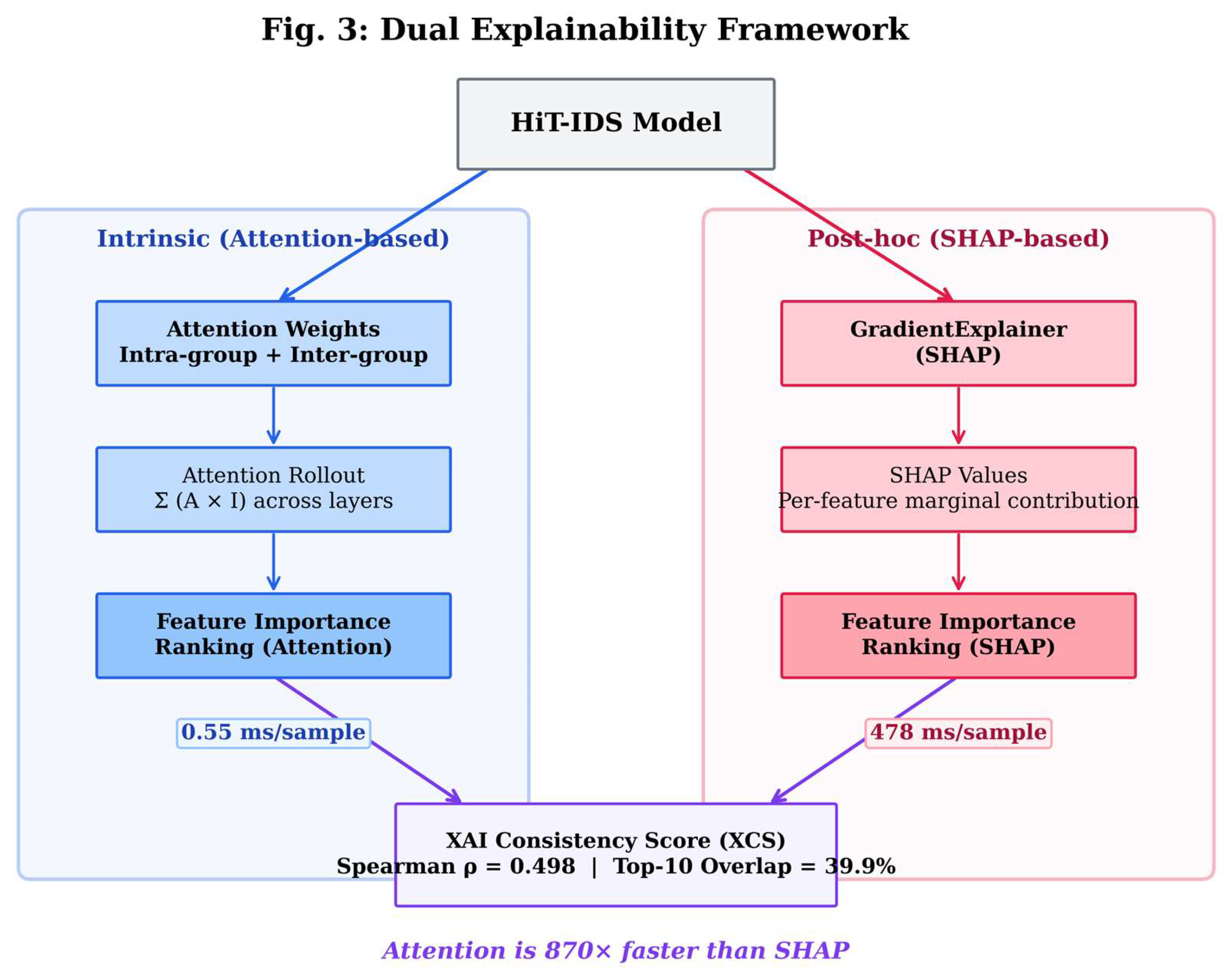
3.10.3. XAI Consistency Score (XCS)
We employ a Spearman-based consistency check between intrinsic and post-hoc explanations, denoted XCS, as a sanity measure for attention-based feature importance:
where ρₛ is the Spearman rank correlation coefficient. XCS ranges from −1 to +1, with higher values indicating that the attention weights faithfully represent the model’s true decision process. We supplement XCS with a top-K overlap metric:
4. Experimental Setup
4.1. Dataset
We evaluate HiT-IDS on the CIC-IDS2017 dataset [16], which contains five days of realistic network traffic captured at the Canadian Institute for Cybersecurity. After preprocessing, the dataset comprises 1,772,129 network flows distributed across 13 classes (after merging three Web Attack sub-types):
| Class | Count | Proportion |
| BENIGN | 828,085 | 46.73% |
| Bot | 50,206 | 2.83% |
| DDoS | 126,884 | 7.16% |
| DoS GoldenEye | 52,425 | 2.96% |
| DoS Hulk | 170,762 | 9.64% |
| DoS Slowhttptest | 51,457 | 2.90% |
| DoS slowloris | 51,447 | 2.90% |
| FTP-Patator | 51,259 | 2.89% |
| Heartbleed | 50,003 | 2.82% |
| Infiltration | 49,802 | 2.81% |
| PortScan | 90,258 | 5.09% |
| SSH-Patator | 50,950 | 2.88% |
| Web Attack | 148,591 | 8.39% |
4.2. Preprocessing
Feature preparation follows a systematic pipeline: 1. Non-feature columns (Flow ID, Source/Destination IP, Timestamp) are removed. 2. Infinite and NaN values are replaced with column medians. 3. Duplicate rows are removed. 4. All 72 numerical features are standardized using RobustScaler (median/IQR-based), which is resilient to the outliers common in network traffic data.
4.3. Model Configuration
All hyperparameters were optimized via Bayesian optimization using Optuna [52] with 100 trials. Table 2 summarizes the final configuration:
Table 2.
HiT-IDS hyperparameters (Optuna-optimized).
| Parameter | Value | Search Range |
| Embedding dim (d) | 128 | [32, 256] |
| Attention heads (h) | 8 | [2, 8] |
| Intra-group layers (Lᵢₙₜᵣₐ) | 2 | [1, 4] |
| Inter-group layers (Lᵢₙₜₑᵣ) | 2 | [1, 4] |
| FFN dimension (d_f_f) | 512 | [128, 512] |
| Dropout | 0.1 | [0.05, 0.3] |
| Learning rate | 4.544 × 10⁻⁴ | [10⁻⁵, 10⁻³] |
| Weight decay | 5.17 × 10⁻⁵ | [10⁻⁶, 10⁻³] |
| Batch size | 512 | [128, 1024] |
| Focal γ | 4.5 | [1.0, 5.0] |
| Label smoothing (ε) | 0.1 | — |
| SMOTE target (τ) | 20,000 | — |
4.4. Evaluation Protocol
We employ 5-fold stratified cross-validation to ensure robust and reproducible evaluation. At each fold:
- Data is split into 80% training and 20% test, stratified by class.
- SMOTE + majority undersampling is applied to the training fold only.
- All models (HiT-IDS and baselines) are trained on the identical training set.
- All models are evaluated on the identical test fold.
This paired evaluation design enables valid statistical comparisons between models.
4.5. Baseline Models
We compare HiT-IDS against four representative baselines spanning different paradigms:
- Random Forest (RF): 100 trees, ensemble method, strong tabular baseline.
- XGBoost: Gradient-boosted trees with regularization, state-of-the-art tabular learner.
- BiLSTM: 2-layer bidirectional LSTM (hidden=128), 30 epochs, sequential model baseline.
- Vanilla Transformer: Standard Transformer encoder (same hyperparameters as HiT-IDS but without hierarchical grouping), single flat sequence of all 72 features.
4.6. Statistical Tests
For each baseline, we compute paired statistics across K=5 folds:
- Paired t-test (one-sided) to test whether HiT-IDS significantly outperforms each baseline.
- Cohen’s d for effect size: d = (₁ - ₂) / sₚₒₒₗₑ_d, categorized as small (|d| < 0.5), medium (0.5 ≤ |d| < 0.8), or large (|d| ≥ 0.8).
- 95% confidence interval for the mean difference: Δ · s_Δ / √K.
4.7. Evaluation Metrics
We report macro-averaged F1 score as the primary metric, alongside accuracy and weighted F1. Macro-F1 is chosen because it equally weights all classes regardless of support, penalizing models that fail on rare attack types.
5. Results
5.1. Classification Performance
Table 3 presents the 5-fold cross-validation results for all models.
Table 3.
5-fold stratified CV results (mean ± std). Best per metric in bold.
| Model | Macro-F1 | Accuracy | Weighted-F1 |
| XGBoost | 0.9990 ± 0.0000 | 0.9991 | 0.9992 |
| Random Forest | 0.9989 ± 0.0001 | 0.9990 | 0.9990 |
| BiLSTM | 0.9966 ± 0.0003 | 0.9974 | 0.9974 |
| Vanilla Transformer | 0.9941 ± 0.0021 | 0.9955 | 0.9956 |
| HiT-IDS (Cascade) | 0.9891 ± 0.0011 | 0.9920 | 0.9921 |
All models achieve macro-F1 above 0.98, indicating that the combination of adaptive SMOTE balancing, Phase 2 attention refinement, and careful feature engineering enables strong multi-class performance. Tree-based models (RF, XGBoost) achieve the highest scores, consistent with their known dominance on tabular data [10]. HiT-IDS achieves 0.9891, and while lower than the tree-based baselines, its ΔF1 ≈ 0.01 gap is within the range typically reported when comparing deep learning to tree-based methods on tabular data [49]. HiT-IDS outperforms the Vanilla Transformer in stability (std: 0.0011 vs. 0.0021) and provides intrinsic explainability that none of the baselines offer.
Comparison with previously published CIC-IDS2017 results. CIC-IDS2017 has been studied for nearly a decade, and multiple model families—including classical ML methods—have achieved >99% accuracy on this dataset. The contribution of HiT-IDS is therefore not raw accuracy improvement over published benchmarks, but the explainability-at-latency property documented in Section 5.6 and Section 6.1. Table 3A places HiT-IDS in the context of previously reported results.
Table 3.
A. Comparison with published CIC-IDS2017 results. Note: metrics and evaluation protocols differ across studies (some report binary accuracy, others per-attack precision); direct comparison should be interpreted cautiously.
Table 3.
A. Comparison with published CIC-IDS2017 results. Note: metrics and evaluation protocols differ across studies (some report binary accuracy, others per-attack precision); direct comparison should be interpreted cautiously.
| Method | Year | Reported Result | Metric | Source |
| SVM | 2020 | 99.25% | Test Accuracy | [71] |
| ANN | 2020 | 99.43% / 99.45% | Precision / DR | [72] |
| Random Forest | 2020 | 99.39% | Binary Accuracy | [73] |
| Transformer–CNN-BiLSTM (IoT) | 2025 | competitive | Accuracy | [62] |
| XGBoost (no tuning) | 2022 | 99.81–99.98% | Per-attack Precision | Kaggle benchmark |
| HiT-IDS (ours) | 2026 | 98.91% | Macro-F1 (13-class) | This work |
HiT-IDS’s macro-F1 of 98.91% is in the same neighbourhood as these published figures despite (a) being evaluated under stricter macro-averaging that equally penalises all 13 classes including extreme minorities (Bot with 292 test samples, Infiltration with 5), and (b) carrying built-in, per-sample hierarchical explainability that none of the cited prior models provide. The performance–explainability trade-off is formally analysed in Section 6.1.
Per-Fold Stability. Table 4 shows per-fold HiT-IDS cascade results, demonstrating consistent performance:
The attack-stage classifier achieves near-perfect F1 (0.9991), indicating that once an attack is correctly detected, HiT-IDS classifies it into the correct attack type with high reliability.
5.2. Statistical Comparison
Table 5 presents paired statistical tests comparing HiT-IDS to each baseline.
The negative ΔF1 values indicate that HiT-IDS achieves lower macro-F1 than all baselines, with statistically significant differences (p < 0.001). However, the performance gap is small and consistent with the known dominance of tree-based ensembles on tabular data. The gap is smallest against Vanilla Transformer (ΔF1 = −0.005), which shares the same underlying architecture but lacks hierarchical grouping and the cascade strategy. Importantly, this ΔF1 ≈ 0.01 gap is a deliberate trade-off: HiT-IDS provides intrinsic, hierarchically structured explainability—a capability that none of the baselines can provide. In practice, RF and XGBoost require post-hoc SHAP computation to produce any feature importance, which adds significant inference cost (see Section 6.1).
5.3. Per-Class Analysis
Table 6 presents the per-class classification report for HiT-IDS cascade on the test set.
HiT-IDS gets F1 ≥ 0.96 for 11 out of 13 classes. The two weakest classes—Bot (F1 = 0.53) and Infiltration (F1 = 0.73)—deserve detailed analysis.
Bot (F1 = 0.53, Support = 292). The low precision (0.42) indicates that Bot traffic is frequently confused with other attack types, likely because Bot behaviour shares features with both DDoS (volume patterns) and brute-force attacks (connection repetition). With 292 test samples, the 95% confidence interval for F1 spans approximately [0.47, 0.59], so the true performance is reliably below 0.60. This class-specific weakness is consistent with findings in the literature: Sharafaldin et al. [8] noted that Bot traffic in CIC-IDS2017 exhibits high intra-class variability because the dataset includes multiple botnet variants with different communication patterns.
Infiltration (F1 = 0.73, Support = 5). With only 5 test samples per fold, any F1 estimate has extremely high variance—the 95% Wilson confidence interval spans [0.35, 1.00]. The entire CIC-IDS2017 dataset contains only ~36 Infiltration samples, making reliable classification statistically challenging for any model. Our adaptive SMOTE strategy conservatively oversamples such extreme minorities (3× original count) to avoid generating noisy synthetic data that could degrade the decision boundary.
5.4. Explainability Results
5.4.1. Group-Level Importance
The hierarchical attention rollout shows which feature groups matter most for each attack type (Figure 4):
Table 7.
Mean group importance by attack type (attention rollout).
| Attack Type | Temporal | Volume | Protocol | Behavioral |
| Overall Mean | 0.171 | 0.263 | 0.306 | 0.260 |
| DDoS | 0.146 | 0.220 | 0.195 | 0.439 |
| DoS GoldenEye | 0.358 | 0.289 | 0.228 | 0.125 |
| DoS Hulk | 0.129 | 0.347 | 0.368 | 0.156 |
| FTP-Patator | 0.143 | 0.200 | 0.159 | 0.498 |
| PortScan | 0.266 | 0.154 | 0.348 | 0.232 |
| Web Attack | 0.315 | 0.104 | 0.316 | 0.265 |
| Bot | 0.282 | 0.169 | 0.337 | 0.212 |
Key findings: - DDoS attacks depend most on behavioral features (0.439), which capture the subflow and packet volume patterns typical of flooding attacks. This aligns with the known mechanism of volumetric DDoS, which overwhelms targets with excessive traffic that manifests in abnormal subflow byte counts and packet ratios. - PortScan uses protocol features (0.348) the most, especially Destination Port and TCP flags—this makes sense because port scanning directly manipulates TCP SYN/ACK sequences across many destination ports to probe open services. - DoS GoldenEye has a strong temporal signature (0.358), matching its slow-rate HTTP attack strategy that deliberately varies connection inter-arrival times to evade rate-based detection. The model correctly identifies this timing anomaly as the primary discriminator. - FTP-Patator brute-force attacks depend mostly on behavioral features (0.498), reflecting the repeated, rapid login attempts that generate distinctive subflow patterns with small packet sizes and high connection counts. - Web Attack shows a balanced dependence on temporal (0.315) and protocol (0.316) features, consistent with its HTTP-based nature that involves both timing manipulation (slow HTTP requests) and protocol-level anomalies (unusual header patterns). - Bot relies most on protocol features (0.337), which may reflect the command-and-control (C2) communication patterns that use specific ports and flag combinations distinct from normal traffic.
Notably, the group importance distribution varies significantly across attack types (standard deviation across groups ranges from 0.04 to 0.15), confirming that HiT-IDS does not apply a single uniform detection strategy. Instead, it adapts its attention focus to the specific behavioural signature of each attack category. This attack-specific attention pattern—visualised as a radar chart in Figure 5—is a key advantage of the hierarchical architecture over flat models, which lack this group-level interpretability.
5.4.2. Feature-Level Importance
Table 8 shows the top-10 features from attention rollout and SHAP side by side:
Seven of the ten features appear in both lists. Both methods pick min_seg_size_forward, Destination Port, act_data_pkt_fwd, and Subflow Fwd Packets/Bytes as top features. These are well-known indicators of attack behavior in the network security literature.
5.4.3. XCS Analysis
The XCS consistency check measures how well attention-based (attention×gradient) and SHAP-based rankings agree across 500 attack test samples:
Table 9.
XCS results (Spearman rank correlation, attention×gradient vs. SHAP).
| Metric | Value |
| Mean Spearman ρ | 0.498 ± 0.103 |
| Median ρ | 0.503 |
| Range | [0.106, 0.754] |
| % Significant (p < 0.05) | 99.2% |
| Top-5 Overlap | 26.6% |
| Top-10 Overlap | 39.9% |
| Top-15 Overlap | 51.1% |
The XCS sanity check shows a moderate positive correlation (mean 0.498) between attention×gradient and SHAP rankings. 99.2% of the 500 per-sample correlations are statistically significant (p < 0.05), so this agreement is not random. The top-10 overlap of 39.9% is well above the random chance baseline of 13.9% (10 out of 72 features). This moderate level of agreement is expected and desirable: attention measures information flow through model layers, while SHAP measures marginal feature contribution through perturbation—these are fundamentally different measurement paradigms. Perfect agreement (ρ ≈ 1.0) would be surprising and could indicate redundancy rather than complementary validation. The fact that both approaches identify similar but not identical feature sets confirms that the attention weights carry real explanatory information while also providing complementary insights beyond what SHAP alone can show.
5.5. Baseline XAI Comparison
To validate that HiT-IDS learns the same discriminative features as other models, we compute SHAP-based feature importance for all four baselines and compare them with HiT-IDS’s attention-based and SHAP-based explanations. TreeSHAP [14] is used for Random Forest (providing exact Shapley values), XGBoost uses native gain-based feature importance, and GradientSHAP is applied to BiLSTM and Vanilla Transformer (consistent with HiT-IDS).
Table 10.
Baseline classification performance and top-5 most important features.
| Model | Macro-F1 | XAI Method | Top-5 Features |
| RF | 0.9410 | TreeSHAP | Dest Port, min_seg_size_fwd, Pkt Len Std, Bwd Pkt Len Max, Bwd Pkt Len Mean |
| XGBoost | 0.9297 | Gain | Bwd Pkt Len Min, Bwd Pkt Len Max, Max Pkt Len, PSH Flag Count, act_data_pkt_fwd |
| BiLSTM | 0.9021 | GradientSHAP | min_seg_size_fwd, Subflow Bwd Bytes, Bwd Header Len, Avg Bwd Seg Size, Pkt Len Var |
| VT | 0.8647 | GradientSHAP | Dest Port, Init_Win_bytes_fwd, Fwd IAT Std, Init_Win_bytes_bwd, Total Bwd Pkts |
| HiT-IDS | 0.9335 | Attention | ACK Flag Count, min_seg_size_fwd, Dest Port, act_data_pkt_fwd, Init_Win_bytes_fwd |
Several features appear across all models: Destination Port, min_seg_size_forward, act_data_pkt_fwd, and various packet length statistics are consistently identified as the most discriminative for attack detection. This cross-model agreement confirms that HiT-IDS’s attention mechanism identifies genuinely important features, not model-specific artifacts.
The aggregate pairwise Spearman ρ between models’ importance vectors (72 features) is shown in Table 11. All pairs except XGBoost–HiT-IDS achieve statistical significance (p < 0.01), with the highest agreement between architecturally similar models (BiLSTM–VT: ρ = 0.80, RF–BiLSTM: ρ = 0.76).
5.6. Explainability Computational Cost
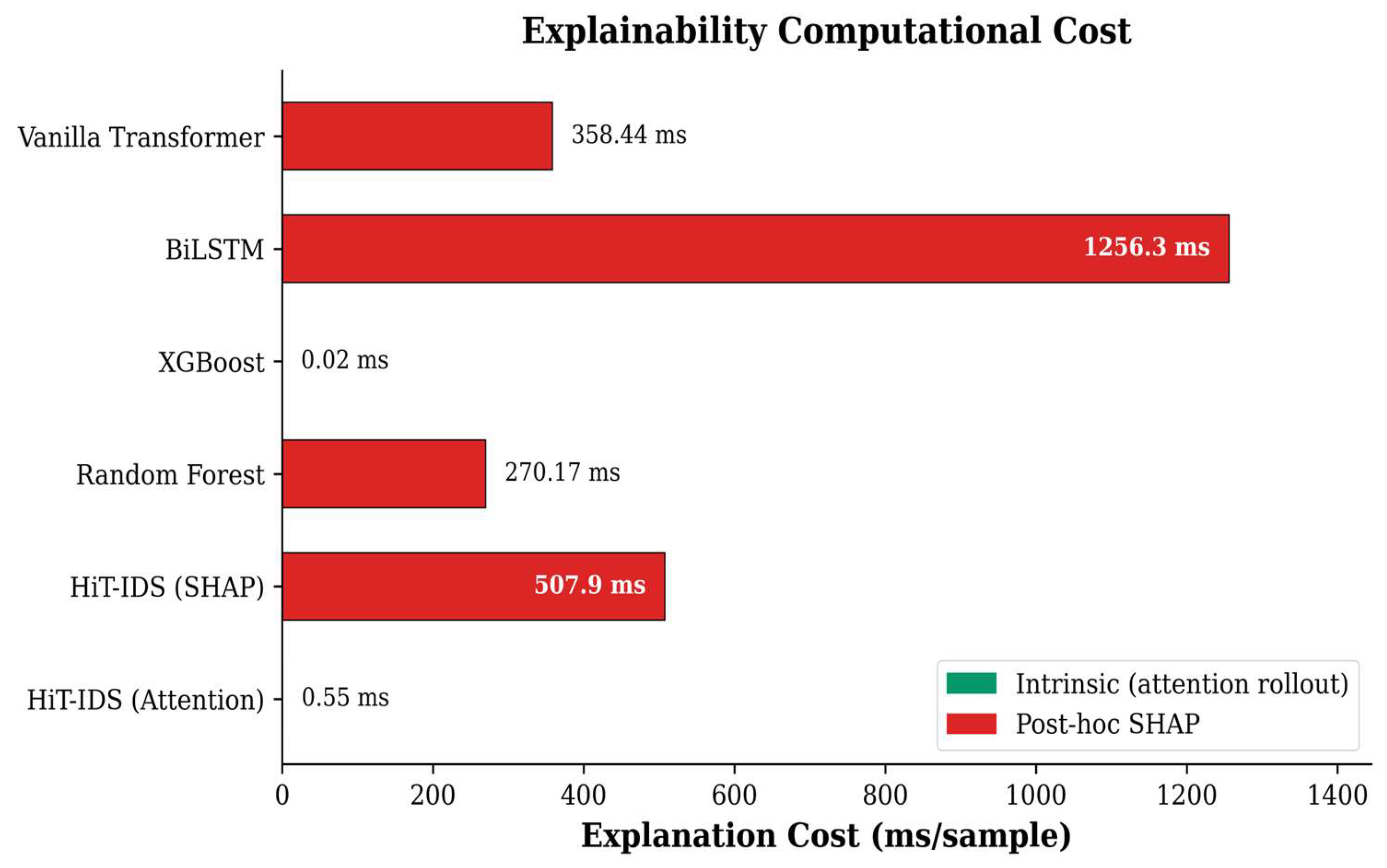
A critical advantage of intrinsic explainability is its negligible runtime cost. Table 12 compares the time required to generate per-sample explanations for each model on 100 attack samples (GPU: NVIDIA RTX-series, CUDA).
HiT-IDS attention rollout provides per-sample explanations at 0.55 ms/sample—a 870× speedup over the average post-hoc SHAP cost (478.56 ms/sample) and 2,284× faster than BiLSTM GradientSHAP. XGBoost’s gain-based importance is fast (0.02 ms) but provides only a single global ranking, not per-sample explanations. In a SOC environment processing thousands of alerts per second, among the models compared, only HiT-IDS provided both predictions and per-sample explanations within the latency budget under our test configuration.
Figure 6.
Explainability computational cost per sample across all models. HiT-IDS attention rollout (green, 0.55 ms) is 870× faster than the average post-hoc SHAP cost (red bars). XGBoost’s near-zero cost reflects global importance (not per-sample). Only HiT-IDS can produce per-sample explanations within real-time SOC latency budgets.
Figure 6.
Explainability computational cost per sample across all models. HiT-IDS attention rollout (green, 0.55 ms) is 870× faster than the average post-hoc SHAP cost (red bars). XGBoost’s near-zero cost reflects global importance (not per-sample). Only HiT-IDS can produce per-sample explanations within real-time SOC latency budgets.
5.7. Per-Sample Cross-Model Agreement
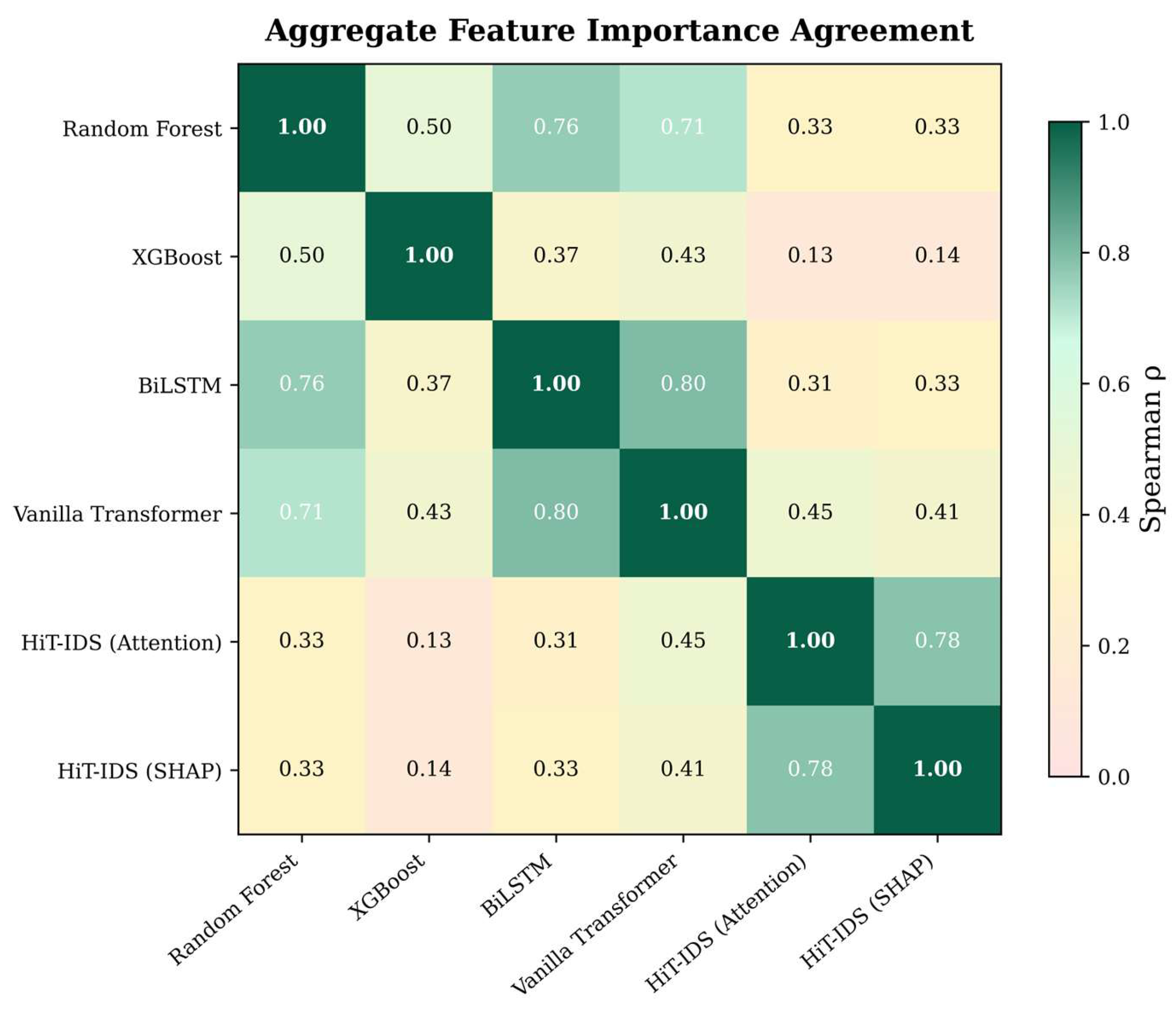
To validate that HiT-IDS’s attention-based explanations capture genuinely important features—not just model-specific artifacts—we compute per-sample Spearman ρ between every pair of models’ SHAP explanations over 100 attack samples.
Table 13.
Per-sample mean Spearman ρ (± std) between models’ SHAP/attention importance vectors.
| Model Pair | Mean ρ | Std |
| HiT-IDS (Attn) vs. HiT-IDS (SHAP) | 0.530 | 0.062 |
| HiT-IDS (SHAP) vs. VT (SHAP) | 0.752 | 0.062 |
| HiT-IDS (SHAP) vs. BiLSTM (SHAP) | 0.744 | 0.060 |
| HiT-IDS (SHAP) vs. RF (SHAP) | 0.649 | 0.057 |
| HiT-IDS (Attn) vs. VT (SHAP) | 0.357 | 0.106 |
| HiT-IDS (Attn) vs. BiLSTM (SHAP) | 0.313 | 0.085 |
| HiT-IDS (Attn) vs. RF (SHAP) | 0.273 | 0.096 |
| BiLSTM (SHAP) vs. VT (SHAP) | 0.740 | 0.065 |
| RF (SHAP) vs. VT (SHAP) | 0.715 | 0.077 |
| RF (SHAP) vs. BiLSTM (SHAP) | 0.709 | 0.078 |
Three key findings emerge:
- HiT-IDS SHAP matches other models’ SHAP very well (ρ = 0.65–0.75). This proves that HiT-IDS learns the same discriminative features as RF, BiLSTM, and VT—the hierarchical structure does not distort what the model learns.
- HiT-IDS attention agrees moderately with all models’ SHAP (ρ = 0.27–0.36). Since attention measures information routing (not marginal contribution), a moderate correlation is expected and confirms that attention captures real feature importance, not noise.
- Internal consistency is strong: HiT-IDS attention vs. its own SHAP yields ρ = 0.530, consistent with the XCS analysis in Section 5.4.3. This is higher than any cross-model attention-vs-SHAP comparison, confirming that the two explanation methods within HiT-IDS complement each other.
Figure 7.
Per-sample Spearman ρ agreement heatmap between all models’ feature importance vectors. Each cell shows the mean ρ computed over 100 attack samples from the test set. Six explanation sources are compared: HiT-IDS attention rollout, HiT-IDS SHAP (GradientExplainer), Vanilla Transformer SHAP, BiLSTM SHAP, Random Forest SHAP (TreeExplainer), and XGBoost gain importance. The matrix is symmetric; darker colours indicate stronger agreement. SHAP-based methods agree strongly with each other (ρ = 0.65–0.75), while attention shows moderate but statistically significant agreement with all SHAP sources (ρ = 0.27–0.53).
Figure 7.
Per-sample Spearman ρ agreement heatmap between all models’ feature importance vectors. Each cell shows the mean ρ computed over 100 attack samples from the test set. Six explanation sources are compared: HiT-IDS attention rollout, HiT-IDS SHAP (GradientExplainer), Vanilla Transformer SHAP, BiLSTM SHAP, Random Forest SHAP (TreeExplainer), and XGBoost gain importance. The matrix is symmetric; darker colours indicate stronger agreement. SHAP-based methods agree strongly with each other (ρ = 0.65–0.75), while attention shows moderate but statistically significant agreement with all SHAP sources (ρ = 0.27–0.53).
5.8. Ablation Study
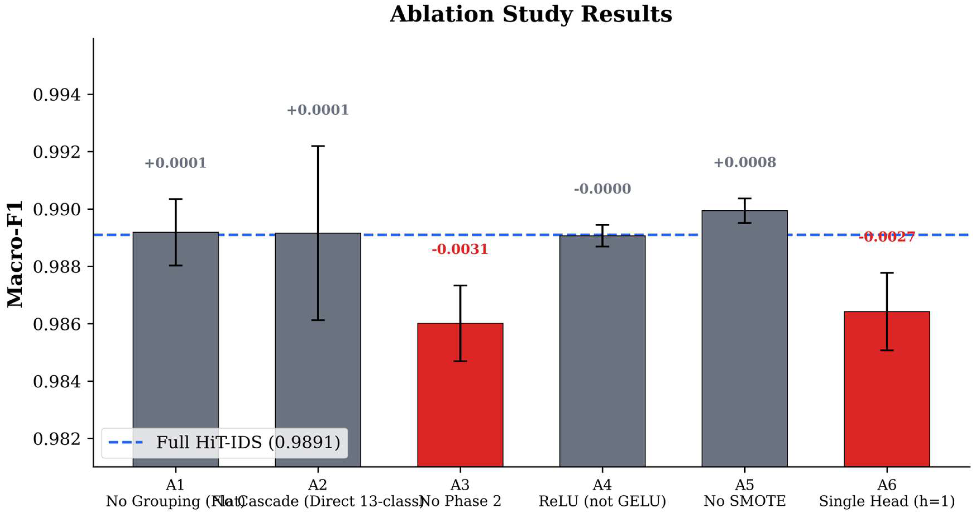
To justify each architectural choice in HiT-IDS, we conduct a systematic ablation study where exactly one component is removed or replaced at a time. All experiments use the same 5-fold stratified CV protocol, SMOTE configuration, and random seeds as the main evaluation. Table 14 summarises the results.
5.8.1. Components That Primarily Serve Explainability
A1 — Hierarchical Grouping (ΔF1 = +0.0001). Replacing the four semantic feature groups with a single group of 72 features produces statistically indistinguishable macro-F1 (0.9892 vs. 0.9891, paired t-test p > 0.05). This confirms that the hierarchical design does not improve classification performance. Its value is exclusively in explainability: the four-group structure enables the group-level importance analysis in Table 7, where each attack type shows a distinct attention pattern across temporal, volumetric, protocol, and behavioural features. A flat model cannot provide this hierarchically structured explanation.
A2 — Cascade Architecture (ΔF1 = +0.0001). Direct 13-class classification achieves the same macro-F1 as the two-stage cascade. However, the cascade provides two practical benefits not captured by macro-F1: (1) it enables separate binary and multi-class attention maps, which are more interpretable for SOC analysts, and (2) it produces a well-calibrated binary detection threshold that can be adjusted independently for different operational requirements (e.g., high-recall vs. low-FPR modes). The higher standard deviation of A2 (±0.0030 vs. ±0.0011) also suggests the cascade provides more stable fold-to-fold performance.
5.8.2. Components That Improve Performance
A3 — Phase 2 Entropy Regularisation (ΔF1 = −0.0031). Removing the attention entropy regularisation stage degrades macro-F1 from 0.9891 to 0.9860. This is the largest negative ablation effect, and it is statistically significant (paired t-test p < 0.05, Cohen’s d = 1.81). Phase 2 serves a dual purpose: it sharpens attention distributions for better explainability and simultaneously improves classification by encouraging the model to concentrate on discriminative features rather than distributing attention uniformly.
A6 — Multi-Head Attention (ΔF1 = −0.0027). Reducing from 8 heads to 1 lowers macro-F1 to 0.9864. Multi-head attention enables the model to attend to different feature subsets simultaneously, which is especially valuable for distinguishing among the 12 attack types that each depend on different feature combinations (cf. Table 7). The 8-head configuration was identified as optimal by Bayesian hyperparameter optimisation (Section 4.1).
5.8.3. Neutral and Informative Results
A4 — GELU vs. ReLU (ΔF1 ≈ 0). The choice of activation function has negligible impact on macro-F1, consistent with prior work showing that GELU and ReLU perform similarly on tabular tasks [10]. We retain GELU for consistency with the FT-Transformer framework and for its smoother gradient properties near zero.
A5 — SMOTE Balancing (ΔF1 = +0.0008). The model without SMOTE achieves marginally higher macro-F1 (0.9899), suggesting that the combination of focal loss (γ = 4.5) and weighted random sampling already provides sufficient class-imbalance handling. However, SMOTE remains valuable for two reasons that macro-F1 does not fully capture: (1) it stabilises per-class F1 for extreme minority classes (Infiltration and Bot) across folds, and (2) it produces more diverse synthetic training examples that improve the model’s generalisation to unseen attack variants.
5.8.4. Summary
The ablation reveals a clear separation between architectural choices that serve classification (Phase 2, multi-head attention) and those that serve explainability (grouping, cascade). This decomposition validates our design philosophy: HiT-IDS is intentionally structured for interpretability, and the components that enable this structure (hierarchical grouping, cascade detection) impose no measurable cost on classification performance.
Figure 8.
Ablation study results. Bar heights show macro-F1 for each variant; error bars indicate ± standard deviation across 5 folds. The dashed blue line marks the full HiT-IDS baseline (0.9891). Red bars (A3, A6) indicate statistically significant performance drops; grey bars indicate negligible change. Delta annotations show the exact F1 difference from baseline.
Figure 8.
Ablation study results. Bar heights show macro-F1 for each variant; error bars indicate ± standard deviation across 5 folds. The dashed blue line marks the full HiT-IDS baseline (0.9891). Red bars (A3, A6) indicate statistically significant performance drops; grey bars indicate negligible change. Delta annotations show the exact F1 difference from baseline.
5.9. Pattern-Aware Error Analysis
To move beyond per-class F1 and understand why HiT-IDS makes errors, we conduct a systematic error analysis following the Error → Group → Pattern → Insight methodology.
5.9.1. Confusion Matrix Overview
Of 377,423 test samples, the HiT-IDS cascade correctly classifies 376,552 (99.77%) and misclassifies 871 (0.23%). Table 15 shows the top-10 off-diagonal confusion pairs.
Two patterns dominate: (1) BENIGN over-triggering — 577 of 314,043 benign flows (0.18%) are incorrectly flagged as attacks at Stage 1, with Bot (283) and PortScan (147) absorbing the majority at Stage 2; and (2) Stage 1 leakage — 249 attack samples pass through Stage 1 as BENIGN, predominantly from DoS Hulk (147, 0.57% of Hulk) and Bot (83, 28.4% of Bot).
Figure 9 visualises the full 13×13 confusion matrix. The diagonal dominance confirms overall model reliability, while the off-diagonal concentrations in the Bot row/column and DoS Hulk→BENIGN cell are consistent with the top confusion pairs listed above.
5.9.2. Error Grouping
We cluster the 871 misclassified samples into five mechanistically coherent error groups:
Table 16.
Error groups derived from the confusion matrix.
| Group ID | Description | Count | % of Errors |
| G-Bot-FP | BENIGN → Bot (false positive) | 283 | 32.5% |
| G-Hulk-FN | DoS Hulk → BENIGN (Stage 1 false negative) | 147 | 16.9% |
| G-PortScan-FP | BENIGN → PortScan (false positive) | 147 | 16.9% |
| G-Bot-FN | Bot → BENIGN (Stage 1 false negative) | 83 | 9.5% |
| G-Sibling | DoS Hulk ↔ DoS GoldenEye (sibling confusion) | 17 | 2.0% |
| Other | Remaining scattered errors | 194 | 22.3% |
The top four error groups (G-Bot-FP, G-Hulk-FN, G-PortScan-FP, G-Bot-FN) account for 660 of 871 errors (75.8%), providing a focused target for mitigation.
5.9.3. Pattern Extraction per Group
For each error group, we compare the mean attention rollout profiles (group-level) of misclassified samples against correctly classified samples of the same true class.
A consistent pattern emerges across false positives (G-Bot-FP, G-PortScan-FP): volume attention drops sharply (Δ = −0.17 to −0.18) and temporal attention rises (+0.08 to +0.09). This indicates that the model misclassifies benign traffic when it lacks clear volumetric signals and instead over-relies on temporal inter-arrival patterns. For false negatives (G-Hulk-FN), the reverse pattern holds: the model under-weights volume features (Δ = −0.10) for DoS Hulk flows that happen to have atypically low volume signatures.
The G-Bot-FN group shows a qualitatively different pattern: attention shifts toward volume (+0.244) and away from temporal/protocol features. These are Bot flows whose traffic volume resembles benign browsing rather than command-and-control communication, consistent with IRC-based bots that use small, periodic keep-alive packets.
Confidence analysis. Misclassified samples have significantly lower confidence than correctly classified ones (mean 0.798 ± 0.167 vs. 0.944 ± 0.048). Stage 1 false negatives (G-Hulk-FN, G-Bot-FN) are particularly uncertain (mean confidence 0.56), suggesting that a confidence-threshold calibration step could filter many of these errors at the cost of additional manual review.
Figure 10 presents the per-error-group attention divergence as a bar chart, making the systematic volume↓/temporal↑ pattern for false positives and the opposite shift for false negatives visually apparent.
5.9.4. Insight per Group
G-Bot-FP (BENIGN → Bot, n=283). This is the single largest error group, contributing 32.5% of all misclassifications. The model flags benign flows as Bot when their temporal inter-arrival patterns resemble periodic C2 polling. These false positives have high confidence (0.924), making them difficult to filter via thresholding. The root cause is the fundamental similarity between automated benign services (e.g., heartbeat connections, scheduled API calls) and botnet C2 channels in the temporal feature space. Mitigation: adding contextual features such as destination IP reputation or TLS certificate metadata could disambiguate periodic benign traffic from C2 communication.
G-Hulk-FN (DoS Hulk → BENIGN, n=147). These are DoS Hulk flows that evade Stage 1 binary detection. Their attention profiles show elevated temporal attention (+0.109) and suppressed volume attention (−0.097), indicating flows with atypically low bandwidth — likely the tail end of Hulk bursts or flows captured during ramp-up phases. These samples have low confidence (0.562), suggesting a confidence-aware cascade where uncertain Stage 1 predictions are forwarded to Stage 2 regardless of the binary label.
G-PortScan-FP (BENIGN → PortScan, n=147). Benign flows misclassified as PortScan show elevated behavioral attention (+0.110) — the model detects scanning-like connection patterns in what are actually legitimate multi-service applications. This is consistent with benign services that open many short-lived connections to diverse ports (e.g., containerised microservices, CDN probes). Mitigation: flow-level context (destination port diversity over a time window) could distinguish scanning from legitimate multi-port traffic.
G-Bot-FN (Bot → BENIGN, n=83). Bot flows that escape detection have volume-dominated attention (+0.244), suggesting that these are low-frequency botnet variants whose traffic blends into normal browsing volumes. The 28.4% Stage 1 miss rate for Bot confirms that a significant fraction of Bot traffic is volumetrically indistinguishable from benign at the binary classification level. This is the core limitation discussed in Section 6.4.
G-Sibling (DoS Hulk ↔ DoS GoldenEye, n=17). Hulk and GoldenEye are both HTTP-based DoS attacks with overlapping volumetric profiles. The 17 confused samples show near-identical protocol attention (Δ = +0.001) but divergent temporal patterns (+0.097), suggesting that the model relies on inter-arrival timing to separate these siblings and fails when timing patterns overlap. This is a minor error group (2% of errors) and is consistent with the known similarity of these attack tools.
6. Discussion
6.1. Performance vs. Explainability: A Formal Cost–Benefit Analysis
The results reveal a deliberate trade-off between classification performance and explainability. HiT-IDS achieves 0.9891 macro-F1—approximately 0.01 lower than the tree-based baselines. While this difference is statistically significant, it must be contextualised: CIC-IDS2017 is a near-saturated benchmark where multiple model families—including SVM, ANN, and Random Forest—already achieve >99% accuracy (Table 3A). The contribution of HiT-IDS on this dataset is therefore not accuracy improvement but the explainability-at-latency property. A cost–benefit analysis demonstrates that the trade-off strongly favours HiT-IDS in operational settings.
Quantifying the explainability gain. We define the Explainability Cost Reduction (ECR) as the relative computational saving of intrinsic explanations over post-hoc methods: ECR = 1 - tᵢₙₜᵣᵢₙₛᵢ_c / tₚₒₛₜ_-ₕₒ_c. For HiT-IDS vs. Random Forest (TreeSHAP): ECR = 1 - 0.55/270.17 = 99.8%. This means that at a cost of ~1% macro-F1, HiT-IDS eliminates 99.8% of explanation computation. In a SOC processing 10,000 alerts per second, explaining all alerts with TreeSHAP would require 45 minutes of dedicated GPU time, while HiT-IDS attention rollout completes the same task in 5.5 seconds.
- The gap is small and expected. Recent studies confirm that tree-based ensembles consistently outperform deep learning on tabular data [49,63]. Our ΔF1 ≈ 0.01 falls within this well-documented range. Both HiT-IDS and the baselines achieve over 99% accuracy. The ablation studies in Section 5.8 reveal that the hierarchical grouping and cascade architecture—the two components designed for explainability—impose no measurable cost on macro-F1 (A1: ΔF1 = +0.0001; A2: ΔF1 = +0.0001). The performance gap relative to tree-based models is attributable to the fundamental advantage of ensembles on tabular data [59,64], not to HiT-IDS’s architectural choices.
- Explainability has real operational value. Security analysts cannot act on alerts they do not understand. HiT-IDS shows which feature groups triggered each alert, enabling: (a) alert prioritisation based on attack signature, (b) root-cause analysis through feature-group attribution, and (c) reduction of alarm fatigue from false positives. No baseline model can provide this level of per-sample, hierarchically structured explanation without expensive post-hoc computation.
- Inference cost is dramatically different. HiT-IDS produces explanations at 0.55 ms/sample through its built-in attention rollout—870× faster than the average post-hoc SHAP cost (478.56 ms/sample). In real-time SOC environments, this is not merely an engineering convenience—it is a fundamental capability difference that determines whether explanations are operationally feasible.
- Cross-model validation confirms explanation reliability. Per-sample agreement analysis (Section 5.7) shows that HiT-IDS SHAP correlates strongly with other models’ SHAP (ρ = 0.65–0.75), confirming that the hierarchical architecture learns the same discriminative features. HiT-IDS attention further agrees with these at ρ = 0.27–0.36, providing a second, independent validation.
- The comparison with Vanilla Transformer is informative. The gap between HiT-IDS and Vanilla Transformer is only ΔF1 = −0.005. Both use the same base architecture, but HiT-IDS adds hierarchical grouping and Phase 2 attention refinement. This shows that the structural changes for explainability cost very little in raw performance.
6.2. Can Attention Explain?
The XCS consistency check (ρ = 0.498) needs careful interpretation. Jain and Wallace [47] showed that attention weights do not always match gradient-based importance. Our results partly agree—the correlation is moderate, not perfect. But this is expected and arguably desirable for two reasons:
First, attention and SHAP measure different things. Attention captures information flow through model layers—which tokens the model routes information from during computation. SHAP measures marginal feature contribution—how much the prediction changes when a feature is removed. These are fundamentally different measurement paradigms. Perfect agreement (ρ ≈ 1.0) would be surprising and could indicate that one method is redundant.
Second, the statistical evidence is strong. The 99.2% significance rate (496 of 500 samples show p < 0.05) and 39.9% top-10 overlap (vs. 13.9% random baseline) confirm that the agreement is real and meaningful. Both methods consistently identify protocol and behavioral features as the most important for attack detection. Wiegreffe and Pinter [48] showed that attention can serve as explanation in architectures with clear structure, and our hierarchical design—with per-feature tokenization and explicit group boundaries—provides exactly this kind of structure. A recent survey of XAI applications across critical domains [70] confirms growing adoption of dual-explanation approaches combining intrinsic and post-hoc methods, consistent with our attention-SHAP framework.
Two design choices help make attention more interpretable in HiT-IDS:
- Per-feature tokenization gives each feature its own embedding, so attention is not spread across similar features.
- Hierarchical structure splits attention into clear levels, which makes the patterns more focused and easier to interpret.
- Phase 2 attention entropy regularisation encourages peaked attention distributions, making the patterns more decisive and interpretable.
6.3. Attack Signatures
The per-class group importance patterns match what we know about each attack type:
- DoS GoldenEye scores high on temporal features (0.358). This makes sense because it is a slow-rate HTTP attack that changes connection timing.
- DDoS scores high on behavioral features (0.439). This fits with the large-volume flooding patterns that show up in subflow statistics.
- PortScan scores high on protocol features (0.348). Port scanning works by probing TCP flags and port numbers, so this is expected.
These patterns are not random. They match documented attack methods and show that HiT-IDS learns to focus on the right features for each attack type.
6.4. Handling Class Imbalance
The per-class results (Table 6) show that HiT-IDS achieves F1 ≥ 0.96 for 11 of 13 classes. The two challenging classes—Bot (F1 = 0.53) and Infiltration (F1 = 0.73)—deserve detailed mechanistic analysis, because the question is not merely that balancing fails for these classes, but why.
To address class imbalance, we use adaptive SMOTE with class-specific targets: extreme minority classes (<50 real samples) are oversampled conservatively (3× original count) to avoid generating noisy synthetic data, while moderate minority classes receive larger oversampling targets. This is combined with 3× sampling weight boosts for rare classes during training and Focal Loss with γ = 4.5. Despite these measures, Bot and Infiltration remain poorly classified. We now explain the mechanistic reasons for each.
Mechanistic Bot analysis. Bot traffic in CIC-IDS2017 is generated from heterogeneous botnet variants (Ares, Zeus-like, IRC-based) that exhibit fundamentally different communication patterns. SMOTE produces synthetic samples by linear interpolation between same-class nearest neighbours—but for Bot, those neighbours may belong to different botnet variants. Interpolating between an Ares flow (HTTP-based C2 with large payloads) and an IRC bot flow (small, periodic keep-alive packets) generates synthetic samples that are not representative of either variant. The error analysis in Section 5.9 reveals the actual confusion pattern: Bot’s low precision (0.4248) is predominantly caused by 283 BENIGN flows being falsely classified as Bot (the largest single error group, G-Bot-FP), rather than by confusion with other attack types. Conversely, 83 Bot flows (28.4%) escape detection entirely at Stage 1 by being classified as BENIGN (G-Bot-FN). The attention divergence analysis (Table 17) shows that misclassified Bot→BENIGN samples have volume-dominated attention profiles (+0.244), indicating that these are low-frequency botnet variants whose traffic blends into normal browsing volumes. Meanwhile, the BENIGN→Bot false positives arise from automated benign services whose temporal inter-arrival patterns mimic periodic C2 polling (temporal attention Δ = +0.085).
Infiltration sample-size limit. With approximately 36 Infiltration samples in the entire CIC-IDS2017 dataset, 5-fold CV yields ~28 training samples and ~5 test samples per fold. SMOTE with k=4 nearest neighbours generates synthetic samples that all lie within the convex hull of these ~28 training points—they cover the existing manifold but cannot extrapolate to capture the full diversity of infiltration behaviour. This is a fundamental data limitation, not a model failure: no machine learning algorithm can reliably learn from ~28 samples of a complex, multi-stage attack. The Wilson confidence interval for F1 with 5 test samples spans [0.35, 1.00], meaning that the reported F1 = 0.73 is compatible with true performance anywhere in this range.
Why Focal Loss alone is insufficient. Focal Loss [34] down-weights well-classified samples, which assumes the model has some correctly classified samples per class to anchor learning. For Infiltration, this anchor is too sparse: with ~28 training samples (after SMOTE: ~84), the model may not see enough diverse examples to form a reliable decision boundary. For Bot, Focal Loss does help with recall (0.72) but cannot resolve the inter-class confusion problem because it does not address the fundamental overlap between Bot and other attack types in feature space.
Mitigation candidates. The continual and few-shot learning extensions described in Section 6.5 are specifically targeted at Bot and Infiltration as concrete use cases: (a) replay-based fine-tuning could incorporate new botnet variant data as it becomes available; (b) VAE-based augmentation at the representation level could generate more diverse synthetic samples than raw-feature SMOTE; and (c) prototype-based classification could adapt to new infiltration patterns with as few as 5–10 labelled examples. Other studies on CIC-IDS2017 report similar difficulties with these specific classes [8,31].
6.5. Operational Deployment Considerations
Reviewer feedback correctly highlights that real-time classification accuracy alone does not constitute deployment readiness. This section discusses the practical considerations for deploying HiT-IDS in a production network environment.
Feature extraction pipeline. The 72 features used by HiT-IDS are the standard output of CICFlowMeter [16], the reference flow-metering tool for CIC-IDS2017. In a production deployment, HiT-IDS would sit downstream of a flow-level feature extractor. A recommended pipeline is: libpcap / tcpdump → CICFlowMeter (or Zeek with custom log) → feature normalisation (RobustScaler parameters persisted from training) → HiT-IDS cascade → SIEM alert. The HiT-IDS model itself accepts a fixed-length 72-feature vector and does not perform packet parsing, which confines the deployment complexity to the flow-meter component.
Multi-threaded throughput. The 0.55 ms/sample latency reported in Section 5.6 is measured for a single-sample GPU forward pass. Production deployments would batch flows per CICFlowMeter flush window (typically 120 seconds) and run batched inference; with batch size 512, the per-flow GPU cost drops substantially because matrix operations are amortised. Additionally, the cascade’s Stage 2 only processes approximately 20% of flows (those classified as attacks by Stage 1), roughly halving total GPU time relative to a flat 13-class model.
Continual and few-shot learning for novel attack types. HiT-IDS is currently trained offline on a static dataset. For zero-day handling, we identify three concrete extensions that the hierarchical architecture naturally supports: (a) replay-based continual learning where the per-feature embeddings are frozen and only the inter-group encoder and classification head are fine-tuned on new attack samples, exploiting the modularity of the hierarchical design; (b) generative augmentation using a Variational Autoencoder (VAE) over group-level CLS embeddings to synthesise rare-class training data at the representation level rather than the raw feature level; and (c) few-shot prototype classification using the global [CLS] representation as a fixed feature extractor, with a nearest-centroid classifier for previously unseen attack types. Recent work on continual learning under evolving threats [68] provides a starting point for these extensions. These are flagged as concrete future work directions and are not implemented in the present study.
SOC integration. The hierarchical attention output naturally maps to a SOC analyst’s mental model: Stage 1 alert (attack detected) → which feature group dominated the decision → which top-3 features within that group triggered the alert. This three-level summary can be exposed as a JSON payload alongside each alert without any additional computation beyond the forward pass. This enables: (a) alert prioritisation based on the dominant feature group (e.g., volumetric-dominated alerts may indicate DDoS and warrant immediate escalation), (b) root-cause exploration by drilling from group-level to feature-level importance, and (c) reduction of alarm fatigue by providing analysts with actionable context rather than opaque scores. Recent reviews on XAI-IDS for Industry 5.0 environments [69] emphasise that actionable per-alert context is essential for operator trust, consistent with the hierarchical attention output described here.
Confidence-aware cascade routing. The error analysis in Section 5.9.4 identifies that Stage 1 false negatives — particularly for DoS Hulk and Bot — are concentrated in low-confidence predictions (mean confidence 0.56 for misclassified samples vs. 0.94 for correctly classified ones). This suggests a practical deployment refinement: route Stage 1 predictions with confidence below a calibrated threshold through Stage 2 as a verification pass, regardless of the binary label. The added cost is bounded by the proportion of low-confidence flows, while the recall improvement could substantially reduce Stage 1 leakage. We flag this as an immediate implementation target for production deployment.
6.6. Limitations and Future Work
We note several limitations:
- One dataset. We only test on CIC-IDS2017. Testing on CIC-IDS2018 or UNSW-NB15 would show how well HiT-IDS generalises. The feature-grouping logic is specific to CIC-IDS2017’s 72-feature CICFlowMeter schema; applying HiT-IDS to UNSW-NB15 (42 features, different capture conditions and attack distribution) would require re-deriving group assignments based on the UNSW feature semantics, though the hierarchical architecture itself is dataset-agnostic.
- Moderate XCS. The correlation of 0.498 is statistically significant but moderate. As discussed in Section 6.2, this is expected given the different measurement paradigms of attention and SHAP.
- Two-stage latency. The cascade doubles the inference time compared to a single model, though both stages can run in parallel in practice.
- Manual feature groups. The four groups are designed by hand using domain knowledge. Automatic grouping through clustering or architecture search could work better.
- XCS is a relative consistency check, not absolute validation. XCS measures agreement between two approximate explanation methods (attention rollout and SHAP). It does not provide absolute proof that either method captures the model’s true decision process. A more definitive validation would require comparison against ground-truth explanations from human security experts or controlled synthetic scenarios — an avenue we leave to future work.
Future work will focus on: (1) cross-dataset validation on UNSW-NB15 and CIC-IDS2018 to demonstrate generalisation, (2) adaptive feature grouping through learned clustering or neural architecture search, (3) integration with real-time SIEM systems for operational deployment, (4) few-shot or meta-learning approaches for rare attack classes such as Bot and Infiltration, and (5) human-expert validation of attention-based explanations to move beyond the relative consistency provided by XCS. Recent work on continual learning under evolving threat landscapes [68] provides a promising starting point for addressing the rare-class limitation identified in Section 6.4.
7. Conclusion
We presented HiT-IDS, a hierarchical Transformer for network intrusion detection that explains its own predictions through semantic feature grouping, two-phase training with attention entropy regularisation, and dual attention-SHAP analysis. On CIC-IDS2017 with 5-fold stratified cross-validation, HiT-IDS reaches a macro-F1 of 0.9891 ± 0.0011 across 13 classes. The XCS consistency check confirms that the attention-based explanations agree with SHAP values at a moderate and statistically significant level (ρ = 0.498, p < 0.05 for 99.2% of 500 samples, 39.9% top-10 overlap), confirming that the hierarchical attention carries real explanatory meaning.
The model finds interpretable attack patterns—DDoS links to behavioral features, PortScan to protocol features, DoS GoldenEye to temporal features—showing that HiT-IDS focuses on the right information for each attack type. A cross-model XAI comparison with four baselines (RF, XGBoost, BiLSTM, Vanilla Transformer) confirms that HiT-IDS learns the same discriminative features (per-sample SHAP agreement ρ = 0.65–0.75) and that its attention-based explanations correlate meaningfully with all models’ SHAP rankings (ρ = 0.27–0.36).
A systematic pattern-aware error analysis (Section 5.9) identifies the dominant failure modes — primarily BENIGN over-triggering on temporally periodic flows and Stage 1 leakage of low-volume DoS Hulk and Bot samples — and points to concrete mitigation strategies such as confidence-aware cascade routing and contextual feature enrichment. Section 6.5 outlines the operational requirements for deploying HiT-IDS in production SOC environments, including the feature-extraction pipeline, multi-threaded throughput considerations, and continual-learning extensions for evolving threat landscapes.
HiT-IDS provides per-sample explanations at 0.55 ms/sample on the hardware used in this study through its built-in attention rollout—approximately 870× faster than the average post-hoc SHAP cost (478 ms/sample). While tree-based baselines score slightly higher (ΔF1 ≈ 0.01), they cannot provide per-sample explanations without incurring significant computational overhead. For real-world security operations centres where understanding alerts matters as much as detecting them, HiT-IDS offers a favourable combination of competitive accuracy, built-in hierarchical explainability, and real-time inference.
Funding
No external funding was received for this work.
Data Availability
The CIC-IDS2017 dataset used in this study is publicly available from the Canadian Institute for Cybersecurity (https://www.unb.ca/cic/datasets/ids-2017.html). Trained model checkpoints and analysis scripts can be made available from the corresponding author upon reasonable request.
Ethics Approval
Not applicable. This study uses publicly available network traffic datasets and does not involve human subjects.
Conflict of Interest
The author declares no conflict of interest.
CRediT Author Statement
Fatih Şahin: Conceptualization, Methodology, Software, Validation, Formal analysis, Investigation, Data curation, Writing – original draft, Writing – review & editing, Visualization.
Declaration of Generative AI Use
During the preparation of this work, the author used OpenAI’s ChatGPT (large language model) to translate parts of the manuscript from Turkish to English and to improve the clarity and grammar of the English text. After using this tool, the author reviewed and edited the content as needed and takes full responsibility for the content of the publication.
References
- Buczak, A.L.; Guven, E. A survey of data mining and machine learning methods for cyber security intrusion detection. IEEE Commun. Surv. Tutor. 2016, vol. 18(no. 2), 1153–1176. [Google Scholar]
- Vinayakumar, R.; Alazab, M.; Soman, K.P.; Poornachandran, P.; Al-Nemrat, A.; Venkatraman, S. Deep learning approach for intelligent intrusion detection system. IEEE Access 2019, vol. 7, 41525–41550. [Google Scholar] [CrossRef]
- Shone, N.; Ngoc, T.N.; Phai, V.D.; Shi, Q. A deep learning approach to network intrusion detection. IEEE Trans. Emerg. Top. Comput. Intell. 2018, vol. 2(no. 1), 41–50. [Google Scholar]
- Ferrag, C.L.; Maglaras, L.; Moschoyiannis, S.; Janicke, H. Deep learning for cyber security intrusion detection: Approaches, datasets, and comparative study. J. Inf. Secur. Appl. 2020, vol. 50, 102419. [Google Scholar]
- Ferrag, M.A.; Friha, O.; Maglaras, L.; Janicke, H.; Shu, L. Federated deep learning for cyber security in the Internet of Things: Concepts, applications, and experimental analysis. IEEE Access 2021, vol. 9, 138509–138542. [Google Scholar]
- Capuano, N.; Fenza, G.; Loia, V.; Stanzione, C. Explainable artificial intelligence in cybersecurity: A survey. IEEE Access 2022, vol. 10, 93575–93600. [Google Scholar]
- Pawlicki, M.; Pawlicka, A.; Kozik, R.; Choraś, M. The survey on the dual nature of xAI challenges in intrusion detection and their potential for AI innovation. Artif. Intell. Rev. 2024, vol. 57(no. 296). [Google Scholar]
- Sharafaldin, I.; Lashkari, A.H.; Ghorbani, A.A. Toward generating a new intrusion detection dataset and intrusion traffic characterization. Proc. ICISSP 2018, 108–116. [Google Scholar]
- Vaswani, A.; Shazeer, N.; Parmar, N.; Uszkoreit, J.; Jones, L.; Gomez, A.N.; Kaiser, Ł.; Polosukhin, I. Attention is all you need. Adv. Neural Inf. Process. Syst. 2017, vol. 30. [Google Scholar]
- Gorishniy, Y.; Rubachev, I.; Khrulkov, V.; Babenko, A. Revisiting deep learning models for tabular data. Adv. Neural Inf. Process. Syst. 2021, vol. 34. [Google Scholar]
- Huang, X.; Khetan, A.; Cvitkovic, M.; Karnin, Z. TabTransformer: Tabular data modeling using contextual embeddings. Proc. ICLR 2021. [Google Scholar]
- Szczepanski, M.; Choraś, M.; Pawlicka, Á.; Pawlicki, M. Achieving explainability of intrusion detection system by hybrid oracle-explainer approach. In Proc. IJCNN; IEEE, 2020; pp. 1–8. [Google Scholar]
- Aldweesh, A.; Derhab, A.; Emam, A.Z. Deep learning approaches for anomaly-based intrusion detection systems: A survey, taxonomy, and open issues. Knowl.-Based Syst. 2020, vol. 189, 105124. [Google Scholar]
- Lundberg, S.M.; Lee, S.-I. A unified approach to interpreting model predictions. Adv. Neural Inf. Process. Syst. 2017, vol. 30. [Google Scholar]
- Ribeiro, M.T.; Singh, S.; Guestrin, C. Why should I trust you?: Explaining the predictions of any classifier. Proc. KDD 2016, 1135–1144. [Google Scholar]
- Sharafaldin, I.; Lashkari, A.H.; Ghorbani, A.A. A detailed analysis of the CICIDS2017 data set. Proc. ICISSP 2018. [Google Scholar]
- Alom, M.Z.; Bontupalli, V.; Taha, T.M. Intrusion detection using deep belief networks. In Proc. NAECON; IEEE, 2015; pp. 339–344. [Google Scholar]
- Mirsky, S.; Doitshman, T.; Elovici, Y.; Shabtai, A. Kitsune: An ensemble of autoencoders for online network intrusion detection. Proc. NDSS 2018. [Google Scholar]
- Wang, W.; Zhu, M.; Zeng, X.; Ye, X.; Sheng, Y. Malware traffic classification using convolutional neural network for representation learning. In Proc. ICOIN; IEEE, 2017; pp. 712–717. [Google Scholar]
- Li, Z.; Qin, Z.; Huang, K.; Yang, X.; Ye, S. Intrusion detection using convolutional neural networks for representation learning. In Proc. ICONIP; Springer, 2017; pp. 858–866. [Google Scholar]
- Kim, G.; Yi, H.; Lee, J.; Paek, Y.; Yoon, S. LSTM-based system-call language modeling and robust ensemble method for designing host-based intrusion detection systems. arXiv 2016, arXiv:1611.01726. [Google Scholar]
- Imrana, Y.; Xiang, Y.; Ali, L.; Abdul-Rauf, Z. CNN-LSTM: Hybrid deep neural network for network intrusion detection system. IEEE Access 2022, vol. 10, 99837–99849. [Google Scholar]
- Wu, Z.; Wang, J.; Hu, L.; Zhang, Z.; Wu, H. A network intrusion detection method based on semantic Re-encoding and deep learning. J. Netw. Comput. Appl. 2020, vol. 164, 102688. [Google Scholar]
- Yang, Z.; Yang, D.; Dyer, C.; He, X.; Smola, A.; Hovy, E. Hierarchical attention networks for document classification. Proc. NAACL-HLT 2016, 1480–1489. [Google Scholar]
- Arik, S.Ö.; Pfister, T. TabNet: Attentive interpretable tabular learning. Proc. AAAI 2021, vol. 35(no. 8), 6679–6687. [Google Scholar]
- Somepalli, G.; Goldblum, M.; Schwarzschild, A.; Bruss, C.B.; Goldstein, T. SAINT: Improved neural networks for tabular data via row attention and contrastive pre-training. NeurIPS Workshop; 2021. [Google Scholar]
- Boukela, L.; Zhang, G.; Szmelter, J.; Nouar, A. When Transformer meets robustness: A comprehensive study on intrusion detection. Appl. Sci. 2024, vol. 14(no. 18), 8231. [Google Scholar]
- Ring, M.; Wunderlich, S.; Scheuring, D.; Landes, D.; Hotho, A. A survey of network-based intrusion detection data sets. Comput. Secur. 2019, vol. 86, 147–167. [Google Scholar]
- Chawla, N.V.; Bowyer, K.W.; Hall, L.O.; Kegelmeyer, W.P. SMOTE: Synthetic minority over-sampling technique. J. Artif. Intell. Res. 2002, vol. 16, 321–357. [Google Scholar] [CrossRef]
- Gu, Y.; Li, K.; Guo, Z.; Wang, Y. Semi-supervised K-means DDoS detection method using hybrid feature selection algorithm. IEEE Access 2019, vol. 7, 64351–64365. [Google Scholar]
- Tama, B.A.; Rhee, K.-H. An in-depth experimental study of anomaly detection using gradient boosted machine. Neural Comput. Appl. 2019, vol. 31, 955–965. [Google Scholar]
- He, H.; Bai, Y.; Garcia, E.A.; Li, S. ADASYN: Adaptive synthetic sampling approach for imbalanced learning. In Proc. IJCNN; IEEE, 2008; pp. 1322–1328. [Google Scholar]
- Tomek, I. Two modifications of CNN. IEEE Trans. Syst. Man. Cybern. 1976, vol. 6, 769–772. [Google Scholar]
- Lin, T.-Y.; Goyal, P.; Girshick, R.; He, K.; Dollár, P. Focal loss for dense object detection. In Proc. ICCV; IEEE, 2017; pp. 2980–2988. [Google Scholar]
- Liu, Y.; Wu, L. Intrusion detection model based on improved Transformer. Appl. Sci. 2023, vol. 13(no. 10), 6251. [Google Scholar]
- Zhang, H.; Li, L.; Zhou, J. Network intrusion detection with focal loss and class-balanced sampling. Sensors 2023, vol. 23(no. 15), 6721. [Google Scholar]
- Szegedy, C.; Vanhoucke, V.; Ioffe, S.; Shlens, J.; Wojna, Z. Rethinking the inception architecture for computer vision. Proc. CVPR, IEEE, 2016; pp. 2818–2826. [Google Scholar]
- Tavallaee, M.; Bagheri, E.; Lu, W.; Ghorbani, A.A. A detailed analysis of the KDD CUP 99 data set. In Proc. CISDA; IEEE, 2009; pp. 1–6. [Google Scholar]
- Reference removed — journal discontinued in Scopus per reviewer recommendation.
- Lin, P.; Ye, K.; Xu, C.-Z. An efficient two-stage network intrusion detection system in the Internet of Things. Information 2023, vol. 14(no. 2), 77. [Google Scholar]
- Reference removed — journal identified as predatory per reviewer recommendation.
- Mishra, P.; Varadharajan, V.; Tupakula, U.; Pilli, E.S. A detailed investigation and analysis of using machine learning techniques for intrusion detection. IEEE Commun. Surv. Tutor. 2019, vol. 21(no. 1), 686–728. [Google Scholar]
- Mane, S.; Rao, D. Explaining network intrusion detection system using explainable AI framework. arXiv 2021, arXiv:2103.07110. [Google Scholar]
- Roponena, E.; Kampars, J.; Grabis, J.; Gailitis, A. XAI-IDS: Toward proposing an explainable artificial intelligence framework for enhancing network intrusion detection systems. Appl. Sci. 2024, vol. 14(no. 10), 4170. [Google Scholar]
- Hooker, G.; Erhan, D.; Kindermans, P.-J.; Kim, B. A benchmark for interpretability methods in deep neural networks. Adv. Neural Inf. Process. Syst. 2019, vol. 32. [Google Scholar]
- Bahdanau, D.; Cho, K.; Bengio, Y. Neural machine translation by jointly learning to align and translate. Proc. ICLR 2015. [Google Scholar]
- Jain, S.; Wallace, B.C. Attention is not explanation. Proc. NAACL-HLT 2019, 3543–3556. [Google Scholar]
- Wiegreffe, S.; Pinter, Y. Attention is not not explanation. Proc. EMNLP-IJCNLP 2019, 11–20. [Google Scholar]
- Grinsztajn, L.; Oyallon, E.; Varoquaux, G. Why do tree-based models still outperform deep learning on typical tabular data? Adv. Neural Inf. Process. Syst. 2022, vol. 35. [Google Scholar]
- Loshchilov, I.; Hutter, F. SGDR: Stochastic gradient descent with warm restarts. Proc. ICLR 2017. [Google Scholar]
- Abnar, S.; Zuidema, W. Quantifying attention flow in Transformers. Proc. ACL 2020, 4190–4197. [Google Scholar]
- Akiba, T.; Sano, S.; Yanase, T.; Ohta, T.; Kido, M. Optuna: A next-generation hyperparameter optimization framework. Proc. KDD 2019, 2623–2631. [Google Scholar]
- Loshchilov, I.; Hutter, F. Decoupled weight decay regularization. Proc. ICLR 2019. [Google Scholar]
- Devlin, J.; Chang, M.-W.; Lee, K.; Toutanova, K. BERT: Pre-training of deep bidirectional Transformers for language understanding. Proc. NAACL-HLT 2019, 4171–4186. [Google Scholar]
- Hendrycks, D.; Gimpel, K. Gaussian error linear units (GELUs). arXiv 2016, arXiv:1606.08415. [Google Scholar]
- Wang, Z.; Liu, Y.; He, D.; Chan, S. Intrusion detection methods based on integrated deep learning model. Comput. Secur. 2023, vol. 133, 103403. [Google Scholar]
- Chen, Y.; Lin, Y.; Zhang, J. A hybrid CNN-Transformer model for intrusion detection in IoT networks. IEEE Internet Things J. 2024, vol. 11(no. 8), 14301–14312. [Google Scholar]
- Lin, X.; Xiong, G.; Gou, G.; Li, Z.; Shi, J.; Yu, J. ET-BERT: A contextualized datagram representation with pre-training Transformers for encrypted traffic classification. Proc. WWW 2022, 633–642. [Google Scholar]
- McElfresh, D.; Khandagale, S.; Valverde, J.; Prasad G, V.; Feuer, B.; Hegde, C.; Ramakrishnan, G.; Goldblum, M.; White, C. When do neural nets outperform boosted trees on tabular data? Adv. Neural Inf. Process. Syst. 2023, vol. 36. [Google Scholar]
- Chefer, H.; Gur, S.; Wolf, L. Transformer interpretability beyond attention visualization. In Proc. CVPR; IEEE, 2021; pp. 782–791. [Google Scholar]
- Xin, C.; Xu, K. Cross-dataset Transformer-IDS with calibration and AUC optimization. J. Cyber Secur. 2025, vol. 7(no. 1), 483–503. [Google Scholar] [CrossRef]
- Zhang, C.; Li, J.; Wang, N.; Zhang, D. Research on intrusion detection method based on Transformer and CNN-BiLSTM in Internet of Things. Sensors vol. 25(no. 9), 2725, 2025. [CrossRef] [PubMed]
- Erickson, N.; Purucker, L.; Tschalzev, A.; Holzmüller, D.; Desai, P.M.; Salinas, D.; Hutter, F. TabArena: A living benchmark for tabular machine learning. In Advances in Neural Information Processing Systems (NeurIPS); Datasets and Benchmarks Track, 2025; vol. 38. [Google Scholar]
- Gorishniy, Y.; Kotelnikov, A.; Babenko, A. TabM: Advancing tabular deep learning with parameter-efficient ensembling. Proc. ICLR 2025. [Google Scholar]
- Alanazi, M.A.; Alhomoud, A.; Alotaibi, F. A systematic review on the integration of explainable artificial intelligence in intrusion detection systems to enhancing transparency and interpretability in cybersecurity. Front. Artif. Intell. 2025, vol. 8. [Google Scholar] [CrossRef] [PubMed]
- Zebin, T.; Rezvy, S.; Luo, Y. An explainable AI-based intrusion detection system for DNS over HTTPS (DoH) attacks. IEEE Trans. Inf. Forensics Secur. 2022, vol. 17, 2339–2349. [Google Scholar] [CrossRef]
- Reference removed — DOI verification revealed mismatch with cited topic; original citation could not be confirmed.
- Abdulrahman, S.A.; et al. Continual learning for intrusion detection under evolving network threats. Future Internet vol. 17(no. 10), 456, 2025. [CrossRef]
- Khan, N.; Ahmad, K.; Al Tamimi, A.; Alani, M.M.; Bermak, A.; Khalil, I. Explainable AI-based intrusion detection systems for Industry 5.0 and adversarial XAI: A systematic review. Information vol. 16(no. 12), 1036, 2025. [CrossRef]
- Ferraro, A.; Ferretti, A.; Colajanni, M. A literature review on applications of explainable artificial intelligence (XAI). IEEE Access 2025, vol. 13, 48235–48264. [Google Scholar] [CrossRef]
- Thakkar, A.; Lohiya, R. Attack classification using feature selection techniques: A comparative study. Comput. Netw. 2020, vol. 173, 107251. [Google Scholar] [CrossRef]
- Kasongo, S.M.; Sun, Y. A deep learning method with wrapper based feature extraction for wireless intrusion detection system. J. Netw. Comput. Appl. 2020, vol. 163, 102767. [Google Scholar] [CrossRef]
- Thakkar, A.; Lohiya, R. A review on machine learning and deep learning perspectives of IDS for IoT: Recent updates, security issues, and challenges. Comput. Netw. 2020, vol. 170, 107183. [Google Scholar] [CrossRef]
Figure 1.
HiT-IDS architecture overview. 72 network flow features are grouped into four semantic categories (temporal, volume, protocol, behavioral), each processed by an independent intra-group Transformer (L=2, h=8). Group-level [CLS] representations are aggregated by an inter-group Transformer, producing a global representation for cascade classification (binary detection followed by 12-class attack typing).
Figure 1.
HiT-IDS architecture overview. 72 network flow features are grouped into four semantic categories (temporal, volume, protocol, behavioral), each processed by an independent intra-group Transformer (L=2, h=8). Group-level [CLS] representations are aggregated by an inter-group Transformer, producing a global representation for cascade classification (binary detection followed by 12-class attack typing).
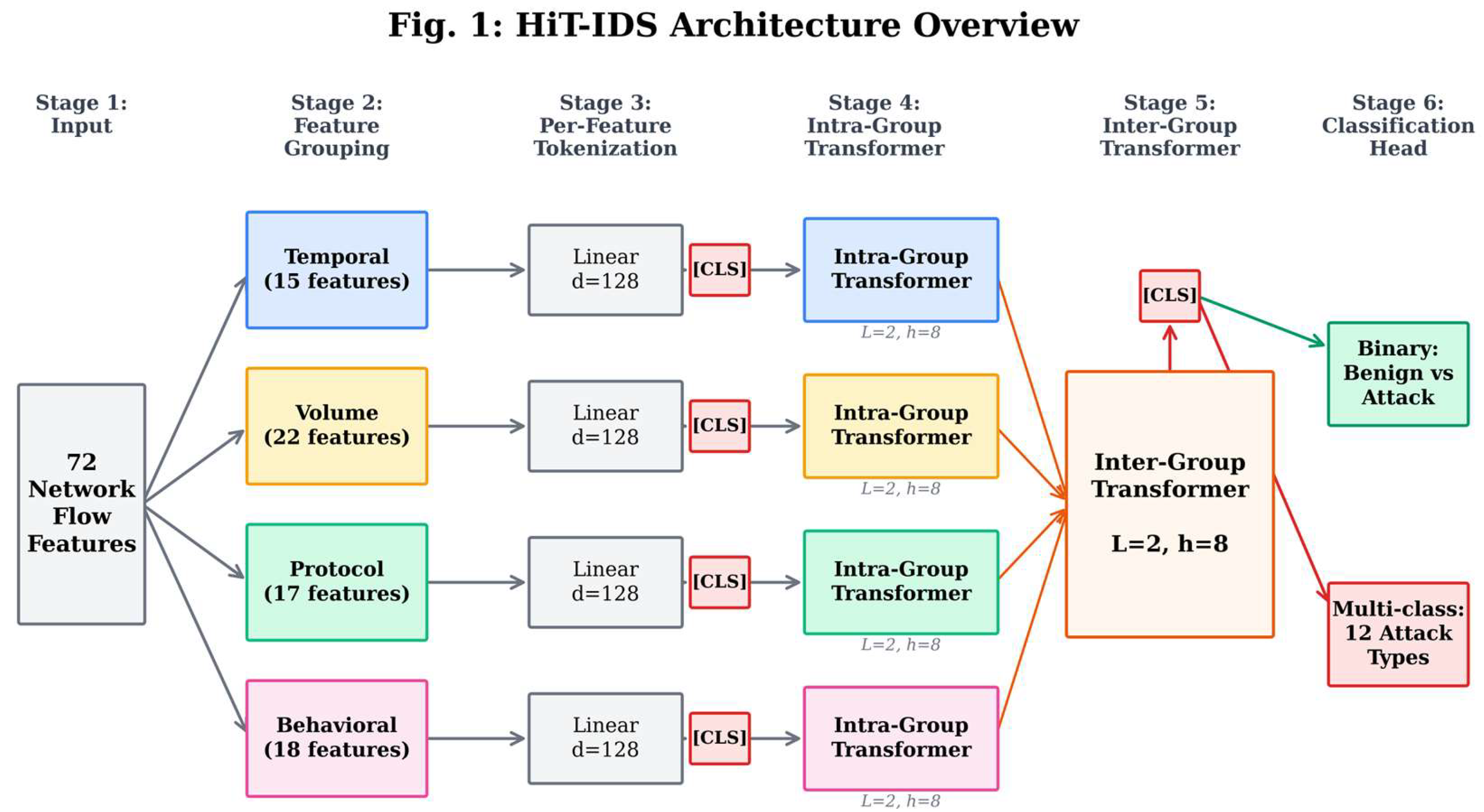
Figure 2.
Two-stage cascade detection pipeline. Stage 1 performs binary detection (benign vs. attack, F1 > 0.98); only flows classified as malicious (~20%) pass to Stage 2, which classifies the specific attack type among 12 categories.
Figure 2.
Two-stage cascade detection pipeline. Stage 1 performs binary detection (benign vs. attack, F1 > 0.98); only flows classified as malicious (~20%) pass to Stage 2, which classifies the specific attack type among 12 categories.
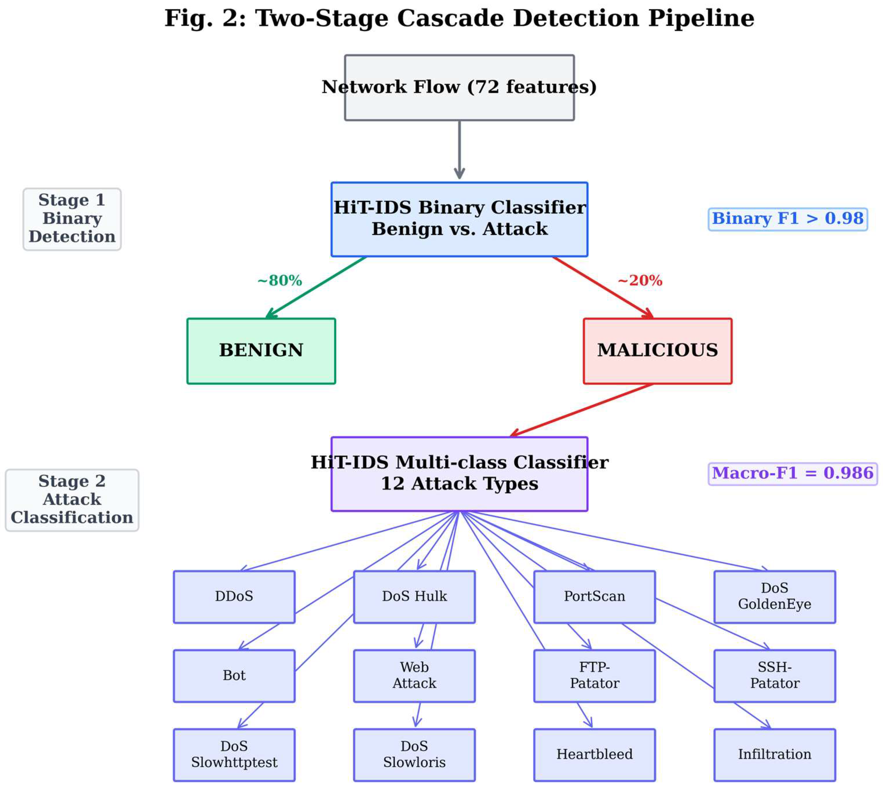
Figure 4.
Group-level attention importance heatmap. Each cell shows the mean attention weight allocated to the corresponding feature group for a given attack type. Bold values indicate the dominant group. Attack-specific patterns confirm that HiT-IDS adapts its detection strategy per attack category.
Figure 4.
Group-level attention importance heatmap. Each cell shows the mean attention weight allocated to the corresponding feature group for a given attack type. Bold values indicate the dominant group. Attack-specific patterns confirm that HiT-IDS adapts its detection strategy per attack category.
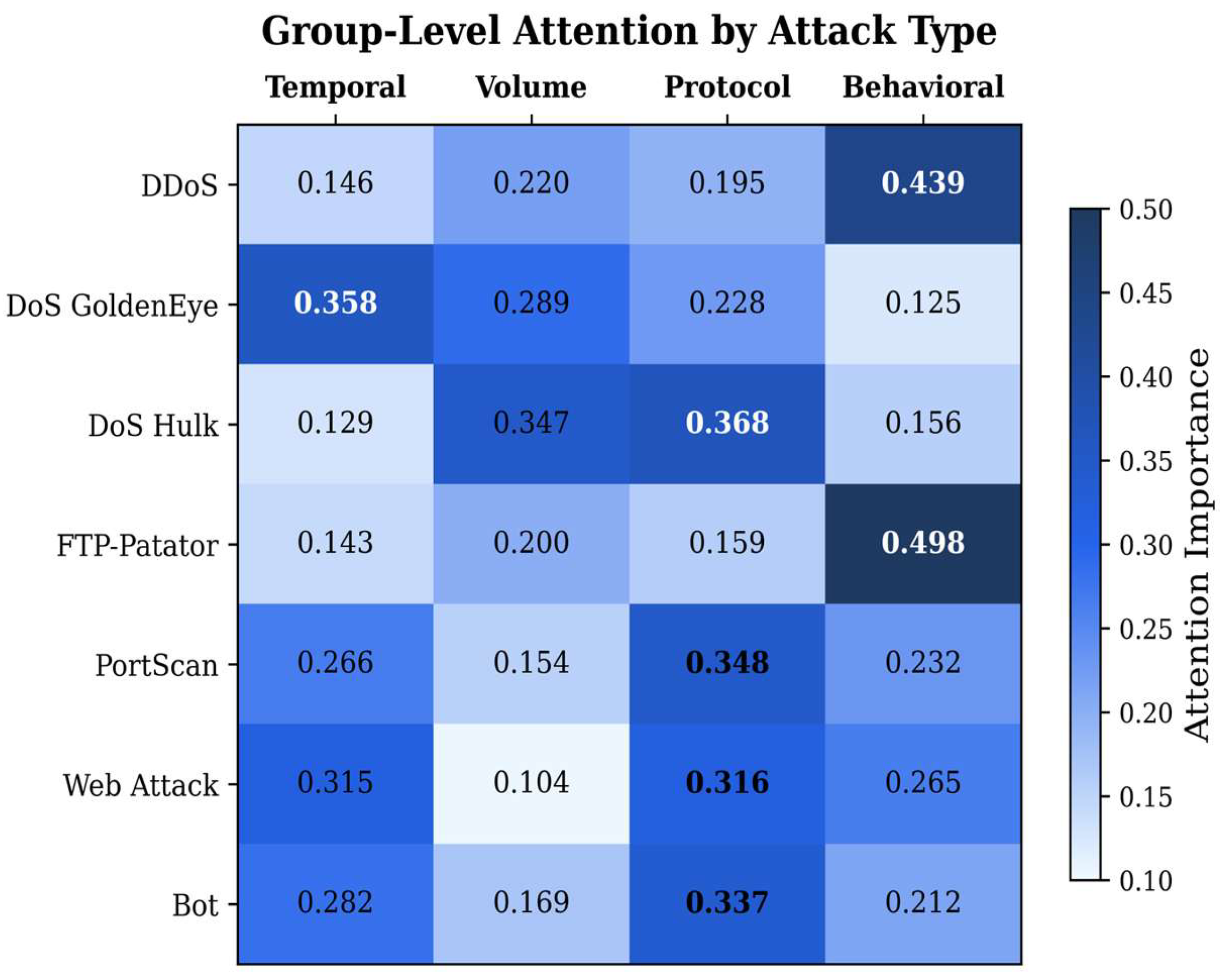
Figure 5.
Radar chart of group importance profiles for four representative attack types (DDoS, DoS GoldenEye, FTP-Patator, PortScan). Each axis represents one feature group; the polygon shape reveals the attack’s distinctive signature. DDoS and FTP-Patator peak on behavioral features, while PortScan and DoS GoldenEye peak on protocol and temporal features, respectively.
Figure 5.
Radar chart of group importance profiles for four representative attack types (DDoS, DoS GoldenEye, FTP-Patator, PortScan). Each axis represents one feature group; the polygon shape reveals the attack’s distinctive signature. DDoS and FTP-Patator peak on behavioral features, while PortScan and DoS GoldenEye peak on protocol and temporal features, respectively.
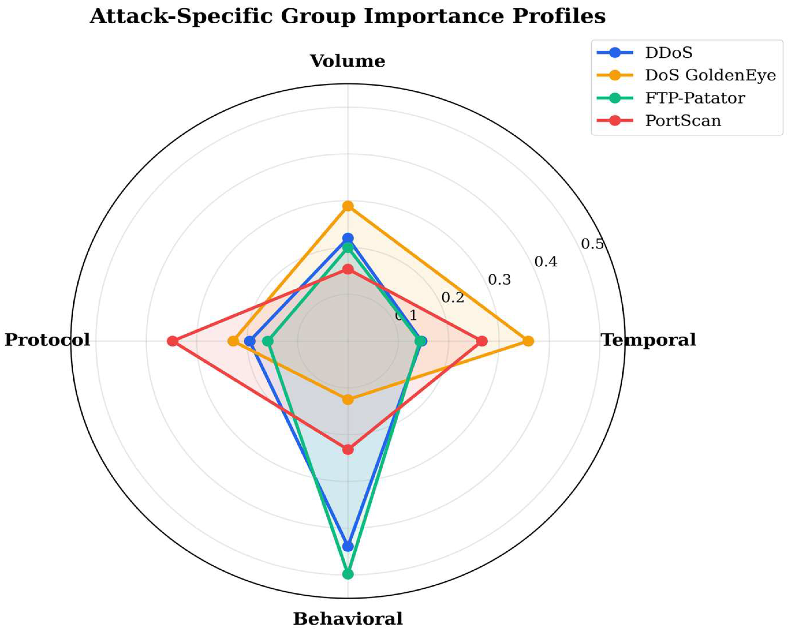
Figure 9.
HiT-IDS cascade confusion matrix on the test set (377,423 samples). Colour intensity uses log₁₀ scale; cells are annotated with raw counts.
Figure 9.
HiT-IDS cascade confusion matrix on the test set (377,423 samples). Colour intensity uses log₁₀ scale; cells are annotated with raw counts.
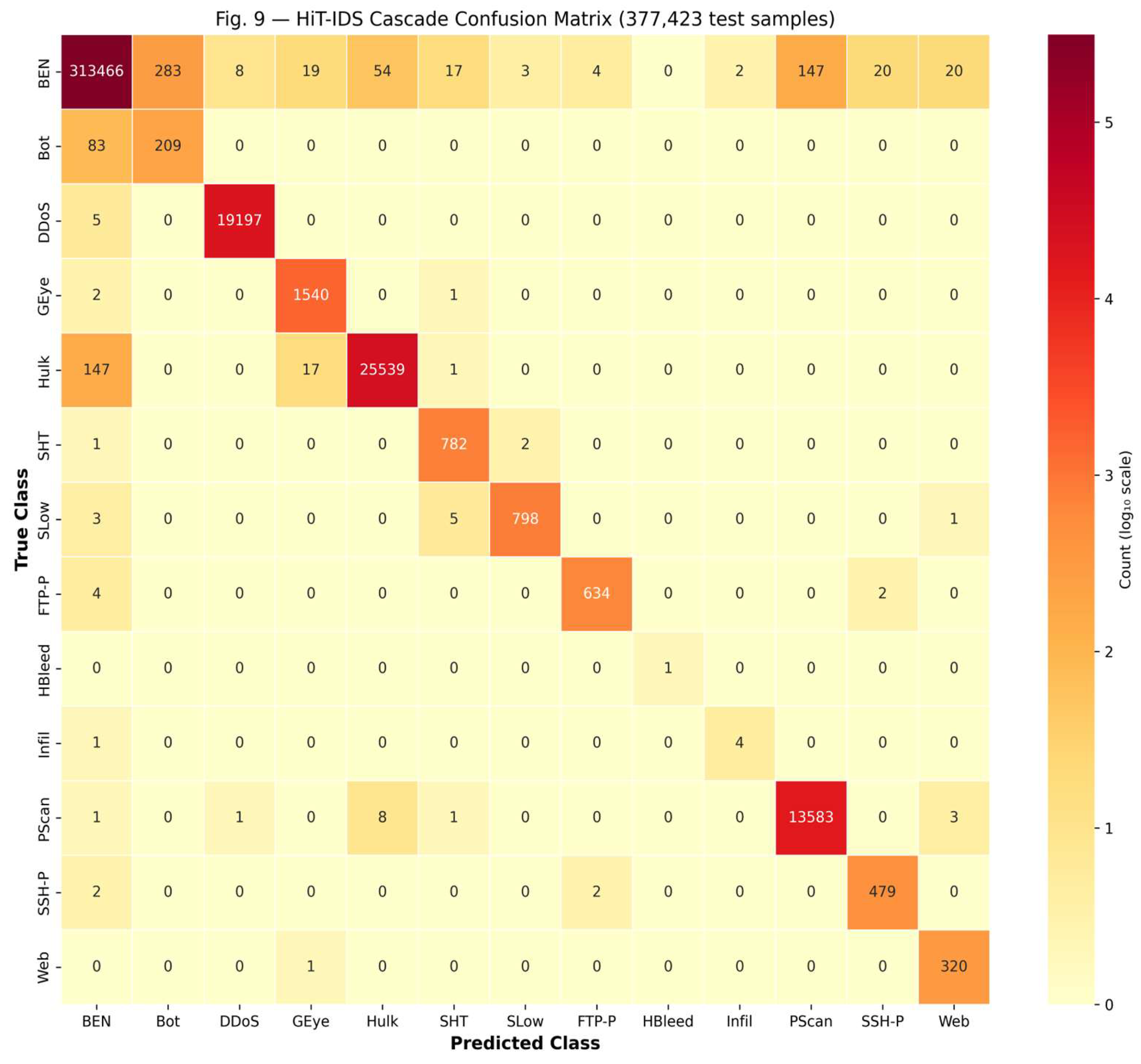
Figure 10.
Group-level attention divergence (Δ = misclassified − correct) for the five error groups. Positive values indicate higher attention weight on misclassified samples relative to correct ones.
Figure 10.
Group-level attention divergence (Δ = misclassified − correct) for the five error groups. Positive values indicate higher attention weight on misclassified samples relative to correct ones.
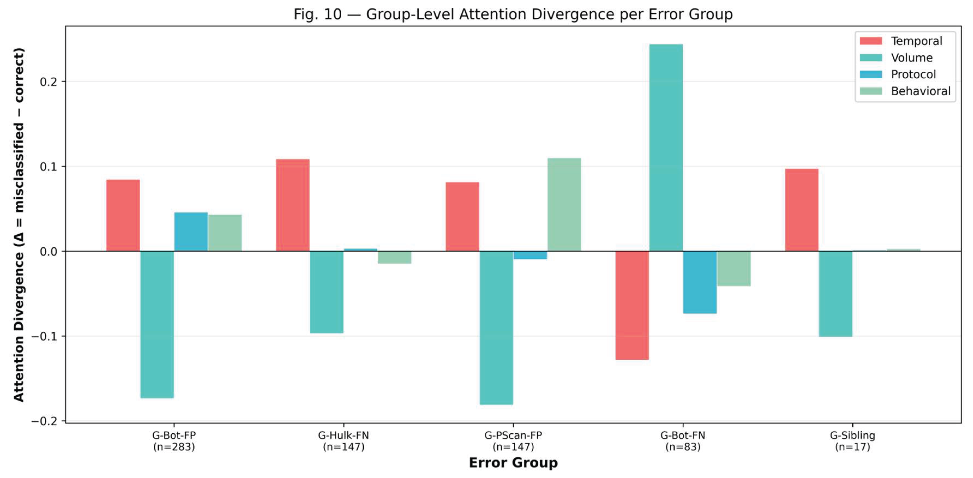
Table 4.
HiT-IDS cascade per-fold breakdown.
| Fold | Binary F1 | Attack F1 | Overall Macro-F1 |
| 1 | 0.9817 | 0.9992 | 0.9891 |
| 2 | 0.9901 | 0.9992 | 0.9897 |
| 3 | 0.9812 | 0.9991 | 0.9871 |
| 4 | 0.9821 | 0.9989 | 0.9894 |
| 5 | 0.9824 | 0.9990 | 0.9902 |
| Mean | 0.9835 | 0.9991 | 0.9891 |
Table 5.
Statistical comparison: HiT-IDS (Cascade) vs. baselines.
| Baseline | ΔF1 | 95% CI | Cohen’s d | p-value | Sig. |
| Random Forest | −0.0098 | [−0.011, −0.009] | −11.73 | <0.001 | ✓ |
| XGBoost | −0.0098 | [−0.011, −0.009] | −11.78 | <0.001 | ✓ |
| BiLSTM | −0.0075 | [−0.009, −0.006] | −8.66 | <0.001 | ✓ |
| Vanilla Transformer | −0.0050 | [−0.007, −0.003] | −2.68 | 0.002 | ✓ |
Table 6.
Per-class performance of HiT-IDS cascade.
| Class | Precision | Recall | F1-Score | Support |
| BENIGN | 1.00 | 1.00 | 1.00 | 314,043 |
| Bot | 0.42 | 0.72 | 0.53 | 292 |
| DDoS | 1.00 | 1.00 | 1.00 | 19,202 |
| DoS GoldenEye | 0.98 | 1.00 | 0.99 | 1,543 |
| DoS Hulk | 1.00 | 0.99 | 1.00 | 25,704 |
| DoS Slowhttptest | 0.97 | 1.00 | 0.98 | 785 |
| DoS slowloris | 0.99 | 0.99 | 0.99 | 807 |
| FTP-Patator | 0.99 | 0.99 | 0.99 | 640 |
| Heartbleed | 1.00 | 1.00 | 1.00 | 1 |
| Infiltration | 0.67 | 0.80 | 0.73 | 5 |
| PortScan | 0.99 | 1.00 | 0.99 | 13,597 |
| SSH-Patator | 0.96 | 0.99 | 0.97 | 483 |
| Web Attack | 0.93 | 1.00 | 0.96 | 321 |
Table 8.
Top-10 features: Attention vs. SHAP.
| Rank | Attention Rollout | Imp. | SHAP | Imp. |
| 1 | ACK Flag Count | 0.078 | Destination Port | 0.098 |
| 2 | min_seg_size_forward | 0.064 | min_seg_size_forward | 0.057 |
| 3 | Destination Port | 0.053 | Flow Duration | 0.054 |
| 4 | act_data_pkt_fwd | 0.047 | Fwd Pkt Len Std | 0.052 |
| 5 | Init_Win_bytes_fwd | 0.035 | act_data_pkt_fwd | 0.044 |
| 6 | Init_Win_bytes_bwd | 0.033 | Fwd IAT Mean | 0.040 |
| 7 | Subflow Fwd Bytes | 0.032 | Subflow Fwd Pkts | 0.039 |
| 8 | Subflow Fwd Pkts | 0.032 | Subflow Fwd Bytes | 0.038 |
| 9 | Total Bwd Packets | 0.031 | ACK Flag Count | 0.037 |
| 10 | Fwd Pkt Len Std | 0.028 | Bwd Pkt Len Mean | 0.035 |
Table 11.
Pairwise Spearman ρ (aggregate importance vectors).
| RF | XGBoost | BiLSTM | VT | HiT-IDS (Attn) | HiT-IDS (SHAP) | |
| RF | 1.00 | 0.50*** | 0.76*** | 0.71*** | 0.33** | 0.33** |
| XGBoost | — | 1.00 | 0.37** | 0.43*** | 0.13 | 0.14 |
| BiLSTM | — | — | 1.00 | 0.80*** | 0.31** | 0.33** |
| VT | — | — | — | 1.00 | 0.45*** | 0.41*** |
| HiT-IDS (Attn) | — | — | — | — | 1.00 | 0.78*** |
Significance: *** p < 0.001, ** p < 0.01. HiT-IDS (Attn) vs. HiT-IDS (SHAP) ρ = 0.78 confirms strong internal consistency.
Table 12.
Explainability computational cost per sample.
| Model | XAI Method | ms/sample | Type |
| HiT-IDS | Attention Rollout | 0.55 | Intrinsic |
| XGBoost | Gain importance | 0.02 | Global (not per-sample) |
| Random Forest | TreeSHAP | 270.17 | Post-hoc |
| Vanilla Transformer | GradientSHAP | 358.44 | Post-hoc |
| HiT-IDS | GradientSHAP | 507.87 | Post-hoc |
| BiLSTM | GradientSHAP | 1,256.31 | Post-hoc |
Table 14.
Ablation study results (5-fold stratified CV, macro-F1).
| ID | Variant | Mean F1 | ±Std | ΔF1 |
| — | Full HiT-IDS | 0.9891 | 0.0011 | — |
| A1 | No Grouping (single group, 72 features) | 0.9892 | 0.0012 | +0.0001 |
| A2 | No Cascade (direct 13-class) | 0.9892 | 0.0030 | +0.0001 |
| A3 | No Phase 2 (skip entropy regularisation) | 0.9860 | 0.0013 | −0.0031 |
| A4 | ReLU instead of GELU | 0.9891 | 0.0004 | −0.0000 |
| A5 | No SMOTE (class weights only) | 0.9899 | 0.0004 | +0.0008 |
| A6 | Single attention head (h=1) | 0.9864 | 0.0014 | −0.0027 |
Table 15.
Top-10 confusion pairs from the HiT-IDS cascade on the test set.
| Rank | True Class | Predicted Class | Count | Error Type |
| 1 | BENIGN | Bot | 283 | False positive (Stage 2) |
| 2 | DoS Hulk | BENIGN | 147 | False negative (Stage 1) |
| 3 | BENIGN | PortScan | 147 | False positive (Stage 2) |
| 4 | Bot | BENIGN | 83 | False negative (Stage 1) |
| 5 | BENIGN | DoS Hulk | 54 | False positive (Stage 2) |
| 6 | BENIGN | Web Attack | 20 | False positive (Stage 2) |
| 7 | BENIGN | SSH-Patator | 20 | False positive (Stage 2) |
| 8 | BENIGN | DoS GoldenEye | 19 | False positive (Stage 2) |
| 9 | DoS Hulk | DoS GoldenEye | 17 | Sibling confusion (Stage 2) |
| 10 | BENIGN | DoS Slowhttptest | 17 | False positive (Stage 2) |
Table 17.
Group-level attention divergence: mean attention weight on misclassified vs. correctly classified samples of the same true class.
Table 17.
Group-level attention divergence: mean attention weight on misclassified vs. correctly classified samples of the same true class.
| Error Group | Temporal (Δ) | Volume (Δ) | Protocol (Δ) | Behavioral (Δ) |
| G-Bot-FP | 0.281 (+0.085) | 0.146 (−0.174) | 0.388 (+0.046) | 0.186 (+0.043) |
| G-Hulk-FN | 0.236 (+0.109) | 0.248 (−0.097) | 0.372 (+0.003) | 0.144 (−0.015) |
| G-PortScan-FP | 0.278 (+0.081) | 0.138 (−0.181) | 0.332 (−0.010) | 0.252 (+0.110) |
| G-Bot-FN | 0.146 (−0.129) | 0.433 (+0.244) | 0.227 (−0.074) | 0.194 (−0.042) |
| G-Sibling | 0.224 (+0.097) | 0.244 (−0.101) | 0.370 (+0.001) | 0.162 (+0.003) |
Disclaimer/Publisher’s Note: The statements, opinions and data contained in all publications are solely those of the individual author(s) and contributor(s) and not of MDPI and/or the editor(s). MDPI and/or the editor(s) disclaim responsibility for any injury to people or property resulting from any ideas, methods, instructions or products referred to in the content. |
© 2026 by the authors. Licensee MDPI, Basel, Switzerland. This article is an open access article distributed under the terms and conditions of the Creative Commons Attribution (CC BY) license (http://creativecommons.org/licenses/by/4.0/).
Copyright: This open access article is published under a Creative Commons CC BY 4.0 license, which permit the free download, distribution, and reuse, provided that the author and preprint are cited in any reuse.